Stochastic Averaging Principle for Dynamical Systems with Fractional Brownian Motion

Abstract

Stochastic averaging for a class of stochastic differential equations (SDEs) with fractional Brownian motion, of the Hurst parameter $H$ in the interval $(\frac{1}{2},1)$, is investigated. An averaged SDE for the original SDE is proposed, and their solutions are quantitatively compared. It is shown that the solution of the averaged SDE converges to that of the original SDE in the sense of mean square and also in probability. It is further demonstrated that a similar averaging principle holds for SDEs under stochastic integral of pathwise backward and forward types. Two examples are presented and numerical simulations are carried out to illustrate the averaging principle.

Key words. correlated noise; Averaging principle; Stochastic differential equations;
Stochastic calculus; Fractional Brownian motion.

2000 Mathematics Subject Classification. Primary: 34F05, 37H10, 60H10, 93E03.

1 Introduction

Stochastic averaging is often used to approximate dynamical systems under random fluctuations. This analytic technique has been developed in the case of the Gaussian random fluctuations, for example, by Stratonovich [1, 2] and then by Khasminskii [3, 4]. It has been found to be effective for understanding stochastic differential equations arising in many fields [5, 6, 7]. Zhu and his co-workers further studied this stochastic averaging method for nonlinear systems under Poisson noise [8, 9, 10], and two of the present authors derived an averaging principle for stochastic differential equations with Lévy noise [11]. In all of these mentioned works, the fluctuations or noises are uncorrelated, i.e., white noises.
 However, random fluctuations with long-range dependence, or correlated noises, are abundant. They may be modeled by fractional Brownian motion (fBm) with $\frac{1}{2}<H<1$ (where $H$ is the Hurst index). The fractional Brownian motion was introduced by Kolmogorov [12]. Then, in 1968, Mandelbrot and Van Ness [13] presented the structure of the fractional Brownian motion. Due to the importance of long-range dependence of the fBm, the stochastic differential equations with fBm have been used as the model of the practical problems in various fields, such as hydrology, queueing theory and mathematical finance (Chakravarti and Sebastian, [14]; Hu and Øksendal, [15]; Leland, Taqqu, Willinger, and Wilson et al, [16]; Scheffer, [17]). So fractional Brownian motion has also been suggested as a replacement of standard Brownian motion in several stochastic models ([18, 19, 20]).

 Given the abundance of correlated fluctuations, it is crucial to understand the behaviors of the stochastic differential equations with fBm [21, 22, 23, 24]. Unfortunately, the fractional Brownian motion is neither a semi-martingale nor a Markov process, so the powerful tools for the stochastic integral theories are not applicable when studying fBm. Therefore, much of the recent research on SDEs with fBm is by numerical simulations. Other techniques for such SDEs would be desirable. This motivates us to investigate stochastic averaging techniques for differential equations driven by fractional Brownian motion.

In the present paper, we study a stochastic averaging technique for a class of SDEs with fBm. We present an averaging principle, and prove that the original stochastic differential equation can be approximated by an averaged stochastic differential equation in the sense of mean square convergence and convergence in probability, when a scaling parameter tends to zero. In addition, the similar conclusion holds for a SDE, where the stochastic differential or stochastic integral is of forward and backward types.

 The organization of the paper is as follows. Section 2 recalls the definition of fractional Brownian motion and highlight the differences with the usual Brownian motion roughly, and then briefly reviews the symmetric, forward and backward stochastic integrals with respect to fBm. Section 3 is devoted to prove a stochastic averaging principle for stochastic differential equations with fBm. Section 4 presents two examples to illustrate the stochastic averaging principle.

2 Fractional Brownian motion and stochastic integration

Since stochastic differential equations are interpreted via stochastic integrals, it is necessary to specify the integration with respect to fBm. For background on this issue, see [25, 26, 27, 28, 29]. For instance, using the notions of fractional integral and derivative, it is appropriate to introduce a pathwise stochastic integral with respect to fBm [30, 31, 32].

In this preliminary section, we briefly recall the definition of fBm and the integration with respect to it, for $H\in(\frac{1}{2},1)$.

2.1 Fractional Brownian motion

Let $(\Omega,\mathscr{F},P)$ be a complete probability space. The definition of the fractional Brownian motion is as follows[13].

Definition 1.

The fractional Brownian motion ($B^{H}(t)$) with Hurst index $H$ is a centered self-similar Gaussian process $B^{H}={B^{H}(t),t\in\mathbb{R_{+}}}$, on $(\Omega,\mathscr{F},P)$ with the properties :
(1) $B^{H}(0)=0$ ;
(2) $\mathbb{E}{B^{H}(t)}=0,t\in\mathbb{R_{+}}$ ;
(3) $\mathbb{E}{B^{H}(t)B^{H}(s)}=\frac{1}{2}(|t|^{2H}+|s|^{2H}-|t-s|^{2H}),t,s\in\mathbb{R_{+}}$.

For $H=\frac{1}{2}$, this is the usual Brownian motion.

We also recall the following features of the fractional Brownian motion:

(a) Self-similarity : For every constant $a>0$ and every $T>0$, the following relation about distribution (or law) holds

$$Law\quad(B^{H}(at):t\in[0,T])=Law\quad(a^{H}B^{H}(t):t\in[0,T]).$$

The above formula means that the two processes $B^{H}(at)$ and $a^{H}B^{H}(t)$ have the same finite-dimensional distribution functions, i.e., for every choice of $t_{0},\ldots,t_{n}\in\mathbb{R_{+}}$,

$$P(B^{H}(at_{0})\leq x_{0},\ldots,B^{H}(at_{n})\leq x_{n})=P(a^{H}B^{H}(t_{0})\leq x_{0},\ldots,a^{H}B^{H}(t_{n})\leq x_{n}),$$

for every $x_{0},\ldots,x_{n}\in\mathbb{R}$.

(b) Stationary increments : The increment of this process in $(s,t)$ has a normal distribution with zero mean, and the following variance

$$\mathbb{E}{(B^{H}(t)-B^{H}(s))^{2}}=|t-s|^{2H}.$$

Hence, for every integer $k\geq 1$,

$$\mathbb{E}{(B^{H}(t)-B^{H}(s))^{2k}}=\frac{2k!}{k!2^{k}}|t-s|^{2Hk}.$$

In other words, the parameter $H$ controls the regularity of the trajectories. For $H=\frac{1}{2}$, the increments of the process in disjoint intervals are independent, while for $H\neq\frac{1}{2}$, the increments are dependent.

(c) Long-range dependence : The auto-covariance function $\rho_{H}(n),n\in N$ of the fBm is

$$\quad\quad\quad\rho_{H}(n):=Cov(B^{H}(k)-B^{H}(k-1),B^{H}(k+n)-B^{H}(k+n-1))$$

$$=\frac{1}{2}[(n+1)^{2H}+(n-1)^{2H}-2n^{2H}]$$

$$\approx H(2H-1)n^{2H-2},$$

and $\rho_{H}(n)\longrightarrow 0$, as n tends to infinity.
 If $H>\frac{1}{2},\;\rho_{H}(n)>0$, for $n$ large enough, and $\sum_{n=1}^{\infty}\rho_{H}(n)=\infty$. In this case, we say that the fractional Brownian motion has long-range dependence. So the fBm can be used to describe cluster phenomena, occuring in geophysics, hydrology and economics.
 Based on the definition of the fractional Brownian motion, it is clear that the standard Brownian motion is a specific fractional Brownian motion with index $H=1/2$.
 The relationship between the usual Brownian motion and fractional Brownian motion is as follows:
(R1) The similarities : They are both Gaussian process; they do not have differentiable sample paths and both have statistical self-similarity; besides they are almost everywhere Hölder continuous.
(R2) The differences : Fractional Brownian motion is neither a semi-martingale nor a Markov process (for $H\neq\frac{1}{2}$), but the usual Brownian motion is a semi-martingale and a Markov process; fractional Brownian motion has no independent increments, while the usual Brownian motion has.

2.2 Stochastic integration with respect to fractional Brownian motion

For the convenience of readers, we recall some stochastic integration with respect to the fractional Brownian motion [33, 34, 35].
Let $\varphi:\mathbb{R}_{+}\times\mathbb{R}_{+}\longrightarrow\mathbb{R}_{+}$ be given by

$$\varphi(t,s)=H(2H-1)|t-s|^{2H-2},t,s\in\mathbb{R}_{+},$$

where $\frac{1}{2}<H<1$, and let $f:\mathbb{R}_{+}\longrightarrow\mathbb{R}_{+}$ be Borel measurable. Define

$$L_{\varphi}^{2}=\{f:|f|_{\varphi}^{2}=\int_{\mathbb{R}}\int_{\mathbb{R}}f(t)f(s)\varphi(t,s)dsdt<\infty\}.$$

The Hilbert space $L_{\varphi}^{2}$ is naturally associated with the Gaussian process $(B^{H}(t),t\geq 0)$.
Let $\mathcal{S}$ be the set of smooth and cylindrical random variables of the form

$$F=f(B^{H}(\psi_{1}),B^{H}(\psi_{2}),\ldots,B^{H}(\psi_{n})),$$

where $n\geq 1$, $f\in\mathcal{C}_{b}^{\infty}(\mathbb{R}^{n})$ (i.e., $f$ and all its partial derivatives are bounded), and $\psi_{i}\in\mathcal{H}$, $\mathcal{H}$ is a Hilbert space [29].
 Introduce the Malliavin $\varphi-derivative$ of $F$

$$D_{t}^{\varphi}F=\int_{\mathbb{R}}\varphi(t,\nu)D^{H}Fd\nu,$$

where

$$D^{H}F=\sum_{i=1}^{n}\frac{\partial f}{\partial x_{i}}(B^{H}(\psi_{1}),\ldots,B^{H}(\psi_{n}))\psi_{i}.$$

In this paper, we consider the pathwise stochastic integrals for fBm. The definition of the symmetric stochastic integral for the fBm case is in [33].

Definition 2.

Let $u(t)$ $(t\in[0,T])$ be a stochastic process with integrable trajectories. The symmetric integral of $u(t)$ with respect to $B^{H}(t)$ is defined as

$$\lim_{\epsilon\rightarrow 0}\frac{1}{2\epsilon}\int_{0}^{T}u(s)[B^{H}(s+\epsilon)-B^{H}(s-\epsilon)]ds,$$

provided that the limit exists in probability, and is denoted by $\int_{0}^{T}u(s)d^{\circ}B^{H}(s)$.

Remark 1.

Let $L(0,T)$ be the family of processes on $[0,T]$, such that $u(t)\in L(0,T)$ if $\mathbb{E}|u(t)|_{\varphi}^{2}<\infty$. Assume that $u(t)$ $(t\in[0,T])$ is a stochastic process in $L(0,T)$ and satisfies

$$\int_{0}^{T}\int_{0}^{T}|D_{s}^{H}u(t)||t-s|^{2H-2}dsdt<\infty.$$

Then the symmetric integral exists and the following relation holds:

$$\int_{0}^{T}u(t)d^{\circ}B^{H}(t)=\int_{0}^{T}u(t)\diamond dB^{H}(t)+\int_{0}^{T}D_{s}^{\varphi}u(s)ds,$$ (1)

where $\diamond$ denotes the Wick product, $H\in(\frac{1}{2},1)$.

Remark 2.

The definition of the forward and backward integrals with respect to fBm is as follows:
Let $u(t)$ $(t\in[0,T])$ be a process with integrable trajectories. The forward integral of $u(t)$ with respect to $B^{H}(t)$ is defined as

$$\lim_{\epsilon\rightarrow 0}\frac{1}{\epsilon}\int_{0}^{T}u(s)[\frac{B^{H}(s+\epsilon)-B^{H}(s)}{\epsilon}]ds,$$

provided that the limit exists in probability, and is denoted by $\int_{0}^{T}u(s)d^{-}B^{H}(s)$.

The backward integral is defined as

$$\lim_{\epsilon\rightarrow 0}\frac{1}{\epsilon}\int_{0}^{T}u(s)[\frac{B^{H}(s-\epsilon)-B^{H}(s)}{\epsilon}]ds,$$

provided that the limit exists in probability, and is denoted by $\int_{0}^{T}u(s)d^{+}B^{H}(s)$.

Remark 3.

According to [33], under the assumptions in Remark $1$, the symmetric, backward and forward integrals coincide in the following sense

$$\int_{0}^{T}u(t)d^{-}B^{H}(t)=\int_{0}^{T}u(t)\diamond dB^{H}(t)+\int_{0}^{T}D_{s}^{\varphi}u(s)ds,$$ (2)

$$\int_{0}^{T}u(t)d^{+}B^{H}(t)=\int_{0}^{T}u(t)\diamond dB^{H}(t)+\int_{0}^{T}D_{s}^{\varphi}u(s)ds.$$ (3)

3 An averaging principle for SDEs with fBm

3.1 Some Lemmas

In order to present a stochastic averaging principle, we need two lemmas.

Lemma 1.

Let $B^{H}(t)$ be a fractional Brownian motion with $\frac{1}{2}<H<1$, and $Z(s)$ be a stochastic process in $L[0,T]$ . For every $T<\infty$ , there exists a constant $C(H,T)=HT^{2H-1}$ such that

$$\mathbb{E}[(\int_{0}^{T}|Z(s)|\diamond dB^{H}(s))^{2}]\leq C(H,T)\mathbb{E}[\int_{0}^{T}|Z(s)|^{2}ds]+CT^{2}.$$ (4)

Proof.  According to [34] ( $Theorem$ $2.1$ ),

$$\mathbb{E}{\int_{0}^{T}(D_{s}^{\varphi}|Z(s)|)^{2}ds}<\infty,$$

and

$$\mathbb{E}{(\int_{0}^{T}|Z(s)|\diamond dB^{H}(s))^{2}}=\mathbb{E}{[||Z||_{\varphi}^{2}+\int_{0}^{T}D_{s}^{\varphi}|Z(s)|ds)^{2}]}.$$

Thus,

$$\mathbb{E}{(\int_{0}^{T}|Z(s)|\diamond dB^{H}(s))^{2}}=\mathbb{E}{[\int_{0}^{T}\int_{0}^{T}Z(t)Z(s)\varphi(t,s)dsdt}+\mathbb{E}{(\int_{0}^{T}D_{s}^{\varphi}Z(s)ds)^{2}}$$

$$\quad\quad\quad\quad\quad\quad\quad\quad\quad\quad\quad\triangleq A+B,$$

where

$$\quad\quad\quad\quad A=\mathbb{E}{\int_{0}^{T}\int_{0}^{T}|Z(t)||Z(s)|\varphi(t,s)dsdt},$$

$$B=\mathbb{E}{(\int_{0}^{T}D_{s}^{\varphi}|Z(s)|ds)^{2}}.$$

We further have

$$A\leq H(2H-1)\mathbb{E}{\int_{0}^{T}\int_{0}^{T}|Z(s)|^{2}|t-s|^{2H-2}dsdt}$$

$$\leq H(2H-1)\mathbb{E}{\int_{0}^{T}|Z(s)|^{2}\frac{1}{2H-1}T^{2H-1}ds}$$

$$\leq HT^{2H-1}\mathbb{E}{\int_{0}^{T}|Z(s)|^{2}}ds$$

$$\leq C(H,T)\mathbb{E}{\int_{0}^{T}|Z(s)|^{2}ds}.$$

By the Cauchy-Schwarz inequality for $B$ , we get :

$$B\leq T^{2}\mathbb{E}{\int_{0}^{T}|D_{s}^{\varphi}|Z(s)||^{2}ds}\leq CT^{2}.$$

Then we can finally deduce that

$$\mathbb{E}[(\int_{0}^{T}|Z(s)|\diamond dB^{H}(s))^{2}]\leq C(H,T)\mathbb{E}{\int_{0}^{T}|Z(s)|^{2}ds}+CT^{2}.$$

This finishes the proof of this Lemma.

Lemma 2 can be obtained according to Definition 4 and Lemma 1.

Lemma 2.

Suppose that Z(s) is a stochastic process in $L[0,T]$, and $B^{H}(t)(H>\frac{1}{2})$ is a fractional Brownian motion. For any $0<T<\infty$, there exists a constant $C(H,T)$, such that the following inequality holds

$$\mathbb{E}[(\int_{0}^{T}|Z(s)|d^{\circ}B^{H}(s))^{2}]\leq 2C(H,T)\mathbb{E}[\int_{0}^{T}|Z(s)|^{2}ds]+4CT^{2},$$ (5)

where $C(H,T)=HT^{2H-1}$ .

Proof.  Using Eq.(1) and the Cauchy-Schwarz inequality, we can get

$$\mathbb{E}[(\int_{0}^{T}|Z(s)|d^{\circ}B^{H}(s))^{2}]=\mathbb{E}[(\int_{0}^{T}|Z(s)|\diamond dB^{H}(s)+\int_{0}^{T}D_{s}^{\varphi}|Z(s)|ds)^{2}]$$

$$\leq\mathbb{E}[2(\int_{0}^{T}|Z(s)|\diamond B^{H}(s))^{2}+2(\int_{0}^{T}D_{s}^{\varphi}|Z(s)|ds)^{2}]$$

$$\leq 2\mathbb{E}[(\int_{0}^{T}|Z(s)|\diamond B^{H}(s))^{2}]+2\mathbb{E}[\int_{0}^{T}D_{s}^{\varphi}|Z(s)|ds^{2}],$$

Due to Eq.(4) and

$$\mathbb{E}{(\int_{0}^{T}D_{s}^{\varphi}|Z(s)|ds)^{2}}\leq CT^{2},$$

we obtain

$$\mathbb{E}[(\int_{0}^{T}|Z(s)|d^{\circ}B^{H}(s))^{2}]\leq 2C(H,T)\mathbb{E}{\int_{0}^{T}|Z(s)|^{2}ds}+2CT^{2}+2CT^{2},$$

namely

$$\mathbb{E}[(\int_{0}^{T}|Z(s)|d^{\circ}B^{H}(s))^{2}]\leq 2C(H,T)\mathbb{E}[\int_{0}^{T}|Z(s)|^{2}ds]+4CT^{2}.$$

the proof is completed.

3.2 Stochastic differential equations driven by fractional Brownian motion

In this section, we concern the symmetric integral of stochastic differential equations with respect to fBm. Solutions of the stochastic differential equation driven by fractional Browinan motion have been studied intensively by using the pathwise approach [36, 37].
Consider the equation on $\mathbb{R}^{d}$

$$X(t)=X(0)+\int_{0}^{t}b(s,X(s))ds+\int_{0}^{t}\sigma(s,X(s))d^{\circ}B^{H}(s),$$ (6)

where $X(0)$ is a given $d$-dimensional random variable, $b(s,X(s)):[0,T]\times\mathbb{R}^{d}\longrightarrow\mathbb{R}^{d}$ is a measurable vector function, $\sigma(s,X(s))isad\times m$ matrix with each element $\sigma_{j,i}(s,X(s)):[0,T]\times\mathbb{R}^{d}\longrightarrow\mathbb{R}^{d}$ a measurable vector function, and the processes $B^{H}(t)$, represents $d$-dimensional fractional Brownian motions with Hurst parameter $H$ defined in a complete probability space $(\Omega,\mathcal{F},\mathbb{P})$. Denote by $\sigma=(\sigma_{j,i})_{i,j=1}^{d,m}$ the matrix of ”diffusion” and $b=(b_{i})_{i=1}^{d}$ the ”drift” vector, $|\sigma|:=(\sum_{i,j}|\sigma_{j,i}|^{2})^{\frac{1}{2}}$ , $|b|:=(\sum_{i}(b_{i})^{2})^{\frac{1}{2}}$ .

Let us consider the following assumptions on the coefficients :

$\sigma(t,x)$ is differentiable in $x$ , and satisfies : there exists $M>0$ , $0<\gamma$ , $k\leq 1$ , and for any $N>0$, $M_{N}>0$,
(i) $\sigma$ is Lipschitz continous in $x$ ,$\forall$ $x$, $y\in\mathbb{R}^{d}$ , $t\in[0,T]$ :

$$|\sigma(t,x)-\sigma(t,y)|\leq M|x-y|,$$

(ii) $x$ -derivative of $\sigma$ is local Hölder continous in $x$ , $\forall$ $|x|,|y|\leq N,t\in[0,T]$

$$|\sigma_{x}(t,x)-\sigma_{x}(t,y)|\leq M_{N}|x-y|^{k},$$

(iii) $\sigma$ is Hölder continous in times, for all $x\in\mathbb{R}^{d},t,s\in[0,T]$ :

$$|\sigma(t,x)-\sigma(s,x)|+|\sigma_{x_{i}}(t,x)-\sigma_{x_{i}}(s,x)|\leq M|t-s|^{\gamma}.$$

for each $i=0,\ldots,d$.

The function $b=b(t,x)$ satisfies the following conditions:
(iv) for all $N\geq 0$ , there exist $L_{N}>0$ , for all $|x|,|y|\leq N,t\in[0,T]$ , such that

$$|b(t,x)-b(t,y)|\leq L_{N}|x-y|,$$

(v) there exists the function $b_{0}\in L_{p}(0,T;\mathbb{R}^{d})$ $(p\geq 2)$ , and $L>0$ , for any $(t,x)\in[0,T]\times\mathbb{R}$ such that

$$|b(t,x)|\leq L|x|+b_{0}(t).$$

On the basis of $Theorem$ $3.1.4$ and $Remark$ $3.1.5$ in [35], there exists the unique solution $(X_{t},t\in[0,T])$ of the Eq.(6).

3.3 An averaging principle

Now we discuss a standard stochastic differential equation using an averaging principle in $\mathbb{R}^{d}$.
 The standard stochastic differential equation is defined as:

$$X_{\epsilon}(t)=X(0)+\epsilon^{2H}\int_{0}^{t}b(s,X_{\epsilon}(s))ds+\epsilon^{H}\int_{0}^{t}\sigma(s,X_{\epsilon}(s))d^{\circ}B^{H}(s).$$ (7)

where $X(0)=X_{0}$ is a given $d$-dimensional random varibale as the initial condition, $t\in[0,T]$ and the coefficients have the same conditions as in Eq.$(6)$, and $\epsilon\in(0,\epsilon_{0}]$ is a positive small parameter with $\epsilon_{0}$ a fixed number.
 Assume that $(i)-(v)$ (the Lipschitz and growth conditions) are satisfied, besides the mappings $\bar{b}:\mathbb{R}^{d}\rightarrow\mathbb{R}^{d}$ , $\bar{\sigma}:\mathbb{R}^{d}\rightarrow\mathbb{R}^{d}$ , are measurable. And presume they meet the following additional inequalities :
(C1)

$$\frac{1}{T_{1}}\int_{0}^{T_{1}}|b(s,y)-\bar{b}(y)|ds\leq\varphi_{1}(T_{1})(1+|y|),$$

(C2)

$$\frac{1}{T_{1}}\int_{0}^{T_{1}}|\sigma(s,y)-\bar{\sigma}(y)|^{2}ds\leq\varphi_{2}(T_{1})(1+|y|^{2}).$$

where $T_{1}\in[0,T],\varphi_{i}(T_{1})$ are positive bounded functions with $\lim_{T_{1}\rightarrow\infty}\varphi_{i}(T_{1})$
$=0$, $i=1,2$.

Then, we can obtain the SDEs with the averaging principle :

$$Z_{\epsilon}(t)=X(0)+\epsilon^{2H}\int_{0}^{t}\bar{b}(Z_{\epsilon}(s))ds+\epsilon^{H}\int_{0}^{t}\bar{\sigma}(Z_{\epsilon}(s))d^{\circ}B^{H}(s).$$ (8)

This SDE is called the averaged SDE of the original standard SDE (7). Under the similar conditions such as $X(t)$ in Eq.(6), this equation will have a unique solution $Z_{\epsilon}(t)$.
 Now We claim the following main theorems to show relationship between solution processes $X_{\epsilon}(t)$ and $Z_{\epsilon}(t)$. It shows that the solution of averaged Eq.(8) converges to that of the original Eq.(7) in the sense of mean square and probability respectively.

Theorem 1.

Suppose that the original SDEs (7) and the averaged SDEs (8) both satisfy the assumptions (i)-(v)and (C1)-(C2). For a given arbitrarily small number $\delta_{1}>0$ , there exist $L>0$ , $\epsilon_{1}\in(0,\epsilon_{0}]$ and $\beta\in(0,1)$, such that for any $\epsilon\in(0,\epsilon_{1}]$ ,

$$\mathbb{E}(|X_{\epsilon}(t)-Z_{\epsilon}(t)|^{2})\leq\delta_{1}.$$

Remark 4.

(i) This conclusion shows that the solution of averaged SDEs converges to that of initial SDEs in a certain sense. That is Theorem 1 means the convergence of these two solutions in the sense of mean square.

(ii) If only partial conditions hold, Theorem 1 may still hold. In this situation we may speak of partial averaging.

Proof. 

According to the above analysis, we start with

$$X_{\epsilon}(t)-Z_{\epsilon}(t)=\epsilon^{2H}\int_{0}^{t}[b(s,X_{\epsilon}(s))-\bar{b}(Z_{\epsilon}(s))]ds+$$

$$\quad\quad\quad\epsilon^{H}\int_{0}^{t}[\sigma(s,X_{\epsilon}(s))-\bar{\sigma}(Z_{\epsilon}(s))]d^{\circ}B^{H}(s),$$

and employ the following inequality for $n\in\mathbb{N}$, and $x_{1},x_{2},\ldots,x_{n}\in\mathbb{R}$ :

$$|x_{1}+x_{2}+\ldots+x_{m}|^{2}\leq m(|x_{1}|^{2}+|x_{2}|^{2}+\ldots+|x_{m}|^{2}),$$ (9)

we arrive at

$$|X_{\epsilon}(t)-Z_{\epsilon}(t)|^{2}\leq 2\epsilon^{4H}|\int_{0}^{t}[b(s,X_{\epsilon}(s))-\bar{b}(Z_{\epsilon}(s))]ds|^{2}+$$

$$\quad\quad\quad\quad\quad\quad\quad\quad 2\epsilon^{2H}|\int_{0}^{t}[\sigma(s,X_{\epsilon}(s))-\bar{\sigma}(Z_{\epsilon}(s))]d^{\circ}B^{H}(s)|^{2}$$

$$\quad\quad\quad\quad\quad\quad\quad=I_{1}^{2}+I_{2}^{2}.$$

where $[0,t]\in[0,u]\in[0,T]$,$I_{i},i=1,2$ denote the above terms respectively. Now we present some estimates for $I_{i},i=1,2$.

Firstly, we apply the inequality (9) to get

$$I_{1}^{2}=2\epsilon^{4H}|\int_{0}^{t}[b(s,X_{\epsilon}(s))-\bar{b}(Z_{\epsilon}(s))]ds|^{2}$$

$$\quad\leq 2\epsilon^{4H}|\int_{0}^{t}[b(s,X_{\epsilon}(s))-b(s,Z_{\epsilon}(s))+b(s,Z_{\epsilon}(s))-\bar{b}(Z_{\epsilon}(s))]ds|^{2}$$

$$\quad\leq 4\epsilon^{4H}|\int_{0}^{t}[b(s,X_{\epsilon}(s))-b(s,Z_{\epsilon}(s))]ds|^{2}+$$

$$\quad\quad 4\epsilon^{4H}|\int_{0}^{t}[b(s,Z_{\epsilon}(s))-\bar{b}(Z_{\epsilon}(s))]ds|^{2}$$

$$\quad\leq I_{11}^{2}+I_{12}^{2},$$

where

$$I_{11}^{2}=4\epsilon^{4H}|\int_{0}^{t}[b(s,X_{\epsilon}(s))-b(s,Z_{\epsilon}(s))]ds|^{2},$$

$$I_{12}^{2}=4\epsilon^{4H}|\int_{0}^{t}[b(s,Z_{\epsilon}(s))-\bar{b}(Z_{\epsilon}(s))]ds|^{2}.$$

By the Cauchy-Schwarz inequality for $I_{11}^{2}$ , we obtain :

$$|I_{11}|^{2}\leq 4\epsilon^{4H}t|\int_{0}^{t}[b(s,X_{\epsilon}(s))-b(s,Z_{\epsilon}(s))]^{2}ds|,$$

Because of condition (ii) and taking expectation, we can get

$$\mathbb{E}|I_{11}|^{2}\leq 4\epsilon^{4H}\mathbb{E}(t\int_{0}^{t}|b(s,X_{\epsilon}(s))-b(s,Z_{\epsilon}(s))|^{2}ds)$$

$$\quad\quad\quad\leq 4\epsilon^{4H}uL_{N}^{2}\mathbb{E}\int_{0}^{t}|X_{\epsilon}(s)-Z_{\epsilon}(s)|^{2}ds)$$

$$\quad\quad\quad\leq 4\epsilon^{4H}uL_{N}^{2}\mathbb{E}(\int_{0}^{u}|X_{\epsilon}(s)-Z_{\epsilon}(s)|^{2}ds)$$

$$\quad\quad\quad\leq 4\epsilon^{4H}uK_{11}\int_{0}^{u}\mathbb{E}(|X_{\epsilon}(s_{1})-Z_{\epsilon}(s_{1})|^{2})du.$$

where $K_{11}$ is a constant.

Then about $I_{12}^{2}$ , we use condition (C1), $\varphi_{1}(t)$ is positive bounded function and take expectation to yield :

$$\quad\mathbb{E}|I_{12}|^{2}\leq 4\epsilon^{4H}\mathbb{E}(t^{2}[\frac{1}{t}\int_{0}^{t}|b(s,Z_{\epsilon}(s))-\bar{b}(Z_{\epsilon}(s))|ds]^{2})$$

$$\quad\quad\quad\quad\leq 8\epsilon^{4H}u^{2}\mathbb{E}\{\varphi_{1}(t)^{2}(1+|Z_{\epsilon}(s)|^{2}))\}$$

$$\quad\quad\quad\quad\leq 8\epsilon^{4H}u^{2}K_{12}(1+\mathbb{E}(\sup_{0\leq t\leq u}(|Z_{\epsilon}(t)|^{2}))$$

$$\quad\quad\quad\quad\leq 8\epsilon^{4H}u^{2}K_{12},$$

where $K_{12}$ denotes a constant which may differ in the above inequality. For each $t\geq 0$ , we get

$$\mathbb{E}|I_{1}|^{2}\leq 4\epsilon^{4H}uK_{11}\int_{0}^{u}\mathbb{E}(|X_{\epsilon}(s_{1})-Z_{\epsilon}(s_{1})|^{2})du+8\epsilon^{4H}u^{2}K_{12}.\quad\quad(Z_{1})$$

Now take expectation on $I_{2}^{2}$ to obtain

$$\mathbb{E}|I_{2}|^{2}=2\epsilon^{2H}\mathbb{E}|\int_{0}^{t}[\sigma(s,X_{\epsilon}(s))-\bar{\sigma}(Z_{\epsilon}(s))]d^{\circ}B^{H}(s))^{2}|$$

$$\quad\quad\quad\leq 4\epsilon^{2H}\mathbb{E}(|\int_{0}^{t}[\sigma(s,X_{\epsilon}(s))-\sigma(s,Z_{\epsilon}(s))]d^{\circ}B^{H}(s)|^{2})+$$

$$\quad\quad\quad\quad 4\epsilon^{2H}\mathbb{E}(|\int_{0}^{t}[\sigma(s,Z_{\epsilon}(s))-\bar{\sigma}(Z_{\epsilon}(s))]d^{\circ}B^{H}(s)|^{2})$$

$$\quad\quad\quad=I_{21}^{2}+I_{22}^{2}.$$

where

$$I_{21}^{2}=4\epsilon^{2H}\mathbb{E}(|\int_{0}^{t}[\sigma(s,X_{\epsilon}(s))-\sigma(s,Z_{\epsilon}(s))]d^{\circ}B^{H}(s)|^{2}),$$

$$I_{22}^{2}=4\epsilon^{2H}\mathbb{E}(|\int_{0}^{t}[\sigma(s,Z_{\epsilon}(s))-\bar{\sigma}(Z_{\epsilon}(s))]d^{\circ}B^{H}(s)|^{2}).$$

By the Lemma 2, conditions (i) and (C2), it is easy to get

$$\quad I_{21}^{2}\leq 4\epsilon^{2H}\mathbb{E}(|\int_{0}^{t}M|X_{\epsilon}(s)-Z_{\epsilon}(s)|d^{\circ}B^{H}(s)|^{2})$$

$$\quad\quad\quad\leq 4\epsilon^{2H}M^{2}\mathbb{E}|\int_{0}^{t}|X_{\epsilon}(s)-Z_{\epsilon}(s)|d^{\circ}B^{H}(s)|^{2}$$

$$\quad\quad\quad\leq 4\epsilon^{2H}M^{2}(2Ht^{2H-1}\mathbb{E}[\int_{0}^{t}|X_{\epsilon}(s)-Z_{\epsilon}(s)|^{2}ds]+4Ct^{2})$$

$$\quad\quad\quad\leq 8\epsilon^{2H}Hu^{2H-1}K_{211}\int_{0}^{u}\mathbb{E}(|X_{\epsilon}(s_{1})-Z_{\epsilon}(s_{1})|^{2})du+16\epsilon^{2H}u^{2}K_{212}.$$

Due to the conditions (C2) , we obtain

$$\quad I_{22}^{2}\leq 4\epsilon^{2H}\mathbb{E}(|\int_{0}^{u}[\sigma(s,Z_{\epsilon}(s))-\bar{\sigma}(Z_{\epsilon}(s))]d^{\circ}B^{H}(s)|^{2})$$

$$\quad\quad\quad\leq 4\epsilon^{2H}\{2Hu^{2H-1}\mathbb{E}[\int_{0}^{t}|\sigma(s,Z_{\epsilon}(s)-\bar{\sigma}(Z_{\epsilon}(s))|^{2}ds]+4Cu^{2}\}$$

$$\quad\quad\quad\leq 8\epsilon^{2H}Hu^{2H-1}\mathbb{E}[\int_{0}^{t}|\sigma(s,Z_{\epsilon}(s)-\bar{\sigma}(Z_{\epsilon}(s))|^{2}ds]+16\epsilon^{2H}Cu^{2}$$

$$\quad\quad\quad\leq 8\epsilon^{2H}Hu^{2H}K_{221}\{[1+\mathbb{E}(\sup_{0\leq t\leq u}|Z_{\epsilon}(t)|^{2})]\}+16\epsilon^{2H}Cu^{2}$$

$$\quad\quad\quad\leq 8\epsilon^{2H}u^{2H}HK_{221}+16\epsilon^{2H}u^{2}K_{222}.$$

where the last inequality is obtained by the same arguments of $\mathbb{E}|I_{1}|^{2}$, and $K_{2i},i=1,2$ denote positive constants that may differ in different cases. Then

$$\mathbb{E}|I_{2}|^{2}\leq 4\epsilon^{2H}Hu^{2H-1}K_{211}\int_{0}^{u}\mathbb{E}(|X_{\epsilon}(s_{1})-Z_{\epsilon}(s_{1})|^{2})du+$$

$$\quad\quad\quad\quad 16\epsilon^{2H}u^{2}K_{212}+8\epsilon^{2H}u^{2H}HK_{221}+16\epsilon^{2H}u^{2}K_{222}.\quad\quad\quad\quad\quad\quad(Z_{2})$$

Therefore from above discussions $(Z_{1})$ and $(Z_{2})$, we can get

$$\mathbb{E}(|X_{\epsilon}(t)-Z_{\epsilon}(t)|^{2})$$

$$\leq 4\epsilon^{4H}uK_{11}\int_{0}^{u}\mathbb{E}(|X_{\epsilon}(s_{1})-Z_{\epsilon}(s_{1})|^{2})du+8\epsilon^{4H}u^{2}K_{12}+$$

$$\quad 8\epsilon^{2H}Hu^{2H-1}K_{211}\int_{0}^{u}\mathbb{E}(|X_{\epsilon}(s_{1})-Z_{\epsilon}(s_{1})|^{2})du+16\epsilon^{2H}u^{2}K_{212}+$$

$$\quad 8\epsilon^{2H}u^{2H}HK_{221}+16\epsilon^{2H}u^{2}K_{222}$$

$$\leq(4\epsilon^{4H}uK_{11}+8\epsilon^{2H}Hu^{2H-1}K_{211})\int_{0}^{u}\mathbb{E}(|X_{\epsilon}(s_{1})-Z_{\epsilon}(s_{1})|^{2})du+$$

$$\quad 8\epsilon^{4H}u^{2}K_{12}+16\epsilon^{2H}u^{2}K_{212}+8\epsilon^{2H}u^{2H}HK_{221}+16\epsilon^{2H}u^{2}K_{222}.$$

Now by the Gronwall-Bellman inequality, we obtain

$$\mathbb{E}(|X_{\epsilon}(t)-Z_{\epsilon}(t)|^{2})$$

$$\leq 8\epsilon^{2H}u(\epsilon^{2}uK_{12}+2uK_{212}+u^{2H-1}HK_{221}+2uK_{222})$$

$$\quad\exp{4\epsilon^{2H}(\epsilon^{2}uK_{11}+2Hu^{2H-1}K_{211}}).$$

Select $\beta\in(0,1),L>0$ , such that for all $t\in(0,L\epsilon^{-2H\beta}]\subseteq[0,T]$ , we have

$$\mathbb{E}(|X_{\epsilon}(t)-Z_{\epsilon}(t)|^{2})\leq K_{3}\epsilon^{1-2H\beta}.$$

where

$$K_{3}=8L\epsilon^{1-2H\beta}(L\epsilon^{3-2H\beta-2H}K_{12}+2L\epsilon^{1-2H\beta-2H}K_{212}+$$

$$\quad\quad\quad L^{2H-1}\epsilon^{2H\beta-4H^{2}\beta-4H^{2}+4H-1}HK_{221}+2L\epsilon^{1-2H\beta-2H}K_{222})$$

$$\quad\quad\quad\exp{4\epsilon^{2H}(L\epsilon^{3-2H\beta-2H}K_{11}+L^{2H-1}H\epsilon^{-4H^{2}\beta-2H^{2}+2H\beta+4H-1}K_{211})}.$$

it is a constant.

Consequently, given any number $\delta_{1}>0$ , we can select $\epsilon_{1}\in(0,\epsilon_{0}]$ , such that for every $\epsilon\in(0,\epsilon_{1}]$ , and for each $t\in(0,L\epsilon^{-2H\beta}]$

$$\mathbb{E}(|X_{\epsilon}(t)-Z_{\epsilon}(t)|^{2})\leq\delta_{1}.$$

This is all of the proof.

We also have the following result on uniform convergence in probability.

Theorem 2.

Suppose that all assumptions (i)–(ii) and (C1)–(C2) are satisfied. Then for any number $\delta_{2}>0$ , we have

$$\lim_{\epsilon\rightarrow 0}\mathbb{P}(|X_{\epsilon}(t)-Z_{\epsilon}(t)|>\delta_{2})=0,$$

where $L$ and $\beta$ are the same to Theorem 1.

Proof. 

On the basis of Theorem 1 and the Chebyshev-Markov inequality, for any given number $\delta_{2}>0$ , one can find

$$\mathbb{P}(|X_{\epsilon}(t)-Z_{\epsilon}(t)|>\delta_{2})$$

$$\quad\quad\quad\quad\quad\quad\leq\frac{1}{\delta_{2}^{2}}\mathbb{E}(|X_{\epsilon}(t)-Z_{\epsilon}(t)|^{2})\leq\frac{K_{3}}{\delta_{2}^{2}}\epsilon^{1-2H\beta}.$$

Let $\epsilon\rightarrow 0$ and the required result follows.

Remark 5.

Theorem 2 means the convergence in probability between the original solution $X_{\epsilon}(t)$ and the averaged solution $Z_{\epsilon}(t)$ .

Then, we also can study the forward integral and backward integral of stochastic differential equations driven by fBm, and the definition of the forward integral and backward integral are the same to section $2$ :

$$dX(t)=b(t,X(t))dt+\sigma(t,X(t))d^{-}B^{H}(t),$$ (10)

$$dX(t)=b(t,X(t))dt+\sigma(t,X(t))d^{+}B^{H}(t).$$ (11)

On the basis of the Eq.(7) and Eq.(8), we can get the standard stochastic differential equation and the averaged SDEs :

$$X_{\epsilon}(t)=X(0)+\epsilon^{2H}\int_{0}^{t}b(s,X_{\epsilon}(s))ds+\epsilon^{H}\int_{0}^{t}\sigma(s,X_{\epsilon}(s))d^{-}B^{H}(s),\quad\quad\quad(12a)$$

$$Z_{\epsilon}(t)=X(0)+\epsilon^{2H}\int_{0}^{t}\bar{b}(Z_{\epsilon}(s))ds+\epsilon^{H}\int_{0}^{t}\bar{\sigma}(Z_{\epsilon}(s))d^{-}B^{H}(s),\quad\quad\quad\quad(12b)$$

$$X_{\epsilon}(t)=X(0)+\epsilon^{2H}\int_{0}^{t}b(s,X_{\epsilon}(s))ds+\epsilon^{H}\int_{0}^{t}\sigma(s,X_{\epsilon}(s))d^{+}B^{H}(s),\quad\quad\quad(13a)$$

$$Z_{\epsilon}(t)=X(0)+\epsilon^{2H}\int_{0}^{t}\bar{b}(Z_{\epsilon}(s))ds+\epsilon^{H}\int_{0}^{t}\bar{\sigma}(Z_{\epsilon}(s))d^{+}B^{H}(s).\quad\quad\quad\quad(13b)$$

where $X(0)=X_{0}$ is the initial condition, and the coefficients satisfy the $(i)-(v)$ conditions.

Theorem 3.

Assume the original SDEs $(12,14)$ and the averaged SDEs $(13,15)$ both satisfy the (i)-(v) and (C1)-(C2). For a given arbitrarily small number $\delta_{3}>0$ , there exists $Q>0$ , $\epsilon_{2}\in(0,\epsilon_{0}]$ and $\beta\in(0,1)$ , such that for any $\epsilon\in(0,\epsilon_{2}]$ ,

$$\mathbb{E}(|X_{\epsilon}(t)-Z_{\epsilon}(t)|^{2})\leq\delta_{3},$$

And then for any number $\delta_{4}>0$, we can get

$$\lim_{\epsilon\rightarrow 0}\mathbb{P}(|X_{\epsilon}(t)-Z_{\epsilon}(t)|>\delta_{4})=0.$$

Proof. 
Due to the Theorem $1$ and Theorem $2$, this proof is the similar to the process of SDEs with the symmetric integral.
We regard the forward integral of SDEs as an example.

$$X_{\epsilon}(t)-Z_{\epsilon}(t)=\epsilon^{2H}\int_{0}^{t}[b(s,X_{\epsilon}(s))-\bar{b}(Z_{\epsilon}(s))]ds+$$

$$\quad\quad\quad\epsilon^{H}\int_{0}^{t}[\sigma(s,X_{\epsilon}(s))-\bar{\sigma}(Z_{\epsilon}(s))]d^{-}B^{H}(s),$$

Then we can obtain

$$|X_{\epsilon}(t)-Z_{\epsilon}(t)|^{2}\leq 2\epsilon^{4H}|\int_{0}^{t}[b(s,X_{\epsilon}(s))-\bar{b}(Z_{\epsilon}(s))]ds|^{2}+$$

$$\quad\quad\quad\quad\quad\quad\quad\quad 2\epsilon^{2H}|\int_{0}^{t}[\sigma(s,X_{\epsilon}(s))-\bar{\sigma}(Z_{\epsilon}(s))]d^{-}B^{H}(s)|^{2}$$

$$\quad\quad\quad\quad\quad\quad\quad=F_{1}^{2}+F_{2}^{2},$$

where $0<t\leq u\in[0,T]$,$F_{i},i=1,2$ denote the above terms respectively. we get

$$F_{1}^{2}\leq 4\epsilon^{4H}|\int_{0}^{t}[b(s,X_{\epsilon}(s))-b(s,Z_{\epsilon}(s))]ds|^{2}+$$

$$\quad\quad 4\epsilon^{4H}|\int_{0}^{t}[b(s,Z_{\epsilon}(s))-\bar{b}(Z_{\epsilon}(s))]ds|^{2}$$

$$\quad\leq F_{11}^{2}+F_{12}^{2},$$

The similar technique yields

$$|F_{11}|^{2}\leq 4\epsilon^{4H}t|\int_{0}^{t}[b(s,X_{\epsilon}(s))-b(s,Z_{\epsilon}(s))]^{2}ds|,$$

$$\mathbb{E}|F_{11}|^{2}\leq 4\epsilon^{4H}\mathbb{E}(t\int_{0}^{t}|b(s,X_{\epsilon}(s))-b(s,Z_{\epsilon}(s))|^{2}ds)$$

$$\quad\quad\quad\leq 4\epsilon^{4H}uL_{11}\int_{0}^{u}\mathbb{E}(|X_{\epsilon}(s_{1})-Z_{\epsilon}(s_{1})|^{2})du,$$

where $L_{11}$ is a constant.

$$\quad\mathbb{E}|F_{12}|^{2}\leq 4\epsilon^{4H}\mathbb{E}(t^{2}[\frac{1}{t}\int_{0}^{t}|b(s,Z_{\epsilon}(s))-\bar{b}(Z_{\epsilon}(s))|ds]^{2})$$

$$\quad\quad\quad\quad\leq 8\epsilon^{4H}u^{2}L_{12},$$

where $L_{12}$ denotes a constant which may differ from $L_{11}$.
We obtain

$$\mathbb{E}|F_{1}|^{2}\leq 4\epsilon^{4H}uL_{11}\int_{0}^{u}\mathbb{E}(|X_{\epsilon}(s_{1})-Z_{\epsilon}(s_{1})|^{2})du+8\epsilon^{4H}u^{2}L_{12}.\quad\quad(Y_{1})$$

Consider the $F_{2}$,

$$\mathbb{E}|F_{2}|^{2}\leq 4\epsilon^{2H}\mathbb{E}(|\int_{0}^{t}[\sigma(s,X_{\epsilon}(s))-\sigma(s,Z_{\epsilon}(s))]d^{\circ}B^{H}(s)|^{2})+$$

$$\quad\quad\quad\quad 4\epsilon^{2H}\mathbb{E}(|\int_{0}^{t}[\sigma(s,Z_{\epsilon}(s))-\bar{\sigma}(Z_{\epsilon}(s))]d^{\circ}B^{H}(s)|^{2})$$

$$\quad\quad\quad=F_{21}^{2}+F_{22}^{2},$$

By the previous conditions, we can get

$$\quad F_{21}^{2}\leq 4\epsilon^{2H}\mathbb{E}(|\int_{0}^{t}M|X_{\epsilon}(s)-Z_{\epsilon}(s)|d^{-}B^{H}(s)|^{2})$$

$$\quad\quad\quad\leq 8\epsilon^{2H}Hu^{2H-1}L_{211}\int_{0}^{u}\mathbb{E}(|X_{\epsilon}(s_{1})-Z_{\epsilon}(s_{1})|^{2})du+16\epsilon^{2H}u^{2}L_{212},$$

$$\quad F_{22}^{2}\leq 4\epsilon^{2H}\mathbb{E}(|\int_{0}^{u}[\sigma(s,Z_{\epsilon}(s))-\bar{\sigma}(Z_{\epsilon}(s))]d^{-}B^{H}(s)|^{2})$$

$$\quad\quad\quad\leq 8\epsilon^{2H}u^{2H}HL_{221}+16\epsilon^{2H}u^{2}L_{222}.$$

Therefore

$$\mathbb{E}|F_{2}|^{2}\leq 4\epsilon^{2H}Hu^{2H-1}L_{211}\int_{0}^{u}\mathbb{E}(|X_{\epsilon}(s_{1})-Z_{\epsilon}(s_{1})|^{2})du+$$

$$\quad\quad\quad\quad 16\epsilon^{2H}u^{2}L_{212}+8\epsilon^{2H}u^{2H}HL_{221}+16\epsilon^{2H}u^{2}L_{222}.\quad\quad\quad\quad\quad\quad(Y_{2})$$

Considering $(Y_{1})$ and $(Y_{2})$, one arrives at

$$\mathbb{E}(|X_{\epsilon}(t)-Z_{\epsilon}(t)|^{2})\leq(4\epsilon^{4H}uL_{11}+8\epsilon^{2H}Hu^{2H-1}L_{211})\int_{0}^{u}\mathbb{E}(|X_{\epsilon}(s_{1})-Z_{\epsilon}(s_{1})|^{2})du+$$

$$\quad 8\epsilon^{4H}u^{2}L_{12}+16\epsilon^{2H}u^{2}L_{212}+8\epsilon^{2H}u^{2H}HL_{221}+16\epsilon^{2H}u^{2}L_{222}.$$

The discussions that follow are same to the process of proofs to Theorem $1$ and Theorem $2$.

Remark 6.

That is to say, by Theorem $1$, Theorem $2$ and Theorem $3$, we can get the same results for three types of pathwise integrals of SDEs.

4 Examples

Through the above discussion, we have established an averaging principle for the SDEs (6) with fractional Brownian motion. For Eq.(7) we can define the standard SDEs and the averaged SDEs respectively

$$dX_{\epsilon}(t)=\epsilon^{2H}b(t,X_{\epsilon}(t))dt+\epsilon^{H}\sigma(t,X_{\epsilon}(t))d^{\circ}B^{H}(t),$$ (12)

$$dZ_{\epsilon}(t)=\epsilon^{2H}\bar{b}(Z_{\epsilon}(t))dt+\epsilon^{H}\bar{\sigma}(Z_{\epsilon}(t))d^{\circ}B^{H}(t).$$ (13)

with the same initial condition

$$X_{\epsilon}(0)=Z_{\epsilon}(0)=X_{0}.$$

Assume that the conditions of Theorem 1 are satisfied for $b,\sigma$ , and the similar conditions (C1)-(C2) are satisfied for $\bar{b},\bar{\sigma}$. Then the following averaging principle holds

$$\mathbb{E}(|X_{\epsilon}(t)-Z_{\epsilon}(t)|^{2})\leq\delta_{1},$$

$$\lim_{\epsilon\rightarrow 0}\mathbb{P}(|X_{\epsilon}(t)-Z_{\epsilon}(t)|>\delta_{2})=0.$$

where the constants $L,\beta,\epsilon,\delta_{1},\delta_{2}$ are the same as in Theorem 1 and Theorem 2.

Now we present two examples to demonstrate the procedure of the averaging principle.

Example 1.

Consider the following SDEs driven by fractional Brownian motion :

$$dX_{\epsilon}=-2\epsilon^{2H}\lambda X_{\epsilon}\sin^{2}(t)dt+\epsilon^{H}d^{\circ}B^{H}(t),$$ (14)

with initial condition $X_{\epsilon}(0)=X_{0}$ and $\mathbb{E}|X_{0}|^{2}<\infty$, where $b(t,X_{\epsilon})=-2\lambda X_{\epsilon}\sin^{2}(t),\sigma(t,X_{\epsilon})=1$, and $\lambda$ is a positive constant, $B^{H}(t)$ is a fractional Brownian motion. Then

$$\bar{b}(X_{\epsilon})=\frac{1}{\pi}\int_{0}^{\pi}b(t,X_{\epsilon})dt=-\frac{1}{2}\lambda X_{\epsilon},\;\;\;\;\;\bar{\sigma}(X_{\epsilon})=1,$$

and define a new averaged SDE

$$dZ_{\epsilon}=\epsilon^{2H}\bar{b}(Z_{\epsilon})dt+\epsilon^{H}\bar{\sigma}(Z_{\epsilon})d^{\circ}B^{H}(t),$$

namely,

$$dZ_{\epsilon}=-\frac{1}{2}\epsilon^{2H}\lambda Z_{\epsilon}dt+\epsilon^{H}d^{\circ}B^{H}(t),$$ (15)

Obviously, $Z_{\epsilon}(t)$ is the well-known Ornstein-Uhlenbeck process, and the solution can be obtained as :

$$Z_{\epsilon}(t)=\exp(-\frac{1}{2}\epsilon\lambda t)X_{0}+\sqrt{\epsilon}\int_{0}^{t}\exp(-\frac{1}{2}\epsilon\lambda(t-s))d^{\circ}B^{H}(t).$$

Because all the conditions (i)–(ii) and (C1)–(C2) are satisfied for functions $b,\sigma,\bar{b},\bar{\sigma}$ in SDEs (6),(7), thus Theorem 1 and Theorem 2 hold . That is,

$$\mathbb{E}(|X_{\epsilon}(t)-Z_{\epsilon}(t)|^{2})\leq\delta_{1},$$

and as $\epsilon\rightarrow 0$ ,

$$X_{\epsilon}(t)\rightarrow Z_{\epsilon}(t)\quad\text{in probability.}$$

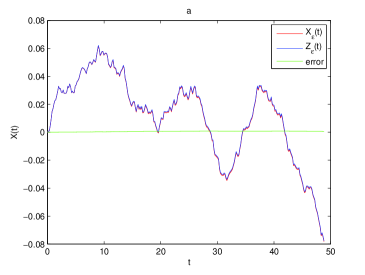
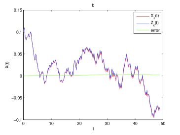
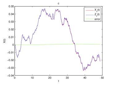
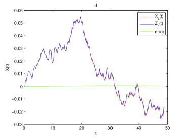
Figure 1: Comparison of the exact solution $X_{\epsilon}(t)$ with the averaged solution $Z_{\epsilon}(t)$ for equations Eq.(14) and Eq.(15) (a) $X_{0}=0.0,\lambda=0.2,\epsilon=0.045,H=0.75$ (b) $X_{0}=0.1,\lambda=0.2,\epsilon=0.045,H=0.55$ (c) $X_{0}=0.1,\lambda=0.4,\epsilon=0.01,H=0.6$ (d) $X_{0}=0.0,\lambda=0.4,\epsilon=0.02,H=0.7$

Now we carry out the numerical simulation to get the solutions of (14) and (15) under conditions of $X_{0}=0.0,\lambda=0.2,\epsilon=0.045,H=0.75$ , $X_{0}=0.1,\lambda=0.2,\epsilon=0.045,H=0.85$ ,$X_{0}=0.1,\lambda=0.4,\epsilon=0.01,H=0.6$, $X_{0}=0.0,\lambda=0.4,\epsilon=0.02,H=0.7$ respectively. Figure 1 $(a)\sim(d)$ show the comparison of exact solution $X_{\epsilon}(t)$ with averaged solution $Z_{\epsilon}(t)$ for equations (14) and (15). One can find a good agreement between solutions of the original equation and the averaged equation.

Example 2.

Consider the following SDE with the fractional Gaussian noise :

$$dX_{\epsilon}=-\epsilon^{2H}dt+\epsilon^{H}\cos^{2}(t)\lambda d^{\circ}B^{H}(t),$$ (16)

here we denote $X(0)=X_{0}$ as the initial condition with $\mathbb{E}|X(0)|^{2}<\infty$.

Here $b(t,X_{\epsilon})=-1$, and $\sigma(t,X_{\epsilon})=\cos^{2}(t)\lambda$. Now we define a new (averaged) SDE as

$$dZ_{\epsilon}=-\epsilon^{2H}dt+\frac{3}{4}\lambda\epsilon^{H}d^{\circ}B^{H}(t).$$ (17)

Obviously, all conditions in Theorem 1 and Theorem 2 are satisfied for the averaged SDE (17), so we can use the solution $Z_{\epsilon}(t)$ to approximate the original solution $X_{\epsilon}(t)$ to SDE (16), and the convergence in mean square and in probability will be assured.

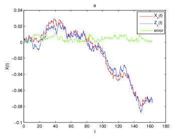
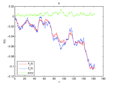
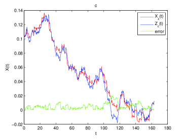
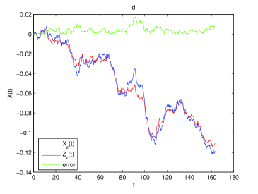
Figure 2: Comparison of the exact solution $X_{\epsilon}(t)$ with the averaged solution $Z_{\epsilon}(t)$ for equations(17).(a) $X_{0}=0.0,\lambda=2.0,\epsilon=0.001,H=0.55$ (b) $X_{0}=0.0,\lambda=2.0,\epsilon=0.0045,H=0.65$ (c)$X_{0}=0.1,\lambda=3.0,\epsilon=0.002,H=0.6$ (d)$X_{0}=0.0,\lambda=3.0,\epsilon=0.002,H=0.7$

Acknowledgments

This work was supported by the NSF of China (Grant Nos. 10972181, 11102157), Program for NCET, the Shaanxi Project for Young New Star in Science and Technology, NPU Foundation for Fundamental Research and SRF for ROCS, SEM. We thank Ilya Pavlyukevich for valuable discussions, and referees for their helpful comments.

References

- [1] R. L. Stratonovich, Topics in the Theory of Random Noise, New York, Gordon and Breach, Vol.1, 1963; Vol.2, 1967.
- [2] R. L. Stratonovich, Conditional Markov Processes and Their Application to the Theory of Optimal Control. American Elsevier, 1967.
- [3] R. Z. Khasminskii, A limit theorem for the solution of differential equations with random right-hand sides, Theory Probab.Appl. 11(1963), 390–405.
- [4] R. Z. Khasminskii, Principle of averaging of parabolic and elliptic differential equations for Markov process with small diffusion, Theory Probab.Appl.8(1)(1963) 1–21.
- [5] N. Sri. Namachchivaya and Y. K. Lin , Application of stochastic averaging for systems with high damping, Probab. Eng. Mech. 3(1988) 185–196.
- [6] J. Roberts and P. Spanos, Stochastic averaging : an approximate method of solving random vibration problems, Int.J.Non-linear Mech. 21(1986) 111–134.
- [7] R. Liptser and V. Spokoiny, On Estimating a Dynamic Function of a Stochastic System with Averaging, Statistical Inference for Stochastic Processes 3(2000): 225-249.
- [8] W. Q. Zhu, Nonlinear stochastic dynamics and control in Hamiltonian formulation, ASME Appl. Mech. Rev. 59(4)(2006)230-248.
- [9] Y. Zeng, W. Q. Zhu, Stochastic Averageing of Quasi-Nonintegrable-Hamiltonian Systems Under Poisson White Noise Excitation, J. Apple. Mech.-Trans. ASME, 78(2011)021002-021011.
- [10] W. T. Jia, W. Q. Zhu, Stochastic averaging of quasi-non-integrable Hamiltonian systems under combined Gaussian and Poisson white noise excitations, Int J Nonlin Mech, http://dx.doi.org/10.1016/j.ijnonlinmec.2012.12.003.
- [11] Y. Xu, J. Duan and W. Xu, An averaging principle for stochastic dynamical systems with Levy noise, Physica D. 240(2011), 1395–1401.
- [12] A. N. Kolmogorov, Wienersche Spiralen und einige andere interessante Kurven im Hilbertschen, Raum, C.R.(Dokaldy) Acad.Sci.URSS(N.S.). 26(1940), 115–118.
- [13] B. B. Mandelbrot and J. W. Van Ness, Fractional Brownian motions, fractional noises and applications, SIAM Review 10(4)(1968), 422–427.
- [14] N. Chakravarti and K. L. Sebastian, Fractional Brownian motion models for ploymers, Chemical Physics Letter. Vol. 267(1997), 9-13.
- [15] Y. Hu and B. Øksendal, Fractional white noise calculus and application to finance, Infin.Dimens.Anal.Quantum Probab.Relat.Topics 6(2003),1-32.
- [16] W. E. Leland, M. S. Taqqu, W. Willinger and D. V. Wilson,On the self-similar nature of ethernet traffic, IEEE/ACM Trans.Networking. 2(1994), 1-15.
- [17] R. Scheffer and F. R. Maciel, The fractional Brownian motion as a model for an industrial airlift reactor, Chemical Engineering Science. vol.56(2001), 707–711.
- [18] I. Norros, E. Valkeila and J. Virtamo, An elementary approach to a Girsanov formula and other analytivcal resuls on fractional Brownian motion, Bernoulli. 5(1999),571–587.
- [19] A. N. Shiryaev, Essentials of Stochastic Finance : Facts ,Models and Theory. World Scientific, New Jersey, 1999.
- [20] R. T. Baillie, Long memory processes and fractional integration in econometrics, Journal of Econometrics, 73(1996): 5-59.
- [21] G. Jumarie, Stochastic differential equations with fractional Brownian motion input. Int. J. Syst. Sci. 24(6)(1993), 1113–1132.
- [22] G. Jumarie, On the solution of the stochastic differential equation of exponential growth driven by fractional Brownian motion, Appl. Math. Lett. 18 (2005), 817–826.
- [23] S. C. Kou and X. S. Xie, Generalized Langevin Equation with Fractional Gaussian Noise : Subdiffusion within a Single Protein Molecule. Phys. Rev. Lett. 93(2004),180603.
- [24] O. Y. Sliusarenko, V. Y. Gonchar, A. V. Chechkin,, I. M. Sokolov and R. Metaler, Kramers-like escape driven by fractional Brownian noise, Phys. Rev. E. 81(2010), 041119.
- [25] W. Dai and C. C. Heyde, Itô formula with respect to fractional Brownian motion and its application, Journal of Appl.Math.and Stoch.Anal. 9(1996), 439–448.
- [26] L. Decreusefond and A. S. Ustunel, Fractional Brownian motion : Theory and applications, ESAIM:Proceedings 5(1998),75–86.
- [27] D. Feyel and A. de la Pradelle, Fractional integrals and Brownian processes, Potential Analysis. 10(1996), 273–288.
- [28] P. Carmona and L. Coutin, Stochastic integration with respect to fractional Brownian motion, Ann. Inst. 39(2003), 27-68.
- [29] E. Alos and D. Nualart, Stochastic calculus with respect to the fractional Brownian motion, Ann. Probab. 29(2001), 766-801.
- [30] L. C. Young, An inequality of the Holder type connected with Stieltjes integratin, Acta Math. 67(1936), 251–282.
- [31] M. Zahle, Integration with respect to fractal functions and stochastic calculus II, Math. Nachr. 225(2001),145–183.
- [32] F. Russo and P. Vallois, Forward, backward and symmetric stochastic integration, Probab. Theory Rel. Fields, 97:403–421.
- [33] F. Biagini, Y. Hu, B. Oksendal and T. Zhang, Stochastic Calculus for Fractional Brownian Motion and Applications, Springer-Verlag, London, 2008.
- [34] T. E. Duncan, Y. Hu and B. Pasik-Duncan, Stochastic calculus for fractional Brownian motion I: Theory. SIAM J. Control Optim. 38(2000) 582–612.
- [35] Y. S. Mishura, Stochastic Calculus for Fractional Brownian Motion and Related Processes, Springer-Verlag, Berlin, 2008.
- [36] T. Lyons, Differential equations driven by rough signals, Rev. Mat. Iberoamericana. 14(1998), 215–310.
- [37] D. Nualart and A. Rascanu, Differential equations driven by fractional Brownian motion, Collect. Math. 53(2002), 55-81.