Abstract

The paper is an overview of the main contributions of a Bulgarian team of researchers to the problem of finding the possible structures and waves in the open nonlinear heat conducting medium, described by a reaction-diffusion equation. Being posed and actively worked out by the Russian school of A. A. Samarskii and S.P. Kurdyumov since the seventies of the last century, this problem still contains open and challenging questions.

Structures and waves
in a nonlinear heat-conducting medium
 
Stefka Dimova,
Faculty of Mathematics and Informatics, University of Sofia, Bulgaria
dimova@fmi.uni-sofia.bg
Milena Dimova, Daniela Vasileva,
Institute of Mathematics and Informatics, Bulgarian Acad. Sci.
mkoleva,vasileva@math.bas.bg

The final publication will appear in Springer Proceedings in Mathematics and Statistics (http://www.springer.com/series/10533), Numerical Methods for PDEs: Theory, Algorithms and their Applications.

1 Introduction

A very general form of the model of heat structures reads as follows:

$$u_{t}=\sum_{i=1}^{N}(k_{i}(u)u_{x_{i}})_{x_{i}}+Q(u),\ t>0,\ x\in\mathbb{R}^{N},$$ (1)

where the heat conductivity coefficients $k_{i}(u)\geq 0$ and the heat source $Q(u)\geq 0$ are nonlinear functions of the temperature $u(t,x)\geq 0$.

Models such as (1) are studied by many researchers in various contexts. A part of this research is devoted to semilinear equations: $k_{i}(u)\equiv 1,$ $Q(u)=\lambda e^{u}$ (Frank-Kamenetskii equation) and $Q(u)=u^{\beta},$ $\beta>1$. After the pioneer work of Fujita [79], these equations and some generalizations of theirs are studied intensively by many authors, including J. Bebernes, A. Bressan, H. Brezis, D. Eberly, A. Friedman, V.A. Galaktionov, I.M. Gelfand, M.A. Herrero, R. Kohn, L.A. Lepin, S.A. Posashkov, A.A. Samarskii, J.L. Vázquez, J.J.L. Velázquez. The book [80] contains a part of these investigations and a large bibliography.

The quasilinear equation is studied by D.G. Aronson, A. Friedman, H.A. Levine, S. Kaplan, L.A. Peletier, J.L. Vázquez and others. The contributions of the Russian school are significant. The unusual localization effect of the blow-up boundary regimes is discovered by numerical experiment in the work of A.A. Samarskii and M.I. Sobol in 1963 [22]. The problem of localization for quasilinear equations with a source is posed by S.P. Kurdyumov [13] in 1974. The works of I.M. Gelfand, A.S. Kalashnikov, the scientists of the school of A.A. Samarskii and S.P. Kurdyumov are devoted to the challenging physical and mathematical problems, related with this model and its generalizations. Among them are: localization in space of the process of burning, different types of blow-up, arising of structures - traveling and standing waves, complex structures with varying degrees of symmetry. The combination of the computational experiment with the progress in the qualitative and analytical methods of the theory of ordinary and partial differential equations, the Lie and the Lie-Bäcklund group theory, has been crucial for the success of these investigations. The book [32] contains many of these results, achieved to 1986, in the review [NEW] there are citations of later works.

A special part of these investigations is devoted to finding and studying different kinds of self-similar and invariant solutions of equation (1) with power nonlinearities :

$$k_{i}(u)=u^{\sigma_{i}},\ \ Q(u)=u^{\beta}.$$ (2)

This choice is suggested by the following reasoning.

First, such temperature dependencies are usual for many real processes [25], [86], [14]. For example, when ${\sigma_{i}}={\sigma}=2.5$, ${\beta}\leq 5.2$, equation (1) describes thermo-nuclear combustion in plasma in the case of electron heat-conductivity; the parameters ${\sigma}=0$, $\ 2\leq{\beta}\leq 3$ correspond to the models of autocatalytic processes with diffusion in the chemical reactors; ${\sigma}{\approx}6.5$ corresponds to the radiation heat-conductivity of the high-temperature plasma in the stars, and so on.

Second, it is shown in [27], that in the class of power functions the symmetry of equation (1) is maximal in some sense - the equation admits a rich variety of invariant solutions. In general, almost all of the dissipative structures known so far are invariant or partially invariant solutions of nonlinear equations. The investigations of the dissipative structures provide reasons to believe that the invariant solutions describe the attractors of the dissipative structures’ evolution and thus they characterize important internal properties of the nonlinear dissipative medium.

Third, this rich set of invariant solutions of equation (1) with power nonlinearities is necessary for the successful application of the methods for investigating the same equation in the case of more general dependencies $k_{i}(u)$, $Q(u)$. By using the methods of operator comparison [48] and stationary states [47] it is possible to analyze the properties of the solutions (such as localization, blow-up, asymptotic behavior) of whole classes general nonlinear equations. The method of approximate self-similar solutions [31], developed in the works of A.A. Samarskii and V.A. Galaktionov, makes it possible to put in accordance with such general equations some other, basic equations. The latter could have invariant solutions even if the original equations do not have such. Moreover, the original equations may significantly differ from the basic equations, and nevertheless their solutions tend to the invariant solutions of the basic equations at the asymptotic stage.

Finally, in the case of power coefficients the dissipation and the source are coordinated so that complex structures arise, moreover, a spectrum of structures, burning consistently, occurs.

Below we report about the main contributions of the Bulgarian research team: S.N. Dimova,

2 The radially symmetric case, the main notions

Let us introduce the main notions to be used further on the Cauchy problem for equation (1) with initial data: u(0,x)=u_0(x)≥0,  x ∈R^N,  supu_0(x) ¡ ∞. This problem could have global or blow-up solutions. The global in time solution is defined and bounded in $\mathbb{R}^{N}$ for every t. The unbounded (blow-up) solution is defined in $\mathbb{R}^{N}$ on a finite interval $[0,T_{0})$, moreover ¯lim_t →T_0^- sup_x ∈R^N u(t,x) = +∞. The time $T_{0}$ is called blow-up time.

The unbounded solution of the Cauchy problem with finite support initial data $u_{0}(x)$ is called localized (in a strong sense), if the set Ω_L={x ∈R^N:   u(T_0^-,x):= ¯limt→T0-   u(t,x)¿0 } is bounded in $\mathbb{R}^{N}$. The set $\Omega_{L}$ is called localization region. The solution localized in a strong sense grows infinitely for $t\to T_{0}^{-}$ in a finite region ωL={x ∈RN:  u(T0-,x)= ∞} in general different from $\Omega_{L}$.

If for $k_{i}(u)\equiv 0$ the condition

$$\int_{1}^{\infty}{du\over Q(u)}<+\infty$$ (3)

holds, then the solution of the Cauchy problem is unbounded [32]. The heating of the medium happens in a blow-up regime, moreover the blow-up time of every point of the medium is different, depending on its initial temperature.

If for $Q(u)\equiv 0$ the condition

$$\int_{0}^{1}{k_{i}(u)\over u}\,du<+\infty,\ \ i=1,2,...,N,$$ (4)

holds, then a finite speed of heat propagation takes place for a finite support initial perturbation in an absolutely cold medium [32].

In the case (2) of power nonlinearities it is sufficient to have $\sigma_{i}>0,\beta>1$ for the conditions (3) and (4) to be satisfied. Then $k_{i}(0)=0$ and equation (1) degenerates. In general it has a generalized solution, which could have discontinuous derivatives on the surface of degeneration $\{u=0\}.$

2.1 The basic blow-up regimes will be explained on the radially symmetric version of the Cauchy problem for equation (1):

$$u_{t}={1\over x^{N-1}}(x^{N-1}u^{\sigma}u_{x})_{x}+u^{\beta},\quad x\in\mathbb{R}^{1}_{+},\quad t>0,\quad\sigma>0,\ \beta>1,$$ (5)

$$u_{x}(t,0)=0,\quad u(0,x)=u_{0}(x)\geq 0,\ 0\leq x<l,\quad u_{0}(x)\equiv 0,\quad x\geq l.$$ (6)

If $u_{0}(x)$ satisfies the additional conditions $u_{0}(x)\in C(\mathbb{R}_{+}^{1}),\ (u_{0}^{\sigma}u_{0}^{\prime})(0)=0,$ there exists unique local (in time) generalized solution $u=u(t,x)$ of problem (5)-(6), which is a nonnegative continuous function in $\mathbb{R}_{+}^{1}\times(0,T),$ where $T\in(0,\infty]$ is the finite or infinite time of existence of the solution (see the bibliography in the review [130]). Moreover $u(t,x)$ is a classical solution in a vicinity of every point $(t,x)$, where $u(t,x)$ is strictly positive. It could not have the necessary smoothness at the points of degeneracy, but the heat flux $-x^{N-1}u^{\sigma}u_{x}$ must be continuous. It means that $u^{\sigma}u_{x}=0$ everywhere $u=0$.

Equation (5) admits a self-similar solution (s.-s.s.) [32]:

$$u_{s}(t,x)=\varphi(t)\theta_{s}(\xi)=\left(1-{t\over T_{0}}\right)^{-1\over\beta-1}\theta_{s}(\xi),$$ (7)

$$\xi=x/\psi(t)=x/\left(1-{t\over T_{0}}\right)^{m\over{\beta-1}},\ \ m={\beta-\sigma-1\over 2}.$$ (8)

The s.-s.s. corresponds to initial data $u_{s}(0,x)=\theta_{s}(x)$. The function $\varphi(t)$ determines the amplitude of the solution. The self-similar function (s.-s.f.) $\theta_{s}(\xi)\geq 0$ determines the space-time structure of the s.-s.s. (7). This function satisfies the degenerate ordinary differential equation in $\mathbb{R}_{+}^{1}$:

$$L(\theta_{s})\equiv-{1\over\xi^{N-1}}(\xi^{N-1}\theta^{\sigma}_{s}\theta^{\prime}_{s})^{\prime}+{\beta-\sigma-1\over 2(\beta-1)T_{0}}\xi\theta^{\prime}_{s}+{1\over(\beta-1)T_{0}}\theta_{s}-\theta^{\beta}_{s}=0$$ (9)

and the boundary conditions:

$$\theta^{\prime}_{s}(0)=0,\ \ \theta_{s}(\infty)=0,\ \ \theta^{\sigma}_{s}\theta^{\prime}_{s}(\xi_{0})=0,\ \mbox{if}\ \ \theta_{s}(\xi_{0})=0.$$ (10)

Equation (9) has two constant solutions: $\theta_{s}(\xi)\equiv\theta_{H}=$ $(T_{0}(\beta-1))^{-1\over\beta-1}$ and $\theta_{s}(\xi)\equiv 0.$ These two solutions play an important role in the analysis of the different solutions of equation (9). For blow-up regimes we assume $T_{0}>0.$ Without loss of generality we set

$$T_{0}=1/(\beta-1),\ \ \mbox{then}\ \ \theta_{H}\equiv 1.$$ (11)

The analysis of the solutions of problem (9), (10), carried out in the works [36], [10], [39], [41], (see also [32], Chapter IV), gives the following results:

• For arbitrary $1<\beta\leq\sigma+1$ there exist a finite support solution $\theta_{s}(\xi)\geq 0.$

• For $\beta<\sigma+1,\ N\geq 1$ and $\beta=\sigma+1,\ N>1$ the problem has no nonmonotone solutions. The uniqueness is proved only for $\beta<\sigma+1,\ N=1.$

  The graphs of the s.-s.f. $\theta_{s}(\xi)$ for $\beta=\sigma+1=3,\ N=1,2,3$ are shown in Fig. 1, the graphs of the s.-s.f. $\theta_{s}(\xi)$ for $\beta=2.4<\sigma+1=3,\ N=1,2,3$ – in Fig. 2.

  

  

  Figure 1: $\beta=\sigma+1$, $S$-regime

  Figure 2: $\beta<\sigma+1$, $HS$-regime

• For $\beta>\sigma+1,\ N\geq 1$ the problem has no finite support solutions.

• If $\sigma+1<\beta<\beta_{s}=(\sigma+1)(N+2)/{(N-2)_{+}}$, ($\beta_{s}$ – the critical Sobolev exponent), the problem has at least one solution $\theta_{s}(\xi)>0$ in $\mathbb{R}^{1}_{+}$, strictly monotone decreasing in $\xi$ and having the asymptotics

  $$\theta_{s}(\xi)=C_{s}\xi^{-2/(\beta-\sigma-1)}[1+\omega(\xi)],\qquad\omega(\xi)\to 0,\qquad\xi\to\infty,$$ (12)

  $C_{s}=C_{s}(\sigma,\beta,N)$ is a constant. Later on in [50] the interval in $\beta$ has been extended.

• For $N=1,\ \ \beta>\sigma+1$ the problem has at least

  $$K=-[-a]-1,\ \ a={\beta-1\over\beta-\sigma-1}>1$$ (13)

  different solutions ([41], [39], [32]). Let us introduce the notations $\theta_{s,i}(\xi),\ i=1,2,\ldots,K$ for them. On the basis of linear analysis and some numerical results in the works [43], [57] it has been supposed that the number of different solutions $\theta_{s,i}(\xi)$ for $\beta>\sigma+1$ and $N\geq 1$ is $K+1.$ For $N=1$ this result was refined [132] by using bifurcation analysis: the number of solutions is $K=[a]$, if $a$ is not an integer, and $K=a-1$, if $a$ is an integer. For $N=2,3$ the bifurcation analysis gives the same estimate for the number of different solutions, but for $\beta\approx\sigma+1$, $\beta>\sigma+1$ it is violated (see 4.1).

Figure 3: $\beta>\sigma+1$, $LS$-regime

Figure 4: $\beta>\sigma+1$, $LS$-regime

The graphs of the four self-similar functions, existing for $\sigma=2,\beta=3.6>\sigma+1$ ($K=4$) are shown in Fig. 3 ($N=1$) and Fig. 4 ($N=3$).

These results determine the basic regimes of burning of the medium, described by the s.-s.s. (7), (8). The following notions are useful for their characterization:

– semi-width $x_{s}=x_{s}(t)$, determined by the equation $u(t,x_{s})=u(t,0)/2$ for solutions, monotone in $x$ and having a single maximum at the point $x=0$;

– front-point $x_{f}$: $u(t,x_{f})=0,\ \ u^{\sigma}u_{x}(t,x_{f})=0.$

2.1.1 $HS$-evolution, total blow-up, $1<\beta<\sigma+1$

The heat diffusion is more intensive than the heat source. The semi-width and the front tend to infinity; a heat wave, which covers the whole space for time $T_{0},$ is formed. The process is not localized: $\displaystyle{\rm mes}\ \Omega_{L}={\rm mes}\ \omega_{L}=\infty,\ \ x_{s}\to\infty,\ \ x_{f}\to\infty,\ \ t\to T^{-}_{0}.$

2.1.2 $S$-evolution, regional blow-up, $\beta=\sigma+1$

The heat diffusion and the source are correlated in such a way, that leads to localization of the process in a region $\Omega_{L}=\omega_{L}=\left\{|x|<{L_{s}/2}\right\}$ of diameter $L_{s},$ called a fundamental length of the $S$-regime. The semi-width is constant, inside $\Omega_{L}$ the medium is heated to infinite temperature for time $T_{0}:\ x_{s}={\rm const},\ x_{f}=L_{s}/2.$ In the case $N=1$ the solution $\theta_{s}(\xi)$ (Zmitrenko-Kurdyumov solution) is found [10] explicitly:

$$\theta_{s}(\xi)=\left\{\begin{array}[]{ll}\displaystyle\left({2(\sigma+1)\over\sigma+2}\cos^{2}{\pi\xi\over L_{s}}\right)^{1/\sigma},&\displaystyle|\xi|\leq{L_{s}\over 2}\\ 0&\displaystyle|\xi|>{L_{s}\over 2},\end{array}\right.$$ (14)

$L_{s}={\rm diam}\ \Omega_{L}=(2\pi\sqrt{\sigma+1})/\sigma,\ \ x_{s}=L_{s}\arccos((2^{-{\sigma\over 2}})/\pi).$

The solution (14) is called elementary solution of the $S$-regime for $N=1$. In this case equation (9) is autonomous and every function, consisting of $k$ elementary solutions, $k=1,2,\ldots$, is a solution as well, i.e., equation (9) has a countable set of solutions.

2.1.3 $LS$-evolution, single point blow-up, $\sigma+1<\beta<\beta_{f}=\sigma+1+{2\over N}$

Here $\beta_{f}$ is the critical Fujita exponent [81]. The intensity of the source is bigger, than the diffusion. The front of the s.-s.s. is at infinity (12), the semi-width decreases and the medium is heated to infinite temperature in a single point: mes  ωL=0,  xs →0,  t→T-0. According to the different s.-s.f. $\theta_{s,i}(\xi),\ i=1,2,\ldots,$ the medium burns as a simple structure $(i=1)$ and as complex structures $(i>1)$ with the same blow-up time.

2.2 Stability of the self-similar solutions

To show the important property of the s.-s.s. as attractors of wide classes of other solutions of the same equation, we will need of additional notions.

In the case of arbitrary finite support initial data $u_{0}(x)$ (6) the so called self-similar representation [39] of the solution $u(t,x)$ of problem (5), (6) is defined. It is determined at every time $t$ according to the structure of the s.-s.s. (7), (8):

$$\Theta(t,\xi)=\left(1-{t/T_{0}}\right)^{1\over\beta-1}u\left(t,\xi\left(1-{t/T_{0}}\right)^{m\over\beta-1}\right)=\varphi^{-1}(t)u(t,\xi\psi(t)).$$ (15)

The s.-s.s. $u_{s}(t,x)$ is called asymptotically stable [32], if there exists a sufficiently large class of solutions $u(t,x)$ of problem (5), (6) for initial data $u_{0}(x)\not\equiv\theta_{s}(x)$, whose self-similar representations $\Theta(t,\xi)$ tend in some norm to $\theta_{s}(\xi)$ when $t\to T_{0}^{-}$:

$$\|\Theta(t,\xi)-\theta_{s}(\xi)\|\to 0,\ t\to T^{-}_{0}.$$ (16)

The definition of the self-similar representation (15) contains the blow-up time $T_{0}.$ For theoretical investigations this is natural, but for numerical investigations definition (15) is unusable since for arbitrary initial data $u_{0}(x)\neq\theta_{s}(x)$ $T_{0}$ is not known. Therefor another approach has been proposed and numerically implemented (for $N=1$) in [36], [39]. This approach gives a possibility to investigate the structural stability of the unbounded solutions in a special “self-similar” norm, consistent for every $t$ with the geometric form of the solution and not using explicitly the blow-up time $T_{0}$. A new self-similar representation, consistent with the structure of the s.-s.s. (7), (8) is introduced:

$$\Theta(t,\xi)=u(t,\xi(\gamma(t))^{-m})/\gamma(t),\qquad\gamma(t)={{\max_{x}}u(t,x)\over{\max_{\xi}}\theta_{s}(\xi)}.$$ (17)

If the limit (16) takes place for $\Theta(t,\xi)$, given in (17), then the self-similar solution $u_{s}(t,x)$ is called structurally stable.

The notion of structural stability, i.e., the preservation in time of some characteristics of the structures, such as geometric form, rate of growth, localization in space, is tightly connected with the notion invariance of the solutions with respect to the transformations, involving the time [33]. This determines its advisability for investigating the asymptotic behavior of the blow-up solutions.

In the case of complex structures another notion of stability is needed, namely metastability. The self-similar solution $u_{s}(t,x)$ is called metastable, if for every $\varepsilon>0$ there exists a class of initial data $u(0,x)\approx\theta_{s}(x)$ and a time $T$, $T_{0}-T\ll T_{0}$ such that ∥Θ(t,ξ)-θs(ξ)∥≤ε,   for  0≤t≤T holds for the self-similar representations (17) of the corresponding solutions. This means, that the metastable s.-s.s. preserves its complex space-time structure during the evolution up to time $T$, very close to the blow-up time $T_{0}$. After that time the complex structure could degenerate into one or several simple structures.

3 Numerical methods

To solve the reaction-diffusion problem (5), (6) and the corresponding self-similar problem (9), (10), as well as their generalizations both for systems of such equations and for the 2D case, appropriate numerical methods and algorithms were developed.

The difficulties, common for the nonstationary and for the self-similar problems were: the nonlinearity, the dependence on a number of parameters (not less than 3); insufficient smoothness of the solutions on the degeneration surface, where the solutions vanish. In the case of radial symmetry for $N>1$ and polar coordinates in the 2D case additional singularity at $x=0\ (\xi=0)$ occurs.

The main challenge in solving the self-similar problems is the non-uniqueness of their solutions for some ranges of the parameters. The following problems arise: to find a “good” approximation to each of the solutions; to construct an iteration process, converging fast to the desired solution (corresponding to the initial approximation) and ensuring sufficient accuracy; to construct a computational process, which enables finding all different solutions for given parameters $(\sigma,\beta,N)$ in one and the same way; to determine in advance where to translate the boundary conditions from infinity, for example (10), for the asymptotics (12) to be fulfilled.

The main difficulty in solving the nonstationary problems is the blow-up of their solutions: blow-up in a single point, in a finite region and in the whole space. And two others, related with it: the moving front of the solution, where it is often not sufficiently smooth; the instability of the blow-up solutions.

3.1 Initial approximations to the different s.-s.f. for a given set of parameters

To overcome the difficulty with the initial approximations to the different s.-s.f., we have used the approach, proposed and used in the works [43], [57]. Based on the hypothesis that in the region of their nonmonotonicity the s.-s.f. have small oscillations around the homogenious solution $\theta_{H},$ this approach consists of “linearization” of the self-similar equation around $\theta_{H}$ and followed by “sewing” the solutions of the resulting linear equation with the known asymptotics at infinity, e.g. (12).

Our experiments showed [D09], that when $\beta\to\sigma+1+0$ the hypothesis about small oscillations of the s.-s.f. around $\theta_{H}$, is not fulfilled. The detailed analytical and numerical investigations [D09], [D11], [D25] of the “linear approximations” in the radially symmetric case for $N=1,2,3,$ showed that even in the case these approximations take negative values in vicinity of the origin, they still give the true number of crossings with $\theta_{H}$ and thus, the character of nonmonotonicity of the s.-s. functions. Recommendations of how to use the linear approximations in these cases are made in [D09].

Let us note, the “linear approximations” are expressed by different special functions: the confluent hypergeometric function ${}_{1}F_{1}(a,b;z)$ and the Bessel function $J_{k}(z)$ for different parameter ranges within the complex plane for $a$ and $b$ and different ranges of the variable $z$. To compute these special functions, various methods were used: Taylor series expansions, expansions in ascending series of Chebyshev polynomials, rational approximations, asymptotic series [D16], [D24].

3.2 Numerical method for the self-similar problems

To solve the self-similar problem (9), (10) and its generalization for systems of ODE and for the 2D-case, the Continuous Analog of the Newton’s Method (CANM) was used ([D25]-[D09], [D11], [136], [D14]). Proposed by Gavurin [59], this method was further developed in [60], [62] and used for solving many nonlinear problems. The idea behind it is to reduce the stationary problem $L(\theta)=0$ to the evolution one:

$$L^{\prime}(\theta)\frac{\partial\theta}{\partial t}=-L(\theta),\quad\theta(\xi,0)=\theta_{0}(\xi),$$ (18)

by introducing a continuous parameter $t$, $0<t<\infty$, on which the unknown solution depends: $\theta=\theta(\xi,t)$. By setting $v=\partial\theta/\partial t$ and applying the Euler’s method to the Cauchy problem (18), one comes to the iteration scheme:

$$L^{\prime}(\theta_{n})v_{n}=-L(\theta_{n}),$$ (19)

$$\begin{array}[]{l}\theta_{n+1}=\theta_{n}+\tau_{n}v_{n},\quad 0<\tau_{n}\leq 1,\quad n=0,1,\dots,\\[3.0pt] \theta_{n}=\theta_{n}(\xi)=\theta(\xi,t_{n}),\quad v_{n}=v_{n}(\xi)=v(\xi,t_{n}),\\[3.0pt] \qquad\theta_{0}(\xi)\ \mbox{being the initial approximation}.\end{array}$$ (20)

The linear equations (19) (or the system of such equations in the case of a two-component medium) are solved by the Galerkin Finite Element Method (GFEM) at every iteration step. The combination of the CANM and the GFEM turned out to be very successful. The linear system of the FEM with nonsymmetric matrix is solved by using the $LU$ decomposition. The iteration process (20) converges very fast – usually less than 15-16 iterations are sufficient for stop-criterium $\|L(\theta_{n})\|<10^{-7}$. The numerical investigation of the accuracy of the method being implemented shows errors (i) of order $O(h^{4})$ when using quadratic elements in the radially symmetric case, and (ii) of optimal order $O(h^{2})$ when using linear elements in the same case or bilinear ones in the 2D case. To achieve the same accuracy in vicinity of the origin in the radially symmetric case for $N\geq 3$ the nonsymmetric Galerkin method [84] was developed [D11], [D23].

The computing of the solutions of the linearized self-similar equation and their sewing with the known asymptotics is implemented in a software, so the process is fully automatized. The software enables the computing of the self-similar functions for all of the blow-up regimes, moreover in the case of $LS$-regime only the number $k$ of the self-similar function $\theta_{s,k}(\xi)$ must be given.

3.3 Numerical method for the reaction-diffusion problems

The Galerkin Finite Element Method (GFEM), based on the Kirchhoff transformation of the nonlinear heat-conductivity coefficient:

$$G(u)=\int_{0}^{u}{s^{\sigma}}\,ds=u^{\sigma+1}/(\sigma+1),$$ (21)

was used ([D01], [D03], [D16], [D25]-[D26], [D18]-[D21], [D19], [78]) for solving the reaction-diffusion problems. This transformation is crucial for the further interpolation of the nonlinear coefficients on the basis of the finite element space and for optimizing of the computational process.

Here below we point out the main steps of the method on the problem (5), (6) in a finite interval [0, $X(t)$] under the boundary condition $u(X(t))=0$. Because of the finite speed of heat propagation we choose $X=X(t)$ so as to avoid the influence of the boundary condition on the solution. The discretization is made on the Galerkin form of the problem:

Find a function $u(t,x)\in D,$ D={u: x(N-1)/2u,  x(N-1)/2 ∂u(σ+1)/2/ ∂x ∈L2,  u(X(t))=0 }, which for every fixed $t$ satisfies the integral identity

$$(u_{t},v)=A(t;u,v),\quad\forall v\in H^{1}(0,X(t)),\ \ \ 0<t<T_{0},$$ (22)

and the initial condition (6).

Here (u,v)=∫X(t)0 xN-1 u(x) v(x)dx,    A(t;u,v)=∫X(t)0 [xN-1 ∂G(u)∂x ∂v∂x + x uβv]dx, H1 (0,X(t))={v:x(N-1)/2 v,  x(N-1)/2 v’∈L2(0,X(t)),  v(X(t))=0. } The lumped mass finite element method [97] with interpolation of the nonlinear coefficients $G(u)$ (21) and $q(u)=u^{\beta}$: G(u) ∼GI=∑ni=1 G(ui)φi(x),   q(u) ∼qI=∑ni=1 q(ui)φi(x) on the basis $\{\varphi_{i}\},i=1,\dots,n,$ of the finite element space is used for discretization of (22). The resulting system of ordinary differential equations with respect to the vector $U(t)=(u_{1}(t),u_{2}(t),\ldots,u_{n}(t))^{T}$ of the nodal values of the solution $u(t,x)$ at time $t$ is:

$$\dot{U}=\tilde{M}^{-1}(-KG(U))+q(U),\quad U(0)=U_{0}.$$ (23)

Here the following denotations are used: $G(U)=(G(u_{1}),\ldots,G(u_{n}))^{T},\quad q(U)=(q(u_{1}),\ldots,q(u_{n}))^{T},$ $\tilde{M}$ is the lumped mass matrix, $K$ is the stiffness matrix. Let us mention, thanks to the Kirchhoff transformation and the interpolation of the nonlinear coefficients only the two vectors $G(U)$ and $q(U)$ contain the nonlinearity of the problem, while the matrix $K$ does not depend on the unknown solution.

To solve the system (23) an explicit Runge-Kutta method [66] of second order of accuracy and an extended region of stability was used. A special algorithm for choosing the time-step $\tau$ ensures the validity of the weak maximum principle and, in the case of smooth solutions, the achievement of a given accuracy $\epsilon$ up to the end of the time interval. The stop criterion is $\tau<10^{-16}$ and then $\tilde{T}_{0}$ is the approximate blow-up time, found in the computations.

It is worth mentioning, that the nonlinearity has changed the prevailing opinion about the explicit methods. Indeed, there are at least two reasons an explicit method to be preferred over the implicit one for solving the system (23):

– the condition for solvability of the nonlinear discrete system on the upper time level imposes the same restriction on the relation ”time step – step in space”, as does the condition for validity of the weak maximum principle for the explicit scheme (see [32], chapter VII, §5);

– the explicit method for solving large discrete systems has a significant advantage over the implicit one with respect to the computational complexity.

Let us also mention, that in the case of blow-up solutions the discrete system on the upper time level would connect solution values differing by 6-12 orders of magnitude, which causes additional difficulties to overcome. Finally the explicit methods allow easy parallelization.

The special achievement of the proposed methods are the adaptive meshes in the $LS$-regime (refinement of the mesh) and in the $HS$-regime (stretching meshes with constant number of mesh-points), consistent with the self-similar low. Let us briefly describe this adaptation idea on the differential problem

$$u_{t}=Lu,\ \ u=u(t,x),\ \ x\in\mathbb{R^{N}},\ \ t>0,$$ (24)

which admits a self-similar solution of the kind

$$u_{s}(t,x)=\varphi(t)\theta_{s}(\xi),\qquad\xi={x}/{\psi(t)},\ \ u_{s}(0,x)=\theta_{s}(x).$$ (25)

Since the invariant solution $u_{s}(x,t)$ is an attractor of the solutions of equation (24) for large classes of initial data different from $\theta_{s}(x)$, it is important to incorporate the structure (25) in the numerical method for solving equation (24). The relation (25) between $\xi$ and $x$ gives the idea how to adapt the mesh in space. Let $\Delta x^{(0)}$ be the initial step in space, $\Delta x^{(k)}$ – the step in space at $t=t^{k}$. Then $\Delta x^{(k)}$ must be chosen so that $\Delta\xi^{(k)}$ is bounded from below and from above Δx(0) / λ ≤Δξ(k) ≤ λΔx(0) for an appropriate $\lambda$ (usually $\lambda=2$).

Further, by using the relation between $\psi(t)$ and $\varphi(t)$, it is possible to incorporate the structure (25) of the s.-s.s. in the adaptation procedure. In the case of equation (5) we have

$$\xi=x{\Gamma(t)}^{m},\quad\Delta\xi=\Delta x{\Gamma(t)}^{m},\quad m={{(\beta-\sigma-1)}/{2}},\quad\Gamma(t)=\frac{\max_{x}u(t,x)}{\max_{x}u_{0}(x)}.$$ (26)

On the basis of the relations (26) the following strategy is accepted.

In the case of a single point blow-up, $m>0$, we choose the step $\Delta x^{(k)}$ so that the step $\Delta\xi^{(k)}$ be bounded from above:

$$\Delta\xi^{(k)}=\Delta x^{(k)}{\Gamma(t)}^{m}\leq{\lambda\Delta x^{(0)}}.$$ (27)

When condition (27) is violated, the following procedure is carried out: every element in the region, in which the solution is not established with a given accuracy $\delta_{u}$ (usually $\delta_{u}=10^{-7}$), is divided into two equal elements and the values of the solution in the new mesh points are found by interpolating from the old values; the elements, in which the solution is established with a given accuracy $\delta_{u}$, are neglected.

In the case of a total blow-up, $m<0$, we choose the step $\Delta x^{(k)}$ so that the step $\Delta\xi^{(k)}$ be bounded from below:

$$\Delta\xi^{(k)}=\Delta x^{(k)}{\Gamma(t)}^{m}\geq{\lambda\Delta x^{(0)}}.$$ (28)

When condition (28) is violated, the lengths of the elements are doubled, and so is the interval in $x$: $X(t_{k+1})=2X(t_{k})$, thus the number of mesh points remains constant.

This adaptation procedure makes it possible to compute efficiently the single point blow-up as well as the total blow-up solutions up to amplitudes $10^{6}-10^{12},$ depending on the medium parameters. It ensures the authenticity of the results of investigation of the structural stability and the metastability of the self-similar solutions. Let us note, this approach does not require an auxiliary differential problem for the mesh to be solved, unlike the moving mesh methods [1100]. The idea to use the invariant properties of the differential equations and their solutions [114] and to incorporate the structural properties (e.g. geometry, different kind of symmetries, the conservation laws) of the continuous problems in the numerical method, lies at the basis of an important direction of the computational mathematics - geometric integration, to which many works and monographs are devoted - see [70], [68], [69] and the references therein.

The numerous computational experiments carried out with the exact self-similar initial data (14) for $N=1,\beta=\sigma+1,$ as well as with the computed self-similar initial data, show a good blow-up time restoration (set into the self-similar problem) in the process of solving the reaction-diffusion problem. The preservation of the self-similarity and the restoration of the blow-up time demonstrate the high quality of the numerical methods for solving both the self-similar and the nonstationary problems.

4 Results and achievements

The developed numerical technique was used to analyze and solve a number of open problems. Below we present briefly some of them.

4.1 The transition $LS$- to $S$-regime in the radially symmetric case

The investigation of the limit case $\beta\to\sigma+1+0$ resolved the following paradox for $N>1$: there exists one simple-structure s.-s. function in $S$-regime $(\beta=\sigma+1),$ whereas in $LS$-regime for $\beta\to\sigma+1+0$ their number tends to infinity according to formula (13). The detailed numerical experiment in [D11], [D09] yielded the following results. First, it was shown, that the structure of the s.-s.f. for $N>1$ and $\beta\sim\sigma+1,\ \beta>\sigma+1$ is substantially different from the one for $N=1.$ Second, for $N=1$ the transition $\beta\to\sigma+1+0$ is “continuous” – the self-similar function $\theta_{s,k}(\xi)$ for the $LS$-regime tends to a s.-s.f. of the $S$-regime, consisting of $k$ elementary solutions. For $N>1$ the transition behaves very differently.

Figure 5: Graphs of the s.-s.f. $\theta_{s,2}$ for $N=3,\ \sigma=2,\ \beta=\{3.6(1);\ 3.38(2);\ 3.2(3);\ 3.08(4);\ 3.03(5)\}$ (left) and $\theta_{s,3}$ for $N=3,\ \sigma=2,\ \beta=\{3.2(1);\ 3.1(2);\ 3.08(3);\ 3.06(4);\ 3.03(5)\}$ (right).

For $\sigma$ fixed and $\beta\to\sigma+1+0$ the central minimum of the ”even” s.-s.f. $\theta^{(N)}_{2j},\ j=1,2,\ldots,$ decreases and surprisingly becomes zero for some $\beta=\beta_{j}^{*}(\sigma,N)$ (Fig. 5, left). For $\beta<\beta_{j}^{*}(\sigma,N)$ all of the s.-s.f. have zero region around the center of symmetry, and the radius of this region tends to infinity for $\beta\to\sigma+1+0$. All of the maxima of $\theta^{(N)}_{s,2j}(\xi)$ tend to the maximum of the s.-s.f. of the $S$-regime for the corresponding $\sigma$ and for $N=1.$ Thus the s.-s.f. $\theta^{(N)}_{s,2j}(\xi),$ “going to infinity” when $\beta\to\sigma+1+0$, tends to a s.-s.f. of the $S$-regime for $N=1$ and the same $\sigma$, consisting of $j$ elementary solutions.

For fixed $\sigma$ there exists such a value $\beta^{**}_{j}(\sigma,N)$, that for $\sigma+1<\beta<\beta^{**}_{j}$ the ”odd” s.-s.f. $\theta^{(N)}_{s,2j+1}(\xi),j=1,2,\ldots$ split into two parts: a central one, tending to the s.-s.f. of the $S$-regime for the same $N$, and second one, coinciding with the s.-s.f. $\theta^{(N)}_{s,2j}(\xi),$ “going to infinity” when $\beta\to\sigma+1+0$ (Fig. 5, right).

According to the described “scenario”, when $\beta\to\sigma+1+0$ only the first s.-s.f. of the $LS$-regime remains, and it tends to the unique s.-s.f. of the $S$-regime.

As a result of this investigation new-structure s.-s.f. were found – s.-s.f. with a left front. The existence of such s.-s.functions was confirmed by an asymptotic analysis, i.e., the asymptotics in the neighborhood of the left front-point was found analytically [D25]. This new type of solutions initiated investigations of other authors [74], [132] by other methods (the method of dynamical analogy, bifurcation analysis). Their investigations confirmed our results.

4.2 The asymptotic behavior of the blow-up solutions of problem (5), (6) beyond the critical Fujita exponent

For $\beta>\beta_{f}=\sigma+1+{2/N}$ the problem (5), (6) could have blow-up- or global solutions depending on the initial data. For the s.-s. blow-up solution (7), (8) it holds $u_{s}(t,r)\not\in L_{1}(\mathbb{R}^{N})$. The qualitative theory of nonstationary averaging “amplitude-semi-width” predicts a self-similar behavior of the amplitude of the blow-up solutions and a possible non-self-similar behavior of the semi-width [32]. A question was posed there: what kind of invariant or approximate s.-s.s. describes the asymptotic stage $(t\to T^{-}_{0})$ of the blow-up process?

The detailed numerical experiment carried out in [D19], [78] showed that the s.-s.s. (7), (8), corresponding to $\theta_{s,1}(\xi)$, is structurally stable: all of the numerical experiments with finite-support initial data (6), ensuring blow-up, yield solutions tending to the self-similar one on the asymptotic stage.

4.3 Asymptotically self-similar blow-up beyond some other critical exponents

The numerical investigation of the blow-up processes in the radially symmetric case for high space-dimensions $N$ was carried out in [D22], [D23]. The aim was to check some hypotheses [50] about the solutions of the s.-s. problem (9), (10) and about the asymptotic stability of the corresponding s.-s. solutions for parameters beyond the following critical exponents:

$\beta_{s}=(\sigma+1)(N+2)/(N-2),\ N\geq 3$  (Sobolev’s exponent);

$\beta_{u}=(\sigma+1)(1+4/(N-4-2\sqrt{N-1})),\ N\geq 11;$

$\beta_{p}=1+{3(\sigma+1)+(\sigma^{2}(N-10)^{2}+2\sigma(5\sigma+1)(N-10)+9(\sigma+1)^{2})^{1/2}}/(N-10),$ $N\geq 11.$

Self-similar functions, monotone in space, were constructed numerically for all of these cases, thus confirming the hypotheses of their existence (not proved for $\beta>\beta_{u}$). It was also shown, that the corresponding s.-s.s. are structurally stable, thus confirming another hypothesis of [50]. Due to the strong singularity at the origin, the nonsymmetric Galerkin method and the special refinement of the finite element mesh [D23] were crucial for the success of these investigations.

4.4 Two-component nonlinear medium

The methods, developed for the radially symmetric problems (5), (6) and (9), (10) were generalized in [D20], [136], [78] for the case of two-component nonlinear medium, described by the system:

$$\left|\begin{array}[]{l}\displaystyle u_{1t}={1\over x^{N-1}}(x^{N-1}u_{1}^{\sigma_{1}}u_{1x})_{x}+u_{1}^{\beta_{1}}u_{2}^{\gamma_{2}},\quad x\in\mathbb{R}^{1}_{+},\ N=1,2,3,\\[10.0pt] \displaystyle u_{2t}={1\over x^{N-1}}(x^{N-1}u_{2}^{\sigma_{2}}u_{2x})_{x}+u_{1}^{\gamma_{1}}u_{2}^{\beta_{2}},\quad\sigma_{i}>0,\ \beta_{i}>1,\ \gamma_{i}\geq 0,i=1,2.\end{array}\right.$$ (29)

This system admits blow-up s.-s.s. of the form

$$\begin{array}[]{ll}\displaystyle u_{1s}=(1-{t/T_{0}})^{m_{1}}\theta_{1s}(\xi),&\xi=x/(1-{t/T_{0}})^{n},\\[10.0pt] \displaystyle u_{2s}=(1-{t/T_{0}})^{m_{2}}\theta_{2s}(\xi),&m_{i}<0,\ i=1,2,\end{array}$$ (30)

where mi=αip,  αi=γi+1-βi, i=1,2,    p=(β1-1)(β2-1)-γ1γ2, n=m1σ1+12 = m2σ2+12,   σ1(γ2+1-β2)=σ2(γ1+1-β1). The s.-s.f. satisfy the system of nonlinear ODE:

$$\left|\begin{array}[]{l}L_{1}(\theta_{1s},\theta_{2s})\equiv-{1\over\xi^{N-1}}(\xi^{N-1}\theta_{1s}^{\sigma_{1}}\theta^{\prime}_{1s})^{\prime}+n\xi\theta^{\prime}_{1s}-m_{1}\theta_{1s}-\theta_{1s}^{\beta_{1}}\theta_{2s}^{\gamma_{2}}=0,\\[10.0pt] L_{2}(\theta_{1s},\theta_{2s})\equiv-{1\over\xi^{N-1}}(\xi^{N-1}\theta_{2s}^{\sigma_{2}}\theta^{\prime}_{2s})^{\prime}+n\xi\theta^{\prime}_{2s}-m_{2}\theta_{2s}-\theta_{1s}^{\gamma_{1}}\theta_{2s}^{\beta_{2}}=0\end{array}\right.$$ (31)

and the boundary conditions

$$\lim_{\xi\to 0}\xi^{N-1}\theta_{is}^{\sigma_{1}}\theta^{\prime}_{is}=0,\ \ \lim_{\xi\to\infty}\theta_{is}=0,\ \ i=1,2.$$ (32)

Superconvergence of the FEM (of order $O(h^{4})$) for solving the s.-s. problem (31)–(32) by means of quadratic elements and optimal-order convergence ($O(h^{2})$) by means of linear elements were achieved. The structural stability of the s.-s.s. (30) for parameters $\sigma_{i},\ \beta_{i},\ \gamma_{i},\ i=1,2,$ corresponding to the $LS$-regime ($n>0$) was analyzed in [136], [78], [D20]. It was shown that only the s.-s.s. of systems (29) with strong feedback ($p<0$), corresponding to the s.-s.f. with two simple-structure components, were structurally stable. All the other s.-s.s. were metastable – self-similarity was preserved to times not less than $99.3\%\tilde{T}_{0}$.

The proposed computational technique can be applied to investigating the self-organization processes in wide classes of nonlinear dissipative media described by nonlinear reaction-diffusion systems.

4.5 Directed heat diffusion in a nonlinear anisotropic medium

Historically the first Bulgarian contribution to the topic under consideration was the numerical realization of the self-similar solutions, describing directed heat diffusion and burning of a two-dimensional nonlinear anisotropic medium. It was shown in [27] that the model of heat structures in the anisotropic case

$$u_{t}=(u^{\sigma_{1}}u_{x_{1}})_{x_{1}}+(u^{\sigma_{2}}u_{x_{2}})_{x_{2}}+u^{\beta},\ x=(x_{1},x_{2})\in\mathbb{R}^{2},\ \sigma_{1}>0,\ \ \sigma_{2}>0,\ \ \beta>1$$ (33)

admits invariant solutions of the kind us(t,x1,x2)=(1-tT0)-1β-1 θs(ξ),  ξ=(ξ1,ξ2)∈R2, ξi=xi / (1-tT0)miβ-1,  mi=β-σi-12,  i=1,2. The self-similar function $\theta_{s}(\xi_{1},\xi_{2})$ satisfies the nonlinear elliptic problem

$$L(\theta_{s})\equiv\sum^{2}_{i=1}\left(-{\partial\over\partial\xi_{i}}\left(\theta_{s}^{\sigma_{i}}{\partial\theta_{s}\over\partial\xi_{i}}\right)+{\beta-\sigma_{i}-1\over 2}\xi_{i}{\partial\theta_{s}\over\partial\xi_{i}}\right)+\theta_{s}-\theta_{s}^{\beta}=0,$$ (34)

$${\partial\theta_{s}\over\partial\xi_{i}}\Biggl{.}\Biggr{|}_{\xi_{i}=0}=0,\ i=1,2;\ \ \theta_{s}(\xi)\to 0,\ \ |\xi|\to\infty.$$ (35)

The Cauchy problem for equation (33) was investigated in the works [D01], [D03] for different parameters $\sigma_{1},\sigma_{2}$ and $\beta$. Depending on the parameters, different mixed regimes: $S-HS,\ HS-LS,\ S-LS$ of heat transfer and burning were implemented numerically. The evolution in time of one and the same initial perturbation is shown for the cases of the 2D radially symmetric $S$-regime (Fig. 6), the mixed $HS-S$-regime (Fig. 7) and the mixed $HS-LS$-regime (Fig. 8).

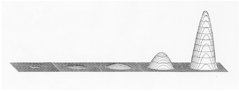
Figure 6: $S$-regime: $\sigma_{1}=2,\ \sigma_{2}=2,\ \beta=3.$

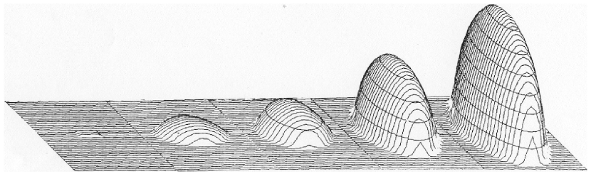
Figure 7: $HS-S$-regime: $\sigma_{1}=3,\ \sigma_{2}=2,\ \beta=3.$

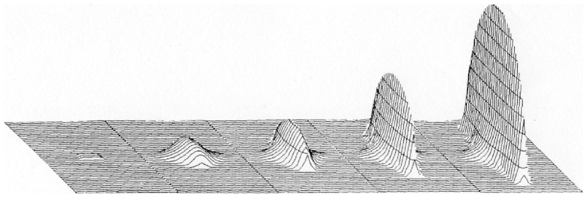
Figure 8: $HS-LS$-regime: $\sigma_{1}=3,\ \sigma_{2}=1,\ \beta=3.$

To solve the Cauchy problem for equation (33) a modification of the TERMO Package of Applied Programs [104], designed initially for solving isotropic problems with piecewise constant coefficients, was done. TERMO had been worked out by an IMI-BAS team, after the idea of Raytcho Lazarov and under his guidance, a merit worth mentioning here.

The s.-s.functions for the corresponding mixed regimes were found in [D01] by self-similar processing of the solution of the Cauchy problem for equation (33). Later, in [D06], they were found as solutions of the self-similar problem (34), (35). The self-similar functions of complex symmetry for the isotropic case in Cartesian coordinates (denoted in [57] as $Ei/j$) were found as a special case.

Later on, in [D14], [136], the numerical methods were modified for the isotropic 2D self-similar problem in polar coordinates to construct numerically another class of self-similar functions of complex symmetry (denoted in [57] as $EjMm$) in $LS$-regime and to investigate their structural stability.

Graphical representations of the evolution of the anisotropic invariant solutions, as well as the s.-s. functions $EjMm$ for some different values of $j,m,\sigma,\beta$, are included in the Handbook [85]. We show some of the s.-s.f. $EjMm$ in Fig. 9.

Figure 9: Self-similar functions EjMm, $j=1,\ m=2,3,4,5,6,7,\$ $\sigma=2,\ \beta=3.25$.

4.6 Spiral waves in $HS$-regime

The numerical realization of the invariant solutions, describing “spiral” propagation of the nonhomogeneities in two-dimensional isotropic medium appears to be one of the most interesting contributions of ours. The mathematical model in polar coordinates reads:

$$u_{t}={1\over r}(ru^{\sigma}u_{r})_{r}+{1\over r^{2}}(u^{\sigma}u_{\varphi})_{\varphi}+u^{\beta},\ \sigma>0,\ \beta>1.$$ (36)

It admits s.-s.s. of the kind [D03], [33]:

$$u_{s}(t,r,\varphi)=\left(1-{t\over T_{0}}\right)^{-{1\over\beta-1}}\theta_{s}(\xi,\phi),$$ (37)

$$\xi=r/\left(1-{t\over T_{0}}\right)^{m\over{\beta-1}},\ \ \phi=\varphi+{c_{0}\over\beta-1}\ln\left(1-{t\over T_{0}}\right),\ \ m={\beta-\sigma-1\over 2}.$$ (38)

The self-similar function $\theta_{s}(\xi,\phi)$ satisfies the nonlinear elliptic equation

$$\begin{array}[]{ll}\displaystyle L(\theta_{s})\equiv&-\displaystyle{1\over\xi}\displaystyle{\partial\over\partial\xi}\left(\xi\theta_{s}^{\sigma}{\partial\theta_{s}\over\partial\xi}\right)-{1\over\xi^{2}}{\partial\over\partial\phi}\left(\theta^{\sigma}_{s}{\partial\theta_{s}\over\partial\phi}\right)+{\beta-\sigma-1\over 2}\xi{\partial\theta_{s}\over\partial\xi}\\ \displaystyle&-\displaystyle c_{0}{\partial\theta_{s}\over\partial\phi}+\theta_{s}-\theta_{s}^{\beta}=0,\ \ \ T_{0}={1\over\beta-1}.\end{array}$$ (39)

Here $c_{0}\not=0$ is the parameter of the family of solutions. From (38) it follows ξesϕ=r esφ=const,   s=β-σ-12c0. This means, that the trajectories of the nonhomogeneities in the medium (say local maxima) are logarithmic spirals for $\beta\not=\sigma+1$ or circles for $\beta=\sigma+1.$ The direction of movement for fixed $c_{0}$, for example $c_{0}>0,$ depends on the relation between $\sigma$ and $\beta:$ for $\beta>\sigma+1$ – towards the center (twisting spirals), for $\beta<\sigma+1$ – from the center (untwisting spirals).

The problem for the numerical realization of the spiral s.-s.s. (37), (38) was posed in 1984, when the possibility for their existence has been established by the method of invariant group analysis in the PhD Thesis of S.R. Svirshchevskii. As it was stated in [82], there were significant difficulties for finding such solutions. First, the linearization of the self-similar equation (39) was not expected to give the desired result, because it is not possible to separate the variables in the linearized equation. Second, the asymptotics at infinity of the solutions of the self-similar equation were not known.

The first successful step was the appropriate (complex) separation of variables in the linearized equation. Using the assumption for small oscillations of the s.-s.f. $\theta_{s}(\xi,\phi)$ around $\theta_{H}^{1}\equiv 1$, i. e., $\theta_{s}(\xi,\phi)=1+\alpha y(\xi,\phi),\ \ \alpha=\mbox{const},\ \ |\alpha y|\ll 1$ and the idea of linearization around it, the following linear equation for $y(\xi,\phi)$ was found [D16]: -1ξ ∂∂ξ(ξ∂y∂ξ) -