Volume Free Electron Laser - Self-Phase-Locking System

Abstract

It is shown that that the Volume free electron laser is a self-phase-locking system. Equations are derived that describe both the phase-locking process and the dependence of generation on the times of bunches’ entering into the VFEL resonator in the superradiation regime and for long pulses. The derived equations are applicable to the description of the stated processes in gratings formed by relativistic BWOs.

1 Introduction

The research into pulse power amplification in microwave generators is gaining importance nowadays [1, 2]. It has been shown that even for short microwave pulses, the discharge processes in the resonators of generators place limitations on the radiation power amplification potential. The possibilities of coherent combining of fields generated by several microwave generators are actively studied in this connection as the means of tackling these limitations. Particularly, phase-locking is a subject of vigorous study [2, 3, 4, 5].

It has also been demonstrated that two separate super-radiant backward wave oscillators (BWO) connected to one and the same voltage (power) supply of subnanosecond rise time can form two coherent waves, which causes a fourfold increase in the radiation power [5].

Thus, these experiments confirm that using $N$ number of BWOs in this way, two (or more)-channel nanosecond relativistic microwave generators can be developed, whose total power will be as high as $W\sim N^{2}$ ($N$ is the number of BWOs [4].

Study of the application potential of volume free electron lasers (VFEL) for the development of relativistic microwave and optical generators with increased power is another promising line of investigation in this field [6].

Two(three)-dimensional distributed feedback (DFB) arising in VFEL resonators with two-three dimensional spatially periodic structures (now often called electromagnetic or photonic crystals) enables producing coherent radiation from wide electron beams or several beams (see Figs. 1, 2). A key feature of the VFEL is that as a result of diffraction, the signal is transferred from one point to another, thus linking the points of the beam and making them generate coherently (see Figs. 1, 2).

Figure 1:

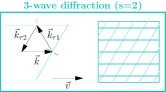
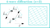
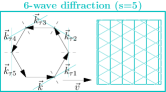
Figure 2:

This means that the VFEL is a self-phase-locking generator of radiation (phase-locking inside). When $N$ number of electron beams pass through electromagnetic crystals, the radiated power will increase in proportion to $N^{2}$ as a result of self-phase-locking of the beams due to two(three)-dimensional DFB formed in a VFEL resonator. When beams are generated, there is always a certain spread in the times when the produced electron bunches enter a VFEL resonator, which results from the instability of the current generation in a diode gap.

In the present paper it is shown that despite this spread in the entry times of the beams, a two(three)-dimensional feedback formed in a VFEL resonator gives rise to the self-phase-locking process . Equations are derived that describe the process of radiation generation by several electron bunches and enable studying the process of superradiation produced by the bunches, depending on the difference between the times of their entry into the resonator. It is also shown that similar processes of self-phase-locking, which lead to the power increase $W\sim N^{2}$ can also be observed when generation from electron bunches is excited in a system of several relativistic BWOs, whose corrugated waveguides form a single resonator by means of, e.g., slots (long bridge corrugated waveguides or diffraction grating) made in a cylinder along the axis of the waveguides.

2 Lasing equations for the system with a photonic crystal (diffraction grating) with changing parameters

In the general case the equations, which describe lasing process, follow from the Maxwell equations:

$$\textrm{rot}\vec{H}=\frac{1}{c}\frac{\partial\vec{D}}{\partial t}+\frac{4\pi}{c}\vec{j},\leavevmode\nobreak\ \textrm{rot}\vec{E}=-\frac{1}{c}\frac{\partial\vec{H}}{\partial t},$$ (1)

$$\textrm{div}\vec{D}=4\pi\rho,\leavevmode\nobreak\ \frac{\partial\rho}{\partial t}+\textrm{div}\vec{j}=0,$$

here $\vec{E}$ and $\vec{H}$ are the electric and magnetic fields, $\vec{j}$ and $\rho$ are the current and charge densities, the electromagnetic induction $D_{i}(\vec{r},t^{\prime})=\int\varepsilon_{il}(\vec{r},t-t^{\prime})E_{l}(\vec{r},t^{\prime})dt^{\prime}$ and, therefore, $D_{i}(\vec{r},\omega)=\varepsilon_{il}(\vec{r},\omega)E_{l}(\vec{r},\omega)$, the indices $i,l=1,2,3$ correspond to the axes $x,y,z$, respectively.

The current and charge densities are respectively defined as:

$$\vec{j}(\vec{r},t)=e\sum_{\alpha}\vec{v}_{\alpha}(t)\delta(\vec{r}-\vec{r}_{\alpha}(t)),\leavevmode\nobreak\ \rho(\vec{r},t)=e\sum_{\alpha}\delta(\vec{r}-\vec{r}_{\alpha}(t)),$$ (2)

where $e$ is the electron charge, $\vec{v}_{\alpha}$ is the velocity of the particle $\alpha$ ($\alpha$ numerates the beam particles),

$$\frac{d\vec{v}_{\alpha}}{dt}=\frac{e}{m\gamma_{\alpha}}\left\{\vec{E}(\vec{r}_{\alpha}(t),t)+\frac{1}{c}[\vec{v}_{\alpha}(t)\times\vec{H}(\vec{r}_{\alpha}(t),t)]-\frac{\vec{v}_{\alpha}}{c^{2}}(\vec{v}_{\alpha}(t)\vec{E}(\vec{r}_{\alpha}(t),t))\right\},$$ (3)

here $\gamma_{\alpha}=(1-\frac{v_{\alpha}^{2}}{c^{2}})^{-\frac{1}{2}}$ is the Lorentz-factor, $\vec{E}(\vec{r}_{\alpha}(t),t)$ ($\vec{H}(\vec{r}_{\alpha}(t),t)$) is the electric (magnetic) field at the point of location $\vec{r}_{\alpha}$ of particle $\alpha$.

It should be recalled that (3) can also be written as

$$\frac{d\vec{p}_{\alpha}}{dt}=m\frac{d\gamma_{\alpha}v_{\alpha}}{dt}={e}\left\{\vec{E}(\vec{r}_{\alpha}(t),t)+\frac{1}{c}[\vec{v}_{\alpha}(t)\times\vec{H}(\vec{r}_{\alpha}(t),t)]\right\},$$ (4)

where $p_{\alpha}$ is the particle momentum.

Let us recall here that the change in the particle energy through the its interaction with electromagnetic fields is described by the equation

$$mc^{2}\frac{d\gamma_{\alpha}}{dt}=e\vec{v}_{\alpha}\vec{E}(\vec{r}_{\alpha}(t),t).$$ (5)

Combining the equations in (1), we obtain:

$$-\Delta\vec{E}+\vec{\nabla}(\vec{\nabla}\vec{E})+\frac{1}{c^{2}}\frac{\partial^{2}\vec{D}}{\partial t^{2}}=-\frac{4\pi}{c^{2}}\frac{\partial\vec{j}}{\partial t}.$$ (6)

The dielectric permittivity tensor can be expressed as $\hat{\varepsilon}(\vec{r})=1+\hat{\chi}(\vec{r})$, where $\hat{\chi}(\vec{r})$ is the dielectric susceptibility. When $\hat{\chi}\ll 1$, (6) can be rewritten as:

$$\Delta\vec{E}(\vec{r},t)-\frac{1}{c^{2}}\frac{\partial^{2}}{\partial t^{2}}\int\hat{\varepsilon}(\vec{r},t-t^{\prime})\vec{E}(\vec{r},t^{\prime})dt^{\prime}=4\pi\left(\frac{1}{c^{2}}\frac{\partial\vec{j}(\vec{r},t)}{\partial t}+\vec{\nabla}\rho(\vec{r},t)\right).$$ (7)

When the grating is ideal $\hat{\chi}(\vec{r})=\sum_{\tau}\hat{\chi}_{\tau}(\vec{r})e^{i\vec{\tau}\vec{r}}$, where $\vec{\tau}$ is the reciprocal lattice vector.

Let the photonic crystal (diffraction grating) period be smoothly varied with distance, which is much greater then the diffraction grating (ptotonic crystal lattice) period. It is convenient in this case to present the susceptibility $\hat{\chi}(\vec{r})$ in the form, typical of the theory of X-ray diffraction in crystals with lattice distortion [6]:

$$\hat{\chi}(\vec{r})=\sum_{\tau}e^{i\Phi_{\tau}(\vec{r})}\hat{\chi}_{\tau}(\vec{r}),$$ (8)

where $\Phi_{\tau}(\vec{r})=\int\vec{\tau}(\vec{r}^{\,\prime})d\vec{l}^{\prime}$, $\vec{\tau}(\vec{r}^{\,\prime})$ is the reciprocal lattice vector in the vicinity of the point $\vec{r}^{\,\prime}$. In contrast to the theory of X-rays diffraction, in the case under consideration $\hat{\chi}_{\tau}$ can also depend on $\vec{r}$. Moreover, $\hat{\chi}_{\tau}$ depends on the volume of the lattice unit cell $\Omega$, which can be significantly varied for diffraction gratings (photonic crystals), as distinct from natural crystals. The volume of the unit cell $\Omega(\vec{r})$ depends on coordinate and, for example, for a cubic lattice it is determined as $\Omega(\vec{r})=\frac{1}{d_{1}(\vec{r})d_{2}(\vec{r})d_{3}(\vec{r})}$, where $d_{i}$ are the lattice periods. If $\hat{\chi}_{\tau}(\vec{r})$ does not depend on $\vec{r}$, the expression (8) converts to that usually used for X-rays in crystals with lattice distortion.

Recall here that for an ideal crystal without lattice distortions, the wave, which propagates in the crystal can be presented as a superposition of plane waves:

$$\vec{E}(\vec{r},t)=\sum_{\vec{\tau}=0}^{\infty}\vec{A}_{\vec{\tau}}e^{i(\vec{k}_{\tau}\vec{r}-\omega t)},$$ (9)

where $\vec{k}_{\tau}=\vec{k}+\vec{\tau}$.

Let us now use the fact that in the case under consideration the typical length for the change of the lattice parameters significantly exceeds the lattice period. Then the field inside the crystal with lattice distortion can be expressed similarly to (9), but with $\vec{A}_{\vec{\tau}}$ depending on $\vec{r}$ and $t$ and changing noticeably at the distances much greater than the lattice period.

Similarly, the wave vector should be considered as a slowly changing function of a coordinate.

According to the above, let us find the solution of (7) in the form:

$$\vec{E}(\vec{r},t)=\textrm{Re}\left\{\sum_{\vec{\tau}=0}^{\infty}\vec{A}_{\vec{\tau}}e^{i(\phi_{\tau}(\vec{r})-\omega t)}\right\},$$ (10)

where $\phi_{\tau}(\vec{r})=\int_{0}^{\vec{r}}k(\vec{r})d\vec{l}+\Phi_{\tau}(\vec{r})$, where $k(\vec{r})$ can be found as a solution of the dispersion equation in the vicinity of the point with the coordinate vector $\vec{r}$, integration is made over the quasiclassical trajectory, which describes motion of the wavepacket in the crystal with lattice distortion.

Now let us consider the case when all the waves participating in the diffraction process lie in a plane (coupled wave diffraction, multiple-wave diffraction), i.e., all the reciprocal lattice vectors $\vec{\tau}$ lie in one plane. Suppose the wave polarization vector is orthogonal to the plane of diffraction.

Let us rewrite (10) in the form

$$\vec{E}(\vec{r},t)=\vec{e}\,E(\vec{r},t)=\vec{e}\,\textrm{Re}\left\{{A}_{1}e^{i(\phi_{1}(\vec{r})-\omega t)}+{A}_{2}e^{i(\phi_{2}(\vec{r})-\omega t)}+...\right\},$$ (11)

where

$$\phi_{1}(\vec{r})=\int_{0}^{\vec{r}}\vec{k}_{1}(\vec{r}^{\,\prime})d\vec{l},$$ (12)

$$\phi_{2}(\vec{r})=\int_{0}^{\vec{r}}\vec{k}_{1}(\vec{r}^{\,\prime})d\vec{l}+\int_{0}^{\vec{r}}\vec{\tau}(\vec{r}^{\,\prime})d\vec{l}.$$ (13)

Then multiplying (7) by $\vec{e}$, one can get:

$$\Delta{E}(\vec{r},t)-\frac{1}{c^{2}}\frac{\partial^{2}}{\partial t^{2}}\int\hat{\varepsilon}(\vec{r},t-t^{\prime}){E}(\vec{r},t^{\prime})dt^{\prime}=4\pi\vec{e}\left(\frac{1}{c^{2}}\frac{\partial\vec{j}(\vec{r},t)}{\partial t}+\vec{\nabla}\rho(\vec{r},t)\right).$$ (14)

Applying the equality $\Delta{E}(\vec{r},t)=\vec{\nabla}(\vec{\nabla}E)$ and using (11), we obtain

$$\Delta(A_{1}e^{i(\phi_{1}(\vec{r})-\omega t)})=e^{i(\phi_{1}(\vec{r})-\omega t)}[2i\vec{\nabla}\phi_{1}\vec{\nabla}A_{1}+i\vec{\nabla}\vec{k}_{1}(\vec{r})A_{1}-k_{1}^{2}(\vec{r})A_{1}],$$ (15)

Therefore, substitution of the above expression into (14) gives the following system:

$$\frac{1}{2}e^{i(\phi_{1}(\vec{r})-\omega t)}\left[2i\vec{k}_{1}(\vec{r})\vec{\nabla}A_{1}+i\vec{\nabla}\vec{k}_{1}(\vec{r})A_{1}-k_{1}^{2}(\vec{r})A_{1}\right.$$

$$\left.+\frac{\omega^{2}}{c^{2}}\varepsilon_{0}(\omega,\vec{r})A_{1}+i\frac{1}{c^{2}}\frac{\partial\omega^{2}\varepsilon_{0}(\omega,\vec{r})}{\partial\omega}\frac{\partial A_{1}}{\partial t}+\frac{\omega^{2}}{c^{2}}\varepsilon_{-\tau}(\omega,\vec{r})A_{2}\right.$$

$$+\left.i\frac{1}{c^{2}}\frac{\partial\omega^{2}\varepsilon_{-\tau}(\omega,\vec{r})}{\partial\omega}\frac{\partial A_{2}}{\partial t}\right]$$

$$+\textrm{\leavevmode\nobreak\ conjugated\leavevmode\nobreak\ terms\leavevmode\nobreak\ }=4\pi\vec{e}\left(\frac{1}{c^{2}}\frac{\partial\vec{j}(\vec{r},t)}{\partial t}+\vec{\nabla}\rho(\vec{r},t)\right),$$

$$\frac{1}{2}e^{i(\phi_{2}(\vec{r})-\omega t)}[2i\vec{k}_{2}(\vec{r})\vec{\nabla}A_{2}+i\vec{\nabla}\vec{k}_{2}(\vec{r})A_{2}-k_{2}^{2}(\vec{r})A_{2}$$

$$+\frac{\omega^{2}}{c^{2}}\varepsilon_{0}(\omega,\vec{r})A_{2}+i\frac{1}{c^{2}}\frac{\partial\omega^{2}\varepsilon_{0}(\omega,\vec{r})}{\partial\omega}\frac{\partial A_{2}}{\partial t}+\frac{\omega^{2}}{c^{2}}\varepsilon_{\tau}(\omega,\vec{r})A_{1}$$

$$+i\frac{1}{c^{2}}\frac{\partial\omega^{2}\varepsilon_{\tau}(\omega,\vec{r})}{\partial\omega}\frac{\partial A_{1}}{\partial t}]$$

$$+\textrm{\leavevmode\nobreak\ conjugated\leavevmode\nobreak\ terms\leavevmode\nobreak\ }=4\pi\vec{e}\left(\frac{1}{c^{2}}\frac{\partial\vec{j}(\vec{r},t)}{\partial t}+\vec{\nabla}\rho(\vec{r},t)\right),$$ (16)

where vector $\vec{k}_{2}(\vec{r})=\vec{k}_{1}(\vec{r})+\vec{\tau}$, $\varepsilon_{0}(\omega,\vec{r})=1+{\chi}_{0}(\vec{r})$, here the notation ${\chi}_{0}(\vec{r})={\chi}_{\tau=0}(\vec{r})$ is used, $\varepsilon_{\tau}(\omega,\vec{r})={\chi}_{\tau}(\vec{r})$. Note here that for a numerical analysis of (16), if ${\chi}_{0}\ll 0$, it is convenient to take vector $\vec{k}_{1}(\vec{r})$ in the form $\vec{k}_{1}(\vec{r})=\vec{n}\sqrt{k^{2}+\frac{\omega^{2}}{c^{2}}\chi_{0}(\vec{r})}$.

Let us multiply the first equation by $e^{-i(\phi_{1}(\vec{r})-\omega t)}$ and the second by $e^{-i(\phi_{2}(\vec{r})-\omega t)}$. This procedure enables neglecting the conjugated terms, which appear fast oscillating (when averaging over the oscillation period they become zero).

Considering the right-hand side of (16), let us take into account that microscopic currents and densities are the sums of terms, containing delta-functions, therefore, the right-hand side can be rewritten as:

$$e^{-i(\phi_{1}(\vec{r})-\omega t)}4\pi\vec{e}\left(\frac{1}{c^{2}}\frac{\partial\vec{j}(\vec{r},t)}{\partial t}+\vec{\nabla}\rho(\vec{r},t)\right)$$ (17)

$$=-\frac{4\pi i\omega e}{c^{2}}\vec{e}\sum_{\alpha}\vec{v}_{\alpha}(t)\delta(\vec{r}-\vec{r}_{\alpha}(t))e^{-i(\phi_{1}(\vec{r})-\omega t)}\,\theta(t-t_{\alpha})\,\theta(T_{\alpha}-t).$$

Here $t_{\alpha}$ is the time of entrance of particle $\alpha$ to the resonator, $T_{\alpha}$ is the time of particle leaving the resonator, $\theta-$functions in (17) indicate that for the time moments preceding $t_{\alpha}$ and following $T_{\alpha}$, the particle ${\alpha}$ does not contribute to the process.

Upon averaging the system of equations over the oscillation period $\frac{2\pi}{\omega}$, we can write:

$$\left[2i\vec{k}_{1}(\vec{r})\vec{\nabla}A_{1}+i\vec{\nabla}\vec{k}_{1}(\vec{r})A_{1}-k_{1}^{2}(\vec{r})A_{1}+\frac{\omega^{2}}{c^{2}}\varepsilon_{0}(\omega,\vec{r})A_{1}\right.$$

$$\left.+i\frac{1}{c^{2}}\frac{\partial\omega^{2}\varepsilon_{0}(\omega,\vec{r})}{\partial\omega}\frac{\partial A_{1}}{\partial t}+\frac{\omega^{2}}{c^{2}}\varepsilon_{-\tau}(\omega,\vec{r})A_{2}+i\frac{1}{c^{2}}\frac{\partial\omega^{2}\varepsilon_{-\tau}(\omega,\vec{r})}{\partial\omega}\frac{\partial A_{2}}{\partial t}\right]$$ (18)

$$=-\frac{8\pi i\omega e}{c^{2}}\sum_{\alpha}\int^{t+\frac{2\pi}{\omega}}_{t}\vec{e}\,\vec{v}_{\alpha}(t^{\prime})\delta(\vec{r}-\vec{r}_{\alpha}(t^{\prime},t_{\alpha},\vec{r}_{\alpha 0})e^{-i\varphi_{1}[\vec{r}_{\alpha}(t^{\prime},t_{\alpha},\vec{r}_{\alpha\,0}),t^{\prime}]}\theta(t^{\prime}-t_{\alpha})\theta(t_{\alpha}-t^{\prime}),$$

where the phase $\varphi_{1}[\vec{r}_{\alpha}(t^{\prime},t_{\alpha},\vec{r}_{\alpha\,0}),t^{\prime}]=\phi_{1}(\vec{r}_{\alpha}(t^{\prime},t_{\alpha},\vec{r}_{\alpha\,0})-\omega t^{\prime}$.

$$\left[2i\vec{k}_{2}(\vec{r})\vec{\nabla}A_{2}+i\vec{\nabla}\vec{k}_{2}(\vec{r})A_{2}-k_{2}^{2}(\vec{r})A_{2}+\frac{\omega^{2}}{c^{2}}\varepsilon_{0}(\omega,\vec{r})A_{2}\right.$$

$$\left.+i\frac{1}{c^{2}}\frac{\partial\omega^{2}\varepsilon_{0}(\omega,\vec{r})}{\partial\omega}\frac{\partial A_{2}}{\partial t}+\frac{\omega^{2}}{c^{2}}\varepsilon_{\tau}(\omega,\vec{r})A_{1}+i\frac{1}{c^{2}}\frac{\partial\omega^{2}\varepsilon_{\tau}(\omega,\vec{r})}{\partial\omega}\frac{\partial A_{1}}{\partial t}\right]$$ (19)

$$=-\frac{8\pi i\omega e}{c^{2}}\sum_{\alpha}\int^{t+\frac{2\pi}{\omega}}_{t}\vec{e}\,\vec{v}_{\alpha}(t^{\prime})\delta(\vec{r}-\vec{r}_{\alpha}(t^{\prime},t_{\alpha},\vec{r}_{\alpha 0})e^{-i\varphi_{2}[\vec{r}_{\alpha}(t^{\prime},t_{\alpha},\vec{r}_{\alpha\,0}),t^{\prime}]}\theta(t^{\prime}-t_{\alpha})\theta(t_{\alpha}-t^{\prime}),$$

where the phase $\varphi_{2}[\vec{r}_{\alpha}(t^{\prime},t_{\alpha},\vec{r}_{\alpha\,0}),t^{\prime}]=\phi_{2}(\vec{r}_{\alpha}(t^{\prime},t_{\alpha},\vec{r}_{\alpha\,0})-\omega t^{\prime}$ and $\varepsilon_{0}=1+\chi_{0}$, $\varepsilon_{\tau}=\chi_{\tau}$.

When several ($N$ number) electron beams move through a spatially periodic medium, the sum $\sum_{\alpha}$ over the particles can be represented as a sum of contributions coming from individual electron beams to the total current:

$$\sum_{\alpha}=\sum_{\alpha_{1}}+\sum_{\alpha_{2}}+...\sum_{\alpha\,N},$$

where $N$ is the number of electron beams.

Using the definitions of $\phi_{m}$ (see (12), (13) we can obtain the following relationship for the phases $\varphi_{m}$:

$$\frac{d\varphi_{m}}{dt}=\vec{k}_{m}(\vec{r}_{\alpha}(t,t_{\alpha},r_{\alpha\,0}))\vec{v}_{\alpha}(t)-\omega$$ (20)

and

$$\frac{d^{2}\varphi_{m}}{dt^{2}}=\vec{v}_{\alpha}(t)\frac{d\vec{k}_{m}(r_{\alpha}(t))}{dt}+\vec{k}_{m}(r_{\alpha}(t))\frac{d\vec{v}_{\alpha}}{dt}.$$ (21)

Equations (3)–(5), describing particle motion in electromagnetic fields, and equations (2)–(2) for the fields are written using slowly changing amplitudes $A$ and phases $\varphi_{m}=\phi_{m}-\omega t$. They give a closed, nonlinear set of equations that defines the amplitude $A_{m}$ and phases $\varphi_{m}$ (as well as the change in the energy of particles interacting with the fields) and can be numerically analyzed using, say, the large-particle method.

Because of random distribution of particles in the bunches incident on a resonator (electromagnetic, photonic crystal), the times $t_{\alpha}$ of particle entry into the resonator as well as the distribution of the entry point coordinates $\vec{r}_{s}$ of the bunch particles over the entire surface of the resonator are random. Each bunch also has a certain distribution of initial velocities $\vec{v}_{\alpha}^{(0)}$. This enables one to average (2) and (2) over the distribution of the quantities $t_{\alpha}$$\vec{r}_{s}$, and $\vec{v}_{\alpha}^{(0)}$. Such averaging can be made by generalizing the averaging method developed for the case of one-dimensional generators like TWT, BWO, FEL to the case of a non-one-dimensional distributed feedback (DFB) The equations obtained as a result of such averaging in a stationary case when one beam moves in a VFEL resonator are given in [6].

We shall further consider self-phase-locking arising when photons are emitted by several electron beams in a spatially periodic VFEL resonator in the case of quasi-Cherenkov (diffraction) spontaneous radiation mechanism (recall here that this radiation mechanism underlies the operation of conventional one-dimensional TWTs and BWOs).

For better understanding, let us suppose now that a strong magnetic field is applied for beam guiding through the generation area. Electron beams move along the direction of this field. Let us choose the direction of beam motion as the $z$-axis. We shall also consider the case when the period of the resonator’s diffraction grating changes along the direction of the $z$-axis. In this case, equations (2) and (2) can be presented in the form:

$$\left[2i\vec{k}_{1}(\vec{r})\vec{\nabla}A_{1}+i\vec{\nabla}\vec{k}_{1}(\vec{r})A_{1}-k_{1}^{2}(\vec{r})A_{1}\frac{\omega^{2}}{c^{2}}\varepsilon_{0}(\omega,\vec{r})A_{1}\right.$$

$$\left.+i\frac{1}{c^{2}}\frac{\partial\omega^{2}\varepsilon_{0}(\omega,\vec{r})}{\partial\omega}\frac{\partial A_{1}}{\partial t}+\frac{\omega^{2}}{c^{2}}\varepsilon_{-\tau}(\omega,\vec{r})A_{2}+i\frac{1}{c^{2}}\frac{\partial\omega^{2}\varepsilon_{-\tau}(\omega,\vec{r})}{\partial\omega}\frac{\partial A_{2}}{\partial t}\right]$$

$$=-\frac{8\pi i\omega e\vartheta_{1}}{c^{2}}g_{1}(r_{\perp},z,t),$$ (22)

where

$$g_{1}(r_{\perp},z,t) = \sum_{N}\langle\langle\int^{t+\frac{2\pi}{\omega}}_{t}\sum_{\alpha_{N}}u_{\alpha_{N}}(t)\delta(r_{\perp}-r_{\alpha_{N}\perp})\delta(z-z_{\alpha_{N}}(t^{\prime},t_{\alpha_{N}},u_{\alpha_{N}}^{(0)}))$$

$$\times e^{-i\vec{k}_{\perp}\vec{r}_{\alpha_{N}\perp}}e^{-i[\phi_{1}(z_{\alpha}(t^{\prime},t_{\alpha_{N}},u_{\alpha_{N}}^{(0)}))-\omega t^{\prime}]}\theta(t^{\prime}-t_{\alpha})\theta(T_{\alpha-t^{\prime}})\rangle\rangle dt^{\prime},$$

$$\left[2i\vec{k}_{2}(\vec{r})\vec{\nabla}A_{2}+i\vec{\nabla}\vec{k}_{2}(\vec{r})A_{2}-k_{2}^{2}(\vec{r})A_{2}+\frac{\omega^{2}}{c^{2}}\varepsilon_{0}(\omega,\vec{r})A_{2}\right.$$

$$\left.+i\frac{1}{c^{2}}\frac{\partial\omega^{2}\varepsilon_{0}(\omega,\vec{r})}{\partial\omega}\frac{\partial A_{2}}{\partial t}+\frac{\omega^{2}}{c^{2}}\varepsilon_{\tau}(\omega,\vec{r})A_{1}+i\frac{1}{c^{2}}\frac{\partial\omega^{2}\varepsilon_{\tau}(\omega,\vec{r})}{\partial\omega}\frac{\partial A_{1}}{\partial t}\right]$$

$$=-\frac{8\pi i\omega e\vartheta_{2}}{c^{2}}g_{2}(r_{\perp},z,t),$$ (23)

where

$$g_{2}(r_{\perp},z,t) = \sum_{N}\langle\langle\int^{t+\frac{2\pi}{\omega}}_{t}\sum_{\alpha_{N}}u_{\alpha_{N}}(t)\delta(r_{\perp}-r_{\alpha_{N}\perp})\delta(z-z_{\alpha_{N}}(t^{\prime},t_{\alpha_{N}},u_{\alpha_{N}}^{(0)}))$$

$$\times e^{-i\vec{k}_{\perp}\vec{r}_{\alpha_{N}\perp}}e^{-i[\phi_{2}(z_{\alpha}(t^{\prime},t_{\alpha_{N}},u_{\alpha_{N}}^{(0)}))-\omega t^{\prime}]}\theta(t^{\prime}-t_{\alpha})\theta(T_{\alpha-t^{\prime}})\rangle\rangle dt^{\prime}.$$

Here $\phi_{1}(z_{\alpha}(t^{\prime},t_{\alpha_{N}},u_{\alpha_{N}}^{(0)}))=\int_{0}^{z_{\alpha}(t^{\prime},t_{\alpha_{N}},u_{\alpha_{N}}^{(0)}))}k_{1z}(z^{\prime})dz^{\prime}$ and $\phi_{2}(z_{\alpha}(t^{\prime},t_{\alpha_{N}},u_{\alpha_{N}}^{(0)}))=\int_{0}^{z_{\alpha}(t^{\prime},t_{\alpha_{N}},u_{\alpha_{N}}^{(0)}))}k_{2z}(z^{\prime})dz^{\prime}$. If the period of the diffraction grating is constant along the $z$-axis, then $\phi_{1}=k_{1}z_{\alpha}(t^{\prime},t_{\alpha_{N}},u_{\alpha_{N}}^{(0)})$. The sign $\langle\langle...\rangle\rangle$ means averaging over the distribution of beam particles over the transverse coordinate of the entry points, the entry time, and over the velocity distribution of the beams entering the resonator;

$$\vartheta_{m}=\sqrt{1-\frac{\omega^{2}}{\beta^{2}k_{m}^{2}c^{2}}},\quad\beta^{2}=1-\frac{1}{\gamma^{2}},\quad\vec{k}_{1}=\vec{k}_{\tau=0},\quad\vec{k}_{2}=\vec{k}_{1}+\vec{\tau}.$$

Let $\rho(\vec{r}_{\perp})$ denote the particle density in the plane transverse relative to the particle velocity and $\dot{n}$ denote the number of particles traversing the inner surface of the resonator per unit time. We also make use of the fact that

$$\delta(z-z_{\alpha_{N}}(t^{\prime},t_{\alpha_{N}},u_{\alpha_{N}}^{(0)}))=\delta(t^{\prime}-\tau(z,t_{\alpha_{N}},u_{\alpha_{N}}^{(0)}))/\left|\frac{\partial z_{\alpha_{N}}(t^{\prime},t_{\alpha_{N}},u_{\alpha_{N}}^{(0)})}{\partial t^{\prime}}\right|,$$

where

$$\tau(z,t_{\alpha_{N}},u_{\alpha_{N}}^{(0)})=t_{\alpha_{N}}+\int_{0}^{z}\frac{dz^{\prime}}{u_{N}(z^{\prime},t_{\alpha_{N}}u_{\alpha_{N}}^{(0)})}.$$

Here $\tau$ is the time required for the particle entering the interaction area $z=0$ at time $t_{\alpha}$ at initial speed $u_{\alpha_{N}}^{(0)}$ to reach the point $z$ and $u_{N}(z,t_{\alpha_{N}},u_{\alpha_{N}}^{(0)})$ is the speed at point $z$ for the particle whose initial speed at $z=0$ and time $t_{\alpha_{N}}$ equaled $u_{\alpha_{N}}^{(0)}$, while $\frac{\partial z_{\alpha_{N}}(t^{\prime},t_{\alpha_{N}},u_{\alpha_{N}}^{(0)})}{\partial t^{\prime}}$ is the particle speed at time $t$ if at $z=0$ and $t_{\alpha_{N}}$ its speed was $u_{\alpha_{N}}^{(0)}$. Obviously, for the expression to be finite, this speed should not vanish; otherwise, such transformation of the $\delta$-function becomes invalid (this is possible, for example, in the case when the beam’s current exceeds the so-called limiting current and the virtual cathode is formed).

We shall further assume that the particles are not retarded significantly during the interaction and write the quantity in the denominator of $\frac{\partial z_{\alpha_{N}}}{\partial t}=u_{\alpha_{N}}^{(0)}$. As a result, we have $\frac{\dot{n}}{u_{\alpha}}=\rho_{z}(t_{\alpha})$, where $\rho_{z}(t_{\alpha})$ is the beam’s time-dependent density distribution along the $z$-axis.

Let us also suppose that the duration of the bunches injected into the resonator is larger than the period $\frac{2\pi}{\omega}$ of excited oscillations of the electromagnetic wave. Taking into account the relationship for $\tau=t_{\alpha_{N}}+\frac{z}{u_{\alpha}}$, which follows in this case from the $\delta$-function, the distribution density $\rho_{z}(t^{\prime}_{\alpha})$ in this case can be removed from the sign of integration over the entry time $t_{\alpha_{N}}$ at point $t^{\prime}-\frac{z}{u_{\alpha}}$, and so we have

$$\rho_{z}(t_{\alpha})=\rho_{z}(t^{\prime}-\frac{z}{u_{\alpha}}).$$

In a real situation, the distribution of the beam’s longitudinal velocity is much less than the average longitudinal velocity of the bunch, so we can remove the density $\rho_{z}$ from the sign of integration describing averaging over the velocity distribution. However, analyzing the phase dependence on the velocity distribution of particles in a bunch, one should bear in mind that the velocity distribution can appreciably affect the phase.

As a result, we can obtain the following expression for $g_{n}$:

$$g_{n}(r_{\perp},z,t) = \sum_{N}e^{-i\vec{k}_{\perp}\vec{r}_{\perp}}\rho_{N}(r_{\perp},z-u_{N}t)$$ (24)

$$\times u_{N}\int_{t-\frac{z}{u_{N}}}^{t-\frac{z}{u_{N}}+\frac{2\pi}{\omega}}e^{-i[\phi_{n}(z(\tau,t_{0},u^{(0)}))-\omega\tau(t_{\alpha},u^{(0)})]}f(u_{N}^{(0)})du_{N}^{(0)}dt_{0}.$$

Here $dt_{0}$ means integration over the initial times, $f(u^{(0)}_{N})$ is the velocity distribution function in bunch $N$, and $u_{N}$ is the average velocity of the $N$-th bunch; the right-hand part of equation differs from zero at times $t>0$ from the initial moment defined as the instant of time when the first particle of the first bunch enters the resonator.

The derived set of equations enables describing the process of radiation from several beams in a spatially periodic system (photonic crystal), including the case when the beams move opposite to one another. The geometry when the beams move opposite to one another can be used for beam diagnosing in the bunch-bunch collision region in colliding-beam storage rings. For short bunches, this set of equations describes the phenomenon of super-radiance produced when several bunches of relativistic particles pass through a VFEL resonator. Particularly, it is possible to investigate radiation as a function of the difference between the times of electron bunches entry into the photonic crystal and as a function of the transverse distance between the bunches moving in the electromagnetic (photonic) crystal.

According to the equations derived here, the electromagnetic field induced in the crystal by different beams does not contain random phases $r_{\alpha_{N}}$ and $t_{\alpha}$ any longer, and the total field, as a result, is a coherent sum of the induced fields, which means that the radiation power increases as ${W\sim E^{2}=(\sum_{N}E_{n})^{2}\simeq N^{2}E_{1}}$. It should be noted that when the parameters $\chi_{\tau}$ grow, $|\chi_{\tau}|\geq 1$, the plane-wave expansion of the solution to Maxwell’equations, which is used in the dynamical diffraction of waves in crystals, requires that for accurate description of the radiation generation process a larger number of waves should be considered. However, in this case one can expand the electromagnetic field into the analogue of the Wannier functions, which are used for describing the band structure of electrons in crystals in the case of tight binding.

Let us consider the following example. Let a spatially periodic resonator be formed by axially corrugated cylindrical waveguides. we shall choose the direction of the waguides’ axis as the $z$-axis. Coupled through the slots in their walls (long bridge corrugated waveguides or diffraction grating), the waveguide form a single spatially periodic electrodynamical system. In the general case, we have a 2D periodic system in the ($x,y$) plane, orthogonal to the $z$-axis. The beams move along the $z$-axis. Depending on the position of the cylinders in the transverse plane, square gratings or more complicated structures can be formed, e.g the cylinders can be arranged in a circle (as it occurs in the magnetron).

To describe generation in this system, it is convenient start with the expansion Maxwell’s equations in terms of the eigenfuctions $\vec{Y}_{n}(\vec{r}_{\perp})$ of this transverse grating (see a similar approach used for describing the motion of fast electrons in crystals in channeling regime (mode)) [7]. In this case the eigenfunction $\vec{Y}_{n}(\vec{r}_{\perp})$ is a sum of the localized Wannier functions $W_{n}$

$$\vec{Y}_{n\vec{\kappa}}(\vec{r})=\sum_{m}W_{n}(\vec{r}_{\perp}-\vec{R}_{\perp m})e^{i\vec{\kappa}\vec{R}_{\perp m}},$$

where $\vec{\kappa}$ is the reduced wave vector, $n$ is the set of indices defining stationary wave functions , e.g., the wave function used for the formation of the structures periodic in the transverse plane, and $\vec{R}_{m}$ is the coordinate of the centre of the elementary cell $m$ of the structure periodic in the transverse plane.

As a result, for the analysis of generation of radiation we obtain one dimensional along the $z$-axis equations, where the excitation current is the total current $I$ produced by the beams moving in the system. Let us average the current $I$ over the electron entry times, the distribution of the initial velocities, and the distribution of electrons in the transverse plane (which in this case have the peaks in the regions where the electrons from each beam producing the current $I$ move).

As a result we obtain the equations similar in form to those used for the analysis of the generation process induced by one beam moving in a waveguide that is spatially periodic along the $z$-axis axis (formed by , e.g., a corrugated waveguide of a relativistic BWO.) Hence, we can conclude that the considered system, excited by several beams, generates common coherent radiation. Now, let us give a more detailed consideration of the case when the resonator is formed by the two elements of the grating.

When the resonator period is formed by corrugation of the waveguide surface, we obtain a system consisting of two corrugated waveguides coupled through, say, a slot. For the BWO in the stationary case when two stationary electron beams move through circular waveguides, this system was analyzed neglecting the influence of the wave moving in the same direction [8]. Using numerical analysis, the authors of [8] showed that at certain parameters, a single-frequency oscillation mode is stet in the system, i.e., in fact, coherent summation of the amplitudes of the fields induced by two separate beams is possible. As follows from the above analysis, such coherent summation is also possible in the case non-stationary excitation of the system by two pulses of electron beams.

Note here that the equations derived in this paper enable taking account of the influence of a coherent wave on the generation process in a system of several BWOs. Moreover, according to [6], just in the range of parameters where the amplitudes of the incident and diffracted waves are comparable, in a two-three dimensional periodic system the increment of radiative instability increases sharply and the threshold for the generation start drops dramatically.

When applied to this case, general equations for describing the excitation of two relativistic BWOs by two pulses of electron beams can be written in the form:

Neglecting dispersion in considering the generation process in a system of two BWOs with a constant grating period (corrugation period), one can write these equations in the form:

$$\left\{\begin{array}[]{c}2ik_{1z}\frac{\partial A^{a}_{1}}{\partial z}+2i\frac{\omega}{c^{2}}\frac{\partial A^{a}_{1}}{\partial t}+\left[\frac{\omega^{2}}{c^{2}}\varepsilon_{0}-k^{2}_{mn}-k^{2}_{1z}\right]A_{1}^{a}\\ +\frac{\omega^{2}}{c^{2}}\varepsilon_{\tau}A_{2}^{a}+\frac{\omega^{2}}{c^{2}}\chi_{ab}^{1}A^{b}_{1}+\frac{\omega^{2}}{c^{2}}\chi^{2}_{ab}A^{b}_{2}=\vec{Y}_{mn}\vec{j}_{1},\\ \\ 2ik_{2z}\frac{\partial A^{a}_{2}}{\partial z}+2i\frac{\omega}{c^{2}}\frac{\partial A^{a}_{2}}{\partial t}+\left[\frac{\omega^{2}}{c^{2}}\varepsilon_{0}-k^{2}_{mn}-k^{2}_{2z}\right]A_{2}^{a}\\ +\frac{\omega^{2}}{c^{2}}\varepsilon_{\tau}A_{2}^{a}+\frac{\omega^{2}}{c^{2}}\chi_{ab}^{1}A^{b}_{1}+\frac{\omega^{2}}{c^{2}}\chi^{2}_{ab}A^{b}_{2}=\vec{Y}_{mn}\vec{j}_{1\tau},\end{array}\right.$$ (30)

$$\left\{\begin{array}[]{c}2ik_{1z}\frac{\partial A^{b}_{1}}{\partial z}+2i\frac{\omega}{c^{2}}\frac{\partial A^{b}_{1}}{\partial t}+\left[\frac{\omega^{2}}{c^{2}}\varepsilon_{0}-k^{2}_{mn}-k^{2}_{1z}\right]A_{1}^{b}\\ +\frac{\omega^{2}}{c^{2}}\varepsilon_{\tau}A_{2}^{b}+\frac{\omega^{2}}{c^{2}}\chi_{ab}^{1}A^{b}_{1}+\frac{\omega^{2}}{c^{2}}\chi^{2}_{ab}A^{b}_{2}=\vec{Y}_{mn}\vec{j}_{2},\\ \\ 2ik_{2z}\frac{\partial A^{b}_{2}}{\partial z}+2i\frac{\omega}{c^{2}}\frac{\partial A^{b}_{2}}{\partial t}+\left[\frac{\omega^{2}}{c^{2}}\varepsilon_{0}-k^{2}_{mn}-k^{2}_{2z}\right]A_{2}^{b}\\ +\frac{\omega^{2}}{c^{2}}\varepsilon_{\tau}A_{2}^{b}+\frac{\omega^{2}}{c^{2}}\chi_{ab}^{1}A^{b}_{1}+\frac{\omega^{2}}{c^{2}}\chi^{2}_{ab}A^{b}_{2}=\vec{Y}_{mn}\vec{j}_{2\tau},\end{array}\right.$$ (36)

We have for the BWO mode

$$A_{1}^{a(b)}(z=0)=0,\qquad A_{2}^{a(b)}(z=L)=0,$$

where $L$ is the resonator length.

For the case when more than two waveguides are involved, say, $N$ number - $N$ number of pairs of equation sets are required, instead of the two sets given above, and the terms describing the waves produced by other waveguides that are similar to $\chi_{ab}^{1}A_{1}^{b}$ and $\chi_{ab}^{2}A_{2}^{b}$ in (30), (36) should be added to each pair of equations.

It is worth noting that in a real case of arbitrary $\chi_{\tau}$, the coefficients appearing in these equations should be considered as phenomenological coefficients determined from the experiment on the passage of an electromagnetic wave through such structures.

The derived system of equations enables describing the process of generation excited by the combined pulses of electron bunches in a periodic system of coupled periodic waveguides (artificial electromagnetic crystal, VFEL resonator), which forms self-phase-locking of coherent oscillations. The derived set of equations enabled studying the dependence of the radiation power on the difference between the times of the bunches’entry into the resonator of such a periodic system. This equation set is applicable to describing radiation produced by bunches with various duration, and consequently in the case of short bunches it allows one to describe the phenomenon of superradiation and phase-locking in the system of several relativistic BWOs coupled into the grating.

3 Conclusion

The above analysis shows that when a spatially periodic system of a VFEL resonator is excited by several ($N$) pulsed electron beams that enter the resonator at different times, the two-(three)-dimensional distributed feedback, formed in the resonator, gives rise to self-phase-locking of the radiation process and coherent collective oscillations, which result into a square in $N$ increase of the radiation power $W$ with growing number of beams: $W\sim N^{2}$. Such self-phase locking occurring in a VFEL resonator makes it possible for us to consider the VFEL as the self-phase-locking system. Using this equation set, one can describe generation of generation by several beams in different modes: as superradiation from several electron beams and as radiation from long beams. These equations also make it possible to study the process of generation of superadiation as a function of the difference between the times of bunches’ entry into the resonator.

References

• [1] Benford J., Swegle J.A., Schamilogly E. High power microwaves, Taylor and Francis, 2007, 531 p.
• [2] Clayborne D. Taylor, D. V. Giri, High Power Microwave Systems and Effects, Taylor and Francis Group, 1994.
• [3] W. Woo et al, J.Appl. Phys. 65, 2 (1989) 0021–8979/89/020861-06.
• [4] C.B. Wharton et al,Proc. of the 8th Int. Conf. on High-Energy Power Particle Beams (BEAMS’90), Novosibirsk, USSR, 1990, pp. 1229–1240.
• [5] A.A. Elchaninov et al, Zh. Tekh. Fiziki 81, 1 (2011) pp. 125–130.
• [6] V.G. Baryshevsky, LANL e-print arXiv:1211.4769[physics.optics].
• [7] V.G. Baryshevsky High-Energy Nuclear Optics of Polarized Particles, World Scientific, Singapore, 2012.
• [8] V.A. Balakirev, A.O. Ostrovsky, Yu. V. Tkach, Pis’ma Zh. Tekh. Fiziki 16, 19 (1990) pp. 8–12.