Confinement from Correlation Functions
Abstract
We compute the Polyakov loop potential in Yang–Mills theory from the fully dressed primitively divergent correlation functions only. This is done in a variety of functional approaches ranging from functional renormalisation group equations over Dyson–Schwinger equations to two-particle irreducible functionals. We present a confinement criterion that links the infrared behaviour of propagators and vertices to the Polyakov loop expectation value. The present work extends the works of Braun:2007bx ; Marhauser:2008fz ; Braun:2010cy to general functional methods and sharpens the confinement criterion presented there. The computations are based on the thermal correlation functions in the Landau gauge calculated in Fister:2011uw ; Fister:2011um ; Fister:Diss .
pacs:
12.38.Aw,11.10.Wx,11.15.TkI Introduction
In recent years much progress has been made in our understanding of the strongly-correlated low energy regime of QCD in terms of gauge-fixed correlation functions, for reviews see e.g. Alkofer:2000wg ; Roberts:2000aa ; Fischer:2006ub ; Fischer:2008uz ; Binosi:2009qm ; Pawlowski:2010ht ; Maas:2011se ; vonSmekal:2012vx . This progress is tightly linked to the advancement in our understanding of the basic phenomena of low energy QCD, strong chiral symmetry breaking and confinement. While chiral symmetry breaking allows for a simple description in terms of the related order parameter, the chiral condensate, and its effective potential, our understanding of the confinement-deconfinement phase transition and the mechanism behind is still less developed.
For static quarks with infinite masses, confinement can be thought of in terms of the free energy of a single quark . Removing the antiquark to infinity in a colourless system with a quark-antiquark pair requires an infinite amount of energy in a confined system. The corresponding free energy difference can be related to the free energy of a single quark. Indeed, the gauge field part of such an operator is the Polyakov loop ,
| (1) |
the trace in the fundamental representation of of the closed Wilson line in time direction. Here, denotes path ordering, is the gauge field and the inverse temperature . The related quark current comprises the worldline of a static quark. The free energy of such a state is proportional to the expectation value of ,
| (2) |
Hence, is an order parameter for confinement: it is strictly zero in the confined phase but non-zero in the deconfined phase. This links the confinement-deconfinement phase transition in the Yang–Mills system to the order-disorder phase transition of center symmetry in : Under center transformations the Polyakov loop transforms with in the fundamental representation. We conclude that in the center-symmetric, confining phase we have , while in the center-broken, deconfined phase we have .
In Braun:2007bx ; Marhauser:2008fz it has been shown that also for constant fields is an order parameter for static quark confinement. Note that the expectation value relates to the eigenvalues of with and is gauge-invariant and gauge-independent.
The order parameter has the advantageous property that its full effective potential can be computed straightforwardly with functional continuum methods. Within the functional renormalisation group (FRG) approach it has been shown Braun:2007bx ; Marhauser:2008fz ; Braun:2009gm , that the computation of has a closed representation in terms of the full propagators of gluon, ghosts (and quarks) in constant -backgrounds. This link of the propagators to the Polyakov loop potential also allowed to put forward a confinement criterion for the infrared behaviour of the ghost and gluon propagators Braun:2007bx .
As similar link of confinement to the infrared behaviour of (gauge-fixed) correlation functions has been put forward more recently with dual order parameters, Gattringer:2006ci ; Synatschke:2007bz ; Bilgici:2008qy ; Fischer:2009wc ; Fischer:2009gk ; Braun:2009gm ; Fischer:2011mz ; Fischer:2012vc ; Hopfer:2012qr . The latter class of order parameters is directly sensitive to spectral properties of the Dirac operator and hence is tightly linked to quark correlation functions. The former one, , is directly sensitive to the gluon and ghost correlation functions as well as to the quarks. Nonetheless, there is a close relation between the two classes of order parameters, which has been discussed in Braun:2009gm for fully dynamical two-flavour QCD at finite temperature. There it has been shown that the two order parameters concur for the case of the dual density or dual pressure.
By now and the effective Polyakov loop potential has been computed in Yang–Mills theory in the Landau gauge Braun:2007bx ; Braun:2010cy ; Eichhorn:2011gc , the Polyakov gauge Marhauser:2008fz and in the Coulomb gauge Reinhardt:2012qe . A comparison of in different gauges has been made in Marhauser:2008fz which confirms the formal results of gauge independence. More recently, there have been also first computations of the Polyakov loop potential in Yang-Mills theory on the lattice, see Diakonov:2012dx ; Greensite:2012dy . In Braun:2009gm the Yang–Mills studies have been extended to fully dynamical two-flavour QCD. In Fukushima:2012qa ; Kashiwa:2012td the Polyakov loop potential is used in an effective model approach to QCD with interesting applications to thermodynamic observables.
For a quantitative computation of the Polyakov loop potential, the temperature dependence of the order parameter and in particular the critical temperature a good grip on the thermal ghost and gluon propagtors is required. In Landau gauge they have been computed on the lattice, Cucchieri:2007ta ; Fischer:2010fx ; Maas:2011ez ; Bornyakov:2011jm ; Cucchieri:2011di ; Maas:2011se ; Aouane:2011fv ; Aouane:2012bk , and in the continuum, Fister:2011uw ; Fister:2011um ; Fister:Diss with FRG-methods, extending previous studies in extreme temperature limits in the Dyson–Schwinger framework Maas:2004se ; Gruter:2004bb ; Maas:2005hs ; Cucchieri:2007ta .
In the present work we compute the Polyakov loop effective potential in the background field formalism Abbott:1980hw in Landau–deWitt gauge within different functional approaches. In Section II we derive representations for the Polyakov loop potential within the FRG-approach, Dyson-Schwinger equations (DSEs) and the two-particle irreducible (2PI-) effective action. In Section III we extend and sharpen the confinement criterion of Braun:2007bx in terms of the propagators: Infrared suppression of gluons but non-suppression of ghosts suffices to confine static quarks. In Section IV the criterion is applied to general Yang–Mills-matter systems. In Section V the Polyakov loop potential is computed in Yang–Mills theory on the basis of the finite temperature propagators computed within the FRG in Fister:2011uw ; Fister:2011um ; Fister:Diss . The results for the different functional methods are in quantitative agreement in the confinement-deconfinement regime.
II Polyakov Loop Potential from Functional Methods
In this section we discuss different representations of the Polyakov loop potential derived from the FRG, DSEs and 2PI-functionals. The Polyakov loop potential is simply the free energy, or one-particle irreducible (1PI) effective action , evaluated on constant backgrounds .
II.1 Polyakov Loop Potential
Most functional approaches are based on closed expressions for the effective action or derivatives thereof in terms of full correlation functions. Hence, the knowledge of the latter in constant -backgrounds allows us to compute the Polyakov loop potential . In turn, confinement requires the Polyakov loop potential to have minima at the confining values for . In these are the center-symmetric points. This restricts the infrared behaviour of the correlation functions computed in the constant -background.
Gauge covariance of the correlation functions and gauge invariance of the effective action and, hence, the effective potential is achieved within the background field approach Abbott:1980hw . We split the gauge field in a background and fluctuations about the background, . This split allows us to define background field-dependent gauges that transform covariantly under gauge transformations of both the background and the full gauge field,
| (3) |
and . As a consequence all correlation functions transform covariantly under combined gauge transformations of and . Hence, the effective action is invariant under combined gauge transformations. However, due to the gauge (3) it now depends on the full gauge field and the background field separately, , where are the Faddeev-Popov ghosts. The path integral representation is in terms of field-multiplet and their expectation values ,
| (4) |
The classical action is given by
| (5) | |||||
where is the field strength tensor, the gauge fixing parameter and the abbreviation . If we now identify the background with the physical background , the expectation value of the field, we arrive at a gauge invariant effective action
| (6) |
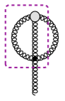
The Polyakov loop potential is given by (6) evaluated on a constant -background, ,
| (7) |
where is the three-dimensional spatial volume. The Polyakov loop, (1), is then evaluated at the minimum . It has been proven in Braun:2007bx and Marhauser:2008fz that (1) evaluated on the minimum of (7) is an order parameter such as .
Functional equations for the effective action can be derived from the FRG, DSEs and 2PI equations. All those equations depend on the correlation functions of fluctuation fields only, schematically given by
| (8) |
where we have suppressed the ghosts and the internal and Lorentz indices. In Braun:2007bx we have argued that the correlation functions in the background Landau gauge, , are directly related to those in Landau gauge, . This allows us to use the latter correlation functions within the computation of the effective potential. Here, we recall the argument given in Braun:2007bx for the ghost and gluon two-point functions, , which straightforwardly extends to higher correlation functions:
Gauge covariance of the fluctuation field correlation functions which constrains the difference between and . At vanishing temperature the gluon two-point function in Landau gauge splits into four-dimensionally transversal and longitudinal parts with the projection operators
| (9) |
Hence, the gluon propagator is transversal for all cut-off scales even though the longitudinal part of the inverse gluon propagator, receives finite corrections as well.
At non-vanishing temperature we have to take into account chromomagnetic and chromoelectric modes via the respective projection operators and ,
| (10) |
where is the four-dimensional transversal projection operator, see (9). The parameterisation of the gluon and ghost two-point functions in Landau gauge, i.e. the chromoelectric/chromomagnetic gluon and the ghost , is then given by, Fister:2011uw ; Fister:2011um ; Fister:Diss ,
| (11) |
where the identity in colour space is suppressed and the wave function renormalisations are functions of and separately. We now parameterise the background field correlation functions in terms of the Landau gauge correlation functions in (11) evaluated at covariant momenta. For the gluon this gives
| (12) | |||||
with non-singular , and where the arguments with respect to the covariant momentum of the projection operators onto the longitudinal and transversal spaces , respectively, and of have been omitted for clarity. Note that the projection operators do not commute with for general gauge fields. They do, however, for constant gauge fields . The -term can not be obtained alone from the Landau-gauge propagator, but is also related to higher Green functions. However, it does not play a rle for our purpose.
In the computations below we approximate the full inverse gluon propagators by the first line in (12). Similarly the inverse ghost propagator is approximated for constant temporal background as
| (13) |
For these backgrounds no -term as introduced in (12) is present. Note also that a mass term is kinematically forbidden for the ghost. Hence it can only contribute for momenta larger than zero. As it is subject to the standard thermal decay we neglect it as sub-leading.
II.2 Thermal Corrections and Critical Scaling
Here we discuss in detail the impact of the neglected thermal corrections . They play a crucial rle for the correct critical scaling and the value of in the -case but is sub-leading in the case. This section might be skipped in a first reading as the following results can be understood without it.
We know that vanishes at or . Moreover, the first two terms on the rhs in (12) parameterise all terms in that only depend on the covariant operator . At finite temperature, however, the Polyakov loop is a further invariant, i.e. the Polyakov line, , cf. (1), transforms covariantly under gauge transformations. These terms are particularly important for the chromoelectric component of the gluon two-point function (12) as they depend on . Moreover, these terms are not covered by the Landau gauge term in (12) as the related variable is not present for . In addition, has the standard thermal decay for large momenta . Hence we shall only discuss it for the low momentum regime, that is . Note also that (1) is invariant under the periodic gauge transformation with
| (14) |
with being a generator of the Cartan subalgebra of the respective gauge group, and in the Cartan subalgebra. This entails that is periodic under a shift of in (14) as is the Polyakov loop potential in (7).
Moreover, the longitudinal correction is derived from the Polyakov loop potential directly. First we notice that
| (15) |
where is the background field in a slight abuse of notation, and takes care of differences between derivatives with respect to the background and the fluctuation field in . This term in (15) follows from the Nielsen identity in the background field formalism, Nielsen:1975fs , in the present context see Pawlowski:2001df ; Litim:2002ce ; Pawlowski:2003sk ; Pawlowski:2005xe . This identity reads
| (16) |
where both traces only sum over momenta and gauge group indices. The first term in (16) originates in the gauge fixing term, the second one in the ghost term. Indeed the first term on the right hand side is one loop exact, the second term is solely driven by the ghost. Note also that evaluated at , (16) is only non-zero beyond one loop. Applying a further derivative to (16) and evaluating it at and relates it to the term in (15). The Nielsen identity (16) accounts for the different RG-scaling of fluctuation propagators and background propagators and higher correlation functions, as is well-known from perturbative applications. We infer that the projection of (16) on guarantees the correct RG-scaling for the second derivative terms of the Polyakov loop potential in (15). This is taken into account by applying the appropriate RG-rescaling, to the first and second term on the rhs of (15). Here, and are the renormalisation factors of fluctuation field and background field, respectively. Higher order corrections related to the momentum dependence of the RG-scaling which we have neglected in the present discussion due to its thermal decay.
In summary we can estimate on the basis of the Polyakov loop potential as
| (17) |
Eq. (17) has the correct periodicity properties and the correct limits. Moreover, it entails that the electric propagator, , carries critical scaling, see also Maas:2011ez . Note that the latter property does not depend on the present approximation. This also indicates that the electric propagator is enhanced for temperatures as found on the lattice, Cucchieri:2007ta ; Fischer:2010fx ; Maas:2011ez ; Bornyakov:2011jm ; Cucchieri:2011di ; Maas:2011se ; Aouane:2011fv ; Aouane:2012bk . A careful analysis of the analytic consequences of (16) and (17) will be presented elsewhere. It is left to estimate which also has to be proportional to (-derivatives of) the Polyakov loop potential. In the transversal propagators such terms can only occur together with (covariant) momentum dependencies or powers of the field strength. The latter vanishes for constant temporal backgrounds while the former is thermally suppressed. We conclude that .
We are now in the position to estimate the impact of for the and -computations: It is the electric propagator which directly depends on the Polyakov loop potential. Moreover, this correction is the only term which is directly sensitive to center symmetry. The standard approximations used in functional methods are based on field expansions about vanishing fields and hence are only sensitive to the -algebra. In we expect a second order phase transition. Then the critical temperature as well as the correct critical scaling (Ising universality class) are sensitive to the omission of the back-reaction. In the present context this entails that we expect mean-field critical exponents as well as a lowered critical temperature. In we expect a first order phase transition and the back-reaction of the Polyakov loop potential is not important for the value of the critical temperature. It should have a an impact on the jump of the order parameter which should be increased in the present approximation.
Both expectations are satisfied by the explicit results presented in Section V. It has been also confirmed within the Polyakov gauge that the inclusion of the back-reaction leads to a quantitatively correct critical temperature as well as the expected critical scaling of the Ising universality class for , see Marhauser:2008fz . This has been also confirmed within the Landau gauge, see Spallek .
II.3 Flow Equation for the Polyakov Loop Potential
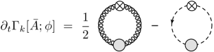
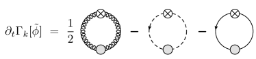
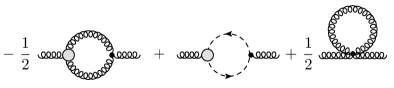
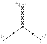
We begin with the FRG representation, which has also been used in Braun:2007bx ; Marhauser:2008fz ; Braun:2010cy ; Eichhorn:2011gc , for QCD-related reviews see e.g. Litim:1998nf ; Berges:2000ew ; Polonyi:2001se ; Pawlowski:2005xe ; Gies:2006wv ; Schaefer:2006sr ; Igarashi:2009tj ; Rosten:2010vm ; Braun:2011pp . We write the flow equation for the Yang–Mills effective action, , at finite temperature as
where the integration involves the respective gluon and ghost modes. Further, , with being the infrared cut-off scale. The diagrammatic representation given in Fig. 1.
The momentum integration measure at finite temperature is given by
| (19) |
where the integration over turns into a sum over Matsubara frequencies . Both, gluons and ghosts have periodic boundary conditions, , which is reflected in the Matsubara modes with a thermal zero mode for . Naturally, at vanishing temperature we have . The full field-dependent propagator for a propagation from the fluctuation to is given by
| (20) |
In short, we use
| (21) |
for the gluon and the ghost propagator, respectively. In (20) we also introduced the regulator function in field space, , with
| (22) |
The above entails that (LABEL:eq:funflow) only depends on the propagators of the fluctuations evaluated in a given background . This also holds for the flow of the background effective action . For more details we refer the reader to Fister:2011uw ; Fister:2011um ; Fister:Diss and Appendix A.
The effective Polyakov loop potential is given by
| (23) |
where for sufficiently large and sufficiently smooth regulators, see Fister:2011uw ; Fister:2011um ; Fister:Diss . We conclude that the computation of with FRG-flows only requires the knowledge of the (scale-dependent) propagators , see Braun:2007bx ; Braun:2010cy .
II.4 DSE for the Polyakov Loop Potential
The DSE for Yang–Mills theory relevant for the Polyakov loop potential is that originating in a derivative of the effective action with respect to the -background at fixed fluctuation. It can be written in terms of renormalised full propagators and vertices and the renormalised classical action. The latter is written as
| (24) |
with finite wave functions, coupling and gauge parameter renormalisation and renormalised fields , coupling and gauge fixing parameter . We have due to the non-renormalisation of the gauge fixing term. Moreover, background gauge invariance of the background field effective action (6),
| (25) |
and non-renormalisation of the ghost-gluon vertex Taylor:1971ff ; Lerche:2002ep leads to
| (26) |
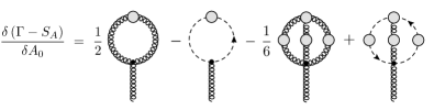
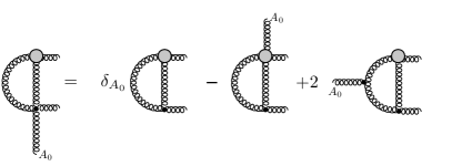
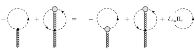
The above arguments yield the DSE for the Polyakov loop potential, schematically written as
| (27) |
and the diagrammatic representation given in Fig. 2.
In (27) and Fig. 2 we have used the renormalised classical vertices
| (28) |
at and
| (29) |
due to (26). The mixed three-point vertices in (28) have one background leg and two fluctuation legs and differ from the standard vertices: they are -derivatives of the related fluctuation-field propagator. Using from (26) it follows that the vertices in (28) have renormalisation group properties of fluctuation two-point functions, signaled by and , respectively. The two-point function property also entails that the gluonic vertex contains a piece from the gauge fixing term proportional to and the ghost-gluon vertex also involves the gauge field derivative of and not only .
The mixed four-point vertices in (29) have one background leg and three fluctuation legs and have the renormalisation group properties of the related fluctuation three-point functions multiplied by , signaled by and , respectively. The latter follows from in (26). The ghost-gluon four-point function stems from the background field dependence of the Faddeev-Popov operator , and causes an additional two-loop term in the DSE not present in the pure fluctuation DSE.
At asymptotically large momenta the finite wave function renormalisation are related to the normalisation of the two point functions with
| (30) |
Effectively this would amount to using propagators with
| (31) |
Applying the DSE (27) to constant backgrounds we are finally lead to the DSE equation for the effective Polyakov loop potential with
| (32) |
with (27) or Fig. 2 for the right hand side of (32). This equation is similar to the standard DSE for the fluctuation fields with the exception of the two-loop ghost contribution, only the vertices differ. In particular there is a contribution from the gauge fixing vertex which gives a perturbative one-loop contribution to the potential. The external field is a background gluon field with only a temporal component . This is reflected in the projections, see Appendix B. We conclude that the computation of only requires the knowledge of the propagators and of the full three-point functions and in a constant background.
II.5 2PI-Representation for the Polyakov Loop Potential
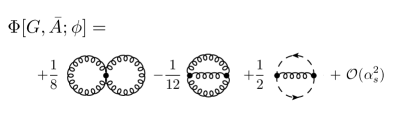
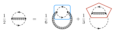
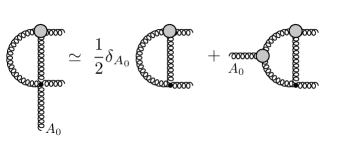
Now we extend our discussion to the 2PI approach, Luttinger:1960ua ; Lee:1960zza ; Baym:1962sx ; deDominicis:1964zz ; Cornwall:1974vz , for applications to gauge theories see e.g. Blaizot:1999ip ; Blaizot:1999ap ; Blaizot:2000fc ; Braaten:2001vr ; Arrizabalaga:2002hn ; Mottola:2003vx ; Carrington:2003ut ; Berges:2004pu ; Andersen:2004re ; Carrington:2007fp ; Reinosa:2007vi ; Reinosa:2008tv ; Reinosa:2009tc and the relation to the FRG-approach, see Blaizot:2010zx ; Carrington:2012ea . Its application will simply lead to a convenient resummation scheme for the DSE-equation for the Polyakov loop potential (32) derived in the last chapter: The functional DSE for the effective action displayed in (27) and Fig. 2 follows from the 2PI generating functional
| (33) | |||||
where contains only the 2PI pieces and are the gluon vacuum polarisation and ghost self-energy, respectively. Here, for the sake of notational simplicity we have set the renormalisation factors . The two-loop diagrams of are displayed in Fig. 3. The 1PI effective action is then given with
| (34) |
with the stationarity condition
| (35) |
i.e. the effective action is the 2PI-effective action evaluated on the gap equation. Now we take the derivative w.r.t. of in its 2PI-representation given in (34). The derivative acts on the explicit -dependence in the classical vertices as well as in the propagators. The latter terms, however, vanish due to the gap equation displayed in (34), thus,
where, by comparison with (27), Fig. 2, the last term simply is
Eq. (II.5) can be proven in any order of a given 2PI-expansion scheme such as 2PI perturbation theory or the -expansion. For example, the two-loop terms in , depicted in Fig. 3, provide the right hand side in (II.5) with classical vertices only. In the present work this is the approximation we shall use for the explicit computations. In any case we conclude that for the present purpose of studying the Polakov loop potential the 2PI-representation and DSE-representation are quite close and we shall make use of the similarities. Note that this similarity does not hold for e.g. dynamics of a given system where conservation laws such as energy and particle number conservation play a rle. Then, using self-consistent 2PI-schemes is mandatory.
III Confinement Criterion
The requirement of a confining potential at low temperatures restricts the possible infrared behaviour of low-order correlation functions: The FRG representation of constrains the behaviour of the propagators, and, furthermore, the DSEs and 2PI-equations constrain the three-gluon vertex as well.
First we discuss the restriction of the infrared behaviour of the propagators that follows from the FRG, (LABEL:eq:funflow). The present FRG-discussion extends and sharpens the criterion given in Braun:2007bx . There, the flow equation (LABEL:eq:funflow) was rewritten in terms of a total derivative and a term proportional to . Schematically this reads
| (38) | |||||
The second line can be understood as a renormalisation group (RG)-improvement as it is proportional to . Moreover, the -integrals of both lines on the right hand side are independent of the choice of the regulator as the integral of the first line caries this property trivially. In Braun:2007bx these arguments have been used to drop the second line in (38) as a correction term. This leads to, see Braun:2007bx ,
| (39) |
which reads for the Polyakov loop potential
| (40) |
as tends to zero exponentially for large initial cut-off scales . Note also that the approximation (40) has been used in Fukushima:2012qa ; Kashiwa:2012td . For confinement at small temperatures, , the potential is computed from the small momentum regime with where the propagators are given by for gluon and ghost with the scaling exponents and , respectively. It has been shown in Braun:2007bx that confinement enforces
| (41) |
in the approximation (40).
The suppression argument concerning the RG-improvement term presented above was tested in Braun:2007bx . There, the -propagators computed in Fischer:2008uz with an optimised regulator have been used. In the spirit of the suppression argument the potential was computed with the -propagators but with exponential regulator functions which facilitates this specific computation. It has been checked that the RG-improvement term indeed is small. We have now extended the analysis to a fully self-consistent computation with the thermal propagators from Fister:2011uw ; Fister:2011um ; Fister:Diss . Surprisingly, the RG-improvement term turns out to be large even though it has only a small impact on the phase transition temperature. This relates to the fact that in the non-perturbative regime RG-improvements are not parametrically suppressed by a small coupling and suppression arguments have to be taken with care. This mirrors the 20-30% percent deviation of the standard DSE-results for the ghost and gluon propagators at about 1GeV in comparison to lattice results, being linked to the dynamics which drives the phase transition. In the related DSE-approximations the two-loop term in Fig. 2 is dropped. This also implies that related approximation schemes in the 2PI-approach have to be evaluated with care.
Here, we take into account the full flow and note that all loop diagrams in (LABEL:eq:funflow) finally boil down to computing
| (42) |
where is the two-dimensional spherical surface and the dimensionless function is structurally given by
| (43) |
where and . In (43) we do not include the overall minus sign of the ghost contribution. The function stands for the respective scalar parts of the regulator functions. The choice of the regulators is at our convenience. For the present discussion (not so much for numerics) it is most convenient to choose -independent and -symmetric regulators,
| (44) |
The terms
| (45) |
with , are temperature corrections related to the Polyakov loop. Their impact on the phase transition has been discussed in detail in Section II.2. The important property in the present context is their decay with powers of the temperature for . At vanishing temperature we regain -symmetry and . In terms of scaling coefficients at vanishing temperature,
| (46) |
the corresponding propagators exhibit non-thermal mass gaps for . Note that the prefactor carries the momentum dimension . Hence, for we can ignore in the corresponding propagator for as it is suppressed with (potentially fractional) powers of . In turn, for propagators with field modes with the temperature correction may play a rle. However, for the time being we treat all of them as sub-leading corrections and discuss them later for the field modes with . This amounts to
| (47) |
for the present purpose. The integrands in (43) have the limits
| (48) |
where we remark that implies both and . Computing the expression (42) leads to a deconfining potential in : Taking a derivative w.r.t. it vanishes at and the center-symmetric points, i.e. where the Polyakov loop vanishes, . The second derivative is positive at while it is negative at the center-symmetric points.
Hence, with (47) the single loops in (LABEL:eq:funflow) give deconfining potentials. However, the ghost contribution has an overall minus sign. Therefore, the ghost contribution provides a confining potential. This already entails that the Polyakov loop potential in covariant gauges requires the suppression of the gluonic contributions.
In fact the same mechanism is at work in the DSE representation. Restricting ourselves to the one-loop terms for the moment, the gluonic modes give a deconfining potential whereas the ghosts yield a confining contribution. A simple mode counting shows, that the transverse gluons must be suppressed w.r.t. the ghosts for confinement to be present. This is also seen in Appendix B. In other words, with the assumption (47) the necessary condition for confinement is that
| (49) |
where the second condition guarantees for smooth that the ghost contribution dominates the trivial contribution of the gauge mode which is precisely , where is the one-loop perturbative potential, see (108) in Appendix B. In terms of the scaling coefficients introduced in (46) this translates into
| (50) |
where are the anomalous dimensions of the chromomagnetic and chromoelectric gluon, respectively. Eq. (49) is a sufficient condition for confinement in Yang–Mills propagators (with the assumption (47)) as it leads to a vanishing order parameter, the Polyakov loop expectation value. Note also that it has been shown Fischer:2006vf ; Fischer:2009tn within a scaling analysis that has to hold in the infrared. With this additional information we deduce that (49) encompasses the condition (41) derived in Braun:2007bx : For the minimal choice we get from (41) the condition which satisfies (50).
These conditions can be tested in toy models, in which the gluon propagator is suppressed very mildly, whereas the ghost propagator is trivial. This choice is the minimal satisfaction of the confinement criterion (49). Anticipating the final expressions for the FRG and DSE representations of the Polyakov loop potential, the immanence of confinement at sufficiently low temperatures is shown numerically in Appendix C.
The infrared limits (49) leading to the scaling coefficients (46) are satisfied, as they must, by the existing solutions in the literature, for a detailed overview over the solutions found on the lattice and in the continuum see e.g. Fischer:2008uz . The different solutions vary in the deep infrared. The decoupling solution, found on the lattice and in the continuum, exhibits a trivial ghost and a finite, non-vanishing gluon propagator, where the continuum allows for a scaling solution with a vanishing gluon propagator and an enhanced ghost propagator. In terms of the scaling exponents (46) the decoupling solution translates to and , the scaling solution shows with Zwanziger:2001kw ; Lerche:2002ep ; Pawlowski:2003hq . We stress again that both types meet the criterion (50) and exhibit confinement. In the computations presented below we have tested, that the type of solutions does not affect the critical physics at the confinement-deconfinement transition, neither qualitatively nor quantitatively. This is expected, as the relevant range for the phase transition is the mid-momentum region, where both decoupling and scaling solutions agree quantitatively.
We close this section with a discussion of the consequences and implications of (46) and (49): Note first that confinement not only implies a vanishing order parameter but also constrains other observables such as its correlations. The evaluation of these observables in terms of the propagators (and higher vertices) may lead to further, tighter constraints for the propagator. This point of view is interesting for model computations as there the above condition (49) is only a necessary one for deciding whether the model is confining or not. For example, one can easily construct models for Yang–Mills theory that have massive Yang–Mills propagators and a trivial ghost propagator at vanishing temperature. This can be parameterised as
| (51) |
Such a combination of propagators leads to a vanishing Polyakov loop expectation value but lacks the necessary positivity violation in the gluon system. It could model Yang–Mills theory in the Higgs phase but not in the confining phase. Note that it is precisely this feature which distinguishes the decoupling solution in Landau gauge Yang–Mills theory with from a massive solution put down in (51).
IV Confinement in Yang–Mills-Matter Systems
The confinement criterion discussed in the last section leads to a simple counting scheme for general theories. In the present section we put it to work in full dynamical QCD with fundamental or adjoint quarks, see e.g. Braun:2009gm ; Pawlowski:2010ht ; Braun:2011fw ; Braun:2012zq , as well as in the Yang–Mills–Higgs system with Higgs field in the fundamental or in the adjoint representation coupled to Yang–Mills theory, formulated in the Landau gauge, e.g. Fister:2010ah ; Fister:2010yw ; Macher:2010di ; Alkofer:2010tq ; Macher:2011ys . This also serves as a showcase for the general simple counting schemes which has emerged by now.
We concentrate on the one flavour case (Higgs or quark), the generalisation to many flavours is straightforward. Note also in this context that the present confinement criterion constrains the physics properties of a potentially confined phase, it does not prove or disprove its dynamical existence in the theory at hand. For example, it is well-known that for a sufficiently large number of quark flavours in the fundamental or adjoint representation, QCD ceases to be confining. Then the propagators simply do not satisfy the confinement criterion.
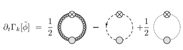
We start with a discussion of the adjoint Higgs (one flavour) with the action
| (52) |
The flow equation for the Polyakov loop potential is depicted in Fig. 4.
We have already seen that in the Landau gauge the question of a confining potential at low temperatures boils down to counting the massless modes including the prefactors and from the loops of bosons and fermions, respectively, where we normalise the standard boson loop with the prefactor to one. In the symmetric phase at high temperatures, all modes are effectively massless for our counting: All vacuum masses are suppressed with the temperature. Our counting is normalised at the (one-loop) Polyakov loop potential in Yang–Mills theory which is computed from 2 boson loops, that are related to the physical transversal gauge modes; the third transversal contribution and that of the longitudinal gauge mode are canceled by the ghost contribution,
| (53) |
Hence, in the present case we have contributions from the gauge field (4 vector modes), ghost contributions (relative factor for the loop), and Higgs contribution. This amounts to an overall factor of for the symmetric phase of the adjoint Yang–Mills–Higgs system,
| (54) |
This has to be compared with the counting factor for the pure Yang–Mills system, leading to the one-loop Polyakov loop potential Weiss:1980rj ; Gross:1980br , given in Appendix (108). The one-loop potential for the Yang–Mills-adjoint Higgs system, , is hence given by
| (55) |
In turn, in the fully-broken phase of the Yang–Mills–Higgs system, we have one radial massive (away from the phase transition) Higgs mode with expectation value and Goldstone bosons. In the glue sector, gauge bosons acquire an effective mass due to the non-vanishing expectation value of the Higgs field. In the Landau gauge this leads to massive propagators for the transversal modes, if the theory is evaluated at the expectation value of the Higgs field. The gauge mode, even though it also acquires a mass, is effectively massless: Its propagator, evaluated at the expectation value of the Higgs, reads
| (56) |
and, for Landau gauge, , it only contributes via the longitudinal part of the regulator proportional to in the flow equation or via the gauge-fixing part proportional to in the DSE and 2PI formulation. We conclude that the gauge mode in the Landau gauge stays effectively massless in any phase. Together with the remaining massless gauge boson we have massless modes in the gauge boson sector.
For example, in we have and without loss of generality we take
| (57) |
leading to
| (58) | |||||
Hence we have massive modes. This includes the gauge mode which, however, is effectively massless in the Landau gauge due to (56). Note that the latter fact is special to Landau gauge. In the unitary gauge also the gauge mode gets massive as does the Faddeev–Popov operator.
We proceed to the Polyakov loop potential. First we note that the massive radial Higgs mode effectively blocks one colour direction with projection operator . For the transversal gauge field propagators, the situation is exactly the opposite. All the modes in the subspace are massive and the massless transversal colour direction is that in direction . Since we are finally only interested in the sign of the sum of the contribution we simply remark that adding one of the three transversal massless gauge boson conbributions to the Higgs effectively restores the Higgs boson contribution in the symmetric regime. We also still have the trivial contribution from the gauge mode. Moreover, the ghost is essentially unchanged as in the pure Yang–Mills case, it still has a massless dispersion. We conclude that due to the relative sign of the ghost contribution the Higgs, the effectively ’restored’ Higgs contribution and the gauge contribution are canceled by the ghost contribution. This is the manifestation of the Higgs–Kibble mechanism for the Polyakov loop potential in the Landau gauge: The apparently massless contributions cancel each other including those of the Goldstones. In the unitary gauge the Goldstone modes are included in the longitudinal gauge field modes, which would be massive and would have dropped out due to their masses.
What is left is the contribution from the remaining two massless transversal gauge bosons with the colour direction . For gauge fields with or this provides a deconfining contribution to the Polyakov loop potential which counts as in the present counting. Again, all this is apparent in the -example. Adding all the massless contributions we arrive at
| (59) |
Hence, the Polyakov loop potential for the Yang–Mills-adjoint Higgs system in the Higgs phase is deconfining, albeit suppressed with order .
We close the analysis on the Yang–Mills-adjoint Higgs system with a remark on a confining phase in this theory: In this phase all gluon modes are expected to be gapped, except for the gauge mode. Keeping the other modes unchanged, the sum in (59) turns negative implying confinement,
| (60) |
Note however, that (59) includes gapped Higgs modes. If these modes became massless they would counter-balance the gapping of the confined gluons. We conclude that gapped Higgs modes are required in the confined phase. This is a reminiscent of the expectation in Yang–Mills-quark systems where one usually expects chiral symmetry breaking in the confined phase.
Let us compare this with the situation in QCD with adjoint fermions. There, the action reads
| (61) |
The flow equation for the Polyakov loop potential is depicted in Fig. 5.
The fermionic one-loop contribution to the Polyakov loop potential reads
| (62) |
where we have used that for constant fields , and is the identity in spinor space with . The fermionic contributions are deconfining as the quarks have anti-periodic boundary conditions, , and, hence, the Matsubara frequencies are shifted: . This entails that the Polyakov loop potential is shifted by a factor :
| (63) |
which is deconfining with the same strength as the Yang–Mills potential. This argument stays valid beyond one loop. For large temperature we conclude that the adjoint quarks for large temperatures lead to contributions,
| (64) |
This has to be compared with for the pure Yang–Mills system, leading to the one-loop Polyakov loop potential , (108). The one-loop potential for the Yang–Mills-adjoint Higgs system, , is hence given by
| (65) |
In turn, in the chirally broken phase all quarks are massive and their contributions are removed from the Polyakov loop potential. The glue sector is qualitatively the same as in Yang–Mills theory, the transversal modes are gapped, while the gauge mode is effectively massless. Hence, we are lead to
| (66) |
the theory is confining in clear contradistinction to the Higgs phase in the Yang–Mills-adjoint Higgs system. Note also that this directly implies no confinement without chiral symmetry breaking for QCD with adjoint quarks if the gapping in the quark sector relates to chiral symmetry breaking. Strictly speaking, however, (66) implies no confinement without gapped quarks. In turn, in Braun:2012zq it has been shown that confinement, that is a vanishing expectation value of the Polyakov loop, leads to chiral symmetry breaking. These two results tightly link chiral symmetry breaking and confinement for QCD with adjoint quarks.
In a potential chirally symmetric low energy phase, or better massless low energy phase, we have
| (67) |
which relates to a deconfining Polyakov loop potential.
We close the section with a discussion of matter in the fundamental representation coupled to Yang–Mills theory. There, center symmetry is explicitly broken. The Polyakov loop is not an order parameter anymore and the question of the confining or Higgs phase has to be answered differently. Indeed, we know that on the lattice these two phases are not well-separated Osterwalder:1977pc ; Fradkin:1978dv ; Kertesz:1989 . A full discussion of this goes far beyond the aims of the present contribution. Here we simply discuss our counting scheme and compare its outcome for the Yang–Mills-fundamental Higgs system with physical QCD. The action of the Yang–Mills-fundamental Higgs system reads
| (68) |
similarly to the action for an adjoint Higgs, but with the group trace in the fundamental representation, the Higgs living in the . For , the Higgs is a complex 22-matrix,
| (69) |
The diagrammatics of the flow equation for the Polyakov loop potential does not change in comparison to the adjoint Higgs and is depicted in Fig. 4, the last loop now involving a trace in the gauge group in the fundamental representation.
The fundamental Higgs has modes due to its -representation. In the symmetric phase at high temperatures all of them are effectively massless. The group traces, however, are in the fundamental representation of , and, hence, they are suppressed by a factor (in the large limit) in comparison to the traces in the adjoint representation. More precisely, the multiplicity of the non-vanishing eigenvalues of is relatively suppressed with . The fundamental representation also leads to different eigenvalues of , see in particular Braun:2009gm . For example, for we have for contributions in the adjoint and fundamental representation
| (70) |
which can be nicely tested for the one-loop contributions. Note also, that the -mode does not couple to the -gauge field and is a pure -potential. In (70) the factor on the right hand side signals the explicit breaking of center symmetry. This also means that one should not simply add the counting factors of contributions in different representations. We merely remark here that as long as the contributions from the center-symmetry breaking sector is small, one may still have a phase transition of the order determined by -symmetry. The larger the contributions of the center-symmetry breaking sector are, the weaker the transition or finally the cross-over gets. The interpretation of the latter as distinguishing different phases is not clear.
Restricting ourselves to the center-symmetric field modes we get for large temperatures
| (71) |
the counting of pure Yang–Mills theory. This entails that the Polyakov loop potential of the glue sector is deconfining. At one-loop we have a deconfining total potential,
| (72) |
In turn, in the fully-broken phase of the Yang–Mills-fundamental Higgs system we have one radial massive (away from the phase transition) Higgs mode with expectation value which does not couple to the gauge field. We also have Goldstone bosons. In the glue sector, all gauge bosons acquire an effective mass due to the non-vanishing expectation value of the Higgs field. In the Landau gauge this leads to massive propagators for transversal gauge modes and massless gauge modes. The ghost is massless, and in summary this leads to
| (73) |
a confining potential for the glue sector. The massless modes give a center-symmetry breaking potential, which, however, is suppressed by a factor for large . Whether for finite one has a cross-over or still a first order, (), or second order, , phase transition is decided dynamically and is not accessible by the present counting. Evidently, however, is the existence of a confining potential in the large -limit. In this limit the pure glue sector dominates the Polyakov loop potential due to the -suppression of the Higgs contributions.
Finally we compare the situation in the Yang–Mills-fundamental Higgs system with physical QCD with fundamental quarks, the most interesting and most studied system. Its action is given by
| (74) |
and the flow equation for the Polyakov loop potential is depicted in Fig. 5. The Higgs in the fundamental representation breaks center symmetry in the same way a fundamental quark does, and the Polyakov loop potential shows no phase transtion. The order parameter is a smooth function of temperature similarily to two-flavour QCD studied in Braun:2009gm . One may be tempted to interpret the behaviour in terms of a cross-over; however, the Wilson loop shows no area law which is in accord with the behaviour of the Polyakov loop. As for the Higgs the pure glue sector shows the counting (73). The part of the potential computed from the massless fermionic modes satisfies
| (75) |
and with anti-periodic boundary conditions for the fermion we get
| (76) |
where is the potential of one bosonic mode in the fundamental representation. In the large -limit the fermionic contributions are suppressed (unless the number of flavours increases with the number of colours) and yield a confining theory with a first order phase transition. At finite , and in particular , we expect a significant influence of the fermions at temperatures above the chiral symmetry breaking scale. Below this scale the fermionic contributions are more and more suppressed and we are left with the pure glue counting.
V Results for the Polyakov Loop Potential and
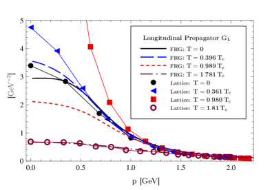
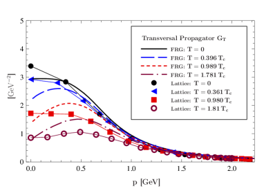
Here, we compute the Polyakov loop potential within the FRG, DSE and 2PI representation with the propagators at vanishing and finite temperatures obtained from the FRG in Fister:2011uw ; Fister:2011um ; Fister:Diss . There, the finite temperature propagators for all cut-off scales have been computed on the basis of a given set of propagators at vanishing temperature and vanishing cut-off scale . This minimises the systematic error of a given approximation: Only the difference of the - to the -propagator and the thermal to the -propagator, respectively, is sensitive to the approximation. The results for the Matsubara zero mode for the longitudinal and transversal propagator, , are displayed in Fig. 6 and Fig. 7, respectively, for some temperatures below and above the phase transition. They are compared to lattice results Maas:2011ez ; Maas:2011se .
The FRG results have been obtained in a slightly modified approximation in comparison to Fister:2011uw ; Fister:2011um , see Fister:Diss . We resort to the additional approximation
| (77) |
which has proven to be an accurate approximation in former studies Maas:2005hs ; Cucchieri:2007ta ; Fischer:2010fx ; Fister:Diss . For the present purpose of computing the Polyakov loop potential this is a quantitatively reliable approximation as the finite temperature effects in the propagators decay already rapidly for momenta with in the FRG computations. We conclude that already the first Matsubara mode is close to the zero mode evaluated as in (77). Note however, that this does not apply to thermodynamical quantities as already pointed out in Fister:2011uw ; Fister:2011um ; Fister:Diss , for non-relativistic analogues see Boettcher:2012cm ; Boettcher:2012dh .
V.1 Results from the FRG
As discussed before the flow equation has the minimal representation for the Polyakov loop potential as it only requires the propagators in a given background. The present computations improves upon that in Braun:2007bx ; Braun:2010cy with the use of the thermal propagators.
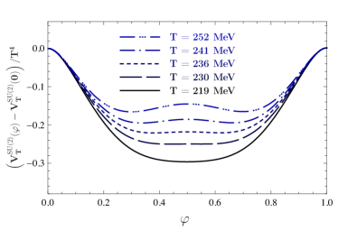
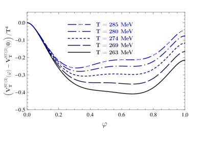
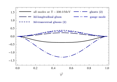
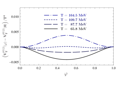
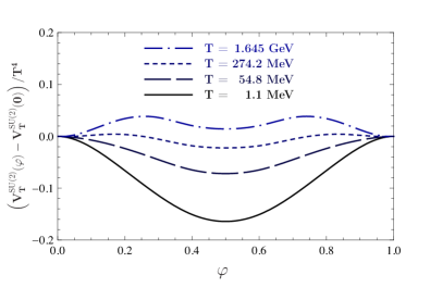
In addition, further emphasis is put on the regulator-independence, see Appendix A. The potential is depicted for temperatures above and below the critical temperature for in Fig. 8, and for in Fig. 9. Without loss of generality we shift the potential trivially such, that , and divide by the canonical dimension to simplify the comparison, as the Weiss potential in this normalisation is independent of the temperature.

From these potentials the confinement-deconfinement critical temperatures are determined at
| (78) |
The absolute temperatures in (78) are set in comparison to absolute scales of the lattice propagators with a string tension
| (79) |
which leads to the dimensionless ratios of
| (80) |
For our result is in quantitative agreement with the lattice results,
| (81) |
which yield the ratios
| (82) |
For a review on lattice results see e.g. Lucini:2012gg . Our relative normalisation is taken from the peak position of the lattice propagators in Maas:2011ez ; Maas:2011se ; Fischer:2010fx . Note however, that this normalisation has an error of approximately which is reflected in the errors in (78).
In turn, for , the critical temperature is significantly lower than the lattice temperature in (81). This is linked to the missing back-reaction of the fluctuations of the Polyakov loop potential, see Section II. Including the back-reaction in the Landau gauge flow leads to a transition temperature of
| (83) |
see Spallek . More details will be presented elsewhere. This result agrees quantitatively with the lattice temperature as well as with the result obtained with flows in the Polyakov gauge Marhauser:2008fz which also reproduced the correct critical scaling of the Ising universality class.
V.2 Results from DSE & 2PI


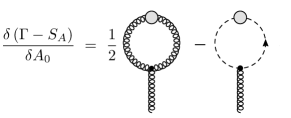
The full computation of the Polyakov loop potential (32) from the DSE including the two-loop terms requires the knowledge of the full three-gluon vertex and the full ghost-gluon vertex in the presence of an -background, see (27) and Fig. 2. Moreover, one has to compute two-loop diagrams in the presence of such a background. Here, we present a simple resummation scheme for effectively computing these terms in an expansion of the Polyakov loop potential in full propagators and full vertices. The simplest way to do this is to consider the 2PI-hierarchy in Fig. 3 up to two-loop. As it also provides some additional information about the resummation scheme we also present a derivation solely within the DSE-approach in Appendix D.
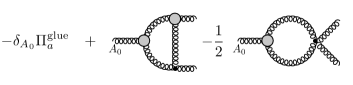
The two-loop terms in can be rewritten in terms of one-loop diagrams with full propagators and gluon vacuum polarisation and ghost self-energy, see Fig. 10 and Fig. 11, respectively. We easily identify the corresponding diagrams in . The first gluonic diagrams in as in Fig. 3 can be rewritten in terms of (-1/6 of) the gluonic part of the vacuum polarisation contracted with the full gluon propagator, which is depicted in Fig. 12.
Then, the last two-loop diagram in , Fig. 3, is rewritten in terms of the missing ghost contribution to the gluonic vacuum polarisation in Fig. 12, and (-1/3) of the ghost self-energy contracted with the full ghost propagator, see Fig. 13. Both terms are subtractions to the 1PI-terms in the 2PI effective action, (33). This leads to the final form of the effective action,
with
| (85) |
comprising the contributions of order in a perturbative 2PI ordering as well as a tadpole contribution. As mentioned before, a derivation of (V.2) within the DSE-approach can be found in Appendix D. In the explicit computations presented below we will drop . The tadpole term is set to zero at in standard renormalisation schemes as it is a mass-contribution. Its thermal -dependent contribution is suppressed by roughly one order of magnitude, , relative to the contribution of the full tadpole in the final expression, see (V.2). Moreover, its -dependent part solely contributes to the defined in (15) which we have consistently dropped in the explicit computations presented here.
In conclusion, with , we have arrived at a representation (V.2) of the effective action which is manifestly RG-invariant. Indeed, both the first and the second line are separately RG-invariant. One is tempted to even drop the second line in (V.2) in a first computation. However, even though this should not have a qualitative impact on the phase transition temperature, it turns out to have a big impact on the amplitude of the potential. We have checked this within the flow equation for the Polyakov loop potential: (V.2) resembles (38). The first lines agree up to the normalisation at which is trivial. Thus, we deduce that up to the above normalisation the second line of (V.2) is identical to
where the right hand side has the manifest RG-invariance due to being an integrated flow. We have already discussed in Section III below (41) that the integrated flow in (V.2) is not negligible for the potential even though it does not play a major rle for the phase transition temperature. We emphasise that a detailed comparison of the different approximations is of great interest for phenomenological applications in QCD, and in particular also for approaches to QCD within Polyakov-loop enhanced low energy models, see e.g. Meisinger:1995ih ; Pisarski:2000eq ; Fukushima:2003fw ; Mocsy:2003qw ; Dumitru:2003hp ; Ratti:2005jh ; Ghosh:2006qh ; Schaefer:2007pw ; Sakai:2008py ; Skokov:2010wb ; Herbst:2010rf . This analysis is beyond the scope of the present work and will be presented elsewhere.
Hence, we also consider the second line in (V.2) and use the scheme-independence of the result in (V.2) to further simplify the computation: With the Dyson equation,
| (87) |
we rewrite the DSE for the effective potential, (32), in terms of the one-loop diagrams in Fig. 2 and the rest,
| (88) | |||||
After performing the Lorenz traces in the second line of (88), the remaining operator traces are simply of the form
| (89) |
where , are the respective wave functions, see (11). The abbreviation stands for the the -derivative of ,
Now we minimise the size of the contributions from the second and third line in (88) close to the transition temperature by using an appropriate RG-scheme, that is an appropriate renormalisation scale with at . Since we are interested in the physics at temperatures at about this already implies GeV. We can further restrict this choice by demanding that for and we have
| (90) |
Eq. (90) minimises the integrand in the momentum integrals in the second and third line in (88) at the momenta with the largest contributions. In (90) a sum over the chromoelectric and the two chromomagnetic polarisations is understood. For temperatures MeV (90) is solved for
| (91) |
We also can investigate the -dependence of the splitting related to the normalisation with . To that end we apply the related variation to (90), that is the operator and obtain from (90)
| (92) |
with
| (93) |
Again this yields GeV which entails that the contribution of the second and third line in (88) can be minimised for temperatures close to along (90). Note also that, since the differences are marginal, it can also be evaluated at as a first good approximation. There we have and (90) simplifies to
| (94) |
which is satisfied for GeV as well. The constraint (90) fixes the RG-scale with GeV close to and in the temperature regime between MeV. Moreover, it can be shown that a variation of in this regime by 100% only leads to changes of the results on the percent level, in particular does not change at all. For the numerical computations we have chosen
| (95) |
Note that this RG-scheme effectively normalises the propagators used in the DSE and 2PI hierachy to one at the RG-scale, . At finite temperature this only holds approximately.
In summary we have derived that for appropriately chosen RG-schemes with the DSE for the Polyakov loop potential effectively boils down to a simple one-loop form, depicted in Fig. 14.
In Appendix B the one-loop diagrams in Fig. 14 are reduced to
| (96) | |||||
where are the propagators for the chromoelectric gluon, the chromomagnetic gluon and ghost propagators normalised at vanishing temperature at the point , and the first term originates in the gauge mode. The evaluation of (96) leads to the potential depicted in Fig. 15 for and Fig. 16 for . From those the confinement-deconfinement critical temperature is determined at
| (97) |
which gives
| (98) |
These results are in quantitative agreement with the FRG results, (78), and can be compared with lattice results in (81) and (82).
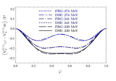
We close this chapter with a comparison of the temperature-dependence of the FRG and DSE/2PI potentials. Note that the DSE/2PI computation presented here approximately also takes into account the integrated RG-improvement in (V.2) for temperatures about the phase transition temperature. Hence, not only but also the potentials themselves should agree quantitatively for temperatures close to . We also remark that for the present approximation may lose its quantitative character as the normalisation of the ghost and gluon propagators changes rapidly for momenta important for the Polyakov loop potential. In Fig. 17 we only show the comparison of the potentials for , as that for simply follows from an weighted sum over -potentials, cf. Appendix B. The potentials agree quantitatively to a surprising level of accuracy which confirms the quantitative nature of both, FRG and DSE/2PI-computations. For temperatures there is a significant deviation as the DSE/2PI-approximations used here loses its quantitative nature. Note that this also holds for the approximation (40). In turn for both approaches converge towards the perturbative potential. The present approximation in the DSE/2PI-approach is easily improved by taking into account the two-loop terms in (88). The discussion of the respective results goes beyond the scope of the present work and will be presented elsewhere.
VI Conclusions
We have studied the confinement-deconfinement phase transition of static quarks with the effective potential of the Polyakov. The position of the minima signals the presence or absence of confinement, as they can be related to the free energy of a single quark. The potential itself was computed in the background field formalism in the Landau–deWitt gauge. This allows for the use of Landau gauge propagators at vanishing background, which had been obtained previously in the framework of the FRG Fister:2011um ; Fister:2011uw ; Fister:Diss . The study here was done within different non-perturbative functional continuum approaches, i.e. using FRG-, DSE- and 2PI-representations of the effective action.
In all variants we find a second order phase transition for and a first order transition for , as it is expected from lattice QCD. The corresponding temperatures agree quantitatively for all functional methods within the estimated error of approximately 10%, originating in the normalisation of the total momentum scale. The results including the lattice temperatures are summarised and discussed in Section V.1 and Section V.2. These results are stable w.r.t. the choice of scaling or decoupling type solutions for the propagators and, furthermore, to the variation of the regulator in the FRG approach. The critical temperature for from functional methods agrees quantitatively with the corresponding lattice temperature. For the critical temperature from functional methods is significantly lower than the lattice temperature. This is linked to the missing back-reaction of the fluctuations of the Polyakov loop potential, see Section II.2. Its inclusion leads to critical temperatures in quantitative agreement with the lattice results and the correct Ising-type critical scaling, see Marhauser:2008fz ; Spallek .
The dependence of the Polyakov loop potential on the individual gluon and ghost modes is easily tractable. This was exploited to derive a simple criterion for static quark confinement. For infrared suppressed gluon but not suppressed ghost propagators confinement is immanent at sufficiently low temperatures. Independent of the functional approach chosen above, this is due to the fact, that the two non-suppressed confining ghost modes always overcompensate the deconfining trivial gluon gauge mode. As a result of their suppression, the remaining transversal gluon modes decouple at temperature scales far lower than the suppression scale and confinement is realised.
This confinement criterion has also been applied to general Yang–Mills-matter systems with matter in the adjoint and the fundamental representation. For matter in the adjoint representation again an infrared suppressed gluon is mandatory. Moreover, the criterion is sensitive to the difference between Higgs phase and confined phase even though both phases have infrared suppressed gluons. For matter in the fundamental representation the matter part of the potential breaks center symmetry. Hence it is only possible to evaluate the relative importance of center symmetry modes and center breaking modes.
In summary the work establishes both on the qualitative and quantitative level the functional approach to confinement by means of the Polyakov loop potential. It only requires the computation and discussion of background-gauge propagators and hence allows a very simple access to structural questions such as the confinement mechanism as well to explicit analytic and numerical computations of the phase structure.
Acknowledgments — We thank Jens Braun, Astrid Eichhorn, Christian S. Fischer, Holger Gies, Jan Lücker and Axel Maas for discussions. This work is supported by the Helmholtz Alliance HA216/EMMI and by ERC- AdG-290623. LF is supported by the Science Foundation Ireland in respect of the Research Project 11-RFP.1-PHY3193 and the Helmholtz Young Investigator Grant VH-NG-322.
Appendix A Regulators
The regulator function introduced in the FRG approach can be chosen freely as long as it fulfills certain limits. Firstly, it must have the same tensor structures as the corresponding two-point function. Neglecting those tensors for the moment, must (i) regulate the propagator in the infrared, (ii) leave the full quantum theory for vanishing renormalisation group scale and (iii) suppress fluctuations at large scales to reduce to the classical action. Formally, these requirements are met by
| (99) | |||||
| (100) | |||||
| (101) |
The full theory is independent of the choice of , however, in truncations this may not be satisfied. This rules out certain forms of the regulator. Another restricting factor is the applicability in the computations, as some regulators are not feasible numerically.
For the thermal gluon and ghost propagators of Yang–Mills theory, four-dimensional exponential regulators,
| (102) |
with , have proven to be well suited for numerical purposes Fister:2011um ; Fister:2011uw ; Fister:Diss . Note however, that for the numerical computation of the Polyakov loop potential the regulator must not be too sharp, thus, , cf. Fister:Diss .
The regulation of the propagator in the infrared demands that is of approximately the same amplitude than the at each . This is ensured by a prefactor such, that
| (103) |
For the purpose presented here the precise form of is not crucial but lengthy, thus, for the exact definitions we refer the interested reader to Fister:2011uw ; Fister:2011um ; Fister:Diss . The results presented in section V.1 are obtained with regulators (103).
In order to test the (in)dependence of the Polyakov loop potential on the choice of the regulator, we have studied different functions and prefactors in the full regulator function. This was done for temperature-independent propagators, since not all choices of are viable for thermal effects.
The scale-dependency of the propagators, of both scaling and decoupling type, was obtained with (103) for Fister:2011uw ; Fister:2011um ; Fister:Diss . These results were, firstly, combined with self-consistent choices in the determination of the Polyakov loop potentials. Secondly, the Polyakov loop potential was computed with these propagators but with . Measured on the level of the confinement-deconfinement phase transition temperature of , we find good stability w.r.t. the variation of the regulators and, furthermore, w.r.t. scaling of decoupling type propagators, as all choices are within 5% deviation. Furthermore, we found that for different choices of the regulator in propagators and Polyakov loop potential, namely those which have relative shifts in the renormalisation group scale, the truncation effects may grow larger.
Appendix B One-Loop Diagrams in the DSE for the Polyakov Loop Potential
The one-loop diagrams are given in Fig. 14. Both couple the external temporal gluonic background to the fluctuating loop fields. For clarity we consider temperature-independent propagators first, before we decompose the tensor structures for the case of non-trivial temperature dependence of the propagators.
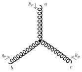
The gluon loop, depicted in Fig. 18(a), involves the three-gluon vertex with one background leg. At vanishing fields it is given by
| (104) |
where the second term originates from the background field dependence of the gauge fixing term, see (5). The classical vertex is given in Fig. 18(b).

For this very definition it is given by
At the gluon propagator has four degrees of freedom, three transversal modes and the longitudinal gauge mode, thus, at vanishing fluctuation fields and a constant background we can split the gluon propagator according to
| (106) |
where the first term is the non-trivial transversal part , whereas the second term represents the gauge mode. This is a consequence of the corresponding Slavnov–Taylor identitites: The quantum corrections to the propagator are transversal and, hence, the gauge sector is unchanged. Together with the background vertex (104) this leaves us with a contribution of the gauge sector
| (107) |
where the trace on the right hand side does not include a trace over Lorentz indices and gives , the perturbative one-loop potential. The latter is given by
| (108) |
where is the number of spacetime dimensions and are the eigenvalues of the generators of the gauge group spanned via the Cartan subalgebra. For the eigenvalues are . For and the background-independent propagators one can construct the potential according to the eigenvalues,
| (109) | |||||
The non-trivial part of the computation concerns the transversal part , which couples to the standard part of the three-gluon vertex, , given in (B). Note that at vanishing temperature the propagator is -symmetric, thus, it only depends on the absolute value of the momentum, not on the spatial and temporal components separately like at non-vanishing temperature, see (11).
For a purely temporal momentum the loop diagram in Fig. 18(a) translates to
| (110) |
where due to symmetry only the term survives, with and according to (30).
In (110) the factor counts the three coinciding transversal modes. For thermal propagators the projection is such, that it accounts for the chromoelectric and chromomagnetic modes. Thus, without repeating the computation along the lines of (110), we get the final expression for the loop diagram Fig. 18(a) as
| (111) |
with and being the chromoelectric and chromomagnetic gluon propagators with the normalisation at vanishing temperature given in (30).
Having the similiar structure as the gluon loop, the ghost loop is given in Fig. 19(a).
The first ingredient of this diagram is the classical ghost-gluon vertex as defined in Fig. 19(b). It is given by
| (112) |
Note that the ghost-gluon vertex involves an additional factor of compared to the vertex in standard Landau gauge, due to the appearance of the covariant derivative (instead of a plain derivative ) in the last term of (5).
The second component in the ghost loop is the full ghost propagator. It is a Lorentz scalar, thus, dropping the colour structure it is simply given by a scalar function . Thus, for trivial and non-trivial implicit temperature dependence of the propagator, the diagram attached to a purely temporal gluon field in Fig. 19(a) reduces to
| (113) | |||||
where . Due to symmetry, this only leaves the term
| (114) |
In combination with the gauge mode, the sum of the individual contributions yields the final expression for the DSE of the Polyakov loop potential (96).
Due to the different sign in the ghost loop and the gluon suppression the potential shows confinement for small temperatures. The additive contributions of the different modes, the chromoelectric, chromomagnetic, gauge modes from the gluon and the ghost modes, are illustrated in Fig. 20 at a temperature around the phase transition. For lower temperatures, the ghost contributions grow stronger and the transverse gluons decrease further. In contrast, for higher temperatures the propagator approach the perturbative forms, thus, the potential approaches the (deconfining) Weiss potential (108).
Appendix C Confinement for Mildly Suppressed Gluons
In this section we confirm the hypothesis made in section III in a numerical application for both approaches DSEs and the FRG. In these computations the ghosts are left trivial, thus, they give a confining potential which overcompensates the gauge mode, and both terms sum up to . We show, that already a soft suppression of transversal gluons yields a decrease of the deconfining effect such, that confinement is immanent at sufficiently low temperatures.
For the DSE we choose an ansatz, in which transversal gluons are suppressed for infrared momenta, thus,
| (115) |
The full result is given in Fig. 21, where clearly a confining potential is realised at low temperatures.
In the case of the FRG the suppression must also be present in the renormalisation group flow along the scale . Thus, a qualified ansatz is given by
| (116) |
The result for this ansatz is given in Fig. 22.
From these two examples we can infer, that indeed a mild gluon suppression is sufficient to yield a confining potential at low temperatures, as we claimed in section III. Nevertheless, the sum of gluonic, ghost and gauge modes is non-trivial, thus, we refrain from giving phase transition temperatures here, as these examples only serve as a proof of principle and are of no quantitative physical relevance.
Appendix D Direct resummation of the DSE-hierachy
In this appendix we provide the necessary steps for deriving (V.2) solely within the DSE-approach. Note that this simply amounts to using the ghost and gluon gap equations in the DSE hierarchy which is trivially implemented in the 2PI-approach. To that end we have to rewrite the two-loop diagrams in (27), Fig. 2. Similarly to the 2PI argument leading to (V.2) this diagram can be turned into a one-loop form within a resummation scheme which neglects some order -corrections to full vertices but takes into account full propagators. In the following we explicitly perform this analysis for the gluon two-loop diagram, the same steps can be trivially taken over for the ghost two-loop diagram: First, we note that the two-loop diagram has no contributions from the gauge fixing vertices proportional to which contributes in the one-loop diagram, see Appendix B. The reason is that the full and renormalised classical vertices involve more than 2 fluctuating fields . Moreover, the two-loop contribution can be seen as a vertex-correction diagram to the gluonic one-loop diagram, see Fig. 23.

The vertex correction can be rewritten in terms of a total -derivative, a three-gluon vertex diagram and a term which resembles (minus) the vertex correction, see Fig. 24. The only difference is that the leg is attached to the full vertex. Since the two fluctuating fields are attached to the additional propagator in the two-loop diagram, the original diagram and this one differ in order in the vertex. Hence, in the present approximation we identify it with (minus) the vertex correction. We also note that strictly speaking the last diagram in Fig. 24 only involves the -vertex originating in . However, the gauge fixing part does not contribute anyway as the vertex is contracted with two transversal propagators. Hence, for the sake of simplicity we will always use the full -vertices, but the gauge-part is projected out in the diagrams.
Moving the vertex correction to the left hand side side leads to the form Fig. 25 of the vertex correction, up to the vertex correction-terms of order . The first term on the right hand side of Fig. 25 is (minus) the three-gluon vertex part of the gluonic part of the gluon vacuum polarisation , see Fig. 10. We rewrite it accordingly and the right hand side takes the form displayed in Fig. 26,
| (117) |
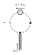
Upon closing the open -lines in Fig. 26 with the remaining gluon propagator the corresponding one-loop sub-diagrams constitute up to a factor in the tadpole diagram. As for the 2PI-derivation we drop this diagram. Inserting Fig. 26 into Fig. 23 we are led to Fig. 27.
Similar steps as above can be done for the ghost two-loop diagram. Here we simply note that the two ghost terms in the DSE Fig. 2 can be rewritten as displayed in Fig. 28. The first term on the rhs in Fig. 28 is the -derivative of the -term in (V.2). In turn, the two remaining terms equal
| (118) |
This is most easily seen by just comparing the perturbative two-loop diagrams in both expressions.
In summary the gluonic and ghost terms in the DSE add up to the total -derivative (V.2).
References
- (1) J. Braun, H. Gies, and J. M. Pawlowski, Phys.Lett. B684, 262 (2010), 0708.2413.
- (2) F. Marhauser and J. M. Pawlowski, (2008), 0812.1144.
- (3) J. Braun, A. Eichhorn, H. Gies, and J. M. Pawlowski, Eur.Phys.J. C70, 689 (2010), 1007.2619.
- (4) L. Fister and J. M. Pawlowski, (2011), 1112.5440.
- (5) L. Fister and J. M. Pawlowski, (2011), 1112.5429.
- (6) L. Fister, PhD thesis, Heidelberg University (2012).
- (7) R. Alkofer and L. von Smekal, Phys. Rept. 353, 281 (2001), hep-ph/0007355.
- (8) C. D. Roberts and S. M. Schmidt, Prog. Part. Nucl. Phys. 45, S1 (2000), nucl-th/0005064.
- (9) C. S. Fischer, J.Phys.G G32, R253 (2006), hep-ph/0605173.
- (10) C. S. Fischer, A. Maas, and J. M. Pawlowski, Annals Phys. 324, 2408 (2009), 0810.1987.
- (11) D. Binosi and J. Papavassiliou, Phys.Rept. 479, 1 (2009), 0909.2536.
- (12) J. M. Pawlowski, AIP Conf.Proc. 1343, 75 (2011), 1012.5075.
- (13) A. Maas, Phys. Rep. in press (2013), 1106.3942.
- (14) L. von Smekal, Nucl.Phys.Proc.Suppl. 228, 179 (2012), 1205.4205.
- (15) J. Braun, L. M. Haas, F. Marhauser, and J. M. Pawlowski, Phys.Rev.Lett. 106, 022002 (2011), 0908.0008.
- (16) C. Gattringer, Phys. Rev. Lett. 97, 032003 (2006), hep-lat/0605018.
- (17) F. Synatschke, A. Wipf, and C. Wozar, Phys.Rev. D75, 114003 (2007), hep-lat/0703018.
- (18) E. Bilgici, F. Bruckmann, C. Gattringer, and C. Hagen, Phys.Rev. D77, 094007 (2008), 0801.4051.
- (19) C. S. Fischer, Phys. Rev. Lett. 103, 052003 (2009), 0904.2700.
- (20) C. S. Fischer and J. A. Mueller, Phys. Rev. D80, 074029 (2009), 0908.0007.
- (21) C. S. Fischer, J. Luecker, and J. A. Mueller, Phys.Lett. B702, 438 (2011), 1104.1564.
- (22) C. S. Fischer and J. Luecker, Phys.Lett. B718, 1036 (2013), 1206.5191.
- (23) M. Hopfer, M. Mitter, B.-J. Schaefer, and R. Alkofer, (2012), 1211.0166.
- (24) A. Eichhorn, (2011), 1111.1237.
- (25) H. Reinhardt and J. Heffner, Phys.Lett. B718, 672 (2012), 1210.1742.
- (26) D. Diakonov, C. Gattringer, and H.-P. Schadler, JHEP 1208, 128 (2012), 1205.4768.
- (27) J. Greensite, Phys.Rev. D86, 114507 (2012), 1209.5697.
- (28) K. Fukushima and K. Kashiwa, (2012), 1206.0685.
- (29) K. Kashiwa and Y. Maezawa, (2012), 1212.2184.
- (30) A. Cucchieri, A. Maas, and T. Mendes, Phys. Rev. D75, 076003 (2007), hep-lat/0702022.
- (31) C. S. Fischer, A. Maas, and J. A. Müller, Eur. Phys. J. C68, 165 (2010), 1003.1960.
- (32) A. Maas, J. M. Pawlowski, L. von Smekal, and D. Spielmann, Phys.Rev. D85, 034037 (2012), 1110.6340.
- (33) V. Bornyakov and V. Mitrjushkin, Int.J.Mod.Phys. A27, 1250050 (2012), 1103.0442.
- (34) A. Cucchieri and T. Mendes, PoS FACESQCD, 007 (2010), 1105.0176.
- (35) R. Aouane et al., Phys.Rev. D85, 034501 (2012), 1108.1735.
- (36) R. Aouane, F. Burger, E.-M. Ilgenfritz, M. Muller-Preussker, and A. Sternbeck, (2012), 1212.1102.
- (37) A. Maas, J. Wambach, B. Grüter, and R. Alkofer, Eur. Phys. J. C37, 335 (2004), hep-ph/0408074.
- (38) B. Gruter, R. Alkofer, A. Maas, and J. Wambach, Eur.Phys.J. C42, 109 (2005), hep-ph/0408282.
- (39) A. Maas, J. Wambach, and R. Alkofer, Eur. Phys. J. C42, 93 (2005), hep-ph/0504019.
- (40) L. Abbott, Nucl.Phys. B185, 189 (1981).
- (41) N. K. Nielsen, Nucl. Phys. B101, 173 (1975).
- (42) J. M. Pawlowski, Int.J.Mod.Phys. A16, 2105 (2001).
- (43) D. F. Litim and J. M. Pawlowski, JHEP 0209, 049 (2002), hep-th/0203005.
- (44) J. M. Pawlowski, (2003), hep-th/0310018.
- (45) J. M. Pawlowski, Annals Phys. 322, 2831 (2007), hep-th/0512261.
- (46) F. Spallek, Diploma thesis, Heidelberg University (2010).
- (47) D. F. Litim and J. M. Pawlowski, World Sci. , 168 (1999), hep-th/9901063.
- (48) J. Berges, N. Tetradis, and C. Wetterich, Phys. Rept. 363, 223 (2002), hep-ph/0005122.
- (49) J. Polonyi, Central Eur.J.Phys. 1, 1 (2003), hep-th/0110026.
- (50) H. Gies, (2006), hep-ph/0611146.
- (51) B.-J. Schaefer and J. Wambach, Phys.Part.Nucl. 39, 1025 (2008), hep-ph/0611191.
- (52) Y. Igarashi, K. Itoh, and H. Sonoda, Prog.Theor.Phys.Suppl. 181, 1 (2010), 0909.0327.
- (53) O. J. Rosten, Phys.Rept. 511, 177 (2012), 1003.1366.
- (54) J. Braun, J.Phys. G39, 033001 (2012), 1108.4449.
- (55) J. C. Taylor, Nucl. Phys. B33, 436 (1971).
- (56) C. Lerche and L. von Smekal, Phys. Rev. D65, 125006 (2002), hep-ph/0202194.
- (57) J. M. Luttinger and J. C. Ward, Phys. Rev. 118, 1417 (1960).
- (58) T. Lee and C. Yang, Phys.Rev. 117, 22 (1960).
- (59) G. Baym, Phys.Rev. 127, 1391 (1962).
- (60) C. de Dominicis and P. C. Martin, J.Math.Phys. 5, 14 (1964).
- (61) J. M. Cornwall, R. Jackiw, and E. Tomboulis, Phys. Rev. D10, 2428 (1974).
- (62) J. Blaizot, E. Iancu, and A. Rebhan, Phys.Rev.Lett. 83, 2906 (1999), hep-ph/9906340.
- (63) J. Blaizot, E. Iancu, and A. Rebhan, Phys.Lett. B470, 181 (1999), hep-ph/9910309.
- (64) J. Blaizot, E. Iancu, and A. Rebhan, Phys.Rev. D63, 065003 (2001), hep-ph/0005003.
- (65) E. Braaten and E. Petitgirard, Phys.Rev. D65, 085039 (2002), hep-ph/0107118.
- (66) A. Arrizabalaga and J. Smit, Phys.Rev. D66, 065014 (2002), hep-ph/0207044.
- (67) E. Mottola, (2003), hep-ph/0304279.
- (68) M. E. Carrington, G. Kunstatter, and H. Zaraket, Eur. Phys. J. C42, 253 (2005), hep-ph/0309084.
- (69) J. Berges, Phys.Rev. D70, 105010 (2004), hep-ph/0401172.
- (70) J. O. Andersen and M. Strickland, Phys.Rev. D71, 025011 (2005), hep-ph/0406163.
- (71) M. Carrington and E. Kovalchuk, Phys.Rev. D76, 045019 (2007), 0705.0162.
- (72) U. Reinosa and J. Serreau, JHEP 0711, 097 (2007), 0708.0971.
- (73) U. Reinosa and J. Serreau, Nucl.Phys. A820, 139C (2009), 0810.4883.
- (74) U. Reinosa and J. Serreau, Annals Phys. 325, 969 (2010), 0906.2881.
- (75) J.-P. Blaizot, J. M. Pawlowski, and U. Reinosa, Phys.Lett. B696, 523 (2011), 1009.6048.
- (76) M. Carrington, (2012), 1211.4127.
- (77) C. S. Fischer and J. M. Pawlowski, Phys. Rev. D75, 025012 (2007), hep-th/0609009.
- (78) C. S. Fischer and J. M. Pawlowski, Phys. Rev. D80, 025023 (2009), 0903.2193.
- (79) D. Zwanziger, Phys. Rev. D65, 094039 (2002), hep-th/0109224.
- (80) J. M. Pawlowski, D. F. Litim, S. Nedelko, and L. von Smekal, Phys. Rev. Lett. 93, 152002 (2004), hep-th/0312324.
- (81) J. Braun and A. Janot, Phys.Rev. D84, 114022 (2011), 1102.4841.
- (82) J. Braun and T. K. Herbst, (2012), 1205.0779.
- (83) L. Fister, (2010), 1002.1649.
- (84) L. Fister, R. Alkofer, and K. Schwenzer, Phys.Lett. B688, 237 (2010), 1003.1668.
- (85) V. Macher, Diploma thesis, University of Graz (2010).
- (86) R. Alkofer, L. Fister, A. Maas, and V. Macher, AIP Conf.Proc. 1343, 179 (2011), 1011.5831.
- (87) V. Macher, A. Maas, and R. Alkofer, Int.J.Mod.Phys. A27, 1250098 (2012), 1106.5381.
- (88) N. Weiss, Phys.Rev. D24, 475 (1981).
- (89) D. J. Gross, R. D. Pisarski, and L. G. Yaffe, Rev.Mod.Phys. 53, 43 (1981).
- (90) K. Osterwalder and E. Seiler, Annals Phys. 110, 440 (1978).
- (91) E. H. Fradkin and S. H. Shenker, Phys. Rev. D19, 3682 (1979).
- (92) J. Kertész, Physica A 161, 58 (1989).
- (93) I. Boettcher, J. M. Pawlowski, and S. Diehl, Nucl.Phys.Proc.Suppl. 228, 63 (2012), 1204.4394.
- (94) I. Boettcher, S. Diehl, J. M. Pawlowski, and C. Wetterich, (2012), 1209.5641.
- (95) B. Lucini and M. Panero, (2012), 1210.4997.
- (96) P. N. Meisinger and M. C. Ogilvie, Phys.Lett. B379, 163 (1996), hep-lat/9512011.
- (97) R. D. Pisarski, Phys.Rev. D62, 111501 (2000), hep-ph/0006205.
- (98) K. Fukushima, Phys.Lett. B591, 277 (2004), hep-ph/0310121.
- (99) A. Mocsy, F. Sannino, and K. Tuominen, Phys.Rev.Lett. 92, 182302 (2004), hep-ph/0308135.
- (100) A. Dumitru, Y. Hatta, J. Lenaghan, K. Orginos, and R. D. Pisarski, Phys.Rev. D70, 034511 (2004), hep-th/0311223.
- (101) C. Ratti, M. A. Thaler, and W. Weise, Phys.Rev. D73, 014019 (2006), hep-ph/0506234.
- (102) S. K. Ghosh, T. K. Mukherjee, M. G. Mustafa, and R. Ray, Phys.Rev. D73, 114007 (2006), hep-ph/0603050.
- (103) B.-J. Schaefer, J. M. Pawlowski, and J. Wambach, Phys.Rev. D76, 074023 (2007), 0704.3234.
- (104) Y. Sakai, K. Kashiwa, H. Kouno, and M. Yahiro, Phys.Rev. D77, 051901 (2008), 0801.0034.
- (105) V. Skokov, B. Stokic, B. Friman, and K. Redlich, Phys.Rev. C82, 015206 (2010), 1004.2665.
- (106) T. K. Herbst, J. M. Pawlowski, and B.-J. Schaefer, Phys.Lett. B696, 58 (2011), 1008.0081.