Switched linear coding with rectified linear autoencoders

Abstract

Several recent results in machine learning have established formal connections between autoencoders—artificial neural network models that attempt to reproduce their inputs—and other coding models like sparse coding and K-means. This paper explores in depth an autoencoder model that is constructed using rectified linear activations on its hidden units. Our analysis builds on recent results to further unify the world of sparse linear coding models. We provide an intuitive interpretation of the behavior of these coding models and demonstrate this intuition using small, artificial datasets with known distributions.

1 Introduction

Large quantities of natural data are now commonplace in the digital world—images, videos, and sounds are all relatively cheap and easy to obtain. In comparison, labels for these datasets (e.g., answers to questions like, “Is this an image of a cow or a horse?”) remain relatively expensive and difficult to assemble. In addition, even when labeled data are available for a given task, there are often only a few bits of information in the labels, while the unlabeled data can easily contain millions of bits. Finally, most collections of data from the natural world also seem to be distributed non-uniformly in the space of all possible inputs, suggesting that there is some underlying structure inherent in a particular dataset, independent of labels or task. Furthermore, many unsupervised learning approaches assume that natural data even lie on a relatively continuous low-dimensional manifold of the available space, which provides further structure that can be captured in a model. For these reasons, much recent work in machine learning has focused on unsupervised modeling of large, easy to obtain datasets.

An unsupervised model attempts to create a compact representation of the structure of a dataset. Some models are designed to learn a set of “basis functions” that can be combined linearly to create the observed data. Once such a set has been learned, this representation is often useful in other tasks like classification or recognition (but see [4] for interesting analysis). In addition to learning useful representations, many models that have resulted from this line of work have also been shown to have interesting theoretical ties with neuroscience and information theory (e.g., [12]).

In this paper, we first synthesize recent results from unsupervised machine learning, with a particular focus on neural networks and sparse coding. We then explore in detail the coding behavior of one important model in this class: autoencoders constructed with rectified linear hidden units. After describing the intuitive behavior of these models, we examine their behavior on artificial and natural datasets.

2 Background

One way to take advantage of a readily available unlabeled dataset $\mathcal{O}$ is to learn features that encode the data well. Such features should then presumably be useful for describing the data effectively, regardless of the particular task. Formally, we wish to find a “dictionary” or “codebook” matrix $D\in\mathbb{R}^{n\times k}$ whose columns can be combined or “decoded” linearly to represent elements from the dataset. There are many ways to do this: for example, one could use random vectors or samples from $\mathcal{O}$, or define some cost function over the space of dictionaries and optimize to find a good one.

Once $D$ is known, then for any input ${\bf x}$, we would also like to compute the coefficients ${\bf h}\in\mathbb{R}^{k}$ that give the best linear approximation $\hat{\bf x}=D{\bf h}$ to ${\bf x}$. This problem is often expressed as an optimization of a squared error loss

$${\bf h}=\operatorname*{arg\,min}_{\bf u}\|D{\bf u}-{\bf x}\|^{2}_{2}+R({\bf u})$$

where $R$ is some regularizer. If $R=0$, for example, then this is linear regression; when $R=\|\cdot\|_{1}$, the encoding problem is known as sparse coding or lasso regression [14]. Sparse coding yields state-of-the art results on many tasks for a wide variety of dictionary learning methods [2], but it requires a full optimization procedure to compute ${\bf h}$, which might require more or less computation depending on the input. To address this complexity, Gregor and LeCun [6] tried approximating this coding procedure by training a neural network (which has a bounded complexity) on a dataset labeled with its sparse codes. For the remainder of the paper, we consider a similar problem—learning an efficient code for a set of data—but focus on simpler autoencoder neural network models to avoid solving the complete sparse coding optimization problem.

2.1 Autoencoders

Autoencoders [8, 15, 10] are a versatile family of neural network models that can be used to learn a dictionary from a set of unlabeled data, and to compute an encoding ${\bf h}$ for an input ${\bf x}$. This learning takes place simultaneously, since changing the dictionary changes the optimal encodings. An autoencoder attempts to reconstruct its input after passing activation forward through one or more nonlinear hidden layers. The general loss function for a one-layer autoencoder can be written as

$$\ell(\mathcal{O})=\frac{1}{2\left|\mathcal{O}\right|}\sum_{{\bf x}\in\mathcal{O}}\left\|\varsigma\left(D\sigma\left(W{\bf x}+{\bf b}\right)\right)-{\bf x}\right\|_{2}^{2}+R(\mathcal{O},D,W,{\bf b})$$

where $\varsigma(\cdot)$ and $\sigma(\cdot)$ are activation functions for the output and hidden neurons, respectively, ${\bf b}\in\mathbb{R}^{k}$ is a vector of hidden unit activation biases, and $W\in\mathbb{R}^{k\times n}$ is a matrix of weights for the hidden units. By setting $\varsigma(z)=z$, this family of models clearly belongs to the class of coding models, where ${\bf h}=\sigma(W{\bf x}+{\bf b})$. This encoding scheme is easy to compute, but it also assumes that the optimal coefficients can be represented as a linear transform of the input, passed through some nonlinearity.

Commonly, the encoding and decoding weights are “tied” so that $W=D^{T}$, which forces the dictionary to take on values that are useful for both tasks. Seen another way, tied weights provide an implicit orthonormality constraint on the dictionary [9]. Tying the weights also reduces by half the number of parameters that the model needs to tune.

2.2 Rectified linear autoencoders

Traditionally, neural networks are constructed with sigmoid activations like $\sigma(z)=\left(1+e^{z}\right)^{-1}$. The rectified linear activation function $[z]_{+}=\max(0,z)$ has been shown to improve training and performance in multilayer networks by addressing several shortcomings of sigmoid activation functions [11, 5]. In particular, the rectified linear activation function produces a true 0 (not just a small value) for negative input and then increases linearly. Unlike the sigmoid, which has a derivative that vanishes for large input, the derivative of the rectified linear activation is either 0 for negative inputs, or 1 for positive inputs This “switching” behavior is inspired by the firing rate pattern seen in some biological neurons, which are inactive for sub-threshold inputs and then increase firing rate as input magnitude increases. The true 0 output of the rectified linear activation function effectively deactivates neurons that are not tuned for a specific input, isolating a smaller active model for that input [5]. This also has the effect of combining exponentially many linear coding schemes into one codebook [11].

To learn a dictionary from data, Glorot et al. [5] proposed the single-layer rectified linear autoencoder with tied weights by setting $W=D^{T}$, $\varsigma(z)=z$ and $\sigma(z)=[z]_{+}$ in the general autoencoder loss, giving

$$\ell(\mathcal{O})=\frac{1}{2\left|\mathcal{O}\right|}\sum_{{\bf x}\in\mathcal{O}}\left\|D\left[D^{T}{\bf x}+{\bf b}\right]_{+}-{\bf x}\right\|_{2}^{2}+R(\mathcal{O},D,{\bf b}).$$

Hidden units in rectified linear autoencoders behave similarly to the “triangle K-means” encoding proposed by Coates et al. [1], which produces a coefficient vector ${\bf h}$ for input ${\bf x}$ such that $h_{i}=\left[\;\mu-\|{\bf x}-{\bf c}_{i}\|\;\right]_{+}$, where ${\bf\mu}=\frac{1}{k}\sum_{j=1}^{k}\|{\bf x}-{\bf c}_{j}\|$ is the mean distance to all cluster centroids. Like a rectified linear model, triangle K-means produces true 0 activations for many (approximately half) of the clusters, while coding the rest linearly. An equivalent [4] variation is the “soft thresholding” scheme [2], where $h_{i}=\left[{\bf d}_{i}^{T}{\bf x}-\lambda\right]_{+}$ for some parameter $\lambda$. This coding scheme is equivalent to a rectified linear autoencoder with a shared bias $\lambda$ on all hidden units. Rectified linear autoencoders generalize all of the models in this “switched linear” class and provide a unified form for their loss functions.

2.3 Whitening

The switched linear family of models uses linear codes for some regions of input space and produces zeros in others. These models perform best when applied to whitened datasets. In fact, Le et al. [9] showed that sparse autoencoders, sparse coding, and ICA all compute the same family of loss functions, but only if the input data are approximately white. Empirically, Coates et al. [1, 2] observed that for several different single-layer coding models, switched-linear coding schemes perform best when combined with pre-whitened data.

Whitening seems to be important in biological systems as well: Although the human eye does not receive white input, neurons in retina and LGN appear to whiten local patches of natural images [13, 3] before further processing in the visual cortex.

3 Switched linear codes

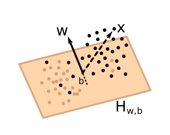
(a) Classifier view.

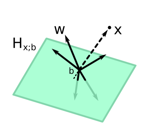
(b) Encoder view.

Figure 1: Visualizing the half-spaces associated with data point ${\bf x}$ and feature vector ${\bf w}$. In a linear classifier (left), weight vectors define hyperplanes that split data points into two groups. In a linear encoder (right), a data point ${\bf x}$ defines a hyperplane which is shifted in the direction opposite that data point through a distance $b$ associated with feature ${\bf w}$; the hidden unit corresponding to ${\bf w}$ is coded by the distance from ${\bf w}$ to the shifted hyperplane.

Many researchers (e.g., [7, 11, 5]) have described how the rectified linear activation function separates its inputs into two natural groups of outputs: those with 0 values, and those with positive values. We belabor this observation here to make a further point about the behavior of rectified linear autoencoders below.

Consider a data point ${\bf x}$ and each encoding feature (row) ${\bf w}_{j}$ of $D^{T}$ geometrically as vectors in $\mathbb{R}^{n}$, shown in Figure 1. In the context of a linear classifier, the weight vector ${\bf w}$ is often described as defining the normal to a hyperplane $H_{\bf w}$ that divides the dataset into two subsets. A linear encoder, on the other hand, is attempting to determine which hidden units describe its input, so in this context it is the vector ${\bf x}$ that defines the normal to a hyperplane $H_{\bf x}$ passing through the origin. Each feature ${\bf w}_{j}$ in the autoencoder corresponds to a bias term $b_{j}$; this bias can be seen as translating $H_{\bf x}$ in the direction away from ${\bf x}$ through a distance of $b_{j}$. After this translation, if ${\bf w}_{j}$ lies on the opposite side of $H_{{\bf x};{\bf w}_{j},b_{j}}$ from ${\bf x}$, then the hidden unit $h_{j}$ will be set to 0 by a rectified activation function. In other words, rectification selectively deactivates features ${\bf w}_{j}$ in the loss for ${\bf x}$ whenever feature ${\bf w}_{j}$ points sufficiently far away from ${\bf x}$. After hidden unit $h_{j}$ is deactivated, decoding entry ${\bf w}_{j}$ no longer has any effect on the output. We can thus define

$$\psi_{\bf x}=\left\{j:{\bf w}_{j}{\bf x}+b_{j}>0\right\}$$

as the set of features that have nonzero activations in the hidden layer of the autoencoder for input ${\bf x}$. Then

$${\bf h}_{\psi}=\left[h_{\psi_{1}},\dots,h_{\psi_{r}}\right]^{T}$$

is the vector of hidden activations for just the features in $\psi$, $D_{\psi}$ is the matrix of corresponding columns from $D$, and ${\bf b}_{\psi}$ are the corresponding bias terms. This gives a new loss function

$$\ell_{\psi}(\mathcal{O})=\frac{1}{2\left|\mathcal{O}\right|}\sum_{{\bf x}\in\mathcal{O}}\left\|D_{\psi}\left(D^{T}_{\psi}{\bf x}+{\bf b}_{\psi}\right)-{\bf x}\right\|_{2}^{2}+R(\mathcal{O},D,{\bf b})$$

that is computed only over the active features $\psi_{\bf x}$ for each input ${\bf x}$.

With ${\bf b}={\bf 0}$ and a sparse regularizer $R=\|{\bf h}\|_{1}$, the loss $\ell_{\psi}$ reduces to that proposed by Le et al. [9] for ICA with a reconstruction cost. For whitened input, then, the rectified linear autoencoder behaves not only like a mixture of exponentially many linear models [11], but rather like a mixture of exponentially many ICA models—one ICA model is selected for each input ${\bf x}$, but all features are selected from, and must coexist in, one large feature set. Importantly, this whitening requirement only holds for the region of data delimited by the set of active features, potentially simplifying the whitening transform.

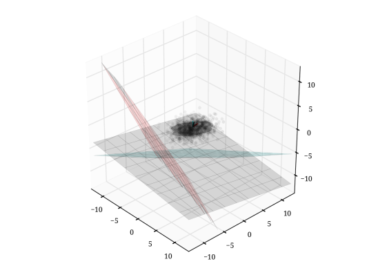
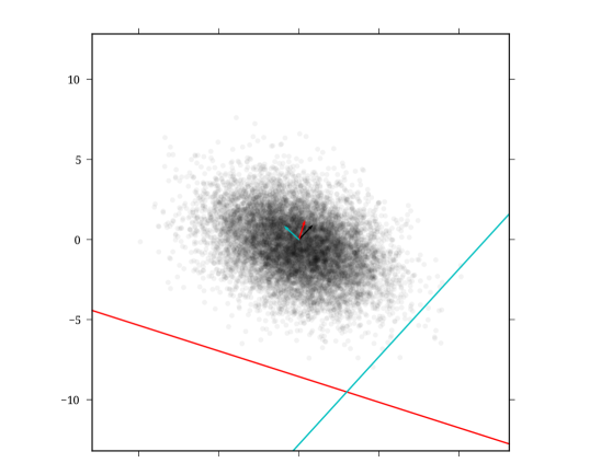
Figure 2: Rectified linear feature planes for a 3D gaussian dataset, using a complete dictionary ($k=3$). With an undercomplete or $1\times$ complete dictionary, these planes tend to move to the bounds of the dataset, forming a new coordinate system. The image on the left is a full 3D view of the space, while the image on the right is a projection onto the $x$–$y$ plane.

Mirrored by the geometric interpretation, from the perspective of a data point, nonzero bias terms can be thought of as translating the data to a new origin along the axis of that feature. Seen from the perspective of a feature, the bias terms can help move the active region for that feature to an area of space where data are available to describe—potentially ignoring other regions of space that contain other portions of the data. From either viewpoint, the bias parameters in the model can thus help compensate for non-centered data. Figure 2 shows typical behavior for a $1\times$ complete dictionary of rectified linear units when trained on an artificial 3D gaussian dataset. In this case, each feature plane uses its associated bias to translate away from the origin, together providing a sort of “bounding box” for the data. Though the axes of the box are not necessarily orthogonal, the features define a new basis that is often aligned with or near the principal axes of the data.

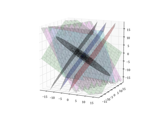
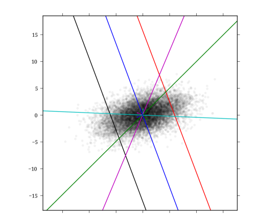
Figure 3: Sigmoid feature planes for a 3D gaussian dataset, using an overcomplete dictionary ($k=6$). The weights corresponding to each hidden neuron form the normal vector to each plane, and the distance from the origin is given by the bias for that unit. In the above example, three of the encoding planes have partitioned the major axis of the data distribution (perhaps to maximize effective coding regions), while the remaining planes capture variance along minor axes of the dataset. The image on the left is a full 3D view of the space, while the image on the right is a projection onto the $x$–$y$ plane.

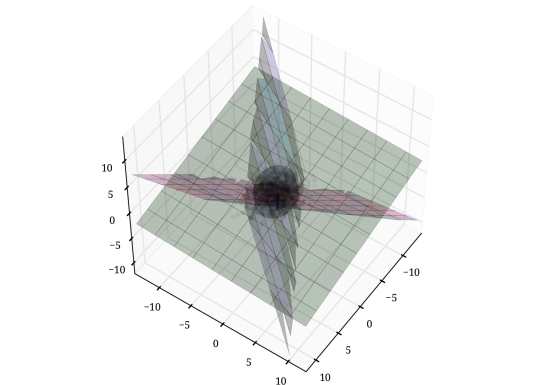
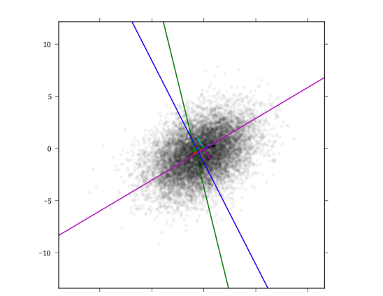
Figure 4: Rectified linear feature planes for a 3D gaussian dataset, using an overcomplete dictionary ($k=6$). These feature planes group together in pairs, splitting the dataset along one axis. The image on the left is a full 3D view of the space, while the image on the right is a projection onto the $x$–$y$ plane.

3.1 Effective coding region

Visualizing feature hyperplanes is actually instructive for many types of activation functions. Figure 3, for instance, shows the feature planes for a $2\times$ overcomplete tied-weights autoencoder with sigmoid hidden units, trained on an artificial 3D gaussian dataset. Several of the features learned by this model partition the data along the principal axis of variance, while the remaining features capture some of the variance along minor axes of the dataset. In comparison, a $2\times$ overcomplete rectified linear autoencoder trained on a 3D gaussian dataset (Figure 4) creates pairs of negated feature vectors, in effect providing a full-wave rectified linear output along each axis. Together, these pairs of planes split the data into orthants, which produces a coding scheme that is 50 % sparse because only half of the features are active for any given region of the input space.

Clearly these two activation functions have different ways of modeling the input data, but why do these particular patterns of organization appear? In our view, the unbounded linear output of the rectified linear autoencoder units addresses a subtle but important issue inherent in coding with sigmoid activation functions: scale. Consider, for example, a two-dimensional dataset consisting of points along a one-dimensional manifold

$$\mathcal{L}=\left\{[x,\epsilon]^{T}:0<x<S\right\}$$

where $\epsilon$ is gaussian noise. Regardless of the activation function, this network requires just one hidden unit to represent points in $\mathcal{L}$: we can set the bias to $0$ and weights to $[1,0]^{T}$ to align the feature of the hidden unit with the linear function that describes the data. Then points in the dataset are simply coded by their distance from the origin, as given by the output of the activation function. For a sigmoid activation function, however, as $S$ increases, the activation function saturates, limiting the power of the hidden units to discriminate between small changes in $x$ near $S$. This saturation limits the scale at which sigmoid units can describe data effectively, but it also prevents numerical instability by limiting the range of the output.

Regardless of the activation function, then, each feature vector can be seen as normal to a hyperplane in input space. The activation function encodes data along the axis of the feature as a function of the distance to the hyperplane for that feature. Sigmoid activation functions saturate for points far from the hyperplane, whereas linear activations solve this “vanishing signal” problem by coding all $x$ values with a linear output response. Rectified linear activations make a further distinction by coding only one half of the input space. However, the outputs of a linear activation are unbounded, so networks with inputs at large scales are prone to numerical instability during training.

4 Behavior on complex data

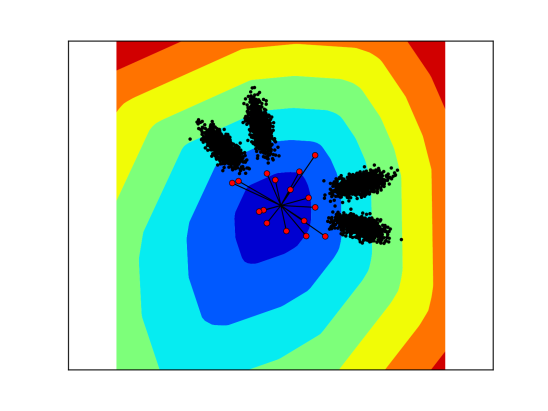
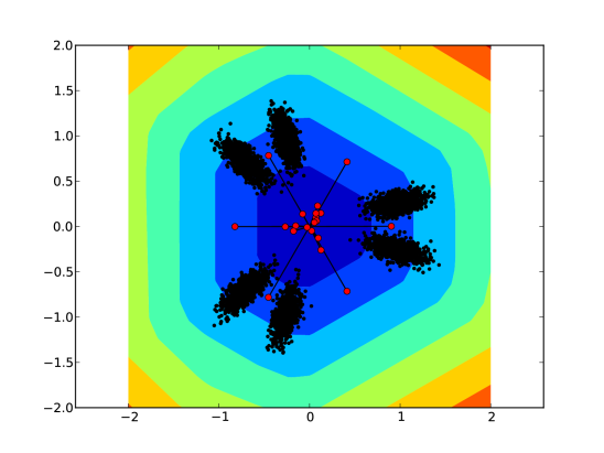
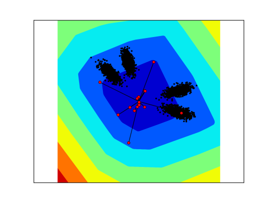
Figure 5: Rectified linear responses summed over input space for mixture of gaussian datasets. The plot on the left was trained with no regularization, while the plots in the middle and on the right were trained with an L1 sparsity penalty on the hidden activations. Color delineates regions of equal potential summed over all hidden units, and small red circles indicate the learned feature vectors. Data points are shown in black.

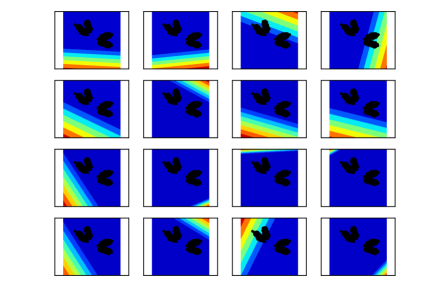
Figure 6: Summary plots of individual feature response regions for a rectified linear autoencoder trained on a mixture of gaussians dataset, including an L1 sparsity penalty. Colored bands indicate equipotential regions of response for the feature, and data points are shown in black. Interestingly, most of the features are inactive for this dataset, with only three features devoted to coding important regions of the data.

So far, the visualizations tools that we have used are based on simple gaussian distributions of data. Many interesting datasets, however, are emphatically not gaussian—indeed, one of the primary reasons that ICA is so effective is that it explicitly searches for a non-gaussian model of the data! In this section we present several visualizations for these models using more complex datasets: first we examine mixtures of gaussians, and then we use the MNIST digits dataset as a foray into a more natural set of data.

We first tested the behavior of rectified linear autoencoders on a small, 2D mixture of gaussians dataset. (See Figure 5.) After training, even massively overcomplete dictionaries tended to display the feature pairing behavior described above, particularly when combined with a sparse regularizer, suggesting that these networks are capable of identifying the number of features required to code the data effectively. Unfortunately, while it provides simple visualization, working in 2D does not necessarily generalize to higher dimensions, as our intuition in low-dimensional spaces can quickly lead us astray in larger spaces.

4.1 MNIST digits

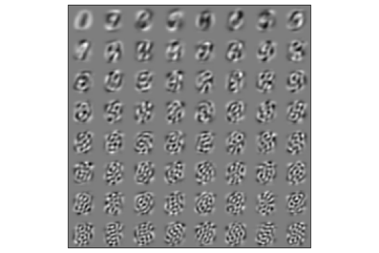
Figure 7: PCA features (eigendigits) computed for MNIST digits.

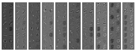
Figure 8: Some of the features computed using a single-layer rectified linear autoencoder with a $1.5\times$ overcomplete dictionary. Each feature ${\bf w}$ is displayed on the left, and on the right is its corresponding maximally negative feature ${\bf v}=\operatorname*{arg\,min}_{\bf u}{\bf w}^{T}{\bf u}$.

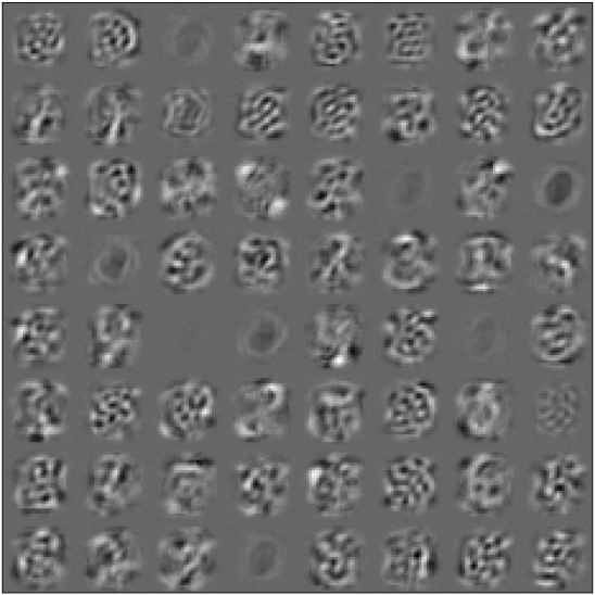
(a) 64 first-layer features.

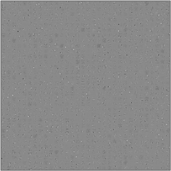
(b) 1024 second-layer features.

Figure 9: MNIST features computed using a two-layer rectified linear autoencoder.

The MNIST dataset consists of 60000 $28\times 28$ grayscale images of the handwritten digits 0 through 9. Figure 7 shows the PCA “eigendigits” computed using this dataset; these digits point in the directions of highest variance for this dataset overall, and are often interpreted as a coding of the digit using a Fourier basis. Figure 8 shows the features with the highest bias values computed by a single-layer rectified linear autoencoder on the same dataset. For visualization purposes, each feature ${\bf w}$ on the left of each column is paired with its maximally negative feature ${\bf v}=\operatorname*{arg\,min}_{\bf u}{\bf w}^{T}{\bf u}$ from the dictionary. Many of the primary features in the dictionary are negative images of each other, indicating that the “pairing” of feature planes observed for low-dimensional datasets also occurs with higher-dimensional data.

Finally, Figure 9 shows features learned by a two-layer rectified linear autoencoder with untied weights. This model was trained with just 64 first-layer hidden units, and 1024 second-layer units. As observed in the low-dimensional gaussian data, the features from the first layer appear to model the principal axes of the data, providing a bounding box of 64 dimensions that encodes the data for the next layer. The features from the second layer resemble a more traditional sparse code, consisting in this case of small segments of pen strokes. It is important to note that the training dataset was not whitened beforehand, and no regularization was used to train the network—the autoencoder learned these features automatically, using only a squared error reconstruction cost.

5 Conclusion

This paper has synthesized many recent developments in encoding and neural networks, with a focus on rectified linear activation functions and whitening. It also presented an intuitive interpretation for the behavior of these encodings through simple visualizations. Sample features learned from both artificial and natural datasets provided examples of learning behavior when these algorithms are applied to different types of data.

There are many more paths to explore in this area of machine learning research. Whitening has appeared in many places throughout this paper and seems to be a very important component of linear autoencoders and coding systems in general. However, this connection seems poorly understood, and would benefit from further exploration, particularly with respect to the idea of whitening local regions of the input space.

References

- [1] A. Coates, H. Lee, and A.Y. Ng. An analysis of single-layer networks in unsupervised feature learning. In AISTATS, volume 1001, page 48109, 2011.
- [2] A. Coates and A.Y. Ng. The importance of encoding versus training with sparse coding and vector quantization. In International Conference on Machine Learning, volume 8, page 10, 2011.
- [3] Y. Dan, J.J. Atick, and R.C. Reid. Efficient coding of natural scenes in the lateral geniculate nucleus: experimental test of a computational theory. The Journal of Neuroscience, 16(10):3351–3362, 1996.
- [4] M. Denil and N. de Freitas. Recklessly approximate sparse coding, 2012.
- [5] X. Glorot, A. Bordes, and Y. Bengio. Deep sparse rectifier neural networks. In Proceedings of the Fourteenth International Conference on Artificial Intelligence and Statistics (AISTATS 2011), 2011.
- [6] K Gregor and Y LeCun. Learning fast approximations of sparse coding. In Proc. International Conference on Machine learning (ICML’10), 2010.
- [7] R.H.R. Hahnloser, H.S. Seung, and J.J. Slotine. Permitted and forbidden sets in symmetric threshold-linear networks. Neural Computation, 15(3):621–638, 2003.
- [8] G.E. Hinton and R.S. Zemel. Autoencoders, minimum description length, and Helmholtz free energy. Advances in Neural Information Processing Systems, pages 3–3, 1994.
- [9] Q.V. Le, A. Karpenko, J. Ngiam, and A.Y. Ng. ICA with reconstruction cost for efficient overcomplete feature learning. In Advances in Neural Information Processing Systems, 2011.
- [10] A. Lemme, R.F. Reinhart, and J.J. Steil. Efficient online learning of a non-negative sparse autoencoder. In Proceedings of the ESANN, pages 1–6, 2010.
- [11] V. Nair and G.E. Hinton. Rectified linear units improve restricted boltzmann machines. In 27th International Conference on Machine Learning, pages 807–814. Omnipress Madison, WI, 2010.
- [12] B.A. Olshausen and D.J. Field. Emergence of simple-cell receptive field properties by learning a sparse code for natural images. Nature, 381(6583):607–609, 1996.
- [13] E.P. Simoncelli and B.A. Olshausen. Natural image statistics and neural representation. Annual review of neuroscience, 24(1):1193–1216, 2001.
- [14] R. Tibshirani. Regression shrinkage and selection via the lasso. Journal of the Royal Statistical Society. Series B (Methodological), pages 267–288, 1996.
- [15] P. Vincent, H. Larochelle, Y. Bengio, and P.A. Manzagol. Extracting and composing robust features with denoising autoencoders. In Proceedings of the 25th international conference on Machine learning, pages 1096–1103. ACM, 2008.