Conformal deformations of immersed discs in $\mathbb{R}^{3}$ and elliptic boundary value problems

Abstract.

Boundary value problems for operators of Dirac type arise naturally in connection with the conformal geometry of surfaces immersed in Euclidean 3–space. Recently such boundary value problems have been successfully applied to a variety of problems from computer graphics. Here we investigate under which conditions these boundary value problems are elliptic and self–adjoint. We show that under certain periodic deformations of the boundary data our operators exhibit non-trivial spectral flow.

1. Introduction

An elliptic operator on a compact manifold $M$ without boundary can be extended to a Fredholm operator between appropriate Sobolev spaces. If in addition the operator is formally self–adjoint, this extension is self–adjoint. As a consequence, the spectrum is then real and discrete and there exists a basis of eigenvectors. On compact manifolds with boundary the situation is essentially the same if one imposes boundary conditions that are elliptic and self–adjoint. This paper investigates the conditions for ellipticity and self–adjointness of certain local boundary value problems that arise in surface theory and computer graphics.

The elliptic operators we deal with are operators of Dirac type that allow to describe conformal deformations of immersed surfaces in Euclidean 3–space. They can be most easily described within the quaternionic approach [10] of G. Kamberov, F. Pedit, and the second author (see also [12, 18] for different perspectives on the application of Dirac operators to surface theory). Given an immersion $f\colon M\rightarrow\mathbb{R}^{3}=\operatorname{Im}(\mathbb{H})$ into Euclidean 3–space viewed as the imaginary quaternions, every conformal deformation $\tilde{f}$ of $f$ has a differential of the form

$$d\tilde{f}=\bar{\lambda}df\lambda,$$

where $\lambda\colon M\rightarrow\mathbb{H}_{*}$ is a quaternion valued function satisfying a Dirac type equation

(1.1) $$\mathcal{D}\lambda=\rho\lambda$$

for some real valued function $\rho$ with $\mathcal{D}$ an elliptic operator attached to $f$. By conformal deformation we mean here an immersion $\tilde{f}$ that induces the same conformal structure as the original immersion $f$ and is topologically equivalent to $f$ (i.e., in the same regular homotopy class).

In [7] it is shown that this relation between surface theory and Dirac operators can be turned into an efficient method for implementing conformal deformations in computer graphics. The idea of [7] is to “reverse” the above correspondence that assigns to a conformal deformation $\tilde{f}$ of $f$ the Dirac potential $\rho$ in (1.1) and to describe conformal deformations $\tilde{f}$ of a given immersion $f$ by the corresponding potentials $\rho$. This makes sense, because by the above every conformal deformation $\tilde{f}$ of a given $f$ can indeed be obtained from a suitable real function $\rho$ by solving for $\lambda$ in the kernel of $\mathcal{D}-\rho$ and integrating $d\tilde{f}=\bar{\lambda}df\lambda$.

The main difficulty with this idea (apart from controlling the periods of $d\tilde{f}=\bar{\lambda}df\lambda$ if $M$ has non–trivial topology) is that the correspondence between $\rho$ and $\tilde{f}$ is not a bijection. For example, given a real function $\rho$, the operator $\mathcal{D}-\rho$ might not have a kernel; and if it has one, the kernel might not be 1–dimensional and sections in the kernel might have zeros, so that $\tilde{f}$ is not immersed. As shown in [7], the first issue (that $\operatorname{ker}(\mathcal{D}-\rho)$ might be empty) can be efficiently dealt with by allowing to modify $\rho$ by a real constant $\sigma$, that is, by taking for $\lambda$ an eigenspinor

$$(\mathcal{D}-\rho)\lambda=\sigma\lambda$$

with $\sigma$ an eigenvalue of preferably small modulus (the second issue can be ignored for many applications in computer graphics, because generically a non–trivial eigenspace will be 1–dimensional). For the method of [7] to work it is crucial to make sure that the spectrum of $\mathcal{D}-\rho$ is (or at least contains) a non–empty real point spectrum. This is always the case if the underlying surface $M$ is compact and has no boundary. For a compact surface $M$ with boundary this is still the case if one imposes elliptic and self–adjoint boundary conditions.

This paper derives and discusses geometric conditions for the ellipticity and self–adjointness of local boundary conditions (i.e., pointwise conditions on the restriction $\lambda_{|\partial M}$ of the spinor $\lambda$ to the boundary) for Dirac operators induced by immersions of compact surfaces with boundary. This kind of boundary conditions seems to be most relevant for applications in computer graphics.

In Section 2 we give a brief, but self–contained review of the quaternionic approach to Dirac type operators that arise in the context of surface theory in Euclidean 3–space. In Section 3 we geometrically characterize the ellipticity and self–adjointness of local boundary conditions for such Dirac type operators. In Section 4 we compute the Fredholm index of elliptic local boundary conditions in the case that the underlying surface is a disc. Such boundary conditions turn out to be homotopy equivalent to problems studied by Vekua in the early days of index theory. In Section 5 we compute the spectral flow in the case of periodic families of self–adjoint, elliptic local boundary conditions for conformal immersions of the disc. In Section 6 we conclude the paper by describing a relation between spectral flow and the Dirac spectrum of the round 2–sphere $S^{2}$.

2. Conformal deformations and the Dirac operator $\mathcal{D}$ attached to surfaces immersed in Euclidean 3–space

Conformal deformations of surfaces in Euclidean 3–space can be efficiently described [7] in terms of quaternions and Dirac type operators. The underlying quaternionic approach to surface theory in Euclidean 3–space was first described in [10], a related but more abstract setting is developed in [12, 8, 6].

The quaternions are the 4–dimensional real vector space

$$\mathbb{H}=\mathbb{R}\oplus\mathbb{R}i\oplus\mathbb{R}j\oplus\mathbb{R}k$$

with multiplication satisfying $ij=-ji=k$ and $i^{2}=j^{2}=-1$. The first summand of a quaternion $x\in\mathbb{H}$ is called its real part $\operatorname{Re}(x)$, the $ijk$–summands together are called its imaginary part $\operatorname{Im}(x)$. The conjugation of a quaternion $x\in\mathbb{H}$ is

$$\bar{x}=\operatorname{Re}(x)-\operatorname{Im}(x).$$

The Euclidean scalar product on $\mathbb{H}=\mathbb{R}^{4}$ can be written as

$$\langle x,y\rangle_{\mathbb{R}^{4}}=\operatorname{Re}(\bar{x}y).$$

In particular, the length of a quaternion is $|x|=\sqrt{\bar{x}x}$. The imaginary quaternions $\operatorname{Im}(\mathbb{H})=\mathbb{R}^{3}$ serve as our model of Euclidean 3–space. The quaternion product

(2.1) $$xy=-\langle x,y\rangle_{\mathbb{R}^{3}}+x\times y$$

of $x$, $y\in\operatorname{Im}(\mathbb{H})=\mathbb{R}^{3}$ encodes both the scalar product $\langle x,y\rangle_{\mathbb{R}^{3}}$ and cross product $x\times y$. For $\lambda\in\mathbb{H}_{*}=\mathbb{H}\backslash\{0\}$ we define $\Phi_{\lambda}(x):=\bar{\lambda}x\lambda$. Then $\Phi_{\lambda}$ is an orientation preserving similarity of $\mathbb{R}^{3}=\operatorname{Im}(\mathbb{H})$, i.e., the product of an isometry and a homothety, and all orientation preserving linear similarities of $\mathbb{R}^{3}$ arise this way for $\lambda\in\mathbb{H}_{*}$ unique up to sign. In particular, $Spin(3)\cong S^{3}=\{x\in\mathbb{H}\mid|x|=1\}$.

Throughout the paper we denote by $M$ a compact, oriented surface with possibly non–empty boundary. We call two immersions $\tilde{f}$, $f\colon M\rightarrow\mathbb{R}^{3}=\operatorname{Im}(\mathbb{H})$ of $M$ topologically equivalent if they belong to the same regular homotopy class. (If $M$ is simply connected, then any two immersions are topologically equivalent; otherwise two immersions are topologically equivalent if and only if they induce the same spin structure [14]). We call an immersion $\tilde{f}\colon M\rightarrow\mathbb{R}^{3}=\operatorname{Im}(\mathbb{H})$ a conformal deformation of an immersion $f\colon M\rightarrow\mathbb{R}^{3}=\operatorname{Im}(\mathbb{H})$ if $\tilde{f}$ and $f$ are topologically equivalent and induce the same conformal structure on $M$. The following proposition says how conformal deformations can be described in terms of Dirac operators.

Proposition 1 (Kamberov, Pedit, and Pinkall [10]).

Let $\tilde{f}$, $f\colon M\rightarrow\mathbb{R}^{3}=\operatorname{Im}(\mathbb{H})$ be two immersions of an oriented surface $M$ that are topologically equivalent. Then $\tilde{f}$ is conformal to $f$ if and only if there exists $\lambda\colon M\rightarrow\mathbb{H}_{*}$ such that

$$d\tilde{f}=\bar{\lambda}df\lambda.$$

Conversely, given an immersion $f\colon M\rightarrow\mathbb{R}^{3}=\operatorname{Im}(\mathbb{H})$ and $\lambda\colon M\rightarrow\mathbb{H}_{*}$, the 1–form $d\tilde{f}=\bar{\lambda}df\lambda$ is closed if and only if

(2.2) $$df\wedge d\lambda=-\rho\lambda|df|^{2},$$

where $|df|^{2}$ denotes the area form induced by $f$ and $\rho$ is a real valued function on $M$.

Proof.

Two immersions $\tilde{f}$, $f\colon M\rightarrow\mathbb{R}^{3}=\operatorname{Im}(\mathbb{H})$ induce the same conformal structure if and only if locally there exists $\lambda$ with $d\tilde{f}=\bar{\lambda}df\lambda$. The global existence of $\lambda$ is then equivalent to the fact that $f$ and $\tilde{f}$ induce the same spin structure (and therefore, according to the above terminology, are topologically equivalent and hence conformal deformations of each other). The integrability condition takes the form (2.2), because

$$0=d(\bar{\lambda}df\lambda)=-\operatorname{Im}(\bar{\lambda}df\wedge d\lambda)$$

is equivalent to $\bar{\lambda}df\wedge d\lambda=\rho|\lambda|^{2}|df|^{2}$ with $\rho$ a real function. ∎

For an immersion $f\colon M\rightarrow\mathbb{R}^{3}=\operatorname{Im}(\mathbb{H})$ of an oriented surface $M$ we define

(2.3) $$\mathcal{D}\lambda=-\frac{df\wedge d\lambda}{|df|^{2}}$$

with $|df|^{2}$ denoting the area form induced by $f$. The quaternionic linear operator

$$\mathcal{D}\colon C^{\infty}(M,\mathbb{H})\rightarrow C^{\infty}(M,\mathbb{H})$$

is formally self–adjoint and elliptic. In Subsection 3.3 below it is shown that $\mathcal{D}$ is a Dirac type operator. We therefore refer to $\mathcal{D}$ as the Dirac operator induced by the immersion $f$.

Using the Dirac operator $\mathcal{D}$, the integrability equation (2.2) can be rewritten as

(2.4) $$\mathcal{D}\lambda=\rho\lambda.$$

As shown in [10], the potential $\rho$ measures the difference

(2.5) $$\tilde{H}|d\tilde{f}|=H|df|+\rho|df|$$

between the mean curvature half–densities $\tilde{H}|d\tilde{f}|$ of $\tilde{f}$ and $H|df|$ of $f$, where for the mean curvature we take the definition $H=\frac{1}{2}\operatorname{tr}\langle df,dN\rangle$ so that $H=1$ for the unit sphere with the orientation such that the outside normal is positive. The mean curvature half–density is the square root of the Willmore integrand.

As explained in the introduction, for the application of the computer graphics algorithm proposed in [7] one wants $\mathcal{D}-\rho$ to have a non–empty real point spectrum. If the underlying compact surface $M$ has a non–empty boundary, this can be guaranteed by posing elliptic and self–adjoint boundary conditions. In the next section we geometrically characterize the ellipticity and self–adjointness of local boundary conditions for $\mathcal{D}$, i.e., boundary conditions given by orientable subbundles $E^{\prime}$ of the trivial $\mathbb{H}$–bundle over $\partial M$ that prescribe the values admissible for the restriction $\lambda_{|\partial M}$ of $\lambda$. As it turns out, the relevant local boundary conditions are given by real two–dimensional bundles $E^{\prime}$.

In the remainder of the section we discuss the geometry behind and examples of the local boundary conditions for $\mathcal{D}$ given by real two–dimensional, orientable subbundles $E^{\prime}$ of the trivial $\mathbb{H}$–bundle. We use that every real two–dimensional plane $E^{\prime}$ in $\mathbb{H}$ is of the form

(2.6) $$E^{\prime}=\{\lambda\in\mathbb{H}\mid V\lambda=\lambda\tilde{V}\}$$

with $V$, $\tilde{V}\in S^{2}$ unique up to a common $\mathbb{Z}_{2}$–factor, see [6, Lemma 2]. A real two–dimensional, orientable subbundle $E^{\prime}$ of the trivial $\mathbb{H}$–bundle over $\partial M$ thus corresponds to a pair of smooth maps $V$, $\tilde{V}\colon\partial M\rightarrow S^{2}$ which is unique up to a common $\mathbb{Z}_{2}$–factor (a non–orientable $E^{\prime}$ would correspond to $V$, $\tilde{V}$ with $\mathbb{Z}_{2}$–monodromy along the boundary). A nowhere vanishing spinor $\lambda$ satisfies the boundary condition given by $E^{\prime}$ if and only if

$$\tilde{V}=\lambda^{-1}V\lambda\qquad\textrm{ along }\qquad\partial M.$$

This condition can be best understood through the examples provided by the canonical boundary conditions discussed in the following.

An immersion $f\colon M\rightarrow\mathbb{R}^{3}=\operatorname{Im}(\mathbb{H})$ of a compact, oriented surface $M$ with a non–empty boundary $\partial M$ is equipped with a canonical frame $(T,N,B)$ along $\partial M$, where $N$ is the Gauss–map, $T$ the positive unit tangent vector field along the boundary, and $B=T\times N$ its bi–normal field. Let $\tilde{f}$ be a conformal deformation of $f$ given by $d\tilde{f}=\bar{\lambda}df\lambda$ with $\lambda$ a nowhere vanishing solution to $\mathcal{D}\lambda=\rho\lambda$ for $\mathcal{D}$ the Dirac operator induced by $f$ and $\rho$ a real valued function. Then, the canonical frame along the boundary of $\tilde{f}$ is given by

$$\tilde{T}=\lambda^{-1}T\lambda,\qquad\tilde{N}=\lambda^{-1}N\lambda,\qquad\textrm{ and }\qquad\tilde{B}=\lambda^{-1}B\lambda.$$

The canonical frame $(T,N,B)$ gives rise to three types of canonical boundary conditions, the boundary conditions obtained by choosing $V=T$, $V=N$, or $V=B$, respectively. Denoting the second vector field $\tilde{V}$ in (2.6) by $\tilde{V}=\tilde{T}$, $\tilde{V}=\tilde{N}$, or $\tilde{V}=\tilde{B}$, respectively, the geometric meaning of the local boundary condition given by $(V,\tilde{V})$ becomes

$$V=T,\qquad \tilde{V}=\tilde{T} \quad\leadsto\qquad \tilde{f}\textrm{ has prescribed }\tilde{T}=\lambda^{-1}T\lambda,or$$

$$V=N,\qquad \tilde{V}=\tilde{N} \quad\leadsto\qquad \tilde{f}\textrm{ has prescribed }\tilde{N}=\lambda^{-1}N\lambda,or$$

$$V=B,\qquad \tilde{V}=\tilde{B} \quad\leadsto\qquad \tilde{f}\textrm{ has prescribed }\tilde{B}=\lambda^{-1}B\lambda,$$

respectively.

3. Elliptic and self–adjoint local boundary conditions for $\mathcal{D}$

We derive geometric conditions characterizing the ellipticity and self–adjointness of local boundary conditions for the Dirac operator $\mathcal{D}$ attached to immersions $f\colon M\rightarrow\mathbb{R}^{3}=\operatorname{Im}(\mathbb{H})$ of oriented surfaces $M$ with boundary. Imposing elliptic and self–adjoint boundary conditions for the Dirac operator $\mathcal{D}$ assures that $\mathcal{D}-\rho$ with $\rho$ a real function behaves essentially as in the case of compact surfaces without boundary (cf. Subsection 3.6).

3.1. Conditions for ellipticity and self–adjointness of local boundary conditions

By a local boundary condition for the Dirac operator $\mathcal{D}$ in (2.3) we mean a smooth, orientable real subbundle $E^{\prime}$ of the trivial $\mathbb{H}$–bundle over $\partial M$ that prescribes the admissible values of the restriction $\lambda_{|\partial M}$ of $\lambda$ to the boundary $\partial M$. (The assumption that $E^{\prime}$ is orientable is included to simplify the notation; Theorems 1 and 2 below hold also in the non–orientable case, although the vector fields $V$ and $\tilde{V}$ then have $\mathbb{Z}_{2}$–monodromy.)

The following two theorems imply that elliptic or self–adjoint local boundary conditions are necessarily given by two–dimensional subbundles $E^{\prime}$. As explained in Section 2, every real two–dimensional, orientable subbundle $E^{\prime}$ of the trivial $\mathbb{H}$–bundle over $\partial M$ is given by a pair of vector fields $V$, $\tilde{V}\colon\partial M\rightarrow S^{2}\subset\operatorname{Im}(\mathbb{H})$ along $\partial M$ for which

(3.1) $$E^{\prime}_{p}=\{\lambda\in\mathbb{H}\mid V(p)\lambda=\lambda\tilde{V}(p)\}.$$

Theorem 1.

Let $f\colon M\rightarrow\mathbb{R}^{3}=\operatorname{Im}(\mathbb{H})$ be a conformal immersion of a compact Riemann surface $M$ with boundary. A local boundary condition $E^{\prime}$ for the Dirac operator (2.3) induced by $f$ is elliptic if and only if $E^{\prime}$ is a two–dimensional real orientable vector bundle such that the corresponding maps $V$, $\tilde{V}\colon\partial M\rightarrow S^{2}\subset\operatorname{Im}(\mathbb{H})$ satisfy

$$V(p)\neq\pm N(p)\qquad\textrm{for all}\quad p\in\partial M,$$

where $N$ is the Gauss map $N\colon M\rightarrow S^{2}$ of $f$.

Theorem 2.

Let $f\colon M\rightarrow\mathbb{R}^{3}=\operatorname{Im}(\mathbb{H})$ be a conformal immersion of a compact Riemann surface $M$ with boundary. A local boundary condition $E^{\prime}$ for the Dirac operator (2.3) induced by $f$ is self–adjoint if and only if $E^{\prime}$ is a two–dimensional real orientable vector bundle such that the corresponding maps $V$, $\tilde{V}\colon\partial M\rightarrow S^{2}\subset\operatorname{Im}(\mathbb{H})$ satisfy

$$V(p)\perp T(p)\qquad\textrm{for all}\quad p\in\partial M,$$

where $T$ denotes the positive unit tangent field of $f$ along the boundary $\partial M$ of $M$.

As an immediate consequence of Theorems 1 and 2 we obtain for the three canonical boundary conditions (see the end of Section 2) that

• the bi–normal boundary condition which prescribes $\tilde{B}$ is elliptic and self–adjoint,

• the tangential boundary condition which prescribes $\tilde{T}$ is elliptic, but not self–adjoint, and

• the normal boundary condition which prescribes $\tilde{N}$ is self–adjoint, but not elliptic.

The proofs of Theorems 1 and 2 are given in 3.4 and 3.5 below. In order to make them more accessible to Readers not familiar with elliptic boundary value problems, we give detailed references to the excellent, self–contained text [2] by C. Bär and W. Ballmann on first order elliptic boundary value problems. In particular, in 3.2 we review the necessary notation of [2] and in 3.3 we explain that we are in the “standard setup” of [2]. We follow the notation of [2] with two notable differences:

• In the following analysis all linear operators, even if they are quaternionic linear, are viewed as real instead of complex linear operators; in other words, the complex structure obtained by restriction to the complex scalar field is not used. This might seem confusing at first thought, but is geometrically necessary if one wants to allow for real subbundles $E^{\prime}$ as boundary conditions. (At the only point where we actually need the complex scalar field, we simply complexify the whole setup, cf. the proof of Theorem 1 in Section 3.4.)

• In contrast to [2] we are exclusively interested in the case that $M$ is compact with boundary and apply corresponding simplifications of the notation. In particular, we denote by $C^{\infty}(M,E)$ the space of smooth section of $M$ and by $C^{\infty}_{0}(M,E)$ the space of smooth sections with support in $M\backslash\partial M$ (for which [2] would instead write $C^{\infty}_{c}(M,E)$ and $C^{\infty}_{cc}(M,E)$, respectively).

3.2. General theory of local boundary conditions for first order elliptic operators (following [2])

Let $\mathcal{D}\colon C^{\infty}(M,E)\rightarrow C^{\infty}(M,F)$ be a first order elliptic operator as in the standard setup 1.5 of [2]. We view $\mathcal{D}$ as a densely defined unbounded operator $\mathcal{D}_{0}$ with domain $\operatorname{dom}(\mathcal{D}_{0})=C^{\infty}_{0}(M,E)$ in $L^{2}(M,E)$. In the case that $\partial M=\emptyset$ there is one distinguished extension of $\mathcal{D}_{0}$, its closure defined on the first Sobolev space. In the case $\partial M\neq\emptyset$ which we are interested in, there are many extensions of $\mathcal{D}_{0}$ corresponding to the different boundary conditions.

The so called maximal extension $\mathcal{D}_{max}$ of $\mathcal{D}_{0}$ (cf. p.4 of [2]) has as its domain $\operatorname{dom}(\mathcal{D}_{max})$ the space of all $\phi\in L^{2}(M,E)$ for which $\mathcal{D}\phi$ exists in the distribution sense and $\mathcal{D}\phi\in L^{2}(M,E)$, i.e., $\phi\in\operatorname{dom}(\mathcal{D}_{max})$ if and only if $\phi\in L^{2}(M,E)$ and there is $\xi\in L^{2}(M,F)$ such that

$$\langle\phi,\mathcal{D}^{*}\psi\rangle=\langle\xi,\psi\rangle$$

for all $\psi\in C^{\infty}_{0}(M,F)$. Here $\mathcal{D}^{*}\colon C^{\infty}(M,F)\rightarrow C^{\infty}(M,E)$ denotes the formal adjoint of $\mathcal{D}$, the operator characterized by

$$\langle\mathcal{D}\phi,\psi\rangle=\langle\phi,\mathcal{D}^{*}\psi\rangle$$

for all $\phi\in C^{\infty}_{0}(M,E)$ and $\psi\in C^{\infty}_{0}(M,F)$. More elegantly, one can characterize $\mathcal{D}_{max}$ as the adjoint $(\mathcal{D}^{*})^{ad}$ of the formal adjoint $\mathcal{D}^{*}$ in the unbounded operator sense. This immediately shows that $\mathcal{D}_{max}$ is a closed extension of $\mathcal{D}_{0}$. In particular, the graph norm makes $\operatorname{dom}(\mathcal{D}_{max})$ into a Hilbert space.

There are two equivalent ways of describing boundary conditions for $\mathcal{D}$:

1. by prescribing boundary values of sections of $E$,

2. by prescribing a closed extension of $\mathcal{D}_{0}$ contained in $\mathcal{D}_{max}$.

The first point (1) is technically more involved: by Theorem 1.7 or 6.7 in [2], the space $C^{\infty}(M,E)$ is dense in $\operatorname{dom}(\mathcal{D}_{max})$ with respect to the graph norm and the restriction map $\mathcal{R}\colon C^{\infty}(M,E)\rightarrow C^{\infty}(\partial M,E)$, $\phi\mapsto\phi_{|\partial M}$ has a unique continuous extension to $\operatorname{dom}(\mathcal{D}_{max})$ which is a surjective map to the space $\check{H}(A)$ (defined in (3) or (36) of [2]). A boundary condition can then be defined as a closed subspace $B$ of $\check{H}(A)$ (see Def. 1.9 or 7.1 of [2]). Such a boundary condition $B$ defines a closed extension $\mathcal{D}_{B,max}$ of $\mathcal{D}_{0}$ contained in $\mathcal{D}_{max}$, i.e.,

$$\mathcal{D}_{0}\subset\mathcal{D}_{B,max}\subset\mathcal{D}_{max}$$

with domain

$$\operatorname{dom}(\mathcal{D}_{B,max})=\{\phi\in\operatorname{dom}(\mathcal{D}_{max})\mid\mathcal{R}\phi\in B\},$$

see (4) or 7.1 of [2]. Conversely, by Prop. 7.2 of [2], every closed extension of $\mathcal{D}_{0}$ contained in $\mathcal{D}_{max}$ is of the form $\mathcal{D}_{B,max}$ for some boundary condition $B$, showing that boundary conditions (1) can be equivalently described by closed extensions (2). For example, the closure of $\mathcal{D}_{0}$, the so called minimal extension $\mathcal{D}_{min}$, corresponds to the Dirichlet boundary condition $B=\{0\}$.

A local boundary condition corresponding to a subbundle $E^{\prime}$ of $E$ is obtained by taking for $B$ the closure of $C^{\infty}(\partial M,E^{\prime})$ in $\check{H}(A)$ (this slightly differs from Definition 7.19 in [2], but is equivalent in the elliptic case, cf. Lemma 7.10 and the following remark in [2]). For example, $E^{\prime}=\{0\}$ and $E^{\prime}=E$ yield the minimal and maximal extensions.

The adjoint of an operator $\mathcal{D}_{B,max}$ corresponding to a boundary condition $B$ for $\mathcal{D}$ is the operator

$$(\mathcal{D}_{B,max})^{ad}=\mathcal{D}^{*}_{B^{ad},max}$$

for $B^{ad}$ the adjoint boundary condition (see Section 7.2 of [2]) given by

(3.2) $$B^{ad}=\{\psi\in\check{H}(\tilde{A})\mid\langle\sigma_{0}\varphi,\psi\rangle=0\textrm{ for all }\varphi\in B\},$$

see (6) or (63) in [2], because, by (48) there, for all $\varphi\in\operatorname{dom}(\mathcal{D}_{max})$ and $\psi\in\operatorname{dom}(\mathcal{D}^{*}_{max})$

$$\langle\mathcal{D}_{max}\varphi,\psi\rangle_{L^{2}(M)}-\langle\varphi,(\mathcal{D}^{*})_{max}\psi\rangle_{L^{2}(M)}=-\langle\sigma_{0}\mathcal{R}\varphi,\mathcal{R}\psi\rangle_{L^{2}(\partial M)}.$$

The adjoint boundary condition of the local boundary condition given by $E^{\prime}$ is again local and given by $F^{\prime}=(\sigma_{0}(E^{\prime}))^{\perp}$ (for example, the minimal and maximal boundary conditions are adjoint to each other). To see this we have to check that $B^{ad}$ is the closure of $C^{\infty}(\partial M,(\sigma_{0}(E^{\prime}))^{\perp})$. It is clear by (3.2) that the closure of $C^{\infty}(\partial M,(\sigma_{0}(E^{\prime}))^{\perp})$ is contained in $B^{ad}$. They coincide by Lemma 6.3 in [2], because under the perfect pairing $\beta$ the decomposition of the dense subspace $C^{\infty}(\partial M,E)=C^{\infty}(\partial M,E^{\prime})\oplus C^{\infty}(\partial M,(E^{\prime})^{\perp})$ of $\check{H}(A)$ induces a direct sum decomposition of the space $\check{H}(\tilde{A})$ into closed subspaces one of which is the closure of $C^{\infty}(\partial M,(\sigma_{0}(E^{\prime}))^{\perp})$.

This immediately yields a condition for the operator $\mathcal{D}_{B,max}$ corresponding to a local boundary condition to be self–adjoint. For this, the underlying differential operator $\mathcal{D}$ has to be formally self–adjoint which means that $\mathcal{D}=\mathcal{D}^{*}$ (and hence necessarily $E=F$), i.e.,

$$\langle\mathcal{D}\phi,\psi\rangle=\langle\phi,\mathcal{D}\psi\rangle$$

for all $\phi$, $\psi\in C^{\infty}_{0}(M,E)$. In the formally self–adjoint case, the adjoint boundary condition $B^{ad}$ of a given boundary condition $B$ is a boundary condition for the same differential operator $\mathcal{D}$. The extension $\mathcal{D}_{B,max}$ is then self–adjoint if and only if $B=B^{ad}$. In particular, a local boundary condition given by $E^{\prime}$ is self–adjoint if and only if

(3.3) $$E^{\prime}=(\sigma_{0}(E^{\prime}))^{\perp}.$$

Even more important than self–adjointness for what follows is the ellipticity of boundary conditions which implies the Fredholm property of the extension $\mathcal{D}_{B,max}$ (see Subsection 3.6 for references): a boundary condition is elliptic if and only if

$$\operatorname{dom}(\mathcal{D}_{B,max})\subset H^{1}_{loc}(M,E)\quad\textrm{ and }\quad\operatorname{dom}(\mathcal{D}^{*}_{B^{ad},max})\subset H^{1}_{loc}(M,F)$$

(see Definition 1.10 in [2] and also Remark 1.11 and Definition 7.5 for alternative Definitions which are equivalent by Theorems 1.12 and 7.11).

3.3. Adaption to “standard setup” described in 1.5 of [2]:

In the rest of the paper $\mathcal{D}$ is the Dirac operator (2.3) induced by an immersion $f\colon M\rightarrow\mathbb{R}^{3}=\operatorname{Im}(\mathbb{H})$ of an oriented surface $M$ with boundary. The immersion $f$ also defines a volume form on $M$ which enters into the definition of $L^{2}$– and Sobolev norms (although on a compact manifold changing the volume form yields equivalent $L^{2}$– and Sobolev norms).

To make contact with the “standard setup” [2, 1.5], we denote by $E=F$ the trivial $\mathbb{R}^{4}=\mathbb{H}$–bundle over $M$ with scalar product $\langle\lambda,\mu\rangle=\operatorname{Re}(\bar{\lambda}\mu)$ and view our Dirac operator $\mathcal{D}$ as a real linear map $\mathcal{D}\colon C^{\infty}(M,E)\rightarrow C^{\infty}(M,F)$ between smooth sections of $E=F$. The operator $\mathcal{D}$ is elliptic, because its symbol [2, (21)] is

(3.4) $$\sigma_{\mathcal{D}}(\xi)(\lambda)=-\frac{df\wedge\xi}{|df|^{2}}\lambda$$

for $\xi\in T^{*}_{p}M$ and $\lambda\in E_{p}=\mathbb{H}$ so that $\sigma_{\mathcal{D}}(\xi)$ is an isomorphism for every $\xi\neq 0$.

To see that we are in the standard setup, we check that $\mathcal{D}$ is a Dirac type operator in the sense of [2, Example 4.3(a)]. Because

$$\sigma_{\mathcal{D}}(\xi)^{*}=-\sigma_{\mathcal{D}^{*}}(\xi)$$

(see [2, (22)]) and $\mathcal{D}$ is formally self–adjoint, $\mathcal{D}=\mathcal{D}^{*}$, the condition that $\mathcal{D}$ is a Dirac type operator reads

$$\sigma_{\mathcal{D}}(\xi)\sigma_{\mathcal{D}}(\eta)+\sigma_{\mathcal{D}}(\eta)\sigma_{\mathcal{D}}(\xi)=-2\langle\xi,\eta\rangle\operatorname{Id}_{E}$$

for all $\xi$, $\eta\in T^{*}_{p}M$ and $p\in M$. This condition can be easily verified, e.g. by taking $\xi$, $\eta\in\{dx,dy\}$ for $z=x+iy$ some local holomorphic chart. By Example 1.6 of [2], the fact that $\mathcal{D}$ is a Dirac type operator implies that we are in the standard setup.

We compute now the normal form

$$\mathcal{D}=\sigma_{t}\left(\frac{\partial}{\partial t}+D_{t}\right)$$

(cf. (2) and the proof of Lemma 4.1 in [2]) with respect to the choice of an inner normal field perpendicular to the boundary (in [2] this would be called $T$) and compatible coordinates defined on a collar of the boundary. On each component of the boundary we fix a holomorphic chart mapping a collar of the boundary to a strip $r<|z|\leq 1$ (to see that this can be done, glue a neighborhood of the boundary into the sphere, apply uniformization, and use the Riemann mapping theorem for simply connected domains with smooth boundary). Writing $z=\exp(i\theta-t)$, we obtain a parametrization of the boundary by $\theta$ with $t=0$ and $\frac{\partial}{\partial t}$ is a normal field perpendicular to the boundary whose length coincides with the length of $\frac{\partial}{\partial\theta}$. In these coordinates, our operator $\mathcal{D}$ takes the form

(3.5) $$\mathcal{D}=-\frac{1}{|f_{\theta}|^{2}}\left(f_{\theta}\frac{\partial}{\partial t}-f_{t}\frac{\partial}{\partial\theta}\right)=-\frac{f_{\theta}}{|f_{\theta}|^{2}}\left(\frac{\partial}{\partial t}-f_{\theta}^{-1}f_{t}\frac{\partial}{\partial\theta}\right).$$

The endomorphism field $\sigma_{0}$ in Definition 1.4 of [2] is then

(3.6) $$\sigma_{0}(\lambda)=-\frac{f_{\theta}}{|f_{\theta}|^{2}}\lambda$$

and the adapted first order operator $A$ on the boundary in [2, (2)] is

(3.7) $$A=-f_{\theta}^{-1}f_{t}\frac{\partial}{\partial\theta}=N\frac{\partial}{\partial\theta}.$$

3.4. Proof of Theorem 1 on ellipticity of local boundary conditions

We apply the ellipticity criterion for local boundary conditions given in Theorem 7.20 (iv) of [2]. For this we have to complexify our setting and pass to the complexified bundles $E^{\mathbb{C}}$, $(E^{\prime})^{\mathbb{C}}$… and operators $\mathcal{D}^{\mathbb{C}}$ and $A^{\mathbb{C}}$. The criterion then says that ellipticity of a local boundary condition given by a subbundle $E^{\prime}\subset E$ is equivalent to the property that the orthogonal projection to $(E^{\prime})^{\mathbb{C}}$ pointwise restricts to an isomorphism between the bundle $U$ spanned by the negative eigenspaces of $J\sigma_{A}(\xi)$ and $(E^{\prime})^{\mathbb{C}}$, where $J$ denotes the complex structure of $E^{\mathbb{C}}$. This is equivalent to the fact that the bundles $U$ and $(E^{\prime})^{\mathbb{C}}$ have the same dimensions and $U\cap((E^{\prime})^{\mathbb{C}})^{\perp}=\{0\}$.

The bundle $E^{\mathbb{C}}$ is the trivial bundle $\mathbb{H}^{2}$ seen as a real bundle with complex structure $J(\lambda,\mu)=(-\mu,\lambda)$. From (3.7) we obtain that $\sigma_{A}(\xi)(\lambda)=N\lambda$ for $\xi=d\theta$ so that the only eigenvalues of $J\sigma_{A}(\xi)$ are $\pm 1$, each with an eigenspace of complex dimension two. Its negative eigenvectors $(\lambda,\mu)\in U_{p}$ are therefore characterized by the equations

$$N(p)\lambda=-\mu\qquad\textrm{ and }\qquad N(p)\mu=\lambda$$

which are equivalent, because $N^{2}=-1$. For elliptic boundary conditions, the bundle $(E^{\prime})^{\mathbb{C}}$ is thus (complex) 2–dimensional so that the underlying real bundle $E^{\prime}$ is of the form $E^{\prime}_{p}=\{\lambda\mid V(p)\lambda=\lambda\tilde{V}(p)\}$ for $V$, $\tilde{V}\colon\partial M\rightarrow S^{2}$, cf. (2.6). The perpendicular space $((E^{\prime})^{\mathbb{C}})^{\perp}$ with respect to the metric $\langle(\lambda_{1},\mu_{1}),(\lambda_{2},\mu_{2})\rangle=\operatorname{Re}(\bar{\lambda}_{1}\lambda_{2})+\operatorname{Re}(\bar{\mu}_{1}\mu_{2})$ is then given by

$$((E^{\prime})^{\mathbb{C}})^{\perp}=\{(\lambda,\mu)\mid V(p)\lambda=-\lambda\tilde{V}(p)\textrm{ and }V(p)\mu=-\mu\tilde{V}(p)\}.$$

Assume now that $(\lambda,\mu)\in U_{p}\cap((E^{\prime})^{\mathbb{C}}_{p})^{\perp}$ is non–trivial. Plugging $N(p)\lambda=-\mu$ into $V(p)\mu=-\mu\tilde{V}(p)$ yields

$$V(p)N(p)\lambda=-N(p)\lambda\tilde{V}(p).$$

On the other hand, multiplying $V(p)\lambda=-\lambda\tilde{V}(p)$ from the left by $N(p)$ we obtain

$$N(p)V(p)\lambda=-N(p)\lambda\tilde{V}(p).$$

Since $\lambda\neq 0$, comparing the left hand sides of both equations yields $V(p)N(p)=N(p)V(p)$ which is equivalent to $V(p)=\pm N(p)$, because both $V$ and $N$ take values in $S^{2}\subset\operatorname{Im}(\mathbb{H})$ and, by (2.1), two imaginary quaternions commute if and only if they are real linearly dependent. Conversely, if $V(p)=\pm N(p)$ one can find non–trivial $(\lambda,\mu)\in U_{p}\cap((E^{\prime})^{\mathbb{C}}_{p})^{\perp}$, since one can simultaneously solve the preceding two equations. This completes the proof.

3.5. Proof of Theorem 2 on self–adjointness of local boundary conditions

Since $\mathcal{D}$ is formally self–adjoint, a local boundary condition given by a real subbundle $E^{\prime}$ of the trivial $\mathbb{H}$–bundle over $\partial M$ is self–adjoint if and only if $E^{\prime}=(\sigma_{0}(E^{\prime}))^{\perp}$, see (3.3). This immediately shows that the boundary condition can only be self–adjoint if $E^{\prime}$ is two–dimensional. Assuming that $E^{\prime}$ is two–dimensional, there are $V$, $\tilde{V}\colon\partial M\rightarrow S^{2}$ with

$$E^{\prime}_{p}=\{\lambda\in\mathbb{H}\mid V(p)\lambda=\lambda\tilde{V}(p)\}.$$

Then, by (3.6),

$$\sigma_{0}(E^{\prime}_{p})=\{\lambda\in\mathbb{H}\mid T(p)V(p)T(p)^{-1}\lambda=\lambda\tilde{V}(p)\},$$

because up to some negative real factor $\sigma_{0}$ acts by left–multiplication with $T$. Hence

$$(\sigma_{0}(E^{\prime}_{p}))^{\perp}=\{\lambda\in\mathbb{H}\mid-T(p)V(p)T(p)^{-1}\lambda=\lambda\tilde{V}(p)\}$$

so that the boundary condition is self–adjoint if and only if $V=-TVT^{-1}$. But this is equivalent to $V$ being pointwise perpendicular to $T$, see (2.1).

3.6. Consequences of ellipticity and self–adjointness of boundary conditions

By the general theory of first order elliptic boundary value problems, on a surfaces with boundary the Dirac operator $\mathcal{D}-\rho$ with real potential $\rho$ has a similar behavior as in the case of empty boundary if one imposes elliptic and self–adjoint boundary conditions for $\mathcal{D}$ (the order zero perturbation introduced by subtracting the real function $\rho$ changes neither the ellipticity nor the self–adjointness of the boundary condition):

• (Fredholm property) The extension $(\mathcal{D}-\rho)_{B,max}$ of $\mathcal{D}-\rho$ corresponding to an elliptic boundary condition $B$ is a Fredholm operator (see Theorem 1.18 resp. Theorem 8.5 of [2] and Remark 8.1 there for why both versions of the theorem are equivalent; the completeness and coercivity assumptions are automatically satisfied, since in our case $M$ is assumed to be compact, cf. Definition 1.1 and Example 8.3 of [2]).

• (Regularity) For local elliptic boundary conditions, the kernel of $(\mathcal{D}-\rho)_{B,max}$ is contained in the space $C^{\infty}(M,\mathbb{H})$ of functions that are smooth up to the boundary (see Proposition 7.24 and Corollary 7.18 of [2]).

• (Spectrum) Because the ellipticity of a boundary problem is not affected by lower order deformations, for every $\mu\in\mathbb{C}$ the operator $(\mathcal{D}-\rho)_{B,max}-\mu\operatorname{Id}$ is Fredholm (that is, $\mathcal{D}-\rho$ has no essential spectrum) and its kernel, the space of eigenspinors of $\mathcal{D}-\rho$ to eigenvalue $\mu$, consists of smooth functions. In particular, if $(\mathcal{D}-\rho)_{B,max}$ has index zero, its spectrum is a pure point spectrum which is either a discrete set or all of $\mathbb{C}$ (the latter can be seen by looking at the determinant for the holomorphic family $(\mathcal{D}-\rho)_{B,max}-\mu\operatorname{Id}$, $\mu\in\mathbb{C}$, of Fredholm operators).

• (Self–adjointness) If in addition to ellipticity the boundary condition is self–adjoint, the spectral theorem for self–adjoint operators implies reality of the spectrum and the existence of an orthonormal basis of smooth eigenspinors.

4. Fredholm index of $\mathcal{D}$ with elliptic boundary condition (for $M$ a disc)

The prescription of an elliptic local boundary condition extends the Dirac operator $\mathcal{D}$ attached to a conformal immersion $f$ to an operator of Fredholm type. We compute the index of such a Fredholm operator in the case that the underlying surface $M$ is a disc. Homotopy invariance allows to reduce this computation to a classical result by I.N. Vekua.

An elliptic local boundary condition for the Dirac operator $\mathcal{D}$ attached to an immersed disc $f\colon M\rightarrow\mathbb{R}^{3}=\operatorname{Im}(\mathbb{H})$ is given by functions $V$, $\tilde{V}\colon S^{1}=\partial M\rightarrow S^{2}$ such that $\pm V$ nowhere coincides with the Gauss map $N$ of $f$. Viewing $V$ as a section of the sphere–bundle $S^{2}\backslash\{\pm N\}$ with north– and south–pole sections removed allows to define the degree of $V$, because $S^{2}\backslash\{\pm N\}$ is homotopy equivalent to a trivial $S^{1}$–bundle. More precisely, with respect to the canonical frame $T,N,B$ along the boundary of the immersion, the vector field $V$ can be written as

$$V=v_{1}T+v_{2}N+v_{3}B$$

for $v_{i}\in C^{\infty}(\partial M,\mathbb{R})$. Because $v_{1}^{2}+v_{2}^{2}+v_{3}^{2}=1$ and $v_{2}(p)\neq\pm 1$ for all $p\in\partial M$, the degree of $V$ can be defined

(4.1) $$\deg(V):=\deg(v_{1},v_{3})$$

as the mapping degree of the plane curve $(v_{1},v_{3})\colon S^{1}\cong\partial M\rightarrow\mathbb{R}^{2}\backslash\{0\}$.

Theorem 3.

The index of the Dirac operator $\mathcal{D}$ for an immersed disc $f\colon M\rightarrow\mathbb{R}^{3}=\operatorname{Im}(\mathbb{H})$ with elliptic local boundary condition given by functions $V$, $\tilde{V}\colon S^{1}=\partial M\rightarrow S^{2}$ is

$$\operatorname{Index}\left(\mathcal{D}_{(V,\tilde{V})}\right)=2\deg(V)$$

with $\deg(V)$ defined by (4.1).

The theorem is essentially a quaternionified version of the following result by I.N. Vekua (see p. 118 in [4] or p. 266 in [9]): the index of the operator

$$(\Delta,\mathcal{R})\colon C^{\infty}(D,\mathbb{R})\rightarrow C^{\infty}(D,\mathbb{R})\oplus C^{\infty}(S^{1},\mathbb{R})$$

extended to suitable Sobolev spaces is

(4.2) $$\operatorname{Index}(\Delta,\mathcal{R})=2-2p$$

when $\Delta=\frac{\partial^{2}}{\partial x^{2}}+\frac{\partial^{2}}{\partial y^{2}}$ is the Laplace operator on $D=\{z=x+iy\in\mathbb{C}=\mathbb{R}^{2}\mid|z|\leq 1\}$ and $\mathcal{R}(f)=\operatorname{Re}(\nu\cdot\partial f)$ with $\partial f=\frac{1}{2}\left(\frac{\partial f}{\partial x}-i\frac{\partial f}{\partial y}\right)$ and $\nu(z)=z^{p}$ for $p\in\mathbb{Z}$. More precisely, $\operatorname{ker}(\Delta,\mathcal{R})$ is 1–dimensional if $p>0$ and $2-2p$–dimensional if $p\leq 0$, while $\operatorname{coker}(\Delta,\mathcal{R})$ is $2p-1$–dimensional if $p>0$ and $0$–dimensional if $p\leq 0$.

We show now that this is equivalent to the fact that the index of the (real linear) operator

$$(\bar{\partial},\mathcal{R^{\prime}})\colon C^{\infty}(D,\mathbb{C})\rightarrow C^{\infty}(D,\mathbb{C})\oplus C^{\infty}(S^{1},\mathbb{R})$$

extended to the right Sobolev spaces is

(4.3) $$\operatorname{Index}(\bar{\partial},\mathcal{R^{\prime}})=1-2p,$$

where $\bar{\partial}\lambda=\frac{1}{2}\left(\frac{\partial\lambda}{\partial x}+i\frac{\partial\lambda}{\partial y}\right)$, $\mathcal{R^{\prime}}(\lambda)=\operatorname{Re}(\nu\cdot\lambda)$, and as above $\nu(z)=z^{p}$ for $p\in\mathbb{Z}$. More precisely, $\operatorname{ker}(\bar{\partial},\mathcal{R^{\prime}})$ is 0–dimensional if $p>0$ and $1-2p$–dimensional if $p\leq 0$, while $\operatorname{coker}(\bar{\partial},\mathcal{R^{\prime}})$ is $2p-1$–dimensional if $p>0$ and $0$–dimensional if $p\leq 0$. To see that (4.3) is equivalent to (4.2), we use the following lemma (cf. Appendix A in [2]):

Lemma 2.

Let $A=(B,C)\colon H\rightarrow H_{1}\oplus H_{2}$ be a bounded linear operator between Hilbert spaces such that $B$ is surjective. Then $A$ is Fredholm if and only if $C_{|\operatorname{ker}(B)}$ is Fredholm and

$$\operatorname{Index}(A)=\operatorname{Index}(C_{|\operatorname{ker}(B)}).$$

More precisely, the kernels and cokernels of $A$ and $C_{|\operatorname{ker}(B)}$ have the same dimensions.

Proof.

With respect to the decomposition $H=\operatorname{ker}(B)^{\perp}\oplus\operatorname{ker}(B)$, the operator $A$ takes the form

$$A=\begin{pmatrix}B_{|\operatorname{ker}(B)^{\perp}}&0\\ C_{|\operatorname{ker}(B)^{\perp}}&C_{|\operatorname{ker}(B)}\end{pmatrix}=:\begin{pmatrix}B^{\prime}&0\\ C^{\prime}&C^{\prime\prime}\end{pmatrix},$$

where $B^{\prime}=B_{|\operatorname{ker}(B)^{\perp}}$ is continuously invertible by the open mapping theorem. Now

$$\begin{pmatrix}Id_{H_{1}}&0\\ -C^{\prime}(B^{\prime})^{-1}&Id_{|\operatorname{ker}(B)}\end{pmatrix}\begin{pmatrix}B^{\prime}&0\\ C^{\prime}&C^{\prime\prime}\end{pmatrix}\begin{pmatrix}(B^{\prime})^{-1}&0\\ 0&Id_{|\operatorname{ker}(B)}\end{pmatrix}=\begin{pmatrix}Id_{H_{1}}&0\\ 0&C^{\prime\prime}\end{pmatrix}$$

from which one can readily read of the claim. ∎

Because both $\Delta$ and $\bar{\partial}$ are surjective (e.g. by unique solvability of the Dirichlet problem for $\Delta=4\bar{\partial}\partial$), Lemma 2 implies that

$$\operatorname{Index}(\Delta,\mathcal{R})=\operatorname{Index}(\mathcal{R}_{|\operatorname{ker}(\Delta)})$$

and

$$\operatorname{Index}(\bar{\partial},\mathcal{R}^{\prime})=\operatorname{Index}(\mathcal{R}_{|\operatorname{ker}(\bar{\partial})}^{\prime}).$$

Equivalence of (4.3) and (4.2) now follows from $\operatorname{Index}(\mathcal{R}_{|\operatorname{ker}(\bar{\partial})}^{\prime})=\operatorname{Index}(\mathcal{R}_{|\operatorname{ker}(\Delta)})-1$, because every holomorphic function $\lambda$ on $D$ is of the form $\lambda=\partial f$ for some real valued harmonic function $f$ which is unique up to adding a real constant. (To see this, note that every holomorphic function $\lambda$ on $D$ has a holomorphic primitive $\tilde{\lambda}$ with $\partial\tilde{\lambda}=\lambda$. Writing $\tilde{\lambda}=\frac{1}{2}(f+ig)$ we obtain $\lambda=\partial f$, because $\partial f=i\partial g$.)

Proof of Theorem 3.

Because $\mathcal{R}^{\prime}\colon C^{\infty}(D,\mathbb{C})\rightarrow C^{\infty}(S^{1},\mathbb{R})$, $\lambda\mapsto\operatorname{Re}(\nu\cdot\lambda)$ with $\nu(z)=z^{p}$, $p\in\mathbb{Z}$ is surjective, Lemma 2 implies that (4.3) is equivalent to

$$\operatorname{Index}(\operatorname{\bar{\partial}}_{|\operatorname{ker}(\mathcal{R}^{\prime})})=1-2p.$$

In particular, taking the direct sum of $\operatorname{\bar{\partial}}$ with itself and boundary conditions $\nu_{i}(z)=z^{p_{i}}$ with $p_{i}\in\mathbb{Z}$, $i=1$, $2$ yields and operator with index

$$\operatorname{Index}\left((\operatorname{\bar{\partial}}\oplus\operatorname{\bar{\partial}})_{|\operatorname{ker}(\mathcal{R}^{\prime}_{1})\oplus\operatorname{ker}(\mathcal{R}^{\prime}_{2})}\right)=2-2(p_{1}+p_{2}).$$

Now the operator $\operatorname{\bar{\partial}}\oplus\operatorname{\bar{\partial}}$ is essentially the Dirac operator $\mathcal{D}$ belonging to the immersion $f(z)=jz$ of the disc $D$ into $\mathbb{R}^{3}=\operatorname{Im}(\mathbb{H})$, because for $\lambda_{1}$, $\lambda_{2}\in C^{\infty}(D,\mathbb{C})$ we have

$$\mathcal{D}(\lambda_{1}+\lambda_{2}j)=-\frac{df\wedge d\bar{z}}{|dz|^{2}}(\operatorname{\bar{\partial}}\lambda_{1}+\operatorname{\bar{\partial}}\lambda_{2}j).$$

The elliptic boundary condition $\lambda_{i}\in\Gamma(\operatorname{ker}(\mathcal{R}^{\prime}_{i}))$, $i=1$, $2$ on $\lambda=\lambda_{1}+\lambda_{2}j$ given by $\nu_{1}$ and $\nu_{2}$ corresponds to the two–dimensional subbundle $E^{\prime}$ of $\mathbb{H}$ with sections $i\bar{\nu}_{1}$ and $i\bar{\nu}_{2}j$. The vector fields defining $E^{\prime}$ are thus

(4.4) $$V(z)=-j\nu_{1}\nu_{2}\qquad\textrm{ and }\qquad\tilde{V}(z)=j\bar{\nu}_{1}\nu_{2}.$$

The canonical frame along the boundary of $f$ is given by $T(z)=ji\,z$, $N(z)=-i$, and $B(z)=j\,z$ so that

$$V(z)=T(z)i\nu_{1}\nu_{2}z^{-1}$$

and $V$ has degree $\deg(V)=1-p_{1}-p_{2}$ (note that $B=-Ti$ so that by (4.1) the degree of $V$ equals the degree of $\overline{i\nu_{1}\nu_{2}z^{-1}}$).

Thus, for the operator $\mathcal{D}$ belonging to $f(z)=jz$ with boundary condition given by $V$ and $\tilde{V}$ above we indeed have

$$\operatorname{Index}\left(\mathcal{D}_{(V,\tilde{V})}\right)=2\deg(V).$$

This proves the theorem, because by homotopy invariance of the index it is sufficient to verify it for one immersed disc and one boundary condition of each degree. ∎

5. Spectral flow of $\mathcal{D}$ with periodic families of self–adjoint, elliptic boundary conditions (for $M$ a disc)

For self–adjoint, elliptic boundary conditions, the Fredholm index is always zero and hence not a very interesting invariant. Instead, there is another invariant for families of self–adjoint, elliptic boundary conditions (or, more generally, for families of self–adjoint Fredholm operators), the spectral flow first considered by M.F. Atiyah and G. Lusztig (cf. p. 93 of [1]). Because the treatment in [1] is very brief, especially when it comes to the case of unbounded operators, the Reader might wish to consult [13, 5] for an alternative approach including a detailed discussion ([5]) of the unbounded case which takes into account the possibility of varying domains.

The idea behind the concept of spectral flow is the following: given a 1–parameter family of self–adjoint Fredholm operators $F_{t}$, $t\in[a,b]$, its spectral flow is defined as the number of eigenvalues counted with multiplicities that flow from $\mathbb{R}_{<0}$ to $\mathbb{R}_{\geq 0}$ when $t$ goes from $a$ to $b$ (see [5] for details). Well definedness of the spectral flow can be most easily understood if one assumes that $F_{t}-\mu\operatorname{Id}$ is Fredholm for all $\mu\in\mathbb{R}$ (which is always the case for elliptic operators with self–adjoint, elliptic boundary condition), because the spectra of the $F_{t}$ are then discrete series of real numbers varying continuously with $t$ (cf. [11, IV,3.5]).

An important property (cf. [1, 13] for the bounded and [5] for the unbounded case) of spectral flow is that it is invariant under homotopy with fixed endpoints and hence defines a homomorphism

(5.1) $$sf\colon\pi_{\leq 1}(C\mathcal{F}^{SA})\rightarrow\mathbb{Z}$$

from the fundamental groupoid of the self–adjoint part $C\mathcal{F}^{SA}$ in the space of closed Fredholm operators $C\mathcal{F}$ to the entire numbers $\mathbb{Z}$. It appears to be unknown whether (5.1) is injective and hence an isomorphism (see the introduction to [5]). This is in contrast to the case of bounded, self–adjoint Fredholm operators, because the restriction of (5.1) to the non–trivial component of the space of bounded, self–adjoint Fredholm operators is known [1, 13] to be an isomorphism (see [13] and the references therein for applications to K–theory).

If the underlying surface $M$ is a disc, the space of immersions $f\colon M\rightarrow\mathbb{R}^{3}=\operatorname{Im}(\mathbb{H})$ is connected and simply connected. However, the space of self–adjoint Fredholm operators obtained from self–adjoint, elliptic boundary conditions for Dirac operators $\mathcal{D}$ induced by immersions $f$ of the disc $M$ is connected, but not simply connected. The spectral flow for loops of such operators is computed in the following theorem.

Theorem 4.

Let $\mathcal{D}_{t}$, $t\in S^{1}$ be a periodic 1–parameter family of Dirac operators corresponding to immersions of the disc $M=\{z\in\mathbb{C}\mid|z|\leq 1\}$ and denote by $(V_{t},\tilde{V}_{t})$ a family of self–adjoint, elliptic local boundary conditions. Then its spectral flow is

$$sf\left(\mathcal{D}_{(V_{t},\tilde{V}_{t})}\right)=\deg(\tilde{V}\colon S^{1}\times S^{1}\rightarrow S^{2}),$$

where $\tilde{V}$ denotes the map $\tilde{V}\colon S^{1}\times S^{1}=S^{1}\times\partial M\rightarrow S^{2}$ defined by $(t,z)\mapsto\tilde{V}_{t}(z)$ (and $S^{2}$ is outward oriented).

It is worth mentioning that, in contrast to Theorems 1, 2, and 3 in which only $V$ plays a role and $\tilde{V}$ is complete arbitrary, the spectral flow is determined by $\tilde{V}$ alone.

Proof.

By homotopy invariance and additivity of the spectral flow under concatenation of path, it is sufficient to prove the claim for one example such that $\tilde{V}$ has degree one. The example used to prove the theorem is further discussed in Section 6, see Figure 4.

Denote by $f\colon M\rightarrow S^{2}$ the conformal immersion of $M=\{z\in\mathbb{C}\mid|z|\leq 1\}$ parametrizing the southern hemisphere in the unit sphere $S^{2}\subset\operatorname{Im}(\mathbb{H})$ via stereographic projection from the north pole $i$ to $jM\subset j\mathbb{C}\subset\operatorname{Im}(\mathbb{H})$. We choose $\mathcal{D}_{t}=\mathcal{D}$, $t\in S^{1}$ the constant family of operators with $\mathcal{D}$ the Dirac operator induced (2.3) by $f$. Moreover, we take as fixed $V$–field the $B$–field $V(z)=B(z)=i$ of $f$. As 1–parameter family of $\tilde{V}_{t}(z)=\tilde{B}_{t}(z)$–fields we take

(5.2) $$\tilde{B}_{t}(e^{is})=-\cos(t/2)i+\sin(t/2)\cos(s)j-\sin(t/2)\sin(s)k.$$

This family of $\tilde{B}_{t}$–fields is not $2\pi$–periodic in $t$, but it becomes $2\pi$–periods when we compose with the following rotation in the $ij$–plane (written with respect to the basis $i,j,k$)

$$\begin{pmatrix}\cos(t/2)&-\sin(t/2)&0\\ \sin(t/2)&\cos(t/2)&0\\ 0&0&1\end{pmatrix},$$

see Figure 1. After composing with the given rotations, the $\tilde{B}_{t}$–fields yield a continuous map from $S^{1}\times S^{1}=\mathbb{R}/2\pi\times\partial M$ to $S^{2}$ which has degree one (since $S^{2}$ is outward oriented).

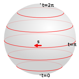
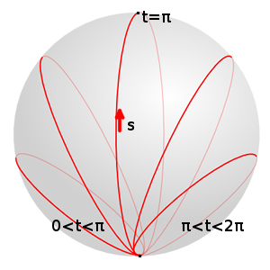
Figure 1. (Left) Images of the $\tilde{B}_{t}$–fields (5.2) and (Right) images of the rotated $\tilde{B}_{t}$–fields (with the $i$–axis pointing upwards and the $j$–axis pointing to the right). The image of the $\tilde{B}_{t}$-field at $t=0$ is the south pole, at $t=\pi$ the equator parametrized clockwise (!) in the $jk$–plane, and at $t=2\pi$ the north pole. All of the rotated $\tilde{B}_{t}$–fields go through the south pole at $s=0$; for small $t$ its images are circles to the left of the south pole, for $t=\pi$ its image is the great circle through the north–pole, and for larger $t$ its images are circles right of the south pole.

Since the spectral flow does not change under rotation (in fact, if $\lambda$ is an eigenspinor of $\mathcal{D}$ satisfying the $(B,\tilde{B}_{t})$ boundary condition, then $\lambda e^{-kt/4}$ is an eigenspinor for the rotated boundary condition, because the rotated $\tilde{B}_{t}$–field is $e^{kt/4}\tilde{B}_{t}e^{-kt/4}$), it is sufficient to compute the spectral flow for $\tilde{B}_{t}$. Because the spectral flow of $\mathcal{D}_{(B,\tilde{B}_{t})}$, $t\in[0,2\pi]$ coincides with the spectral flow of a closed loop of operators, although originally defined as the flow of spectrum through the eigenvalue $\mu=0$, it coincides with the flow of spectrum through any other eigenvalue $\mu\in\mathbb{R}$. We determine the spectral flow by computing the flow through $\mu=-1$.

The crucial information for the computation of the spectral flow of $\mathcal{D}_{(B,\tilde{B}_{t})}$, $t\in[0,2\pi]$ is provided by Lemma 3 which shows that the only parameter compatible with the eigenvalue $\mu=-1$ is $t=\pi$ for which the eigenspace is one dimensional.

To complete the proof of the theorem it therefore remains to compute the sign of the spectral flow. This can be done by the following infinitesimal argument: by “continuity of a finite system of eigenvalues”, cf. [11, IV,3.5], for $t$ in a small neighborhood of $t=\pi$ it is clear that $\mathcal{D}_{(B,\tilde{B}_{t})}$ has a unique eigenvalue close to $-1$ which is necessarily simple.

By Lemma 4, integration of $d\tilde{f}=\bar{\lambda}df\lambda$ for $\lambda$ a simple eigenspinor yields a rotational symmetric immersion $\tilde{f}$. Moreover, by (2.5) the mean curvature $\tilde{H}$ of $\tilde{f}$ is strictly positive for eigenvalues $\mu>-1$ and strictly negative for $\mu<-1$. In the case that $t$ is slightly larger that $\pi$, the $\tilde{B}_{t}$–field is pointing upwards and the immersed disc corresponding to the eigenvalue closest to $\mu=-1$ attains its minimal height (coordinate in $i$–direction) in the interior of the disc. At a point where the minimal height is attained, the tangent plane to the immersion is horizontal and therefore, since the surface normal is downwards, the mean curvature has to be positive. This shows that for $t>\pi$ the eigenvalue closest to $\mu=-1$ is larger than $-1$. The sign of the spectral flow across $\mu=-1$ is thus positive. ∎

Lemma 3.

In the family of Dirac operators $\mathcal{D}_{(B,\tilde{B}_{t})}$, $t\in[0,2\pi]$ with boundary condition (5.2) as in the proof of Theorem 4, only $t=\pi$ has $\mu=-1$ as an eigenvalue. The real dimension of the corresponding eigenspace is one and its non–trivial elements are nowhere vanishing.

Proof.

By (2.5), if $\mathcal{D}_{(B,\tilde{B}_{t})}$ has an eigenspinor $\lambda$ with eigenvalue $\mu=-1$, the immersion obtained by integrating $d\tilde{f}=\bar{\lambda}df\lambda$ is a minimal surface (because $f$ has mean curvature $H=1$).

We first prove that this can only happen in the case that $t=\pi$ for which $\tilde{B}_{t}$ takes values in a plane. To see this, note that the $i$–component $f_{1}$ of the minimal surface $\tilde{f}$ in $\mathbb{R}^{3}=\operatorname{Im}(\mathbb{H})$ is a harmonic function so that by Stokes Theorem

$$\int_{M}df_{1}\wedge*df_{1}=\int_{\partial M}f_{1}*df_{1},$$

where $*$ denotes the complex structure on $T^{*}M$ (i.e., minus the usual Hodge operator). Hence

$$\int_{M}|df_{1}|^{2}dA=\int_{\partial M}f_{1}\tfrac{\partial f_{1}}{\partial\nu}ds$$

with $\frac{\partial}{\partial\nu}$ the (outer) normal derivative of $f_{1}$ along the boundary. Now, up to some positive scale $\tfrac{\partial f_{1}}{\partial\nu}$ equals the $i$–part of $\tilde{B}_{t}$ which is constant and negative for $t<\pi$ while positive for $t>\pi$. Because by choosing a suitable integration constant we can arrange that $f_{1}$ has arbitrary constant sign, we obtain a contradiction unless $t=\pi$ and $f_{1}$ is constant. This shows that $\mu=-1$ can only be eigenvalue of $\mathcal{D}_{(B,\tilde{B}_{t})}$ if $t=\pi$.

A (possibly branched) immersion $\tilde{f}$ obtained from an eigenspinor for $\mu=-1$ is thus planar and hence of the form $j$ times a complex holomorphic function. Up to translation and scaling it coincides with $\tilde{f}(z)=jz$ (because the boundary condition implies that the derivatives of $\tilde{f}$ and $jz$ along the boundary differ only by a real factor which is necessarily constant). In particular, the corresponding spinor is unique up to a real scale and has no zeros.

Conversely, one can check that the eigenspace for $t=\pi$ and $\mu=-1$ is non–empty (and hence real 1–dimensional) by writing down the spinor $\lambda$ which transforms the southern half–sphere $f$ to the standard embedding $\tilde{f}(z)=jz$ of $M$ into $jM$. ∎

Lemma 4.

Let $\mathcal{D}$ be the Dirac operator corresponding to a rotational symmetric immersion $f$ of the disc $M=\{z\in\mathbb{C}\mid|z|\leq 1\}$ and let $(B,\tilde{B})$ be a rotational symmetric boundary condition. If $\mathcal{D}_{(B,\tilde{B})}$ has a real 1–dimensional eigenspace, a corresponding eigenspinor $\lambda$ is rotational symmetric and nowhere vanishing. Integrating $d\tilde{f}=\bar{\lambda}df\lambda$ then yields a rotational symmetric immersion $\tilde{f}$.

Proof.

Assume the rotation $r_{\theta}$ by $\theta\in\mathbb{R}$ of the disc $M$ acts on $\mathbb{R}^{3}=\operatorname{Im}(R)$ by rotation

$$x\in\operatorname{Im}(\mathbb{H})\mapsto e^{-i\theta/2}\,x\,e^{i\theta/2}\in\operatorname{Im}(\mathbb{H})$$

and $f(r_{\theta}(z))=e^{-i\theta/2}f(z)e^{i\theta/2}$ as well as $\tilde{B}(r_{\theta}(z))=e^{-i\theta/2}\tilde{B}(z)e^{i\theta/2}$ for all $z\in M$ and $\theta\in\mathbb{R}$. Then the map

(5.3) $$\lambda\in C^{\infty}(M,\mathbb{H})\mapsto(z\mapsto e^{i\theta/2}\lambda(r_{\theta}(z))e^{-i\theta/2})\in C^{\infty}(M,\mathbb{H})$$

induces a $S^{1}$–representation on the eigenspaces of $\mathcal{D}_{(B,\tilde{B})}$. A spinor $\lambda$ in a real 1–dimensional eigenspace of $\mathcal{D}_{(B,\tilde{B})}$ is thus rotational symmetric, because a real 1–dimensional representation of $S^{1}$ is trivial. Because the zeros of an eigenspinor of $\mathcal{D}_{(B,\tilde{B})}$ are isolated, the rotational symmetric spinor $\lambda$ could only vanish on the axis of rotation. But the asymptotics of eigenspinors at zeros of positive order, see Lemma 3.9 of [8], would not be compatible with the rotational symmetry of $\lambda$. (More generally, a similar argument yields that a spinor that is a higher Fourier mode as in (6.1) has to vanish to order $l$ and therefore gives rise to a branched immersion with a branch point of order $2l$.) ∎

6. Spectral flow and Dirac spectrum of the round 2–sphere $S^{2}$

In the last section of the paper we sketch a relation between the Dirac spectrum of the round 2–sphere and the example of spectral flow discussed in the previous section. In particular, the Dirac spectrum of the round 2–sphere is visualized in Figure 2 and spectral flow is visualized in Figures 4 and 5.

As in the previous section, we denote by $\mathcal{D}_{(B,\tilde{B}_{t})}$ the Dirac operator induced by the immersion $f$ of the unit disc into the southern hemisphere with rotationally symmetric boundary conditions (5.2). The following theorem links its spectrum for $t\in 2\pi\mathbb{Z}$ (when the $\tilde{B}_{t}$–field of the boundary condition is constant and vertical) to the Dirac spectrum of the full round sphere.

Theorem 5.

For $t\in 2\pi\mathbb{Z}$, a branched immersion $\tilde{f}$ with $d\tilde{f}=\bar{\lambda}df\lambda$ for $\lambda$ an eigenspinor of $\mathcal{D}_{(B,\tilde{B}_{t})}$ orthogonally intersects the $jk$–plane along the boundary curve. Reflection in the $jk$–plane extends $\tilde{f}$ to a smooth branched immersion of the sphere. The corresponding extension of the spinor $\lambda$ is an eigenspinor of the Dirac operator for the round 2–sphere.

Proof.

That the boundary curve of $\tilde{f}$ is contained in a plane parallel to the $jk$–plane is clear, because its tangent vector is perpendicular to $\tilde{B}_{t}=\pm i$. Similarly, $\tilde{f}$ intersects this translate of the $jk$–plane orthogonally, because the normal of $\tilde{f}$ is as well perpendicular to $\tilde{B}_{t}$. Reflection of $\tilde{f}$ yields a $C^{2}$–immersion of the sphere. (That the immersion of the full sphere is $C^{1}$ is obvious from the construction. That the second derivative of the full sphere is continuous along the boundary curve of the reflected half–spheres can be proven using that the latter, being contained in the plane of reflection, is a curvature line, so that, with respect to polar coordinates on the parameter domain, the second fundamental form is diagonal along the symmetry axis.) The corresponding extension of the spinor $\lambda$ is thus a $C^{1}$–eigenspinor of the Dirac operator $\mathcal{D}$ for the full round sphere. By elliptic regularity it is smooth and so is the corresponding immersion $\tilde{f}$ of the sphere. ∎

The branched immersions of the sphere thus arising from our Dirac boundary problem for vertical $\tilde{B}_{t}$ are examples of surfaces known as Dirac spheres [15]: a Dirac sphere is an immersion $\tilde{f}$ of the sphere obtained via $d\tilde{f}=\bar{\lambda}df\lambda$ from an eigenspinor $\lambda$ of the Dirac operator $\mathcal{D}$ induced (2.3) by the round immersion $f$ of $S^{2}$ (with $f\colon\mathbb{C}\cup\{\infty\}\rightarrow S^{2}$ denoting the extension of the above parametrization of the southern hemisphere). Dirac spheres are special examples of soliton spheres [17, 3] related to soliton solutions of the mKdV–equation.

Theorem 5 allows to compute the spectrum of $\mathcal{D}_{(B,\tilde{B}_{t})}$ with vertical boundary condition $t\in 2\pi\mathbb{Z}$ from the spectrum of $\mathcal{D}$ for the full unit sphere $S^{2}$. Up to a real shift, $\mathcal{D}$ for $S^{2}$ coincides with the usual spin Dirac operator of the round sphere. Its spectrum is $\{\mu\in\mathbb{Z}\mid\mu\neq-1\}$ with eigenspaces of quaternionic dimension $|\mu+1|$, see e.g. [15] or [16] for references to the physical literature.

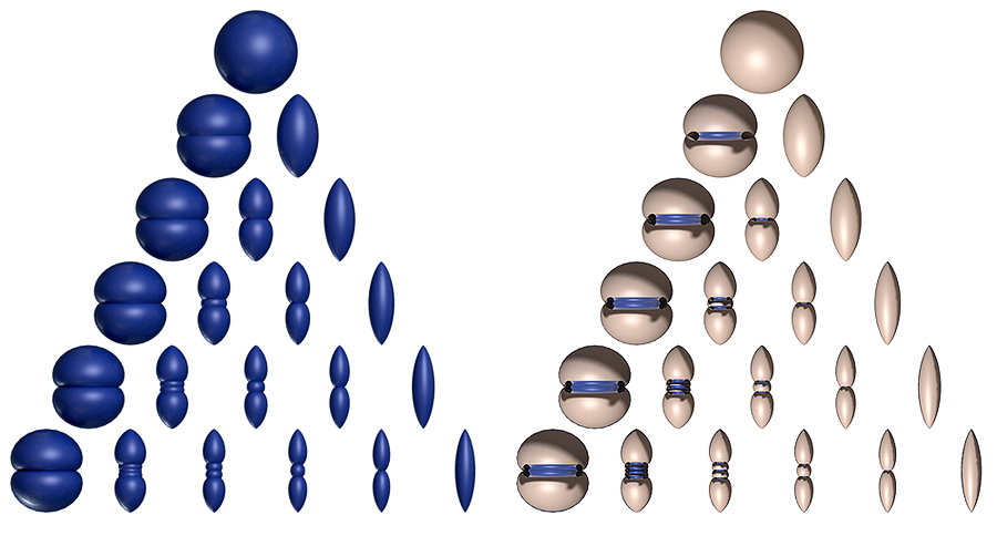
Figure 2. The periodic table of Dirac spheres. Vertical rows show the Dirac spheres corresponding to the canonical basis (6.1) for eigenvalues $\mu=0$, $1$,…, $5$ or, equivalently, $\mu=-2$, $-3$,…,$-7$ (the images for the eigenvalues $\mu$ and $-(2+\mu)$ are the same, as the corresponding branched immersions are geometrically related by point reflections). The leftmost surfaces are immersed surfaces of revolution. The other surfaces rotate with higher frequencies and are branched on the axis of rotation. The frequency raises by two for each step to the right. (Pictures by Keenan Crane)

The spectrum of $\mathcal{D}$ for $S^{2}$ can be visualized by the “periodic table of Dirac spheres”, Figure 2, obtained by Fourier decomposing the quaternionic eigenspace of $\mathcal{D}$ for a given $\mu$ with respect to the $S^{1}$–representation (5.3). This yields a quaternionic basis $\lambda_{l}$, $l=0$,…, $|\mu+1|-1$ satisfying

(6.1) $$\lambda_{l}(r_{\theta}(z))=e^{-i\theta/2}\lambda_{l}(z)e^{i(1/2+l)\theta}.$$

One can check that the branched immersions $\tilde{f}_{l}$, $l=0$,…, $|\mu+1|-1$ obtained from this standard basis via $d\tilde{f}_{l}=\bar{\lambda}_{l}df\lambda_{l}$ are symmetric with respect to the reflection at a translate of the $jk$–plane. Moreover, if $\mu\geq 0$ the restriction of the spinors $\lambda_{l}$ to the unit disc yields a (complex) basis of the $\mu$–eigenspace for the boundary condition $\tilde{B}=i$, while for $\mu\leq-2$ one obtains a basis of the $\mu$–eigenspace for the boundary condition $\tilde{B}=-i$. (Left multiplication by the quaternion $j$ yields a basis for the opposite vertical boundary condition.)

From Section 5 and the preceding discussion we know the eigenspaces of $\mathcal{D}_{(B,\tilde{B}_{t})}$ belonging to the eigenvalues $\mu=-2$, $-1$, and $0$ for $t=0$, $\pi$, and $2\pi$, respectively. The corresponding immersed discs are shown in Figure 3. In contrast to $t=\pi$, for which the $-1$–eigenspace is real 1–dimensional, if $t=0$ or $2\pi$ the $\tilde{B}_{t}$–field is constant and all rotations of the corresponding immersed disc can be obtained from eigenspinors of $\mathcal{D}_{(B,\tilde{B}_{t})}$. This reflects the fact that the eigenspaces for the corresponding eigenvalues $\mu=-2$ and $0$ are then (real) 2–dimensional.

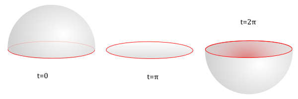
Figure 3. The northern hemisphere, the planar disc, and the original immersion $f$, all with downward orientation, correspond to eigenspinors of $\mathcal{D}_{(B,\tilde{B}_{t})}$ for $t=0$, $\pi$, and $2\pi$ and eigenvalue $-2$, $-1$, and $0$, respectively.

The principle of “continuity of a finite systems of eigenvalues” [11, IV,3.5] suggests that the spectral flow along the path $\mathcal{D}_{(B,\tilde{B}_{t})}$, $t\in[0,2\pi]$ (which is $1$, as shown in the proof of Theorem 4) can be geometrically realized as an “interpolation” between the surfaces shown in Figure 3. Indeed, taking the largest eigenvalue $\mu(t)\leq-1$ of $\mathcal{D}_{(B,\tilde{B}_{t})}$ for every $t\in[0,\pi]$ and the smallest eigenvalue $\mu(t)\geq-1$ of $\mathcal{D}_{(B,\tilde{B}_{t})}$ for every $t\in[\pi,2\pi]$ yields a continuous function $\mu\colon[0,2\pi]\rightarrow\mathbb{R}$. One would expect that, corresponding to $\mu(t)$, $t\in[0,2\pi]$, there is a family of immersed discs similar to Figure 4 which can be obtained from eigenspinors of $\mathcal{D}_{(B,\tilde{B}_{t})}$ for $\mu(t)$. To make this rigorous one has to control whether one can continuously deform eigenspinors through possible bifurcation points $t$ for which $\mu(t)$ is not a simple eigenvalue of $\mathcal{D}_{(B,\tilde{B}_{t})}$. As indicated in Figure 4, it should be possible to realize spectral flow by a deformation through surfaces of revolution. This can be checked by spectral theory for 1–dimensional Dirac operators.

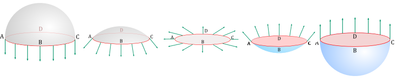
Figure 4. Expected qualitative behavior of immersions corresponding to eigenspinors realizing the spectral flow occurring in the proof of Theorem 4 (as $t$ goes from $0$ to $2\pi$ and $\mu$ from $-2$ to $0$).

A similar analysis should show that the spectral flow of $\mathcal{D}_{(B,\tilde{B}_{t})}$ for $t$ between $2\pi k$ and $2\pi(k+1)$, $k\in\mathbb{Z}$, and $\mu$ between $l\in\mathbb{Z}\backslash\{-1,-2\}$ and $l+1$ can be geometrically realized by a deformation through surfaces of revolution obtained from eigenspinors of $\mathcal{D}_{(B,\tilde{B}_{t})}$. See e.g. Figure 5 for the expected deformation between $\mu=-2$ and $\mu=-3$.

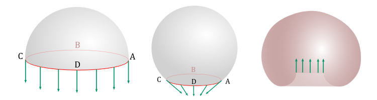
Figure 5. Expected qualitative behavior of immersions corresponding to eigenspinors realizing the spectral flow for the boundary condition (5.2) as $t$ goes from $0$ to $-2\pi$ and $\mu$ from $-2$ to $-3$.

Summary: We conclude the paper by summarizing the preceding discussion of the family $\mathcal{D}_{(B,\tilde{B}_{t})}$ of Dirac operators induced by the round half–sphere with periodic bi–normal boundary conditions. The arising picture is the following:

• for vertical boundary conditions $t\in 2\pi\mathbb{Z}$ the spectrum of $\mathcal{D}_{(B,\tilde{B}_{t})}$ coincides with the spectrum of the full round sphere (Theorem 5) and

• the spectral flow under a half rotation $t\leadsto t+2\pi$ of the bi–normal field is one (Theorem 4).

This means that, upon a half rotation of the bi–normal field from $t=2\pi k$ to $2\pi(k+1)$, $k\in\mathbb{Z}$, all eigenvalues flow upwards with multiplicity one (otherwise said, after a half rotation the spectrum itself is unchanged, but when viewing the eigenvalues taken with their multiplicities as an ordered sequence of real numbers that continuously depend on $t$, under $t\leadsto t+2\pi$ all eigenvalues move up one step in this ordered sequence of eigenvalues).

One would expect that one can follow this upward flow of eigenvalues by a continuous family of eigenspinors for the respective eigenvalues. This would allow to realize spectral flow geometrically by immersed discs, presumably with rotational symmetry. Assuming this is possible,

• the upward flow of eigenvalues in the negative part of the spectrum $\mu<-2$ would amount to “continuously” climbing up on the leftmost side in the periodic table of Dirac spheres in Figure 2 (for the expected “backward” flow $t\leadsto t-2\pi$ from $-2$ to $-3$, see Figure 5),

• the flow from $\mu=-2$ to $\mu=0$ would “continuously” interpolate between half–spheres with opposite orientations (see Figure 4), and

• the upward flow in the positive part $\mu\geq 0$ would amount to going down “continuously” on the leftmost side in the periodic table of Dirac spheres in Figure 2.

This indicates that geometrically the spectral flow in our example corresponds to “wrapping up” the disc/half–sphere by rotating its bi–normal field around the boundary curve. From this perspective spectral flow appears as a continuous geometric realization of the process of “adding solitons”.

References

- [1] Atiyah, M.F., Patodi, V.K., and Singer, I.M., Spectral asymmetry and Riemannian geometry. III Math. Proc. Camb. Phil. Soc. (1976) 79, 71–99.
- [2] Bär, C. and Ballmann, W., Boundary value problems for elliptic differential operators of first order. ArXiv:1101.1196v1, to appear in Surveys in Differential Geometry (2012) XVII, 1–78.
- [3] Bohle, C. and Peters, G.P., Soliton spheres, Trans. Amer. Math. Soc. 363 (2011), 5419–5463.
- [4] Booss, B. and Bleecker, D.D., Topology and Analysis. The Atiyah–Singer Index Formula and Gauge–Theoretic Physics. Springer, Berlin, 1985.
- [5] Booss-Bavnbek, B., Lesch, M., and Phillips, J., Unbounded Fredholm operators and spectral flow. Canad. J. Math. 57 (2005), 225–250.
- [6] Burstall, F. E., Ferus, D., Leschke, K., Pedit, F., and Pinkall, U., Conformal geometry of surfaces in and quaternions. Lecture Notes in Mathematics 1772, Springer, Berlin, 2002.
- [7] Crane, K., Pinkall, U., and Schröder, P., Spin transformations of discrete surfaces. ACM Transactions on Graphics, Proceedings of ACM SIGGRAPH 2011, 30 (2011), Article No. 104.
- [8] Ferus, D., Leschke, K., Pedit, F., and Pinkall. U., Quaternionic holomorphic geometry: Plücker formula, Dirac eigenvalue estimates and energy estimates of harmonic 2–tori. Invent. Math. 146 (2001), 507–593.
- [9] Hörmander, L., Linear partial differential operators. Springer, Berlin, 1963.
- [10] Kamberov, G., Pedit, F., and Pinkall, U., Bonnet pairs and isothermic surfaces. Duke Math. J. 92 (1998), 637–644.
- [11] Kato, T., Perturbation theory for linear operators. Springer, Berlin, 1966/1976.
- [12] Pedit, F. and Pinkall U., Quaternionic analysis on Riemann surfaces and differential geometry. Doc. Math. J. DMV, Extra Volume ICM Berlin 1998, Vol. II, 389–400.
- [13] Phillips, J., Self-adjoint Fredholm operators and spectral flow. Canad. Math. Bull. 39 (1996), 460–467.
- [14] Pinkall, U., Regular homotopy classes of immersed surfaces. Topology 24 (1985) 421–434.
- [15] Richter, J., Conformal maps of a Riemann surface into the space of quaternions. Thesis, TU–Berlin, 1997.
- [16] Szmytkowski, R., Recurrence and differential relations for spherical spinors J. Math. Chem. 42 (2007) 397–413.
- [17] Taimanov, I.A., The Weierstrass representation of spheres in , the Willmore numbers, and soliton spheres. Proc. Steklov Inst. Math. 225 (1999), 322–343.
- [18] Taimanov, I.A., The two–dimensional Dirac operator and the theory of surfaces. Russian Math. Surveys 61 (2006), 79–159.