Response of the Jovian thermosphere to a transient ‘pulse’ in solar wind pressure

Abstract

The importance of the Jovian thermosphere with regard to magnetosphere-ionosphere coupling is often neglected in magnetospheric physics. We present the first study to investigate the response of the Jovian thermosphere to transient variations in solar wind dynamic pressure, using an azimuthally symmetric global circulation model coupled to a simple magnetosphere and fixed auroral conductivity model. In our simulations, the Jovian magnetosphere encounters a solar wind shock or rarefaction region and is subsequently compressed or expanded. We present the ensuing response of the coupling currents, thermospheric flows, heating and cooling terms, and the aurora to these transient events. Transient compressions cause the reversal, with respect to steady state, of magnetosphere-ionosphere coupling currents and momentum transfer between the thermosphere and magnetosphere. They also cause at least a factor of two increase in the Joule heating rate. Ion drag significantly changes the kinetic energy of the thermospheric neutrals depending on whether the magnetosphere is compressed or expanded. Local temperature variations appear between ${\sim}{-}45\mbox{ and }175\,\mathrm{K}$ for the compression scenario and ${\sim}{-}20\mbox{ and }50\,\mathrm{K}$ for the expansion case. Extended regions of equatorward flow develop in the wake of compression events - we discuss the implications of this behaviour for global energy transport. Both compressions and expansions lead to a ${\sim}2000\,\mathrm{TW}$ increase in the total power dissipated or deposited in the thermosphere. In terms of auroral processes, transient compressions increase main oval UV emission by a factor of ${\sim}4.5\,\mathrm{}$ whilst transient expansions increase this main emission by a more modest $37\,\mathrm{\%}$. Both types of transient event cause shifts in the position of the main oval, of up to $1\,\mathrm{{}^{\circ}}$ latitude.

1 Introduction

1.1 Jovian magnetosphere-ionosphere coupling

The interaction between the Jovian magnetosphere and ionosphere is complex. The current systems which connect the planet’s ionosphere and magnetosphere are controlled by a feedback mechanism involving the rotation of magnetospheric plasma, the conductance of the ionosphere and the wind system prevailing in the thermosphere (upper atmosphere). Several studies, however, have made substantial progress in modelling this interaction (Hill, 1979; Pontius, 1997; Hill, 2001; Cowley and Bunce, 2001, 2003a, 2003b; Nichols and Cowley, 2004; Cowley et al., 2005; Bougher et al., 2005; Cowley et al., 2007; Majeed et al., 2009; Tao et al., 2009; Ray et al., 2010; Nichols, 2011; Ray et al., 2012). The models of Cowley and Bunce (2003a, b); Nichols and Cowley (2004) were primarily used to study the interaction of the inner and middle magnetosphere and how these regions couple with the Jovian ionosphere; Cowley et al. (2005) and Cowley et al. (2007) expanded on the former studies by incorporating simplified models for the outer magnetosphere and polar cap region, and thus coupling the ‘entire’ magnetosphere to the ionosphere. Nichols (2011) considered how a whole magnetosphere self-consistently interacted with the magnetosphere-ionosphere system. The force balance formalism of Caudal (1986) was used in the Nichols (2011).

In addition, Cowley and Bunce (2003a, b) and Cowley et al. (2007) investigated how the coupled magnetosphere-ionosphere (M-I) system interacts with the solar wind - specifically, transient variations in the solar wind dynamic pressure which cause compressions and expansions of the magnetosphere. These models have made realistic predictions regarding the corresponding response of magnetospheric and ionospheric currents, plasma angular velocity profiles and auroral emission (both in terms of the intensity of emission and its location in the ionosphere). Many of these model predictions are supported by observations and complementary theoretical studies such as Nichols et al. (2009); Clarke et al. (2009) and Southwood and Kivelson (2001). None of these aforementioned studies, however, have self-consistently accounted for the dynamics of the Jovian thermosphere. In these studies the thermosphere is assumed to have an angular velocity ${\Omega_{T}}$, independent of altitude, which is derived from a constant ‘slippage factor’, ${K}$, given by

$${K} ={\frac{\left(\Omega_{J}-\Omega_{T}\right)}{\left(\Omega_{J}-\Omega_{M}\right)}}.$$ (1)

In this expression ${\Omega_{J}}$ ($1.76{\times}10^{-4}\,\mathrm{rad\,s^{-1}}$) is the angular velocity of the planet and ${\Omega_{M}}$ is the angular velocity of the magnetospheric region conjugate to the thermosphere. This ensures the ordering ${\Omega_{J}>\Omega_{T}>\Omega_{M}}$, for a steady state, where angular momentum is transferred from ionosphere to magnetosphere.

Smith and Aylward (2009) expanded further on the current body of M-I models by coupling a simplified magnetosphere model with an azimuthally symmetric Global Circulation Model (GCM) of Jupiter. Their approach allowed for the self-consistent calculation of the Jovian thermospheric angular velocity, in a coupled M-I system which had reached a steady state.

The study by Smith and Aylward (2009) produced some notable results such as:

i) Angular momentum transfer: meridional advection of momentum, rather than vertical viscous transport, is the main mechanism for transferring angular momentum in the high latitude thermosphere.

ii) Thermospheric super-corotation: largely due to (i), the thermosphere super-corotates (${\Omega_{T}}{=}1.05\,\mathrm{\Omega_{J}}$) throughout those latitudes (${\sim}65{-}73\,\mathrm{{}^{\circ}}$) where it magnetically maps to the middle magnetosphere (${\sim}6{-}25\,\mathrm{R_{J}}$).

iii) Distribution of heat: the simulated thermospheric winds develop two main cells of meridional flow, which cool lower latitudes (${\lesssim}75\,\mathrm{{}^{\circ}}$) whilst heating the polar regions (${\gtrsim}80\,\mathrm{{}^{\circ}}$).

Yates et al. (2012) used the model of Smith and Aylward (2009) to study the influence of the solar wind on steady-state thermospheric flows of Jupiter. They found that ionospheric and magnetospheric currents, thermospheric powers, temperature and auroral emission (by proxy of field-aligned current (FAC)) all exhibit increases with decreasing solar wind dynamic pressure (from $0.213\,\mathrm{nPa}$ to $0.021\,\mathrm{nPa}$ (Joy et al., 2002)).

Southwood and Kivelson (2001) suggested that a magnetospheric compression would cause an increase in the degree of magnetospheric plasma corotation (i.e. the quantity $(\Omega_{J}-\Omega_{M})$ would decrease), and this would consequently lead to a sizeable decrease in M-I coupling currents and auroral emission. They also argued that the reverse would be true for a magnetospheric expansion. Simulations by Cowley et al. (2007) and Yates et al. (2012) confirmed these predictions, provided that the system is given enough time to achieve steady-state (${\geq}50\,\mathrm{}$ rotations). On the other hand, the studies of Cowley and Bunce (2003a, b) and more recently, of Cowley et al. (2007) simulated the ‘transient’ (short-term) response of the system to rapid (${\sim}2-3\,\mathrm{hours}$) magnetospheric compressions and expansions. This short-term behaviour was found to differ from the steady state case. For rapid compressions (${\lesssim}3\,\mathrm{hours}$), the conservation of plasma angular momentum causes the magnetosphere to super-corotate compared to the planet and thermosphere. The flow shear between the thermosphere and magnetosphere, represented by $(\Omega_{T}-\Omega_{M})$, is now negative and leads to current reversals at magnetic co-latitudes that are conjugate to the middle and outer magnetospheres (${\sim}10{-}17\,\mathrm{{}^{\circ}}$). Negative flow shear also causes energy to be transferred from the magnetosphere to thermosphere; in contrast to the steady-state, where energy is transferred from the thermosphere to the magnetosphere, in order to accelerate outflowing, magnetospheric plasma towards corotation. For transient expansions, Cowley et al. (2007) showed that ${\Omega_{M}}$ decreases but the flow shear increases, leading to a ${\sim}500\,\mathrm{\%}$ increase in the intensity of M-I currents (for an expansion from a dayside magnetopause radius of $45\,\mathrm{R_{J}}$ to $85\,\mathrm{R_{J}}$, ${R_{J}}{=}71492\,\mathrm{km}$).

For these transient events, where the magnetopause is displaced by ${\sim}40\,\mathrm{R_{J}}$, Cowley et al. (2007) predict differing auroral responses dependent on the nature of the event (compression or expansion). For compressions, electron energy flux (${\sim}10\,\mathrm{\%}$ of which is used to produce ultraviolet (UV) aurora) at the open-closed field line boundary (polar emission) increases by two orders of magnitude, whilst the main emission is halved. In the expansion case, there is a 30-fold increase in main emission mapping to the middle magnetosphere, whilst polar emission decreases to ${\sim}2\,\mathrm{\%}$ of its steady-state value. Recent observations of auroral emission by Clarke et al. (2009) show a factor of two increase in total ultraviolet (UV) auroral power, near the arrival of a solar wind compression region, typically corresponding to an increase in solar wind dynamic pressure of ${\sim}0.01{-}0.3\,\mathrm{nPa}$. Furthermore, Nichols et al. (2009) showed, using the same Hubble Space Telescope (HST) images as Clarke et al. (2009), that this increase in auroral emission consists of approximately even contributions from the so-called ‘main oval’ and the high-latitude polar emission. Nichols et al. (2009) also showed that the location of the ‘main oval’ shifted polewards by ${\sim}1\,\mathrm{{}^{\circ}}$ in response to solar wind pressure increase of an order of magnitude. For a rarefaction region in the solar wind, an order of magnitude decrease in solar wind pressure, Clarke et al. (2009) observed little, if any, change in auroral emission.

1.2 Jovian atmospheric heating

The Jovian upper atmospheric temperature is up to $700\,\mathrm{K}$ higher than that predicted by solar heating alone (Strobel and Smith, 1973; Yelle and Miller, 2004). This ‘energy crisis’ at Jupiter and the other giant planets has puzzled scientists for over $40\,\mathrm{}$ years. Different theories have been put forward to explain Jovian upper atmospheric heating: gravity waves (Young et al., 1997), auroral particle precipitation (Waite et al., 1983; Grodent et al., 2001), Joule heating (Waite et al., 1983; Eviatar and Barbosa, 1984) and ion drag (Miller et al., 2000; Smith et al., 2005; Millward et al., 2005). None of the aforementioned studies have been able to fully account for the observations.

M-I coupling models by Achilleos et al. (1998); Bougher et al. (2005); Smith and Aylward (2009); Tao et al. (2009); Yates et al. (2012) have all discussed steady-state heating and cooling terms in the Jovian thermosphere. Yates et al. (2012), whilst investigating the influence of solar wind on the steady-state thermospheric flows of Jupiter, found that ion drag energy and Joule heating increased by ${\lesssim}200\,\mathrm{\%}$ (from a compressed to expanded magnetospheric configuration) resulting in a thermospheric temperature increase of ${\sim}135\,\mathrm{K}$. Cowley et al. (2007) discussed ‘transient’ heating and dynamics in terms of power dissipated in the thermosphere via Joule heating and ion drag energy, as well as power used to accelerate magnetospheric plasma. Cowley et al. (2007) considered displacements of the Jovian magnetopause by ${\sim}40\,\mathrm{R_{J}}$. They found that, for compressions, there was a net transfer of power from magnetosphere to planet of ${\sim}325\,\mathrm{TW}$, due to the expected super-corotation of magnetospheric plasma. For expansions, Cowley et al. (2007) found that the power dissipated in the thermosphere (and used to accelerate magnetospheric plasma) increased by a factor of ${\sim}2.5\,\mathrm{}$ resulting from a large increase in azimuthal flow shear between the expanded magnetosphere and the thermosphere.

Melin et al. (2006) analysed infrared data from an auroral heating event observed by Stallard et al. (2001, 2002) (from September 8-11, 1998) and found that particle precipitation could not account for the observed increase in ionospheric temperature ($940{-}1065\,\mathrm{K}$). The combined estimate of ion drag and Joule heating rates increased from $67\,\mathrm{mW\,m^{-2}}$ (on September 8) to $277\,\mathrm{mW\,m^{-2}}$ (on September 11) resulting from a doubling of the ionospheric electric field (inferred from spectroscopic observations); this increase in heating was able to account for the observed rise in temperature. Cooling rates (by Hydrocarbons and ${H_{3}^{+}}$ emission) also increased during the event but only by ${\sim}20\,\mathrm{\%}$ of the total inferred heating rate. Thus, a net increase in ionospheric temperature resulted. More detailed analysis showed that these cooling mechanisms would be unlikely to return the thermosphere to its initial temperature before the onset of subsequent heating events. Melin et al. (2006) thus concluded that the temperature increases could plausibly lead to an increase in equatorward winds, which transport thermal energy to lower latitudes (Waite et al., 1983).

In this study, we use the Yates et al. (2012) model, ‘JASMIN’ (Jovian Axisymmetric Simulator, with Magnetosphere, Ionosphere and Neutrals), to estimate the response of Jovian thermospheric dynamics, heating and aurora to transient changes in the solar wind dynamic pressure and, consequently, magnetospheric size. By transient, we mean changes on time scales ${\lesssim}3\,\mathrm{hours}$, where the angular momentum of the magnetospheric plasma is approximately conserved (Cowley et al., 2007) as the time scales required for changes in the M-I currents to affect ${\Omega_{M}}$ are much longer, ${\sim}10{-}20\,\mathrm{hours}$. Our coupled model responds to time-dependent profiles of plasma angular velocity in the magnetosphere. We employ different ${\Omega_{M}(\rho_{e},t)}$ profiles (${\rho_{e}}$ represents equatorial radial distance; ${t}$ denotes time) to represent compressions and expansions of the middle magnetosphere. This is the first study to investigate how time-dependent variations in solar wind pressure influence both magnetospheric and thermospheric properties of the Jovian system, and to use a realistic GCM to represent the thermosphere.

In section 2 we summarise the time scales involved in the Jovian system and section 3 describes the model used in this study. In sections 4 and 5 we present our findings for the transient compression and expansion scenarios respectively. We discuss our findings and and their limitations in section 6 and conclude in section 7.

2 Time-dependence of the Jovian system

Variations in magnetic field, plasma angular velocity and thermospheric flow patterns due to solar wind pressure changes present challenges for modelling the Jovian system. Various time-scales, such as those associated with M-I coupling, compression or expansion of the magnetosphere and thermospheric response, need to be considered. The studies by Cowley and Bunce (2003a, b) and Cowley et al. (2007) are among the few to have addressed these issues, using the simplifying approximations discussed hereafter.

i) M-I coupling time scale: The neutral atmosphere transfers angular momentum to the magnetosphere along magnetic field lines in order to accelerate the radially outflowing magnetospheric plasma towards corotation. The time-scale on which this angular momentum is transferred has been estimated by Cowley and Bunce (2003a) to be ${\sim}5{-}20\,\mathrm{}$ hours, similarly to that found by Vasyliunas (1994).

ii) Compression (and expansion) of the magnetosphere: Large changes in magnetospheric size (${\sim}40\,\mathrm{R_{J}}$) can occur when the Jovian magnetosphere encounters a sudden change in solar wind dynamic pressure, such as would be caused by a Coronal Mass Ejection (CME) or Corotating Interaction Regions (CIR). Cowley and Bunce (2003a) and Cowley et al. (2007) considered compressions (and expansions) occurring over ${\sim}2{-}3\,\mathrm{hours}$, and were thus able to assume conservation of plasma angular momentum when calculating the response of the M-I system, since the coupling time scale discussed in i) is large, by comparison.

iii) Thermospheric response time: The thermosphere and magnetosphere are coupled together via ion-neutral collisions in the ionosphere; therefore a change in plasma angular velocity would cause a corresponding change in the thermosphere’s effective angular velocity. Recent models for the thermospheric response are generally divided in two scenarios: (i) A system where the thermosphere responds promptly, on the order of a few tens of minutes as found by (Millward et al., 2005), and (ii) a system where the thermosphere responds on the order of two days and, as such, is essentially unresponsive to transient events (Gong, 2005). However, in this study, we do not make a distinction between thermospheric response models. We simply allow the GCM to respond self-consistently to the imposed changes in plasma angular velocity assumed for the transient compressions and expansions, thus allowing a realistic, thermospheric response to these changes.

3 Model description

3.1 Thermosphere model

The thermosphere model used in this study is a GCM which solves the non-linear Navier-Stokes equations of energy, momentum and continuity, using explicit time integration (Müller-Wodarg et al., 2006). The Müller-Wodarg et al. (2006) three-dimensional (3-D) GCM was created for Saturn’s thermosphere, and later modified for Saturn and Jupiter respectively in Smith and Aylward (2008) and Smith and Aylward (2009). It is the Smith and Aylward (2009) modified GCM that we use in this study. The model assumes azimuthal symmetry, and is thus two-dimensional (pressure/altitude and latitude) whilst still solving the 3-D equations. The Navier-Stokes equations are solved in the pressure coordinate system, providing time dependent distributions of thermospheric wind, temperature and energy. The zonal and meridional momentum equations, and the energy equation forming the basis of this particular GCM can be found in Achilleos et al. (1998); Müller-Wodarg et al. (2006) or Tao et al. (2009), should the reader be interested. Our model is resolved on a $0.2\,\mathrm{{}^{\circ}}$ latitude and $0.4\,\mathrm{}$ pressure scale height grid, with a lower boundary at $2\,\mathrm{\mu bar}$ ($300\,\mathrm{km}$ above the $1\,\mathrm{bar(B)}$ level) and upper boundary at $0.02\,\mathrm{nbar}$.

3.2 Ionosphere model

We employ a simplified model of the ionosphere used in Smith and Aylward (2009) and Yates et al. (2012), who separate the model into two components: i) a vertical part describing the relative change of conductivity with altitude, as defined by the 1D model of Grodent et al. (2001). ii) A horizontal part, which linearly scales the Grodent et al. (2001) model at all altitudes so that the height-integrated Pedersen conductance ${\Sigma_{P}}$ matches a global pattern prescribed by the user. The sole difference between the model used in Yates et al. (2012) and that presented here lies in the horizontal part. Here we employ a fixed value of ${\Sigma_{P}}$ between latitudes $60\,\mathrm{{}^{\circ}}$ and $74\,\mathrm{{}^{\circ}}$ whilst in the above studies, conductances in this region may be enhanced, above background levels, by FACs (Nichols and Cowley, 2004). Table 1 shows the three different height-integrated Pedersen conductance regions employed in our model, their corresponding ionospheric latitudes and their assigned values of ${\Sigma_{P}}$. Section 6.4 discusses the limitations in using such assumptions.

3.3 Magnetosphere model

The axisymmetric Jovian magnetosphere model employed in this study is the same as that described in Yates et al. (2012). It combines a detailed model of the inner and middle magnetosphere (Nichols and Cowley, 2004) with a simplified model of the outer magnetosphere and region of open field lines (Cowley et al., 2005). The ability to reconfigure the magnetosphere depending on its size is also included by assuming that magnetic flux is conserved (Cowley et al., 2007). Surfaces of constant flux function define shells of magnetic field lines with common equatorial radii ${\rho_{e}}$ and ionospheric co-latitude ${\theta_{i}}$. These surfaces also allow for the magnetic mapping from the equatorial plane of the magnetodisc (middle magnetosphere) to the ionosphere. This mapping requires an ionospheric flux function ${F_{i}(\theta_{i})}$, a magnetospheric counterpart ${F_{e}(\rho_{e})}$ (representing the magnetic flux integrated between a given equatorial radial distance ${\rho_{e}}$ and infinity) and the equality ${F_{i}(\theta_{i})}{=}{F_{e}(\rho_{e})}$, which represents the mapping between ${\theta_{i}}$ and ${\rho_{e}}$ to which the corresponding magnetic field line extends (Nichols and Cowley, 2004). The ionospheric flux function is given by:

$${F_{i}}={B_{J}\rho_{i}^{2}}={B_{J}R_{i}^{2}\sin^{2}\theta_{i}},$$ (2)

where ${B_{J}}$ is the equatorial magnetic field strength at the planet’s surface and ${\rho_{i}}$ is the perpendicular distance to the planet’s magnetic/rotation axis (${\rho_{i}}{=}{R_{i}\sin\theta_{i}}$, where ${R_{i}}$ is the ionospheric radius. We adopt ${B_{J}}{=}426400\,\mathrm{nT}$ (Connerney et al., 1998), and ${R_{i}}{=}67350\,\mathrm{km}$ (Cowley et al., 2007). Note ${R_{i}}{<}{R_{J}}$ due to polar flattening at Jupiter. For further details on the magnetosphere model employed here the reader is referred to Yates et al. (2012) and the references therein. A discussion on the currents which couple our model can be found in A.

3.4 Obtaining the transient plasma angular velocity

In steady state, plasma angular velocity profiles are obtained in a similar manner to that discussed in Smith and Aylward (2009) and Yates et al. (2012); by solving the Hill-Pontius equation in the inner and middle magnetosphere, but assuming a constant Pedersen conductance.

We now discuss the calculation of plasma angular velocity once the model has entered the transient regime i.e. once our initial, steady-state system begins to undergo a transient compression/expansion of the magnetosphere. Our method of calculating transient plasma angular velocities follows that of Cowley et al. (2007). Prior to the rapid compression or expansion, the system exists in a steady state, with plasma angular velocity ${\Omega_{M}(\theta_{i},t{=}0)}$ as a function of co-latitude ${\theta_{i}}$ and time ${t}$. Using the magnetic mapping method discussed in section 3.3, the equatorial radial distance ${\rho_{e}(\theta_{i},t{=}0)}$ of the local field line can be found. The arrival of the solar wind pulse or rarefaction causes the magnetosphere to compress or expand by several tens of ${R_{J}}$ (typical choice for the simulations) and the model enters the transient (time-dependent) regime. Thus, a given co-latitude ${\theta_{i}}$ now maps to a new radial distance ${\rho_{e}(\theta_{i},t)}$. If, as discussed in section 2, the solar wind pulse causes perturbations that occur on sufficiently small time scales (${\sim}2{-}3\,\mathrm{hours}$), we can assume that plasma angular momentum is approximately conserved. The plasma angular velocity profile throughout the ‘pulse’ in solar wind pressure is then given by:

$${\Omega_{M}(\theta_{i},t)}= {\Omega_{M}(\theta_{i},t{=}0)\left(\frac{\rho_{e}(\theta_{i},t{=}0)}{\rho_{e}(\theta_{i},t)}\right)^{2}},$$ (3)

where the notation ${t{=}0}$ and ${t}$ denote the initial (steady-state) and transient state (at each time-step throughout the event) respectively.

For this study, the time evolution of solar wind dynamic pressure, and thus magnetodisc size, is represented by a Gaussian function. ${R_{MM}(t)}$ represents the magnetodisc radius as a function of time and is given by

$${R_{MM}(t)}={Ae^{-\frac{\left(t-t_{o}\right)^{2}}{2\Delta t^{2}}}}+{R_{MMO}},$$ (4)

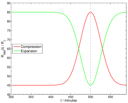
Figure 1: The variation of magnetodisc radius ${R_{MM}(t)}$ with time during a pulse in the solar wind. The red and green lines represent a compression and expansion respectively throughout the entire pulse. The grey dashed line indicates the point of maximum variation.

where ${A}{=}{R_{MM}(t_{o})-R_{MMO}}$ and is the amplitude of the corresponding curve, ${R_{MMO}}$ is the initial magnetodisc radius, ${R_{MM}(t_{o})}$ is the maximum or minimum radius, ${t_{o}}$ is the time at which ${R_{MM}(t)}{=}{R_{MM}(t_{o})}$ ($90\,\mathrm{minutes}$ after pulse start time ${t_{s}}$), and ${\Delta t}$ controls the width of the ‘bell’ (obtained using ${(2/3)(t_{o}-t_{s})}={2\sqrt{2\ln 2}\,\,\Delta t}$ ). After achieving steady-state, we run the model for a single Jovian day, transient mode is then initialised $3\,\mathrm{hours}$ prior to the end of the Jovian day (and model runtime). Profiles of ${R_{MM}(t)}$ for compressions and expansions are shown in Fig. 1.

As indicated in Fig. 1, the simulated pulse lasts for a total of three hours, after which the magnetodisc returns to its initial size. This is represented by the red (compression) and green (expansion) lines. The black dashed line indicates the point of maximum compression/expansion (at $t{=}{t_{o}}$) where we take a ‘snapshot’ of model outputs in order to investigate the thermospheric response midway through the transient pulse (henceforth, this phase of the event is referred to as ‘half-pulse’).

As in Yates et al. (2012), we divided the magnetosphere into four regions: region I, representing open field lines of the polar cap; region II containing the closed field lines of the outer magnetosphere; region III (shaded in figures) is the middle magnetosphere (magnetodisc) where we assume the Hill-Pontius equation is valid for steady-state conditions. Region IV is the inner magnetosphere (which is assumed to be fully corotating in steady state). Region III is our main region of interest throughout this study since it plays a central role in determining the morphology of auroral currents.

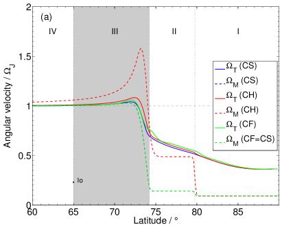
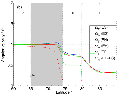
Figure 2: (a) Thermospheric and plasma angular velocity profiles for the transient compression cases as a function of ionospheric latitude. Solid lines represent thermospheric profiles whilst dashed lines represent plasma profiles. The blue lines represent case CS (steady state before compression) whilst the red and green lines indicate cases CH (system at minimum disc radius) and CF (system just returned to initial disc radius) respectively. The magnetospheric regions (region III shaded) are labelled and separated by the black dotted lines. The magnetically mapped location of Io on the ionosphere is marked and labelled. (b) Thermosphere and plasma angular velocity profiles for the transient expansion cases as a function of ionospheric latitude. The line styles are the same as (a) but the cases are now ES, EH and EF respectively, where ‘E’ denotes expansion, and the ‘S’, ‘H’ and ‘F’ symbols represent the same phases of the event as for Fig. 2a.

Plasma velocities are shown in Fig. 2a-b (dashed lines) along with their corresponding thermospheric angular velocities (solid lines). Fig. 2a shows angular velocity profiles pertaining to the transient compression scenario. The starting configuration (steady-state) is indicated by blue lines and is henceforth, referred to as ‘case CS’ (pre-Compression Steady-state). Halfway through the pulse, when the magnetodisc radius is a minimum, angular velocity profiles are represented by red lines and will be referred to as case CH (Compression Half-pulse). Case CF (Compression Full-pulse) profiles are indicated by green lines and represent the state of the system after the pulse subsides (see Table 2 for description of different cases). In Fig. 2a, there is significant super-corotation of the magnetodisc plasma throughout most of regions IV and III. Plasma rotating faster than both the thermosphere and deep planet creates a reversal of currents and angular momentum transfer between the ionosphere and magnetosphere (Cowley et al., 2007). Thus angular momentum is transported from the magnetosphere to the thermosphere, where rotation rate increases from its initial state. We see an average of ${\sim}3\,\mathrm{\%}$ increase in peak ${\Omega_{T}}$ in response to the transient compression event. This is small compared to the factor of two increase in peak ${\Omega_{M}}$ (for case CH). The significant difference in response between the thermosphere and magnetosphere is due to the larger mass of the neutral thermosphere and thus, its greater resistance to change (inertia). After the subsidence of the pulse, the magnetosphere returns to its initial size and, thus, the ${\Omega_{M}}$ profile for case CF is equal to that of CS at all latitudes. The same cannot be said for the thermospheric angular velocities; the CF thermosphere rotates slightly faster (${\sim}2\,\mathrm{\%}$ at maximum ${\Omega_{T}}$) for parts of regions III and I and all of region II. This comparison highlights the difference in response between the thermosphere and magnetosphere to the prescribed changes in solar wind pressure.

Fig. 2b shows angular velocity profiles corresponding to the transient expansion scenario. Like the compression scenario, we have cases ES (pre-Expansion Steady-state (initial value of ${R_{MM}{=}45\,{R_{J}}}$)), EH (Expansion Half-pulse ${R_{MM}{=}85\,{R_{J}}}$) and EF (Expansion Full-pulse) indicated by blue, red and green lines respectively. The behaviour is very different from the compression: midway through the event (case EH), the magnetodisc plasma sub-corotates to an even greater degree in regions IV and III compared to the initial steady-state case, ES. The thermosphere also sub-corotates to a greater degree, but maintains a higher angular velocity than the disc plasma, meaning that current reversal does not occur. Thermospheric angular velocities for cases ES and EF differ slightly, as in the compression scenario i.e due to the greater lag in the thermospheric response time.

Fig. 2 theoretically demonstrates the effect that transient shocks and rarefactions in the solar wind have on both plasma and thermospheric angular velocities. Sections 4 and 5 will discuss the effects on the M-I coupling currents and the global thermospheric dynamics.

4 Magnetospheric Compressions

In this section we present findings for our transient magnetospheric compression scenario which lasts for a total of three hours.

4.1 Auroral currents

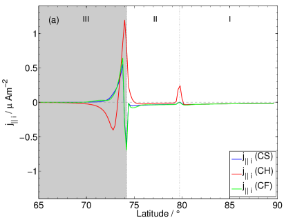
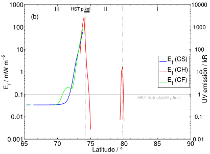
Figure 3: (a) FAC densities in the high latitude ionospheric region for our transient compression cases. The blue line represents case CS whilst the red and green lines indicate cases CH and CF respectively. The conjugate magnetospheric regions (region III is shaded) are separated by dotted black lines and labelled. (b) Shows the latitudinal variation of the precipitating electron flux (on the left axis) and the corresponding UV auroral emission (on the right axis) for the transient compression cases. The colour codes and in plot labels are the same as (a). The latitudinal size of an ACS-SBC HST pixel located near the main auroral emission is represented by the dark grey box. The solid grey line indicates the limit of detectability of the HST (Cowley et al., 2007).

Fig. 3a shows FAC density as a function of latitude (computed from the horizontal divergence of ${I_{P}}$ (ionospheric Pedersen current density); see Eq. (7)) for cases CS, CH and CF. The blue line represents case CS, whilst the red and green lines respectively show cases CH and CF. Both cases CS and CF possess upward (positive) FAC density (indicating downward moving electrons) peaking at ${\sim}74\,\mathrm{{}^{\circ}}$, corresponding to the ‘main auroral oval’. Strong downward (negative) FAC densities are located at the region III/II boundary, indicating that electrons in this region are moving upwards along the magnetic field lines. In regions II and I, FAC density profiles remain slightly negative. Peaks in upward FAC arise from strong spatial gradients in ${\Omega_{M}}$ (${\Omega_{M}}$ decreases by ${\sim}78\,\mathrm{\%}$ across ${\sim}2\,\mathrm{{}^{\circ}}$ caused by the breakdown in corotation of magnetodisc plasma), and consequently, flow shears located at or near magnetospheric region boundaries. Downward FACs at the region III boundary are also caused by large spatial gradients in ${\Omega_{M}}$ and to a lesser extent the change in ${\Sigma_{P}}$ encountered as we traverse this boundary (Yates et al., 2012). The minor differences between these two cases are attributed to the response of the thermosphere to the transient pulse. At full-pulse, ${\Omega_{M}}(CF){=}{\Omega_{M}}(CS)$ but ${\Omega_{T}}(CF){\neq}{\Omega_{T}}(CS)$ as the thermosphere has not had sufficient time to settle back to a steady-state (due to its large inertia, as discussed in section 3.4). Although this is a subtle example of the atmospheric modulation of auroral currents, future simulations will aim at further exploring how this effect changes within the parameter space of the pulse duration and its change in solar wind pressure.

Case CH shows the largest deviation from steady state. Its FAC density profile is directed downwards at latitudes up to ${\sim}73\,\mathrm{{}^{\circ}}$. This current reversal (compared to case CS) is due to a negative flow shear (${\Omega_{T}-\Omega_{M}}$) caused by the significant super-corotation of the magnetosphere compared to the thermosphere (see section 3.4 and Cowley et al. (2007)). Poleward of the main downward current region, the FAC density remains negative except for two locations:

i) the ’main auroral oval’: where a peak upward FAC density of ${\sim}1.2\,\mathrm{\mu\,A\,m^{-2}}$ (a factor-of-two increase compared to case CS) is due to magnetodisc plasma transitioning from a super-corotational state to a significantly sub-corotational state.

ii) the region II/I (open-closed field line) boundary: with an upward FAC density peak of ${\sim}0.2\,\mathrm{\mu\,A\,m^{-2}}$ caused by the differing ${\Omega_{M}}$ in these two regions. In region II ${\Omega_{M}}$ is fixed at a value depending on magnetodisc size (Cowley et al., 2005). In region I, we set ${\Omega_{M}}=0.10\,\mathrm{\Omega_{J}}$, for all cases, in accordance with the formula of Isbell et al. (1984).

We briefly compare FAC densities from case CH with transient results from Cowley et al. (2007) (compression from $85{-}45\,\mathrm{R_{J}}$). Despite a resemblance in FAC profiles, upward FACs in the magnetodisc (region III) are ${\sim}2.5\,\mathrm{}$ times larger in case CH than the equivalent case (with a responsive thermosphere) in Cowley et al. (2007). FACs in case CH are actually closer to those in Cowley et al. (2007)’s non-responsive thermosphere compression case. This suggests that, the thermosphere (represented by a GCM) in our study lies somewhere in between a responsive and non-responsive thermosphere (although closer to the latter, for the pulse parameters assumed).

Corresponding precipitating electron energy fluxes are shown in Fig. 3b. These fluxes are plotted as a function of latitude and obtained using Eq. (17) and Table 1, which uses only the upward (positive) FAC densities presented in Fig. 3a. The line style code and labels are the same as in Fig. 3a. The latitudinal size of a Hubble Space Telescope (HST) ACS-SBC pixel ($0.03\mbox{x}0.03\,\mathrm{arc\,sec}$) is represented by the dark grey rectangle (assuming that the magnetic axis of the Jovian dipole is perpendicular to the observer’s line of sight) and the grey solid line indicates the limit of present detectability with HST instrumentation (${\sim}1\,\mathrm{kR}$; Cowley et al. (2007)). We initially compare electron energy fluxes for cases CS and CF. These profiles are non-existent poleward of ${\sim}74\,\mathrm{{}^{\circ}}$; equatorward of this location, case CF shows little deviation from CS, except that caused by the thermospheric lag discussed above. In region III, we find that the peak energy flux for case CF is ${\sim}35\,\mathrm{\%}$ larger than that in case CS and the location of these peaks coincide with the location of the main auroral oval (${\sim}74\,\mathrm{{}^{\circ}}$). The slight increase in peak energy flux is due to a relative increase in flow shear as seen in Fig. 2a. Case CF would therefore produce main oval emission approximately ${\sim}200\,\mathrm{kR}$ brighter than that of CS as indicated by the right axis in the Figure (assuming that $1\,\mathrm{mW\,m^{-2}}$ of precipitation creates ${\sim}10\,\mathrm{kR}$ of UV output (Cowley et al., 2007)).

The ${E_{f}}$ profile for case CH is different from those of both cases CS and CF. There are three main changes in CH compared to CS: i) peak energy flux in region III is ${\sim}280\,\mathrm{mW\,m^{-2}}$, almost a factor of five larger, ii) location of peak energy flux has shifted polewards by ${\sim}0.2\,\mathrm{{}^{\circ}}$ and, iii) presence of a second peak with an energy flux of $1.7\,\mathrm{mW\,m^{-2}}$ at the region II/I boundary. The large increase in electron energy flux is caused by a substantial increase in flow shear between the thermosphere and magnetosphere, resulting from the super-corotation of the magnetodisc plasma (see Fig. 2). The presence of a second upward FAC region at the region II/I boundary is also due to flow shear increase across the boundary, as the magnetosphere in region II corotates at a larger fraction of ${\Omega_{J}}$ compared to case CS. The result for this higher-latitude boundary should be regarded as preliminary, since it is sensitive to the values of ${\Omega_{M}}$ we assume in the outer magnetospheric region and polar cap. Flow velocities in these regions are poorly constrained, with few observations (Stallard et al., 2003). The increase in ${E_{f}}$ for case CH would lead to corresponding increases in auroral emission. As such, we would expect ‘main oval’ emission for case CH to shift polewards by ${\sim}0.2\,\mathrm{{}^{\circ}}$ and be ${\sim}4.7\,\mathrm{{\times}}$ larger than emission in case CS i.e. ${\sim}2800\,\mathrm{kR}$ compared to ${\sim}600\,\mathrm{kR}$.

Comparing the energy flux profile of case CH with the equivalent case in Cowley et al. (2007), we see that in the closed field regions (III and II), peak energy fluxes are two orders of magnitude larger in case CH. This demonstrates the differences between using a GCM to represent the thermosphere and using a simple ‘slippage’ relation between thermospheric and magnetospheric angular velocities. At the open-closed field line boundary (II/I boundary) our peak flux is an order of magnitude smaller than that in Cowley et al. (2007); this difference arises from the different models used to represent the outer magnetosphere. The outer magnetosphere (region II) and open field line region (region I) in this study is modelled using plasma angular velocities from Cowley et al. (2005).

4.2 Thermospheric dynamics

In this section, we discuss the thermospheric response to the simulated transient magnetospheric compressions.

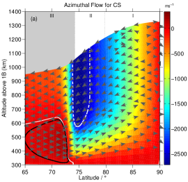
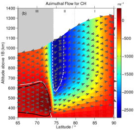
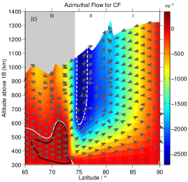
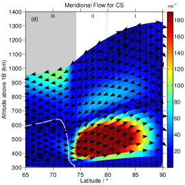
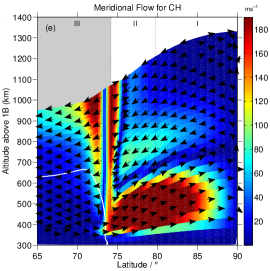
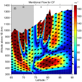
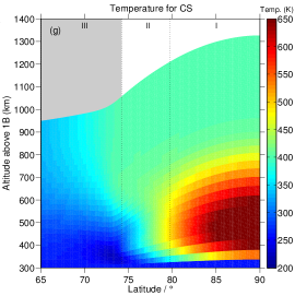
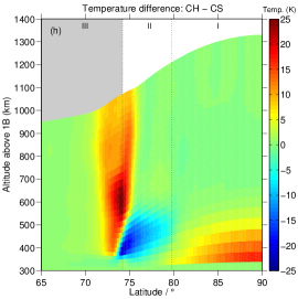
Figure 4: (a)-(c) show the variation of thermospheric azimuthal velocity (colour scale) in the corotating reference frame for cases CS-CF respectively (left to right). Positive values (dark red) indicate super-corotation, whilst negative values (light red to blue) indicate sub-corotation. The arrows show the direction of meridional flow and the solid white line indicates the locus of rigid corotation. The solid black encloses regions of super-corotation ($>25\,\mathrm{m\,s^{-1}}$) and the dashed white line encloses regions that are sub-corotating at a rate $<-2500\,\mathrm{m\,s^{-1}}$. The magnetospheric regions (region III is shaded) are separated by dotted black lines and labelled. (d)-(f) show the meridional velocity in the thermosphere for cases CS-CF. The colour scale indicates the speed of flows. All other labels and are as for (a)-(c). (g) shows the thermospheric temperature distributions for case CS whilst (h)-(i) show the temperature difference of cases CH and CF with case CS. The white contour encloses temperature differences $>100\,\mathrm{K}$. All labels are as in (a)-(c).

Figs. 4a-c show the variation of thermospheric azimuthal velocity (in the corotating reference frame) in the high latitude thermosphere for cases CS-CF respectively. Positive (resp. negative) values of azimuthal velocity indicate super (resp. sub)-corotating regions. The direction of meridional flow is indicated by the black arrows, the locus of rigid corotation is indicated by the solid white line, strong super-corotation ($<25\,\mathrm{m\,s^{-1}}$) is indicated by the black contour, strong sub-corotation ($>-2500\,\mathrm{m\,s^{-1}}$) is indicated by the dashed white contour. Magnetospheric regions are labelled and separated by black dotted lines. Zonally, there are two prominent features in our transient compression cases:

i) a low altitude small super-corotating jet, centred at ${\sim}72\,\mathrm{{}^{\circ}}$. In case CS, this jet is created by a small excess in the zonal Coriolis and advection momentum terms compared to the ion drag term. At low altitude, the Coriolis force is primarily directed eastwards and unopposed can promote super-corotation in the neutrals (Smith and Aylward, 2009; Yates et al., 2012).

ii) a large sub-corotating jet, from region III - I (blue region in Figs. 4a-c). This sub-corotational jet is caused by the drag of the sub-corotating magnetosphere on the thermosphere. Zonal flows in this region are generally sub-corotational and acceleration terms are balanced in case CS, as the thermosphere is in steady-state.

Figs. 4d-f shows the variation of meridional flows in the high latitude thermosphere for our transient compression cases. Magnetospheric labels, locus of corotation and arrows are the same as in Figs. 4a-c. These figures show the meridional flow patterns in the thermosphere, as well as localised accelerated regions (red/brown hues). In steady state, flow patterns are as described by Smith et al. (2007), Smith and Aylward (2009) and Yates et al. (2012) - where at:

i) Low-altitude (${<}600\,\mathrm{km}$), ion drag acceleration becomes strong due to the Pedersen conductivity layer (maximum value of $0.1163\,\mathrm{mho\,m^{-1}}$ at ${\sim}370\,\mathrm{km}$). An imbalance is created between ion drag, Coriolis and pressure gradient terms; thus, giving rise to advection of momentum, which restores equilibrium in this low altitude region. This results in mostly sub-corotational, poleward accelerated flow as shown by the black arrows and brown hues in Fig. 4d.

ii) High-altitude (${>}600\,\mathrm{km}$), conditions are quite different, meridional Coriolis and pressure gradient accelerations are essentially balanced, whilst terms such as ion drag, advection and zonal Coriolis are small and insignificant. This creates a ‘jovistrophic’ condition, whereby flow is directed very slightly equatorwards and is sub-corotational (see black arrows in Fig. 4d).

The above descriptions of zonal and meridional flow patterns pertain to steady state conditions (Figs. 4a and d respectively). Zonal flows for case CH (Fig. 4b) show little change from the steady state zonal flow patterns described above. The main differences lie in the magnitude of the velocities; velocity in the super-corotational jet doubles and the magnitude of azimuthal velocity has decreased by ${\sim}4\,{\%}$ in the sub-corotational jet. Meridional flows in Fig. 4e show two additional local acceleration regions either side of ${\sim}73\,\mathrm{{}^{\circ}}$ latitude and from altitudes ${>}500\,\mathrm{km}$.

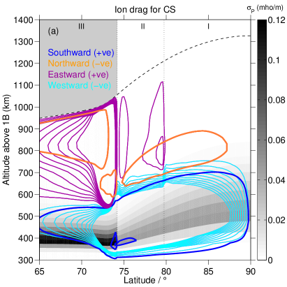
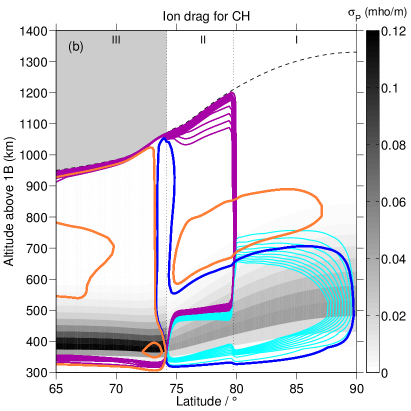
Figure 9: (a) Shows the variation of zonal and meridional ion drag momentum with altitude, latitude and Pedersen conductivity (colour bar) for case CS. The meridional contours (blue and orange) range from $1-500\,\mathrm{mm\,s^{-2}}$ with an interval of $50\,\mathrm{mm\,s^{-2}}$ and with blue being positive (southward) and orange being negative (northward). The zonal contours (purple and cyan) range from $1-10\,\mathrm{mm\,s^{-2}}$ with an interval of $1\,\mathrm{mm\,s^{-2}}$ and with purple being positive (eastwards) and cyan being negative (westwards). The magnetospheric regions are separated and labelled. (b) Variation of zonal and meridional ion drag momentum with altitude, latitude and Pedersen conductivity (colour bar) for case CH. All line styles and labels are as in (a).

In addition, low altitude flow in region III is now directed purely equatorward. This is in marked contrast to the steady state flow patterns. All the changes in flows discussed for case CH result from the super-corotation of the magnetosphere which causes a reversal in the coupling current, subsequently leading to a change in the sign of ion drag momentum terms in region III (see Fig. 9 and corresponding discussion).

Zonal and meridional flows of case CF are respectively show in Fig. 4c and f. The overall flow patterns are as described above for case CH: i) a large sub-corotational jet combined with low altitude poleward flows and high altitude equatorward flows in regions II and I, and ii) a low small low altitude super-corotational jet combined with equatorward flows in region III. However, the degree and spatial extent of super-corotation has decreased and a number of local accelerated regions exist where the direction of meridional flow changes on relatively small spatial scales. These complex flow patterns result from the highly perturbed nature of the case CF thermosphere and the imbalance between ion drag, Coriolis, pressure gradients and advection of momentum terms.

4.3 Thermospheric heating

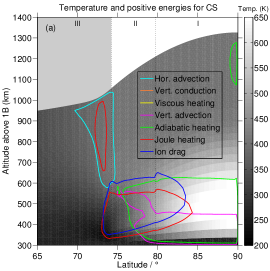
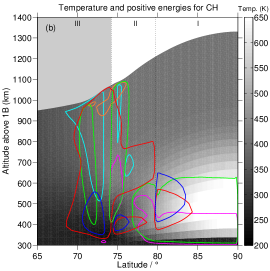
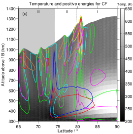
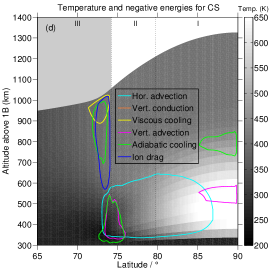
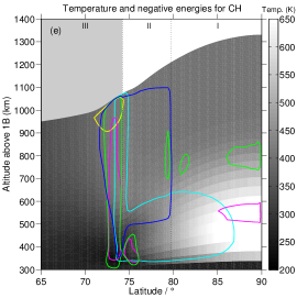
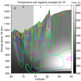
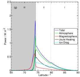
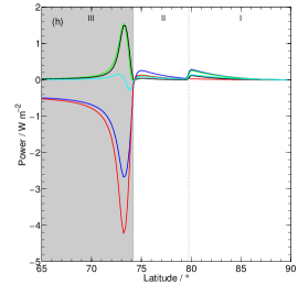
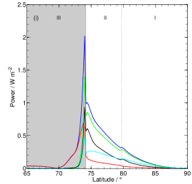
Figure 5: (a)-(c) shows the variation of atmospheric heating terms with altitude, latitude and temperature (colour bar) for cases CS, CH and CF (left to right). The contours enclose regions where heating/kinetic energy rates exceed $20\,\mathrm{W\,kg^{-1}}$. Ion drag energy, Joule heating, vertical and horizontal advection of energy, adiabatic heating/cooling, viscous heating and heat conduction (vertical and turbulent) are represented by blue, red, yellow and magenta, green, cyan and orange lines. The magnetospheric regions are separated and labelled. (d)-(f) show the variation of atmospheric cooling terms where the contours enclose regions where heating/kinetic energy are decreasing (cooling) with rates exceeding $20\,\mathrm{W\,kg^{-1}}$. All colours and labels are as in (a)-(c). (g)-(i) show how the power per unit area varies for our transient compression cases. The blue line represents total power which is the sum of magnetospheric power (red line) and atmospheric power (green line); atmospheric power is the sum of both Joule heating (black solid line) and ion drag energy (cyan solid line). Other labels are as for (a)-(c).

Fig. 4g shows thermospheric temperature as a function of altitude and latitude for case CS. Figs. 4h-i show the difference in thermospheric temperature between cases CH and CS, and cases CF and CS. We will use Figs. 5a-f, showing contour plots for various thermospheric heating (Figs. 5a-c) and cooling (Figs. 5d-f) terms (see plot legends for details) to interpret the temperature response.

In Fig. 4g we see a clear temperature difference between upper (${>}75\,\mathrm{{}^{\circ}}$) and lower (${<}75\,\mathrm{{}^{\circ}}$) latitudes; lower latitudes are cooled whilst upper latitudes are significantly heated (Smith et al., 2007; Smith and Aylward, 2009). We see a ‘hotspot’ (in region I) with a peak temperature of ${\sim}705\,\mathrm{K}$. This arises from the poleward transport of Joule heating (from regions III and II) by the accelerated meridional flows shown in Fig. 4d (Smith and Aylward, 2009; Yates et al., 2012).

Fig. 4h shows the temperature difference between cases CH and CS. There are three prominent features in Fig. 4h:

i) Temperature increase up to ${\sim}26\,\mathrm{K}$ across the region III/II boundary (${z}{\geq}400\,\mathrm{km}$) resulting from a large ($\times 2\,{}$) increase in Joule heating and the addition of other heat sources, such as adiabatic heating (see Fig. 5b). The large increase in Joule heating is caused by the increase in the rest-frame electric field, and the corresponding Pedersen current density.

ii) Temperature decrease down to ${\sim}{-}22\,\mathrm{K}$, at low altitudes of region II. Fig. 5b shows that at low altitudes (${\leq}500\,\mathrm{km}$) of region II there is, on average, a $20\,{\%}$ decrease in energy dissipated by Joule heating and ion drag energy. This, coupled with the presence of energy lost by ion drag energy (Fig. 5e) in this region causes the significant decrease in temperature shown above. All the factors discussed above result from the reversal and decrease (in magnitude) of the flow shear between the magnetosphere and thermosphere in case CH.

iii) A maximum of ${\sim}17\,\mathrm{K}$ increase at low altitudes in region I. The meridional velocity of case CH increases slightly (${\sim}2\,\mathrm{\%}$) in this region and, as such, can transport heat from Joule heating and ion drag energy polewards somewhat more efficiently than in case CS.

Fig. 4i shows the temperature difference between cases CF and CS. Immediately, we can see that there are changes in the distribution of temperature in the upper thermosphere of case CF. There are four ‘finger-like’ regions with local temperature increases ${\geq}50\,\mathrm{K}$ (maximum of $175\,\mathrm{K}$; white contour encircles regions where temperature difference is ${\geq}100\,\mathrm{K}$) and three regions with temperature decreases ${\leq}40\,\mathrm{K}$. These alternating temperature deviations increase with altitude and are collocated with accelerated meridional flow regions. Considering Figs. 5c and f, we see that the heating and cooling terms are now quite complex, with advective and adiabatic terms dominating (${\geq}10\,\mathrm{\times}$ Joule heating and ion drag energy terms). The CF thermosphere appears to be transporting heat, both equatorward and poleward from the region III/II boundary (see Fig. 4f). Achilleos et al. (1998) also shows a similar phenomenon (see top left of Fig. 9 in Achilleos et al. (1998)), whereby perturbations of high temperature are transported away from the auroral region by meridional winds. The energy deposited in the auroral regions heats the local thermosphere which increases local pressure gradients. Advection then attempts to redistribute this heat which momentarily cools the local area until enough heat is deposited again and the process restarts.

Figs. 5g-i show powers per unit area as functions of ionospheric latitude for cases CS, CH and CF, respectively (calculated using Eqs. (11 - 15)). Blue lines represent total power transferred to the ionosphere from planetary rotation which is divided into the power used to accelerate the magnetospheric plasma (magnetospheric power; red lines) and power dissipated in the thermosphere (for atmospheric heating and changing kinetic energy; green lines). Atmospheric power is subdivided into Joule heating (black lines) and ion drag energy (cyan lines). In case CS, magnetospheric power is dominant up to ${\sim}73\,\mathrm{{}^{\circ}}$, where atmospheric power quickly dominates for all poleward latitudes (see Fig. 5g). This indicates that a relatively expanded M-I system (in steady-state) generally dissipates more heat in the atmosphere than in acceleration of outward-moving plasma (Yates et al., 2012). In case CF, powers per unit area closely resemble those for case CS. There are increases in peak magnetospheric power (${\sim}10\,\mathrm{\%}$) and Joule heating (${\sim}25\,\mathrm{\%}$) leading to an overall maximum increase in available power of ${\sim}10\,\mathrm{\%}$. This increase in total power is ultimately due to the lag in response of the thermosphere. For case CH, Fig. 5h, we see the effects of plasma super-corotation in region III, where magnetospheric power reverses (now negative) and energy is now transferred from magnetosphere to thermosphere. As a consequence, heat dissipated as Joule heating doubles, positive ion drag energy decreases by ${\sim}70\,\mathrm{\%}$ and negative ion drag energy increases by two orders of magnitude. These effects lead to the local temperature variations seen above. Powers decrease in region II due to the decrease in azimuthal flow shear between the magnetosphere and thermosphere (see Fig. 2a).

5 Magnetospheric Expansions

This section presents our findings for a transient magnetospheric expansion event with a three hour duration.

5.1 Auroral currents

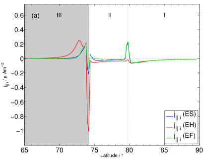
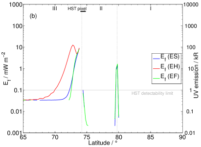
Figure 6: (a) FAC densities in the high latitude ionospheric region for our transient expansion cases. The blue line represents case ES whilst the red and green lines indicate cases EH and EF respectively. The conjugate magnetospheric regions (region III is shaded) are separated by dotted black lines and labelled. (b) Shows the latitudinal variation of the precipitating electron flux (on the left axis) and the corresponding UV auroral emission (on the right axis) for the transient expansion cases. The colour codes and in plot labels are the same as (a). The latitudinal size of an ACS-SBC HST pixel located near the main auroral emission is represented by the dark grey box. The solid grey line indicates the limit of detectability of the HST (Cowley et al., 2007).

FAC densities in the high latitude region are plotted for cases ES (blue line), EH (red line) and EF (green line) in Fig. 6. Comparing cases ES with EH we see three main differences: i) EH has two upward FACs peaks in region III (of similar magnitude to the peak in case ES) creating a large area of upward-directed FAC, ii) the magnitude of downward FAC near the region III boundary has increased by a factor of four (from ES to EH) and iii) FAC densities at the region II/I boundary are entirely downward-directed, unlike case ES. As the magnetosphere expands, its magnetic field strength and plasma angular velocity decrease. This change in ${\Omega_{M}}$ (see Fig. 2b) increases the flow shear between the magnetosphere and thermosphere and thus increases the FAC density in region III by ${\sim}15\,\mathrm{\%}$. The strong downward FAC results from the large gradients in ${\Omega_{M}}$ through the poleward boundary of region III, where magnetodisc plasma moves from a region with angular velocity of ${~{}}0.9\,\mathrm{\Omega_{J}}$ to a region moving at ${~{}}0.2\,\mathrm{\Omega_{J}}$. The lack of a peak at the region II/I boundary is due to the small change in ${\Omega_{M}}$ as the model traverses these two regions. Case EF shows only small differences with case ES due to the lag in response time of the thermosphere to transient magnetospheric changes on this time scale.

Looking now at case EH, and comparing FAC densities with the corresponding result from Cowley et al. (2007) (expansion from $45{-}85\,\mathrm{R_{J}}$), we notice a few differences: i) the magnitude of peak upward FAC in case EH is ${\sim}25\,\mathrm{\%}$ larger than that in Cowley et al. (2007) and, ii) case EF has no upward FAC at the region II/I boundary, contrary to results in Cowley et al. (2007). These differences emphasise the effect of using a time-dependent GCM for the thermospheric response. For example, the ‘double peak’ structure in the upward Region III FACs is due to additional modulation of current density by thermospheric flow.

We interpret our FAC density profiles by considering the corresponding precipitating electron energy fluxes, shown in Fig. 6b. Fluxes are plotted as functions of latitude. The line style code and labels are the same as in Fig. 6a, the latitudinal size of a HST ACS-SBC pixel is indicated by the dark grey rectangle and the grey solid line indicates the limit of present HST detectability (${\sim}1\,\mathrm{kR}$; Cowley et al. (2007)). We begin by comparing profiles for case ES with EF, which are almost identical and both have maxima at ${\sim}74\,\mathrm{{}^{\circ}}$ latitude, equivalent to the location of the ‘main auroral oval’, and at ${\sim}80\,\mathrm{{}^{\circ}}$, the boundary between open (region I) and closed field lines (region II). Therefore, we would expect a fairly bright auroral oval of ${\sim}88\,\mathrm{kR}$ for case ES and ${\sim}79\,\mathrm{kR}$ for case EF. The electron energy flux for case EF (${\sim}7.85\,\mathrm{mW\,m^{-2}}$) is ${\sim}10\,\mathrm{\%}$ smaller than case ES (${\sim}8.8\,\mathrm{mW\,m^{-2}}$) due to ${\Omega_{T}(ES)}{>}{\Omega_{T}(EF)}$ leading to a smaller flow shear. Our model also predicts the possibility of observable polar emission (region II/I boundary) of ${\sim}15\,\mathrm{kR}$ for both cases ES and EF. However, this region is strongly dependent on the plasma flow model used and poorly constrained by observations.

Energy flux ${E_{f}}$ for case EH is non-existent, poleward of ${\sim}74\,\mathrm{{}^{\circ}}$ latitude, due to the downward (negative) FAC density in this region. In region III, there are two upward FAC peaks, separated by ${\sim}1\,\mathrm{{}^{\circ}}$. The first one, located at ${\sim}73\,\mathrm{{}^{\circ}}$ is ${\sim}37\,\mathrm{\%}$ larger than the second, at ${\sim}74\,\mathrm{{}^{\circ}}$. These peaks result from the large degree of magnetospheric sub-corotation and the modulation of the thermospheric angular velocity in region III (evident in Fig. 2b). Comparing case EH with the equivalent expansion case in Cowley et al. (2007); case EH, in region III, has a maximum value of ${E_{f}}$ (${\sim}12.6\,\mathrm{mW\,m^{-2}}$) that is twice that in Cowley et al. (2007). This study represents the thermosphere with a GCM which responds self-consistently to time-dependent changes in ${\Omega_{M}}$ profiles. Our results indicate that this response is not as strong as that in Cowley et al. (2007), who use a simple ‘slippage’ relation to model the thermospheric angular velocity. At the open-closed field line (region II/I) boundary, Cowley et al. (2007) obtain larger energy fluxes due to their large change in ${\Omega_{M}}$ across these regions; in our study, we obtain negligible changes in ${E_{f}}$ due to our smaller change in imposed ${\Omega_{M}}$ across this boundary.

5.2 Thermospheric dynamics

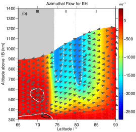
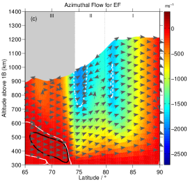
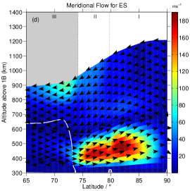
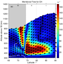
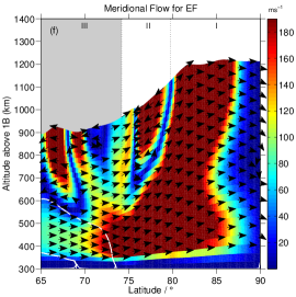
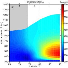
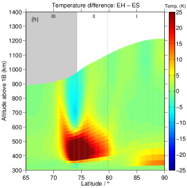
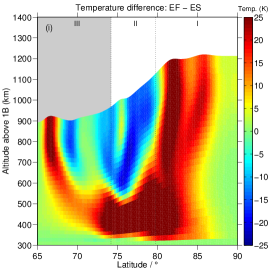
Figure 7: (a)-(c) show the variation of thermospheric azimuthal velocity (colour scale) in the corotating reference frame for cases ES-EF respectively (left to right). Positive values (dark red) indicate super-corotation, whilst negative values (light red to blue) indicate sub-corotation. The arrows show the direction of meridional flow and the white line indicates the locus of rigid corotation. The solid black encloses regions of super-corotation ($>25\,\mathrm{m\,s^{-1}}$) and the dashed white line encloses regions that are sub-corotating at a rate $<-1750\,\mathrm{m\,s^{-1}}$. The magnetospheric regions (region III is shaded) are separated by dotted black lines and labelled. (d)-(f) show the meridional velocity in the thermosphere for cases ES-EF. The colour scale indicates the speed of flows. All other labels and are as for (a)-(c). (g) shows the thermospheric temperature distributions for case ES whilst (h)-(i) show the temperature difference between cases EH and EF and case ES. All labels are as in (a)-(c).

The altitude-latitude variation of azimuthal and meridional thermospheric velocities and temperature are shown in Fig. 7. The first column in Fig. 7 shows thermospheric outputs for case ES; cases EH and EF are represented in columns two and three respectively.

For case ES, the zonal (Fig. 7a) and meridional (Fig. 7d) flows are very similar to those discussed in Yates et al. (2012) as the only difference between both steady-state compressed cases is that here we assume a constant height-integrated Pedersen conductivity whilst in Yates et al. (2012) the conductivity is enhanced by FAC. Zonal flows show a low-altitude super-corotational jet in region III and two sub-corotational jets across regions II and I. The meridional flows show the previously discussed flow patterns i.e. low-altitude poleward flow and high-altitude equatorward flow.

Thermospheric flows for case EH are slightly different from those of case ES. A magnetospheric expansion decreases the degree of plasma corotation which subsequently decreases the thermospheric zonal velocities i.e. they become more sub-corotational (see Fig. 7b). In the meridional sense (Fig. 7e), low altitude flows remain poleward but with an increased magnitude (up to ${\sim}30\,\mathrm{\%}$) and all flow in region II is now directed poleward. Extra heating (see section 5.3) near the region III/II boundary causes the forces in the local thermosphere to become unbalanced leading to accelerated flows in the poleward and equatorward (high-altitude of region III) directions.

The thermospheric velocities at the end of the transient expansion event (case EF) are shown in the third column of Fig. 7. We see that the only change in zonal flow patterns is a slight increase in the zonal velocity (algebraic increase). The meridional winds show a large poleward accelerated flow originating at low altitudes in region III and reaching the high altitudes of region I. Two smaller regions of accelerated equatorward flow arise in the upper altitudes of regions III and II. As the magnetosphere returns to its initial configuration, it weakly super-corotates over most of region III; this transfers angular momentum to the sub-corotating thermosphere which acts to ‘spin up’ the thermospheric gas.

5.3 Thermospheric heating

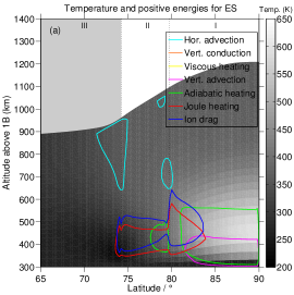
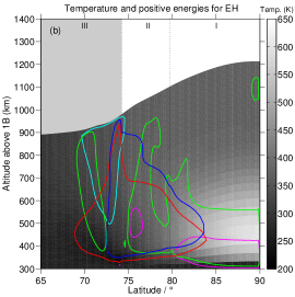
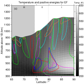
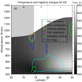
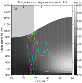
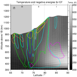
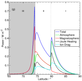
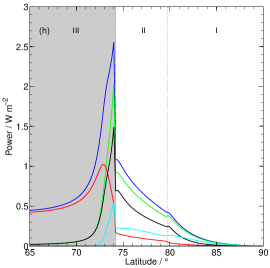
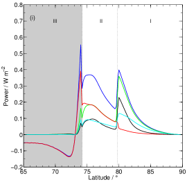
Figure 8: (a)-(c) shows the variation of atmospheric heating terms with altitude, latitude and temperature (colour bar) for cases ES, EH and EF (left to right). The contours enclose regions where heating/kinetic energy rates exceed $20\,\mathrm{W\,kg^{-1}}$. Ion drag energy, Joule heating, vertical and horizontal advection of energy, adiabatic heating/cooling, viscous heating and heat conduction (vertical and turbulent) are represented by blue, red, yellow and magenta, green, cyan and orange lines. The magnetospheric regions are separated and labelled. (d)-(f) show the variation of atmospheric cooling terms where the contours enclose regions where heating/kinetic energy are decreasing (cooling) with rates exceeding $20\,\mathrm{W\,kg^{-1}}$. All colours and labels are as in (a)-(c). (g)-(i) show how the power per unit area varies for our transient expansion cases. The blue line represents total power which is the sum of magnetospheric power (red line) and atmospheric power (green line); atmospheric power is the sum of both Joule heating (black solid line) and ion drag energy (cyan solid line). All other labels are as for (a)-(c).

Fig. 7g shows temperature as a function of altitude and latitude for case ES. Figs. 7h-i show the difference in thermospheric temperature between cases EH and ES, and cases EF and ES, as functions of altitude and latitude. Magnetospheric regions are labelled and separated by black dotted lines and temperatures are indicated by the colour bar. Interpretation of the response of thermospheric temperature is aided by Figs. 8a-f, showing contour plots for various thermospheric heating (Figs. 8a-c) and cooling (Figs. 8d-f) terms (see plot legends for details).

Fig. 7g shows similar results to those described in section 4.3. The main difference is related to the polar ‘hotspot’ which is considerably cooler (peak temperature of ${\sim}590\,\mathrm{K}$) than that for case CS (peak temperature ${\sim}705\,\mathrm{K}$). As previously discussed, the ‘hotspot’ results from the meridional transport (via poleward accelerated flows) of Joule heating from lower latitudes (${\sim}73{-}84\,\mathrm{{}^{\circ}}$; see Figs. 7d and 8a) (Smith and Aylward, 2009; Yates et al., 2012).

Fig. 7h exhibits the temperature difference between cases EH and ES. The figure shows a maximum of ${\sim}50\,\mathrm{K}$ temperature increase at low altitudes (${<}700\,\mathrm{km}$) in regions III and II. Also evident are two minor temperature variations: i) ${\sim}10\,\mathrm{K}$ decrease at high altitude, centred on the region III/II boundary and, ii) ${\sim}10\,\mathrm{K}$ increase in the polar ‘hotspot’ region. Fig. 8b shows a large (${\geq}4{\times}\,\mathrm{}$) increase in ion drag energy and Joule heating rates which accounts for the temperature increase across regions III and II. This low-altitude increase in temperature causes a local increase in pressure gradients leading to accelerated meridional flows being able to efficiently transport heat away from the region III/II boundary and towards the pole. The high altitude cool region ensues from local equatorward and poleward meridional flows combined with factor-of-three increase in adiabatic cooling (Fig. 8e).

Fig. 7i shows the temperature difference between cases EF and ES. The temperature profile has changed significantly from that in Fig. 7h. There are two regions where temperatures increase by up to ${\sim}50\,\mathrm{K}$: i) extending from ${\sim}73{-}85\,\mathrm{{}^{\circ}}$ latitude and low altitudes in regions III and II, and all altitudes in region I (these map to the large poleward-accelerated region in Fig. 7f); and ii) high-altitude (${>}600\,\mathrm{km}$) region, centred at ${\sim}66\,\mathrm{{}^{\circ}}$ latitude. These regions are primarily heated by horizontal advection (high-altitude only) and adiabatic terms (all altitudes) as shown in Fig. 8c; these heating rates have increased (from case ES) by, at most, $800\,\mathrm{\%}$ and $500\,\mathrm{\%}$ respectively. The final feature of note in Fig. 7i is the region cooled by up to ${\sim}{-}22\,\mathrm{K}$, lying between the two heated regions at altitudes ${>}550\,\mathrm{km}$. This cooling is caused by a combination of local increases in horizontal advection and adiabatic cooling, by factors of three and greater. Similar to case CF, case EF’s meridional flows seem to be transporting heat equatorward and poleward, although the majority of these flows act to transport thermal energy poleward.

Figs. 8g-i show powers per unit area as functions of ionospheric latitude for cases ES-EF respectively. Colour codes and labels are as in Figs. 5g-i. Fig. 8g shows the energy balance in the thermosphere for case ES. As discussed in Yates et al. (2012), most of the energy in region III is expended in accelerating magnetospheric plasma; in region II we have a situation where magnetospheric power and atmospheric power (the sum of Joule heating and ion drag energy) are equal, due to ${\Omega_{M}}{=}0.5\,\mathrm{\Omega_{J}}$. Atmospheric power is dominant in region I. For case EH (Fig. 8h), the magnetodisc plasma sub-corotates to a large degree which causes the majority of available power to be used in accelerating the sub-corotaing plasma. Poleward of ${\sim}73\,\mathrm{{}^{\circ}}$ latitude, the large flow shear (${\Omega_{T}}-{\Omega_{M}}$) leads to an increase in energy dissipated within the thermosphere, primarily through Joule heating. The magnetosphere of case EF super-corotates, compared to the thermosphere, at latitudes ${\leq}73\,\mathrm{{}^{\circ}}$. This causes a reversal in energy transfer, which now flows from magnetosphere to atmosphere and acts to spin up the sub-corotaing neutral thermosphere (see Fig. 8i). Polewards of $73\,\mathrm{{}^{\circ}}$, the energy balance is similar to that of case ES.

6 Discussion

6.1 Effect of a non-responsive thermosphere on M-I coupling currents

Our work makes no a priori assumptions regarding the response of the thermosphere to magnetospheric forcing. The GCM responds self-consistently by solving the Navier-Stokes equations for momentum, energy and continuity. For completeness, we calculated M-I coupling currents for the case of a non-responsive thermosphere (Gong, 2005). To do this, we assume that ${\Omega_{T}}{=}{\Omega_{T}}(CS)$ throughout the entire transient event. In this non-responsive thermosphere scenario, there is an average increase in M-I currents of ${\sim}20\,\mathrm{\%}$ midway through the pulse compared to case CH (obtained using GCM). At full-pulse, however, the non-responsive case has M-I currents that are on average ${\sim}12\,\mathrm{\%}$ smaller than currents in case CF. These differences between a non-responsive thermosphere and a responsive one (GCM), are related to the flow shear between thermosphere and magnetosphere; which, is maximal (resp. minimal) at half-pulse (resp. full-pulse) when using a non-responsive thermosphere. A similar analysis for the expansion scenario results in an average of ${\sim}20\,\mathrm{\%}$ increase in the maximum magnitude of M-I currents in a non-responsive thermosphere, compared to the GCM thermosphere. Here, ${\Omega_{T}}(ES)$ is uniformly larger than ${\Omega_{T}}$ for cases EH and EF (see Fig. 2) so the flow shear in the non-responsive scenario will always be greater than the flow shear obtained with the GCM thermosphere.

6.2 The auroral response: predictions and comparisons with observations

Figs. 3b and 6b respectively show the change in precipitating electron energy flux in response to transient magnetospheric compression and expansion events. We also indicate (on the right axis of these Figures) the corresponding UV emission associated with such energy fluxes (assuming that $1\,\mathrm{mW\,m^{-2}}$ of precipitation creates ${\sim}10\,\mathrm{kR}$ of UV output). Considering the compression scenario, our results suggest that the arrival of a solar wind shock would increase the UV emission of the main oval from ${\sim}600\,\mathrm{kR}$ to ${\sim}2800\,\mathrm{kR}$ (factor of $4.7\,\mathrm{}$) and constrict the width of the oval by ${\sim}0.2\,\mathrm{{}^{\circ}}$. The HST detectability limit and the size of an HST pixel (dark grey box in Fig. 3b) suggest that such an increase in auroral emission would be detectable but the constriction of the main oval may be too small to be observed. Clarke et al. (2009) and Nichols et al. (2009) observed that the brightness of UV auroral emission increased by a factor of two, in response to transient (almost instantaneous) increases in solar wind dynamic pressure (${\sim}0.01{-}0.3\,\mathrm{nPa}$ or equivalently ${\sim}109{-}72\,\mathrm{R_{J}}$). The increase in UV emission was also found to persist for a few days following the solar wind shock. Nichols et al. (2009) also observed poleward shifts (constrictions) in main oval emission on the order of ${\sim}1\,\mathrm{{}^{\circ}}$ corresponding to the arrival of solar wind shocks.

Total emitted UV power may also be used to describe auroral activity, assuming that this quantity is ${\sim}10\,\mathrm{\%}$ of the integrated electron energy flux per hemisphere (Cowley et al., 2007). Case CH has a total UV power of ${\sim}1.58\,\mathrm{TW}$ (compared to ${\sim}420\,\mathrm{GW}$ for case CS), which is a factor of two to three times larger than UV powers observed by both Clarke et al. (2009) and Nichols et al. (2009). The profile of case CH also indicates the possibility of observable polar emission at region II/I (open-closed) boundary. This conclusion is, however, sensitive to our model assumptions (see section 6.4).

Our model results predict very different behaviour for the expansion scenario (Fig. 6b). At maximum expansion we would expect a small increase (${\sim}40\,\mathrm{kR}$) in peak main oval brightness along with a ${\sim}1\,\mathrm{{}^{\circ}}$ equatorward shift (expansion) of the oval. We also note the possible observation of a somewhat bifurcated main oval (see HST pixel in Figure); with emission peaking at ${\sim}73\,\mathrm{{}^{\circ}}$ and ${\sim}74\,\mathrm{{}^{\circ}}$ latitude. The main oval would, either way, appear considerably broader (${\sim}2{-}3\,\mathrm{{}^{\circ}}$) as a result of the large increase in the spatial region of magnetospheric sub-corotation. Clarke et al. (2009) observed little change in auroral brightness near the arrival of a solar wind rarefaction region, however Nichols et al. (2009) have seen changes in main oval location. The total UV power in case EH is ${\sim}270\,\mathrm{GW}$ (compared to ${\sim}78\,\mathrm{GW}$ in case ES). While this power is considerably smaller than that in case CH, it is comparable to UV powers calculated in Clarke et al. (2009) and Nichols et al. (2009), following solar wind rarefactions (${\sim}200-400\,\mathrm{GW}$).

6.3 Global thermospheric response

The arrival of solar wind shocks or rarefactions has, for the most part, a similar effect on thermospheric flows. Our modelling shows a general increase (resp. decrease) in the degree of corotation with solar wind dynamic pressure increases (resp. decreases). Zonal flow patterns remain essentially unchanged with a large sub-corotational jet and a small super-corotational jet. Meridional flow cells however, respond to transient magnetospheric reconfigurations somewhat chaotically, with numerous poleward and equatorward accelerated flow regions developing (at altitudes $>600\,\mathrm{km}$) with time throughout the event. The overall low-altitude poleward flow remains fixed with solar wind rarefactions but reverses in response to a solar wind shock (see cases CH and CF in Figs. 4e and f). This flow becomes equatorward due to a reversal in the direction of ion drag acceleration in the region III, as shown in Fig. 9. This reversal, in turn, arises from the super-corotation of magnetospheric plasma.

Compared to the transient compression case CF, the EF thermosphere seems fairly stable i.e. there are no sharp peaks and troughs in the upper boundary. Our interpretation is that for the compression scenario the magnetosphere transfers a large amount of angular momentum to the thermosphere due to its large degree of super-corotation. This surge in momentum and energy input to the thermosphere over a short time scale causes significant strain on the thermosphere and thus requires a drastic reconfiguration in order to attempt to re-establish dynamic equilibrium. On the other hand, in our expansion scenario the magnetosphere significantly sub-corotates for most of the event and only super-corotates compared to the planet and thermosphere (slightly) nearing the end of the event. Thus, for the majority of the expansion event the thermosphere is losing angular momentum to the magnetosphere. This implies that its dynamics and energy input are generally smaller than the transient compression scenario, which leads to a less ‘drastic’ response.

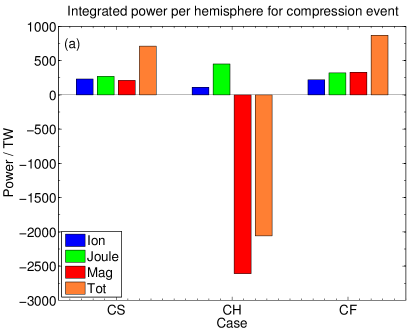
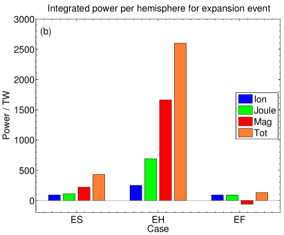
Figure 10: (a) Integrated ionospheric powers per hemisphere for cases CS-CF are represented in this figure. Ion drag energy is represented by blue bars, Joule heating by green bars, magnetospheric power by red bars and total (sum of all above) is represented by orange bars. See text for further detail. (b) Integrated ionospheric powers per hemisphere for cases ES-EF are represented in this figure.

The magnetospheric reconfigurations discussed above have been shown to have a significant impact on the dynamics and energy balance of the thermosphere. We now attempt to globally quantify such changes in energy by calculating the integrated power per hemisphere obtained from the power densities in Figs. 5g-i and 8g-i. These integrated powers are presented in Figs. 10a and b for the compression and expansion scenarios respectively. Blue bars represent the kinetic energy dissipated by ion drag, green bars indicate Joule heating, red bars represent the power used to accelerate magnetospheric plasma and orange bars simply represent the sum of all the above terms. Positive powers indicate energy dissipated in/by the thermosphere whilst negative powers indicate energy deposited into the thermosphere.

Midway through the compression event (case CH), magnetospheric plasma super-corotates compared to the thermosphere and deep atmosphere. This reverses the direction of momentum and energy transfer so that energy is now being transferred from the magnetosphere to the thermosphere. Our results indicate that ${\sim}2000\,\mathrm{TW}$ of total power (magnetospheric, Joule heating and ion drag energy) is gained by the coupled system as a result of plasma super-corotation. Note that this is considerably larger than the ${\sim}325\,\mathrm{TW}$ (closed and open field regions) calculated in Cowley et al. (2007) for a responsive thermosphere scenario. This energy transfer from the magnetosphere would act to, essentially ‘spin up’ the planet (Cowley et al., 2007) and increase the thermospheric temperature. In case CF, plasma is not super-corotating; thus the picture is fairly similar to case CS. The main difference is that there is a ${\sim}20\,\mathrm{\%}$ increase in total power dissipated in the atmosphere and in acceleration of the magnetosphere. This arises from increases in flow shear due to the ‘lagging’ thermosphere (see Fig. 2) and inevitably leads to the local temperature increases seen in Fig. 4i and discussed above. The finite time required for thermospheric response results in the described ‘residual’ perturbations to the initial system (CS) even after the pulse has subsided (CF).

A transient magnetospheric expansion event creates a significant increase in both power dissipated in the atmosphere due to Joule heating (${\sim}6{\times}\,\mathrm{}$ that of ES) and ion drag energy (${\sim}3{\times}\,\mathrm{}$ that of ES). Moreover, the power used to accelerate the magnetosphere towards corotation is ${\sim}7{\times}\,\mathrm{}$ that of ES, and is shown in Fig. 10b. These increases lead to a total power per hemisphere of ${\sim}2600\,\mathrm{TW}$ which is three times larger than the responsive thermosphere case in Cowley et al. (2007). These changes in heating and cooling create the local temperature increases discussed above. For case EF, where we now have the magnetosphere rotating faster than the thermosphere, there is a ${\sim}75\,\mathrm{\%}$ decrease in the magnitude of ‘magnetospheric’ power. The magnetosphere is thus transferring power to the thermosphere in this case, albeit a relatively small amount. This effectively ‘pulls’ the thermosphere along, increasing its angular velocity in order to return to the steady-state situation where ${\Omega_{T}{>}\Omega_{M}}$. We note that energy dissipated via Joule heating also decreases slightly due to the small decrease in flow shear. Overall, then, the total power per hemisphere in case EF is only $30\,\mathrm{\%}$ that of case ES.

Results for cases CH and EH show large (approximately three orders of magnitude larger than solar heating) increases in energy either being deposited or dissipated in the thermosphere. Observations by Stallard et al. (2001, 2002) of an auroral heating event at Jupiter were ananlysed by Melin et al. (2006). These authors found that during this auroral heating event, which they attribute to being caused by a decrease in solar wind dynamic pressure, the combined ion drag energy and Joule heating rates increase from $67\,\mathrm{mW\,m^{-2}}$ to $277\,\mathrm{mW\,m^{-2}}$ over three days. They proposed that this extra heat must then be transported equatorward from the auroral regions by an increase in equatorward meridional winds (Waite et al., 1983). If we assume that their auroral region ranges from $65\,\mathrm{{}^{\circ}}$ to $85\,\mathrm{{}^{\circ}}$ latitude and that these heating rates are constant across such a region, the total energy dissipated by Joule heating and ion drag energy increases from ${\sim}193\,\mathrm{TW}$ to ${\sim}800\,\mathrm{TW}$. This increase is comparable to the increase of Joule heating and ion drag energy in our expansion scenario, going from case ES (${\sim}201\,\mathrm{TW}$) to EH (${\sim}942\,\mathrm{TW}$). Increase in Joule heating and ion drag energy from case CS to CH is more modest (${\sim}499\,\mathrm{TW}$ to ${\sim}555\,\mathrm{TW}$) due to the reversal of kinetic energy exchange between atmospheric neutrals and ions and despite an increase in Joule heating. Our modelling supports the work of Melin et al. (2006) in terms of i) the magnitude of energy dissipated in the thermosphere and ii) the type of magnetospheric reconfiguration required. We do not however, see a significant increase in equatorward flows in our expansion scenario. Our compression scenario, however, shows a large change in meridional flow patterns with a large portion of the thermosphere flowing equatorwards.

6.4 Model limitations

The main limitation to our transient model is the use of a fixed model for relative changes in conductivity with altitude, and a uniform Pedersen conductance ${\Sigma_{P}}$ for the ionosphere (see section 3.2). Whilst not ideal, we feel it is a suitable first step to developing a fully self-consistent, time-dependent model of the Jovian magnetosphere-ionosphere-thermosphere system. Use of an enhanced conductivity model would concentrate all but background levels of conductance just equatorward of the main auroral oval location (${\sim}74\,\mathrm{{}^{\circ}}$) (Yates et al., 2012); effectively increasing the coupling between the atmosphere and magnetosphere in this region. We would thus expect the magnitude of current densities to increase in the region near the main oval (region III/II boundary in our model), along with an increase in the Joule heating rate.

The high conductivity at latitudes between $60\,\mathrm{{}^{\circ}}$ and $70\,\mathrm{{}^{\circ}}$ in the present model, combined with the super-corotation of the thermosphere, allows for the plasma magnetically mapped to these ionospheric latitudes to super-corotate slightly in steady state. With an enhanced conductivity model, this region would have a super-corotating thermosphere but low, background-level conductances (e.g. Smith and Aylward (2009); Yates et al. (2012)). Therefore, even though the super-corotating thermosphere acts to accelerate the magnetodisc plasma, the low conductances inhibit how efficiently the plasma is accelerated. It is worth noting that despite the fact that, in this study, both the neutral thermosphere and magnetodisc plasma super-corotate compared to the deep atmosphere, as long as the plasma sub-corotates compared to the thermosphere, angular momentum and energy will be transferred from the upper atmosphere to the magnetosphere as is expected in steady state. We plan to incorporate enhancements in Pedersen conductance due to auroral precipitation of electrons in a future study.

Other limitations to this model include:

i) Assumption of axial symmetry: Discussions in Smith and Aylward (2009) conclude that the assumption of axial symmetry with respect to the planet’s rotation axis does not significantly alter the thermospheric outputs of our model. They find that axial symmetry leads to modelling errors on the order of ${\sim}20\,\mathrm{\%}$ which are less than, or at least comparable to, errors derived from the various other assumptions and simplifications made in this coupled model.

ii) No development of field-aligned potentials: Our model does not currently include the development of field-aligned potentials, which accelerate electrons from the high latitude magnetosphere into the ionosphere. We simply apply the linear approximation to the Knight relation (see section B) to obtain precipitating electron energy fluxes. Ray et al. (2009) show that significant field-aligned potentials develop at high-latitudes to supply the necessary FACs, and hence angular momentum, demanded by the magnetospheric plasma. By applying the linear approximation to the Knight relation, we assume that the top of the acceleration region is far enough from the planet such that the ratio of the energy gained by a particle traveling through the potential drop to its thermal energy is significantly less than the mirror ratio between top and bottom of the acceleration region. Consequently, possible current saturation effects are ignored, with the field-aligned current density increasing to values beyond those that would result from the entire electron distribution accelerated into the loss cone. The M-I coupling modelling by Ray et al. (2010) also showed that including field-aligned potentials in a self-consistent treatment of the auroral current system alters the electric field mapping between the ionosphere and the magnetosphere, decoupling the ionospheric and magnetospheric flows. Their model did not explicitly include thermospheric flows; however, the presence of field-aligned potentials may also plausibly alter the thermospheric angular velocity.

iii) Fixed plasma angular velocity in the polar cap region (latitudes ${>}80\,\mathrm{{}^{\circ}}$): The plasma angular velocity in the polar cap region ${\Omega_{Mpc}}$ is fixed at a constant value of ${\sim}0.1\,\mathrm{\Omega_{J}}$, in accordance with the formulations in Isbell et al. (1984) which depend in part on the solar wind velocity ${v_{sw}}$. A change in solar wind dynamic pressure ${p_{sw}}$ would generally be accompanied by a corresponding change in ${v_{sw}}$, so when we change the magnetospheric configuration of our model, ${\Omega_{Mpc}}$ should also change depending on the new value of ${v_{sw}}$. If we assume that the solar wind density ${\rho_{sw}}$ remains constant and that ${p_{sw}\approx\rho_{sw}v_{sw}^{2}}$, ${\Omega_{Mpc}(CS)}\approx 0.06\,\mathrm{\Omega_{J}}$ and ${\Omega_{Mpc}(CH)}\approx 0.17\,\mathrm{\Omega_{J}}$. We find the difference between the plasma angular velocities across the open-closed field line boundary with a constant or variable ${\Omega_{Mpc}}$ to be negligible for both compressed and expanded magnetospheres and thus do not expect this to significantly influence the results discussed above.

7 Conclusion

We investigated the effect of transient variations in solar wind dynamic pressure on the M-I coupling currents, thermospheric flows, heating and cooling rates and aurora of the Jovian system. We considered two scenarios: i) a transient compression event, and ii) a transient expansion event. Both of these were imposed over a time scale of three hours. A transient compression event consists of an initially expanded, steady-state magnetospheric configuration. The model Jovian magnetosphere then encounters a shock in the solar wind, which compresses the system. As the conceptual shock propagates past the magnetosphere, a rarefaction region follows and the magnetosphere subsequently expands back to its initial state. The opposite occurs for our expansion event.

We have made an important initial step into investigating how time-dependent phenomena affect the Jovian system. In steady state, the more expanded the magnetosphere is, the hotter Jupiter’s thermosphere is likely to be (Yates et al., 2012). The caveat to this is that only the polar (high-altitude) region of the thermosphere (due to the poleward meridional winds) approaches the observable temperatures of ${\sim}900\,\mathrm{K}$ (Seiff et al., 1998; Yelle and Miller, 2004; Lystrup et al., 2008). The lower latitudes are still relatively cool with temperatures of ${\sim}200-300\,\mathrm{K}$, compared to polar temperatures of up to ${\sim}700\,\mathrm{K}$. On the other hand, when we consider rapid magnetospheric reconfigurations, the situation is quite different. We see a change in the direction of meridional winds as well as a large (at least a factor of two) increase in Joule heating and energy being dissipated in or deposited to the thermosphere. These winds redistribute the extra heat, essentially sending ‘wave-like perturbations’ of high-temperature gas (higher than ambient surroundings) towards both the polar and equatorial regions (Waite et al., 1983; Achilleos et al., 1998; Melin et al., 2006). The present results are not enough to increase the temperature of the equatorial thermosphere to its observed values but we stress that all the results presented herein occur within a period of three hours (approximately ${1/3}$ of a Jovian day). This leads to the potential of future, more realistic, time-dependent studies whereby one could vary the duration of such transient events, experiment with ‘chains’ of such events and/or more realistic solar wind dynamic pressure profiles, in order to model the dynamic response of the Jovian thermosphere over more extended periods of external perturbation.

Table 1: Transient state Pedersen conductances in our model thermosphere. General regions of the thermosphere are indicated in the left column whilst their respective ionospheric latitude is indicated in the middle column. The right column shows the value/profile of the height-integrated Pedersen conductance assumed in each respective region.

Location	Ionospheric latitude / ∘	${\Sigma_{P}}$ / mho	Reference
Equatorial	$<60\,\mathrm{}$	$0.0275\,\mathrm{}$	Hill (1980)
Auroral	$60\,\mathrm{}\leq{\theta}\leq 74\,\mathrm{}$	$0.5\,\mathrm{}$	this work, see also Nichols (2011)
Polar regions	$>74\,\mathrm{}$	$0.2\,\mathrm{}$	Isbell et al. (1984)

Table 2: The three different stages of the transient magnetospheric reconfiguration events (compression and expansion). The radii of the magnetodisc ${R_{MM}}$, magnetopause ${R_{MP}}$ and corresponding solar wind pressure ${P_{SW}}$ (Joy et al., 2002) are shown.

Case	CS	CH	CF	ES	EH	EF
${R_{MM}}$/ $\mathrm{R_{J}}$	$85\,\mathrm{}$	$45\,\mathrm{}$	$85\,\mathrm{}$	$45\,\mathrm{}$	$85\,\mathrm{}$	$45\,\mathrm{}$
${R_{MP}}$/ $\mathrm{R_{J}}$	$101\,\mathrm{}$	$68\,\mathrm{}$	$101\,\mathrm{}$	$68\,\mathrm{}$	$101\,\mathrm{}$	$68\,\mathrm{}$
${P_{SW}}$/ $\mathrm{nPa}$	$0.021\,\mathrm{}$	$0.213\,\mathrm{}$	$0.021\,\mathrm{}$	$0.213\,\mathrm{}$	$0.021\,\mathrm{}$	$0.213\,\mathrm{}$

Appendix A Magnetosphere-ionosphere coupling

In this section we discuss the effect of coupling the magnetosphere and ionosphere together. The meridional electric field in the rest frame of the thermosphere may be written as:

$${E_{\theta}}= {B_{i}\rho_{i}\left(\Omega_{T}-\Omega_{M}\right)},$$ (5)

where ${B_{i}}$ is the magnitude of the (assumed) radial ionospheric magnetic field (${B_{i}}{=}{2B_{J}}$).

The combination of electric field, magnetic field and ion-neutral collisions causes Pedersen currents to flow in the ionosphere, mainly perpendicular to the direction of the planetary magnetic field. These ionospheric currents form part of a larger current circuit which includes the radial current flowing in the magnetodisc and the FAC flowing along the magnetic field lines. The height integrated Pedersen current density ${i_{P}}$ and its azimuthally integrated form ${I_{P}(\theta_{i})}$ are (Cowley et al., 2007; Smith and Aylward, 2009)

$${i_{P}}= {\rho_{i}\Sigma_{P}\left(\Omega_{T}-\Omega_{M}\right)B_{i}},$$ (6)

and

$${I_{P}(\theta_{i})}= {2\pi\rho_{i}^{2}\Sigma_{P}\left(\Omega_{T}-\Omega_{M}\right)B_{i}},$$ (7)

where ${\Omega_{T}}$ is a weighted average, computed over altitude, of the angular velocity of the thermosphere. For a more detailed description of this the reader is referred to Yates et al. (2012) and Smith and Aylward (2009).

The height-integrated radial current density in the magnetodisc is denoted by ${i_{\rho}}$ and can be obtained using Eq. (6) under the assumption of current continuity (zero divergence of current density). We have (Nichols and Cowley, 2004; Smith and Aylward, 2009):

$${\rho_{e}i_{\rho}}= {2\rho_{i}i_{P}},$$ (8)

$${I_{\rho}}= {8\pi\Sigma_{P}F_{e}\left(\Omega_{T}-\Omega_{M}\right)},$$ (9)

where ${I_{\rho}}$ is the azimuthally integrated disc current.

The third and final component of our M-I current circuit is the FAC density. ${j_{||i}(\theta_{i})}$ represents the FAC density at the ionospheric footpoint (at co-latitude ${\theta_{i}}$) of the respective field lines. This current density is obtained from the horizontal divergence of the Pedersen current:

$${j_{||i}(\theta_{i})}= {-\frac{1}{2\pi R_{i}^{2}\sin\theta_{i}}}{\frac{dI_{P}}{d\theta_{i}}},$$ (10)

where the sign of ${j_{||i}(\theta_{i})}$ indicates FAC direction (positive upward from planet). Eq. (10) corresponds to the northern hemisphere, where the magnetic field points radially outward (approximately, in auroral region) (Cowley et al., 2007).

The final aspect of M-I coupling we examine in this study is the energy transfer from planetary rotation to the thermosphere and magnetosphere. The angular momentum transfer to the magnetosphere is used to accelerate magnetospheric plasma towards corotation whilst the energy dissipated within the thermosphere is used for heating and increasing kinetic energy. The total power per unit area of the ionosphere transferred from planetary rotation ${P}$ is the sum of atmospheric power ${P_{A}}$ and magnetospheric power ${P_{M}}$ dissipated per unit area (Hill, 2001). As shown by Smith et al. (2005) atmospheric power consists of two components: (i) Joule heating ${P_{J}}$ and (ii) ion drag power ${P_{D}}$, some of may be viscously dissipated as heat. These power relations are (Cowley et al., 2005):

$${P} ={\Omega_{J}\tau},$$ (11)

$${P_{M}} ={\Omega_{M}\tau},$$ (12)

$${P_{A}} ={(\Omega_{J}-\Omega_{M})\tau},$$ (13)

$${P_{J}} ={(\Omega_{T}-\Omega_{M})\tau},$$ (14)

$${P_{D}} ={(\Omega_{J}-\Omega_{T})\tau},$$ (15)

where

$${\tau} ={\rho_{i}i_{P}B_{i}}$$ (16)

represents the torque exerted by the J${\times}$B force per unit area of the ionosphere.

Appendix B Auroral energies

Once FAC densities have been calculated, we can use the methods of Knight (1973) and Lundin and Sandahl (1978), as presented in Cowley et al. (2007), to calculate the enhanced precipitating electron energy flux ${E_{f}}$:

$${E_{f}} ={\frac{E_{f0}}{2}\left(\left(\frac{j_{||i}}{j_{||i0}}\right)^{2}+1\right)},$$ (17)

where ${E_{f0}}$ is the unaccelerated electron energy flux, ${j_{||i0}}$ is the unaccelerated FAC density (or the maximum current that can be carried by the electrons in the absence of field-aligned potential drops) and ${j_{||i}}$ is the upward (positive) FAC density calculated using Eq. (10). To enable a comparison with similar, earlier studies, we use the same electron population values described in Cowley et al. (2007), which are based on observations by Scudder et al. (1981) and Phillips et al. (1993a, b). These parameters are presented in Table 1.

Table 1: Magnetospheric electron source parameters. This table is adapted from Table 1, Cowley et al. (2007). ${N_{e}}$ represents the electron density, ${W_{th}}$ the electron thermal energy, ${j_{||i0}}$ the unaccelerated current density and ${E_{f0}}$ the unaccelerated energy flux.

Parameter	Open field lines	Outer magnetosphere	Middle magnetosphere
${N_{e}}$ / $\mathrm{cm^{-3}}$	$0.5\,\mathrm{}$	$0.02\,\mathrm{}$	$0.01\,\mathrm{}$
${W_{th}}$ / $\mathrm{keV}$	$0.05\,\mathrm{}$	$0.25\,\mathrm{}$	$2.5\,\mathrm{}$
${j_{||i0}}$ / $\mathrm{\mu A\,m^{-2}}$	$0.095\,\mathrm{}$	$0.0085\,\mathrm{}$	$0.013\,\mathrm{}$
${E_{f0}}$ / $\mathrm{mW\,m^{-2}}$	$0.0095\,\mathrm{}$	$0.0042\,\mathrm{}$	$0.067\,\mathrm{}$

References

- Achilleos et al. (1998) Achilleos, N., Miller, S., Tennyson, J., Aylward, A. D., Mueller-Wodarg, I., Rees, D., 1998. JIM: A time-dependent, three-dimensional model of Jupiter’s thermosphere and ionosphere. J. Geophys. Res. 103, 20089–20112.
- Bougher et al. (2005) Bougher, S. W., Waite, J. H., Majeed, T., Gladstone, G. R., Apr. 2005. Jupiter Thermospheric General Circulation Model (JTGCM): Global structure and dynamics driven by auroral and Joule heating. Journal of Geophysical Research (Planets) 110, 4008.
- Caudal (1986) Caudal, G., Apr. 1986. A self-consistent model of Jupiter’s magnetodisc including the effects of centrifugal force and pressure. J. Geophys. Res.91, 4201–4221.
- Clarke et al. (2009) Clarke, J. T., Nichols, J., Gérard, J.-C., Grodent, D., Hansen, K. C., Kurth, W., Gladstone, G. R., Duval, J., Wannawichian, S., Bunce, E., Cowley, S. W. H., Crary, F., Dougherty, M., Lamy, L., Mitchell, D., Pryor, W., Retherford, K., Stallard, T., Zieger, B., Zarka, P., Cecconi, B., May 2009. Response of Jupiter’s and Saturn’s auroral activity to the solar wind. Journal of Geophysical Research (Space Physics) 114 (A13), 5210.
- Connerney et al. (1998) Connerney, J. E. P., Acuña, M. H., Ness, N. F., Satoh, T., 1998. New models of Jupiter’s magnetic field constrained by the Io flux tube footprint. J. Geophys. Res. 103, 11929–11940.
- Cowley et al. (2005) Cowley, S. W. H., Alexeev, I. I., Belenkaya, E. S., Bunce, E. J., Cottis, C. E., Kalegaev, V. V., Nichols, J. D., Prangé, R., Wilson, F. J., 2005. A simple axisymmetric model of magnetosphere-ionosphere coupling currents in Jupiter’s polar ionosphere. J. Geophys. Res. 110 (A9), 11209–11226.
- Cowley and Bunce (2001) Cowley, S. W. H., Bunce, E. J., 2001. Origin of the main auroral oval in Jupiter’s coupled magnetosphere-ionosphere system. Planet. Space Sci. 49, 1067–1088.
- Cowley and Bunce (2003a) Cowley, S. W. H., Bunce, E. J., 2003a. Modulation of Jovian middle magnetosphere currents and auroral precipitation by solar wind-induced compressions and expansions of the magnetosphere: initial response and steady state. Planet. Space Sci. 51, 31–56.
- Cowley and Bunce (2003b) Cowley, S. W. H., Bunce, E. J., 2003b. Modulation of Jupiter’s main auroral oval emissions by solar wind induced expansions and compressions of the magnetosphere. Planet. Space Sci. 51, 57–79.
- Cowley et al. (2007) Cowley, S. W. H., Nichols, J. D., Andrews, D. J., 2007. Modulation of Jupiter’s plasma flow, polar currents, and auroral precipitation by solar wind-induced compressions and expansions of the magnetosphere: a simple theoretical model. Ann. Geophys. 25, 1433–1463.
- Eviatar and Barbosa (1984) Eviatar, A., Barbosa, D. D., Sep. 1984. Jovian magnetospheric neutral wind and auroral precipitation flux. J. Geophys. Res.89, 7393–7398.
- Gong (2005) Gong, B., Dec. 2005. Variations of Jovian aurora induced by changes in solar wind dynamic pressure. Ph.D. thesis, Rice University.
- Grodent et al. (2001) Grodent, D., Waite, J. H., Gérard, J., 2001. A self-consistent model of the Jovian auroral thermal structure. J. Geophys. Res. 106, 12933–12952.
- Hill (1979) Hill, T. W., 1979. Inertial limit on corotation. J. Geophys. Res. 84, 6554–6558.
- Hill (1980) Hill, T. W., Jan. 1980. Corotation lag in Jupiter’s magnetosphere - Comparison of observation and theory. Science 207, 301.
- Hill (2001) Hill, T. W., 2001. The Jovian auroral oval. J. Geophys. Res. 106, 8101–8108.
- Isbell et al. (1984) Isbell, J., Dessler, A. J., Waite, Jr., J. H., 1984. Magnetospheric energization by interaction between planetary spin and the solar wind. J. Geophys. Res. 89, 10716–10722.
- Joy et al. (2002) Joy, S. P., Kivelson, M. G., Walker, R. J., Khurana, K. K., Russell, C. T., Ogino, T., 2002. Probabilistic models of the Jovian magnetopause and bow shock locations. J. Geophys. Res. 107, 1309–1325.
- Knight (1973) Knight, S., May 1973. Parallel electric fields. Planet. Space Sci.21, 741–750.
- Lundin and Sandahl (1978) Lundin, R., Sandahl, I., Jun. 1978. Some characteristics of the parallel electric field acceleration of electrons over discrete auroral arcs as observed from two rocket flights. In: Halvorsen, T., Battrick, B. (Eds.), European Sounding Rocket, Balloon and Related Research, with Emphasis on Experiments at High Latitudes. Vol. 135 of ESA Special Publication. pp. 125–136.
- Lystrup et al. (2008) Lystrup, M. B., Miller, S., Dello Russo, N., Vervack, Jr., R. J., Stallard, T., Apr. 2008. First Vertical Ion Density Profile in Jupiter’s Auroral Atmosphere: Direct Observations using the Keck II Telescope. ApJ677, 790–797.
- Majeed et al. (2009) Majeed, T., Waite, J. H., Bougher, S. W., Gladstone, G. R., Jul. 2009. Processes of auroral thermal structure at Jupiter: Analysis of multispectral temperature observations with the Jupiter Thermosphere General Circulation Model. Journal of Geophysical Research (Planets) 114, 7005.
- Melin et al. (2006) Melin, H., Miller, S., Stallard, T., Smith, C., Grodent, D., Mar. 2006. Estimated energy balance in the jovian upper atmosphere during an auroral heating event. Icarus 181, 256–265.
- Miller et al. (2000) Miller, S., Achilleos, N., Ballester, G. E., Geballe, T. R., Joseph, R. D., Prangé, R., Rego, D., Stallard, T., Tennyson, J., Trafton, L. M., Waite, Jr., J. H., 2000. The role of H+3 in planetary atmospheres. In: Astronomy, physics and chemistry of H+3. Vol. 358 of Royal Society of London Philosophical Transactions Series A. p. 2485.
- Millward et al. (2005) Millward, G., Miller, S., Stallard, T., Achilleos, N., Aylward, A. D., Jan. 2005. On the dynamics of the jovian ionosphere and thermosphere. Icarus 173, 200–211.
- Müller-Wodarg et al. (2006) Müller-Wodarg, I. C. F., Mendillo, M., Yelle, R. V., Aylward, A. D., Jan. 2006. A global circulation model of Saturn’s thermosphere. Planet. Space Sci.180, 147–160.
- Nichols and Cowley (2004) Nichols, J., Cowley, S., 2004. Magnetosphere-ionosphere coupling currents in Jupiter’s middle magnetosphere: effect of precipitation-induced enhancement of the ionospheric Pedersen conductivity. Ann. Geophys. 22, 1799–1827.
- Nichols (2011) Nichols, J. D., Oct. 2011. Magnetosphere-ionosphere coupling in Jupiter’s middle magnetosphere: Computations including a self-consistent current sheet magnetic field model. Journal of Geophysical Research (Space Physics) 116 (A15), 10232.
- Nichols et al. (2009) Nichols, J. D., Clarke, J. T., Gérard, J. C., Grodent, D., Hansen, K. C., Jun. 2009. Variation of different components of Jupiter’s auroral emission. Journal of Geophysical Research (Space Physics) 114 (A13), 6210.
- Phillips et al. (1993a) Phillips, J. L., Bame, S. J., Barraclough, B. L., McComas, D. J., Forsyth, R. J., Canu, P., Kellogg, P. J., Nov. 1993a. Ulysses plasma electron observations in the Jovian magnetosphere. Planet. Space Sci.41, 877–892.
- Phillips et al. (1993b) Phillips, J. L., Bame, S. J., Thomsen, M. F., Goldstein, B. E., Smith, E. J., Dec. 1993b. ULYSSES plasma observations in the Jovian magnetosheath. J. Geophys. Res.98, 21189.
- Pontius (1997) Pontius, D. H., 1997. Radial mass transport and rotational dynamics. J. Geophys. Res. 102, 7137–7150.
- Ray et al. (2010) Ray, L. C., Ergun, R. E., Delamere, P. A., Bagenal, F., Sep. 2010. Magnetosphere-ionosphere coupling at Jupiter: Effect of field-aligned potentials on angular momentum transport. Journal of Geophysical Research (Space Physics) 115 (A14), 9211.
- Ray et al. (2012) Ray, L. C., Ergun, R. E., Delamere, P. A., Bagenal, F., Jan. 2012. Magnetosphere-ionosphere coupling at Jupiter: A parameter space study. Journal of Geophysical Research (Space Physics) 117 (A16), 1205.
- Ray et al. (2009) Ray, L. C., Su, Y.-J., Ergun, R. E., Delamere, P. A., Bagenal, F., Apr. 2009. Current-voltage relation of a centrifugally confined plasma. Journal of Geophysical Research (Space Physics) 114 (A13), 4214.
- Scudder et al. (1981) Scudder, J. D., Sittler, E. C., Bridge, H. S., Sep. 1981. A survey of the plasma electron environment of Jupiter - A view from Voyager. J. Geophys. Res.86, 8157–8179.
- Seiff et al. (1998) Seiff, A., Kirk, D. B., Knight, T. C. D., Young, R. E., Mihalov, J. D., Young, L. A., Milos, F. S., Schubert, G., Blanchard, R. C., Atkinson, D., 1998. Thermal structure of Jupiter’s atmosphere near the edge of a 5-m hot spot in the north equatorial belt. J. Geophys. Res. 103, 22857–22890.
- Smith and Aylward (2008) Smith, C. G. A., Aylward, A. D., 2008. Coupled rotational dynamics of Saturn’s thermosphere and magnetosphere: a thermospheric modelling study. Ann. Geophys. 26, 1007–1027.
- Smith and Aylward (2009) Smith, C. G. A., Aylward, A. D., 2009. Coupled rotational dynamics of Jupiter’s thermosphere and magnetosphere. Ann. Geophys. 27, 199–230.
- Smith et al. (2007) Smith, C. G. A., Aylward, A. D., Millward, G. H., Miller, S., Moore, L. E., 2007. An unexpected cooling effect in Saturn’s upper atmosphere. Nature 445, 399–401.
- Smith et al. (2005) Smith, C. G. A., Miller, S., Aylward, A. D., 2005. Magnetospheric energy inputs into the upper atmospheres of the giant planets. Ann. Geophys. 23, 1943–1947.