A stabilized finite element method for advection-diffusion equations on surfaces

Abstract

A recently developed Eulerian finite element method is applied to solve advection-diffusion equations posed on hypersurfaces. When transport processes on a surface dominate over diffusion, finite element methods tend to be unstable unless the mesh is sufficiently fine. The paper introduces a stabilized finite element formulation based on the SUPG technique. An error analysis of the method is given. Results of numerical experiments are presented that illustrate the performance of the stabilized method.

1 Introduction

Mathematical models involving partial differential equations posed on hypersurfaces occur in many applications. Often surface equations are coupled with other equations that are formulated in a (fixed) domain which contains the surface. This happens, for example, in common models of multiphase fluids dynamics if one takes so-called surface active agents into account [1]. The surface transport of such surfactants is typically driven by convection and surface diffusion and the relative strength of these two is measured by the dimensionless surface Peclet number $Pe_{s}=\frac{UL}{D_{s}}$. Here $U$ and $L$ denote typical velocity and lenght scales, respectively, and $D_{s}$ is the surface diffusion coefficient. Typical surfactants have surface diffusion coefficients in the range $D_{s}\sim 10^{-3}-10^{-5}~{}cm^{2}/s$ [2], leading to (very) large surface Peclet numbers in many applications. Hence, such applications result in advection-diffusion equations on the surface with dominating advection terms. The surface may evolve in time and be available only implicitly (for example, as a zero level of a level set function).

It is well known that finite element discretization methods for advection-diffusion problems need an additional stabilization mechanism, unless the mesh size is sufficiently small to resolve boundary and internal layers in the solution of the differential equation. For the planar case, this topic has been extensively studied in the literature and a variety of stabilization methods has been developed, see, e.g., [3]. We are, however, not aware of any studies of stable finite element methods for advection-diffusion equations posed on surfaces.

In the past decade the study of numerical methods for PDEs on surfaces has been a rapidly growing research area. The development of finite element methods for solving elliptic equations on surfaces can be traced back to the paper [4], which considers a piecewise polygonal surface and uses a finite element space on a triangulation of this discrete surface. This approach has been further analyzed and extended in several directions, see, e.g., [5] and the references therein. Another approach has been introduced in [6] and builds on the ideas of [7]. The method in that paper applies to cases in which the surface is given implicitly by some level set function and the key idea is to solve the partial differential equation on a narrow band around the surface. Unfitted finite element spaces on this narrow band are used for discretization. Another surface finite element method based on an outer (bulk) mesh has been introduced in [8] and further studied in [9, 10]. The main idea of this method is to use finite element spaces that are induced by triangulations of an outer domain to discretize the partial differential equation on the surface by considering traces of the bulk finite element space on the surface, instead of extending the PDE off the surface, as in [7, 6]. The method is particularly suitable for problems in which the surface is given implicitly by a level set or VOF function and in which there is a coupling with a differential equation in a fixed outer domain. If in such problems one uses finite element techniques for the discetization of equations in the outer domain, this setting immediately results in an easy to implement discretization method for the surface equation. The approach does not require additional surface elements.

In this paper we reconsider the volume mesh finite element method from [8] and study a new aspect, that has not been studied in the literature so far, namely the stabilization of advection-dominated problems. We restrict ourselves to the case of a stationary surface. To stabilize the discrete problem for the case of large mesh Peclet numbers, we introduce a surface variant of the SUPG method. For a class of stationary advection-diffusion equation an error analysis is presented. Although the convergence of the method is studied using a SUPG norm similar to the planar case [3], the analysis is not standard and contains new ingredients: Some new approximation properties for the traces of finite elements are needed and geometric errors require special control. The main theoretical result is given in Theorem 10. It yields an error estimate in the SUPG norm which is almost robust in the sense that the dependence on the Peclet number is mild. This dependence is due to some insufficiently controlled geometric errors, as will be explained in section 3.7.

The remainder of the paper is organized as follows. In section 2, we recall equations for transport-diffusion processes on surfaces and present the stabilized finite element method. Section 3 contains the theoretical results of the paper concerning the approximation properties of the finite element space and discretization error bounds for the finite element method. Finally, in section 4 results of numerical experiments are given for both stationary and time-dependent advection-dominated surface transport-diffusion equations, which show that the stabilization performs well and that numerical results are consistent with what is expected from the SUPG method in the planar case.

2 Advection-diffusion equations on surfaces

Let $\Omega$ be an open domain in $\mathbb{R}^{3}$ and $\Gamma$ be a connected $C^{2}$ compact hyper-surface contained in $\Omega$. For a sufficiently smooth function $g:\Omega\rightarrow\mathbb{R}$ the tangential derivative at $\Gamma$ is defined by

$$\nabla_{\Gamma}g=\nabla g-(\nabla g\cdot\mathbf{n}_{\Gamma})\mathbf{n}_{\Gamma},$$ (1)

where $\mathbf{n}_{\Gamma}$ denotes the unit normal to $\Gamma$. Denote by $\Delta_{\Gamma}$ the Laplace-Beltrami operator on $\Gamma$. Let $\mathbf{w}:\Omega\rightarrow\mathbb{R}^{3}$ be a given divergence-free ($\operatorname{div}\mathbf{w}=0$) velocity field in $\Omega$. If the surface $\Gamma$ evolves with a normal velocity of $\mathbf{w}\cdot\mathbf{n}_{\Gamma}$, then the conservation of a scalar quantity $u$ with a diffusive flux on $\Gamma(t)$ leads to the surface PDE:

$$\dot{u}+(\operatorname{div}_{\Gamma}\mathbf{w})u-\varepsilon\Delta_{\Gamma}u=0\qquad\text{on}~{}~{}\Gamma(t),$$ (2)

where $\dot{u}$ denotes the advective material derivative, $\varepsilon$ is the diffusion coefficient. In [11] the problem (2) was shown to be well-posed in a suitable weak sense.

In this paper, we study a finite element method for an advection-dominated problem on a steady surface. Therefore, we assume $\mathbf{w}\cdot\mathbf{n}_{\Gamma}=0$, i.e. the advection velocity is everywhere tangential to the surface. This and $\operatorname{div}\mathbf{w}=0$ implies $\operatorname{div}_{\Gamma}\mathbf{w}=0$, and the surface advection-diffusion equation takes the form:

$$u_{t}+\mathbf{w}\cdot\nabla_{\Gamma}u-\varepsilon\Delta_{\Gamma}u=0\qquad\text{on}~{}~{}\Gamma.$$ (3)

Although the methodology and numerical examples of the paper are applied to the equations (3), the error analysis will be presented for the stationary problem

$$-\varepsilon\Delta_{\Gamma}u+\mathbf{w}\cdot\nabla_{\Gamma}u+c(\mathbf{x})u=f\qquad\text{on}~{}~{}\Gamma,$$ (4)

with $f\in L^{2}(\Gamma)$ and $c(\mathbf{x})\geq 0$. To simplify the presentation we assume $c(\cdot)$ to be constant, i.e. $c(x)=c\geq 0$. The analysis, however, also applies to non-constant $c$, cf. section 3.7. Note that (3) and (4) can be written in intrinsic surface quantities, since $\mathbf{w}\cdot\nabla_{\Gamma}u=\mathbf{w}_{\Gamma}\cdot\nabla_{\Gamma}u$, with the tangential velocity $\mathbf{w}_{\Gamma}=\mathbf{w}-(\mathbf{w}\cdot\mathbf{n}_{\Gamma})\mathbf{n}_{\Gamma}$. We assume $\mathbf{w}_{\Gamma}\in H^{1,\infty}(\Gamma)\cap L^{\infty}(\Gamma)$ and scale the equation so that $\|\mathbf{w}_{\Gamma}\|_{L^{\infty}(\Gamma)}=1$ holds. Furthermore, since we are interested in the advection-dominated case we take $\varepsilon\in(0,1]$. Introduce the bilinear form and the functional:

$$a(u,v) :=\varepsilon\int_{\Gamma}\nabla_{\Gamma}u\cdot\nabla_{\Gamma}v\,\mathrm{d}\mathbf{s}+\int_{\Gamma}(\mathbf{w}\cdot\nabla_{\Gamma}u)v\,\mathrm{d}\mathbf{s}+\int_{\Gamma}c\,uv\,\mathrm{d}\mathbf{s},$$

$$f(v) :=\int_{\Gamma}fv\,\mathrm{d}\mathbf{s}.$$

The weak formulation of (4) is as follows: Find $u\in V$ such that

$$a(u,v)=f(v)\qquad\forall v\in V,$$ (5)

with

$$V=\left\{\begin{array}[]{ll}\{v\in H^{1}(\Gamma)\ |\ \int_{\Gamma}v\,\mathrm{d}\mathbf{s}=0\}&\hbox{if }c=0,\\ H^{1}(\Gamma)&\hbox{if }c>0.\end{array}\right.$$

Due to the Lax-Milgram lemma, there exists a unique solution of (5). For the case $c=0$ the following Friedrich’s inequality [12] holds:

$$\|v\|_{L^{2}(\Gamma)}^{2}\leq C_{F}\|\nabla_{\Gamma}v\|_{L^{2}(\Gamma)}^{2}\quad\forall~{}v\in V.$$ (6)

2.1 The stabilized volume mesh FEM

In this section, we recall the volume mesh FEM introduced in [8] and describe its SUPG type stabilization.

Let $\{\mathcal{T}_{h}\}_{h>0}$ be a family of tetrahedral triangulations of the domain $\Omega$. These triangulations are assumed to be regular, consistent and stable. To simplify the presentation we assume that this family of triangulations is quasi-uniform. The latter assumption, however, is not essential for our analysis. We assume that for each $\mathcal{T}_{h}$ a polygonal approximation of $\Gamma$, denoted by $\Gamma_{h}$, is given: $\Gamma_{h}$ is a $C^{0,1}$ surface without boundary and $\Gamma_{h}$ can be partitioned in planar triangular segments. It is important to note that $\Gamma_{h}$ is not a “triangulation of $\Gamma$” in the usual sense (an $O(h^{2})$ approximation of $\Gamma$, consisting of regular triangles). Instead, we (only) assume that $\Gamma_{h}$ is consistent with the outer triangulation $\mathcal{T}_{h}$ in the following sense. For any tetrahedron $S_{T}\in\mathcal{T}_{h}$ such that $\mathrm{meas}_{2}(S_{T}\cap\Gamma_{h})>0$, define $T=S_{T}\cap\Gamma_{h}$. We assume that every $T\in\Gamma_{h}$ is a planar segment and thus it is either a triangle or a quadrilateral. Each quadrilateral segment can be divided into two triangles, so we may assume that every $T$ is a triangle. An illustration of such a triangulation is given in Figure 1. The results shown in this figure are obtained by representing a sphere $\Gamma$ implicitly by its signed distance function, constructing the piecewise linear nodal interpolation of this distance function on a uniform tetrahedral triangulation $\mathcal{T}_{h}$ of $\Omega$ and then considering the zero level of this interpolant.

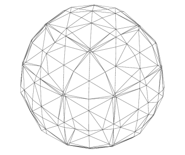
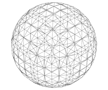
Fig. 1: Approximate interface $\Gamma_{h}$ for a sphere, resulting from a coarse tetrahedral triangulation (left) and after one refinement (right).

Let $\mathcal{F}_{h}$ be the set of all triangular segments $T$, then $\Gamma_{h}$ can be decomposed as

$$\Gamma_{h}=\bigcup\limits_{T\in\mathcal{F}_{h}}T.$$ (7)

Note that the triangulation $\mathcal{F}_{h}$ is not necessarily regular, i.e. elements from $T$ may have very small internal angles and the size of neighboring triangles can vary strongly, cf. Figure 1. In applications with level set functions (that represent $\Gamma$ implicitly), the approximation $\Gamma_{h}$ can be obtained as the zero level of a piecewise linear finite element approximation of the level set function on the tetrahedral triangulation $\mathcal{T}_{h}$.

The surface finite element space is the space of traces on $\Gamma_{h}$ of all piecewise linear continuous functions with respect to the outer triangulation $\mathcal{T}_{h}$. This can be formally defined as follows. We define a subdomain that contains $\Gamma_{h}$:

$$\omega_{h}=\bigcup_{T\in\mathcal{F}_{h}}S_{T},$$ (8)

an a corresponding volume mesh finite element space

$$V_{h}:=\{v_{h}\in C(\omega_{h})\ |\ v_{h}|_{S_{T}}\in P_{1}~{}~{}\forall\ T\in\mathcal{F}_{h}\},$$ (9)

where $P_{1}$ is the space of polynomials of degree one. $V_{h}$ induces the following space on $\Gamma_{h}$:

$$V_{h}^{\Gamma}:=\{\psi_{h}\in H^{1}(\Gamma_{h})\ |\ \exists~{}v_{h}\in V_{h}\ \text{such that }\ \psi_{h}=v_{h}|_{\Gamma_{h}}\}.$$ (10)

When $c=0$, we require that any function $v_{h}$ from $V_{h}^{\Gamma}$ satisfies $\int_{\Gamma_{h}}v_{h}\,\mathrm{d}\mathbf{s}=0$. Given the surface finite element space $V_{h}^{\Gamma}$, the finite element discretization of (5) is as follows: Find $u_{h}\in V_{h}^{\Gamma}$ such that

$$\varepsilon\int_{\Gamma_{h}}\nabla_{\Gamma_{h}}u\cdot\nabla_{\Gamma_{h}}v\,\mathrm{d}\mathbf{s}+\int_{\Gamma_{h}}(\mathbf{w}^{e}\cdot\nabla_{\Gamma_{h}}u)v\,\mathrm{d}\mathbf{s}+\int_{\Gamma_{h}}c\,uv\,\mathrm{d}\mathbf{s}=\int_{\Gamma_{h}}f^{e}v\,\mathrm{d}\mathbf{s}$$ (11)

for all $v_{h}\in V_{h}^{\Gamma}$. Here $\mathbf{w}^{e}$ and $f^{e}$ are the extensions of $\mathbf{w}_{\Gamma}$ and $f$, respectively, along normals to $\Gamma$ (the precise definition is given in the next section). Similar to the plain Galerkin finite element for advection-diffusion equations, the method (11) is unstable unless the mesh is sufficiently fine such that the mesh Peclet number is less than one.

We introduce the following stabilized finite element method based on the standard SUPG approach, cf. [3]: Find $u_{h}\in V_{h}^{\Gamma}$ such that

$$a_{h}(u_{h},v_{h})=f_{h}(v_{h})\quad\forall~{}v_{h}\in V_{h}^{\Gamma},$$ (12)

with

$$a_{h}(u,v):= \varepsilon\int_{\Gamma_{h}}\nabla_{\Gamma_{h}}u\cdot\nabla_{\Gamma_{h}}v\,\mathrm{d}\mathbf{s}+\int_{\Gamma_{h}}c\,uv\mathrm{d}\mathbf{s}$$

$$+\frac{1}{2}\left[\int_{\Gamma_{h}}(\mathbf{w}^{e}\cdot\nabla_{\Gamma_{h}}u)v\,\mathrm{d}\mathbf{s}-\int_{\Gamma_{h}}(\mathbf{w}^{e}\cdot\nabla_{\Gamma_{h}}v)u\,\mathrm{d}\mathbf{s}\right]$$ (13)

$$+\sum_{T\in\mathcal{F}_{h}}\delta_{T}\int_{T}(-\varepsilon\Delta_{\Gamma_{h}}u+\mathbf{w}^{e}\cdot\nabla_{\Gamma_{h}}u+c\,u)\mathbf{w}^{e}\cdot\nabla_{\Gamma_{h}}v\,\mathrm{d}\mathbf{s},$$

$$f_{h}(v):= \int_{\Gamma_{h}}f^{e}v\mathrm{d}\mathbf{s}+\sum_{T\in\mathcal{F}_{h}}\delta_{T}\int_{T}f^{e}(\mathbf{w}^{e}\cdot\nabla_{\Gamma_{h}}v)\,\mathrm{d}\mathbf{s}.$$ (14)

The stabilization parameter $\delta_{T}$ depends on $T\subset S_{T}$. The diameter of the tetrahedron $S_{T}$ is denoted by $h_{S_{T}}$. Let $\displaystyle\mathsf{Pe}_{T}:=\frac{h_{S_{T}}\|\mathbf{w}^{e}\|_{L^{\infty}(T)}}{2\varepsilon}$ be the cell Peclet number. We take

$$\widetilde{\delta_{T}}=\left\{\begin{aligned} &\frac{\delta_{0}h_{S_{T}}}{\|\mathbf{w}^{e}\|_{L^{\infty}(T)}}&&\quad\hbox{ if }\mathsf{Pe}_{T}>1,\\ &\frac{\delta_{1}h^{2}_{S_{T}}}{\varepsilon}&&\quad\hbox{ if }\mathsf{Pe}_{T}\leq 1,\end{aligned}\right.\quad\text{and}\quad\delta_{T}=\min\{\widetilde{\delta_{T}},c^{-1}\},$$ (15)

with some given positive constants $\delta_{0},\delta_{1}\geq 0$.

Since $u_{h}\in V_{h}^{\Gamma}$ is linear on every $T$ we have $\Delta_{\Gamma_{h}}u_{h}=0$ on $T$, and thus $a_{h}(u_{h},v_{h})$ simplifies to

$$a_{h}(u_{h},v_{h})=\varepsilon\int_{\Gamma_{h}}\nabla_{\Gamma_{h}}u_{h}\cdot\nabla_{\Gamma_{h}}v_{h}\,\mathrm{d}\mathbf{s}+\frac{1}{2}\left[\int_{\Gamma_{h}}(\mathbf{w}^{e}\cdot\nabla_{\Gamma_{h}}u_{h})v_{h}-(\mathbf{w}^{e}\cdot\nabla_{\Gamma_{h}}v_{h})u_{h}\,\mathrm{d}\mathbf{s}\right]\\ +\int_{\Gamma_{h}}c\,u_{h}(v_{h}+\delta(\mathbf{x})\mathbf{w}^{e}\cdot\nabla_{\Gamma_{h}}v_{h})\,\mathrm{d}\mathbf{s}+\int_{\Gamma_{h}}\delta(\mathbf{x})(\mathbf{w}^{e}\cdot\nabla_{\Gamma_{h}}u_{h})(\mathbf{w}^{e}\cdot\nabla_{\Gamma_{h}}v_{h})\,\mathrm{d}\mathbf{s},$$ (16)

where $\delta(\mathbf{x})=\delta_{T}$ for $\mathbf{x}\in T$.

3 Error analysis

The analysis in this section is organized as follows. First we collect some definitions and useful results in section 3.1. In section 3.2, we derive a coercivity result. In section 3.3, we present interpolation error bounds. In sections 3.4 and 3.5, continuity and consistency results are derived. Combining these analysis we obtain the finite element error bound given in section 3.6. In the error analysis we use the following mesh-dependent norm:

$$\|u\|_{\ast}:=\left(\varepsilon\int_{\Gamma_{h}}|\nabla_{\Gamma_{h}}u|^{2}\,\mathrm{d}\mathbf{s}+\int_{\Gamma_{h}}\delta(\mathbf{x})|\mathbf{w}^{e}\cdot\nabla_{\Gamma_{h}}u|^{2}\,\mathrm{d}\mathbf{s}+\int_{\Gamma_{h}}c\,|u|^{2}\,\mathrm{d}\mathbf{s}\right)^{\frac{1}{2}}.$$ (17)

Here and in the remainder $|\cdot|$ denotes the Euclidean norm for vectors and the corresponding spectral norm for matrices.

3.1 Preliminaries

For the hypersurface $\Gamma$, we define its $h$-neighborhood:

$$U_{h}:=\{\mathbf{x}\in\mathbb{R}^{3}\ |\ \mathrm{dist}(\mathbf{x},\Gamma)<c_{0}h\},$$ (18)

and assume that $c_{0}$ is sufficiently large such that $\omega_{h}\subset U_{h}$ and $h$ sufficiently small such that

$$5c_{0}h<\left(\mathrm{max}_{i=1,2}\|\kappa_{i}\|_{L^{\infty}(\Gamma)}\right)^{-1}$$ (19)

holds, with $\kappa_{i}$ being the principal curvatures of $\Gamma$. Here and in what follows $h$ denotes the maximum diameter for tetrahedra of outer triangulation: $h=\max\limits_{S\in\omega_{h}}\text{diam}(S)$.

Let $d:U_{h}\rightarrow\mathbb{R}$ be the signed distance function, $|d(\mathbf{x})|=\mathrm{dist}(\mathbf{x},\Gamma)$ for all $\mathbf{x}\in U_{h}$. Thus $\Gamma$ is the zero level set of $d$. We assume $d<0$ in the interior of $\Gamma$ and $d>0$ in the exterior and define $\mathbf{n}(\mathbf{x}):=\nabla d(\mathbf{x})$ for all $\mathbf{x}\in U_{h}$. Hence, $\mathbf{n}=\mathbf{n}_{\Gamma}$ on $\Gamma$ and $|\mathbf{n}(\mathbf{x})|=1$ for all $\mathbf{x}\in U_{h}$. The Hessian of $d$ is denoted by

$$\mathbf{H}(\mathbf{x}):=\nabla^{2}d(\mathbf{x})\in\mathbb{R}^{3\times 3},\quad\mathbf{x}\in U_{h}.$$ (20)

The eigenvalues of $\mathbf{H}(\mathbf{x})$ are denoted by $\kappa_{1}(\mathbf{x})$, $\kappa_{2}(\mathbf{x})$, and $0$. For $\mathbf{x}\in\Gamma$ the eigenvalues $\kappa_{i},i=1,2,$ are the principal curvatures.

For each $\mathbf{x}\in U_{h}$, define the projection $\mathbf{p}:U_{h}\rightarrow\Gamma$ by

$$\mathbf{p}(\mathbf{x})=\mathbf{x}-d(\mathbf{x})\mathbf{n}(\mathbf{x}).$$ (21)

Due to the assumption (19), the decomposition $\mathbf{x}=\mathbf{p}(\mathbf{x})+d(\mathbf{x})\mathbf{n}(\mathbf{x})$ is unique. We will need the orthogonal projector

$$\mathbf{P}(\mathbf{x}):=\mathbf{I}-\mathbf{n}(\mathbf{x})\mathbf{n}(\mathbf{x})^{T},\quad\hbox{for }\mathbf{x}\in U_{h}.$$

Note that $\mathbf{n}(\mathbf{x})=\mathbf{n}(\mathbf{p}(\mathbf{x}))$ and $\mathbf{P}(\mathbf{x})=\mathbf{P}(\mathbf{p}(\mathbf{x}))$ for $\mathbf{x}\in U_{h}$ holds. The tangential derivative can be written as $\nabla_{\Gamma}g(\mathbf{x})=\mathbf{P}\nabla g(\mathbf{x})$ for $\mathbf{x}\in\Gamma$. One can verify that for this projection and for the Hessian $\mathbf{H}$ the relation $\mathbf{H}\mathbf{P}=\mathbf{P}\mathbf{H}=\mathbf{H}$ holds. Similarly, define

$$\mathbf{P}_{h}(\mathbf{x}):=\mathbf{I}-\mathbf{n}_{\Gamma_{h}}(\mathbf{x})\mathbf{n}_{\Gamma_{h}}(\mathbf{x})^{T},\quad\hbox{for }\mathbf{x}\in\Gamma_{h},~{}\mathbf{x}\hbox{ is not on an edge},$$ (22)

where $\mathbf{n}_{\Gamma_{h}}$ is the unit (outward pointing) normal at $\mathbf{x}\in\Gamma_{h}$ (not on an edge). The tangential derivative along $\Gamma_{h}$ is given by $\nabla_{\Gamma_{h}}g(\mathbf{x})=\mathbf{P}_{h}(\mathbf{x})\nabla g(\mathbf{x})$ (not on an edge).

Assumption 3.1.

In this paper, we assume that for all $T\in\mathcal{F}_{h}$:

$$\mathrm{ess\ sup}_{\mathbf{x}\in T}|d(\mathbf{x})|\leq c_{1}h_{S_{T}}^{2},$$ (23)

$$\mathrm{ess\ sup}_{\mathbf{x}\in T}|\mathbf{n}(\mathbf{x})-\mathbf{n}_{\Gamma_{h}}(\mathbf{x})|\leq c_{2}h_{S_{T}},$$ (24)

where $h_{S_{T}}$ denotes the diameter of the tetrahedron $S_{T}$ that contains $T$, i.e., $T=S_{T}\cap\Gamma_{h}$ and constants $c_{1}$, $c_{2}$ are independent of $h$, $T$.

The assumptions (23) and (24) describe how accurate the piecewise planar approximation $\Gamma_{h}$ of $\Gamma$ is. If $\Gamma_{h}$ is constructed as the zero level of a piecewise linear interpolation of a level set function that characterizes $\Gamma$ (as in Fig. 1) then these assumptions are fulfilled, cf. Sect. 7.3 in [1].

In the remainder, $A\lesssim B$ means $A\leq\tilde{c}B$ for some positive constant $\tilde{c}$ independent of $h$ and of the problem parameters $\varepsilon$ and $c$. $A\simeq B$ means that both $A\lesssim B$ and $B\lesssim A$.

For $\mathbf{x}\in\Gamma_{h}$, define

$$\mu_{h}(\mathbf{x})=(1-d(\mathbf{x})\kappa_{1}(\mathbf{x}))(1-d(\mathbf{x})\kappa_{2}(\mathbf{x}))\mathbf{n}^{T}(\mathbf{x})\mathbf{n}_{h}(\mathbf{x}).$$

The surface measures $\mathrm{d}\mathbf{s}$ and $\mathrm{d}\mathbf{s}_{h}$ on $\Gamma$ and $\Gamma_{h}$, respectively, are related by

$$\mu_{h}(\mathbf{x})\mathrm{d}\mathbf{s}_{h}(\mathbf{x})=\mathrm{d}\mathbf{s}(\mathbf{p}(\mathbf{x})),\quad\mathbf{x}\in\Gamma_{h}.$$ (25)

The assumptions (23) and (24) imply that

$$\mathrm{ess\ sup}_{\mathbf{x}\in\Gamma_{h}}(1-\mu_{h})\lesssim h^{2},$$ (26)

cf. (3.37) in [8]. The solution of (4) is defined on $\Gamma$, while its finite element approximation $u_{h}\in V_{h}^{\Gamma}$ is defined on $\Gamma_{h}$. We need a suitable extension of a function from $\Gamma$ to its neighborhood. For a function $v$ on $\Gamma$ we define

$$v^{e}(\mathbf{x}):=v(\mathbf{p}(\mathbf{x}))\quad\hbox{for all }\mathbf{x}\in U_{h}.$$ (27)

The following formula for this lifting function are known (cf. section 2.3 in [13]):

$$\nabla u^{e}(\mathbf{x}) =(\mathbf{I}-d(\mathbf{x})\mathbf{H})\nabla_{\Gamma}u(\mathbf{p}(\mathbf{x}))\quad\hbox{ a.e. on }U_{h},$$ (28)

$$\nabla_{\Gamma_{h}}u^{e}(\mathbf{x}) =\mathbf{P}_{h}(\mathbf{x})(\mathbf{I}-d(\mathbf{x})\mathbf{H})\nabla_{\Gamma}u(\mathbf{p}(\mathbf{x}))\quad\hbox{ a.e. on }\Gamma_{h},$$ (29)

with $\mathbf{H}=\mathbf{H}(\mathbf{x})$. By direct computation one derives the relation

$$\nabla^{2}u^{e}(\mathbf{x})=(\mathbf{P}-d(\mathbf{x})\mathbf{H})\nabla^{2}_{\Gamma}u(\mathbf{p}(\mathbf{x}))(\mathbf{P}-d(\mathbf{x})\mathbf{H})-(n^{T}\nabla_{\Gamma}u(\mathbf{p}(\mathbf{x}))\mathbf{H}\\ -(\mathbf{H}\nabla_{\Gamma}u(\mathbf{p}(\mathbf{x})))\mathbf{n}^{T}-\mathbf{n}(\mathbf{H}\nabla_{\Gamma}u(\mathbf{p}(\mathbf{x})))^{T}-d\nabla_{\Gamma}\mathbf{H}:\nabla_{\Gamma}u(\mathbf{p}(\mathbf{x})).$$ (30)

For sufficiently smooth $u$ and $|\mu|\leq 2$, using this relation one obtains the estimate

$$|D^{\mu}u^{e}(\mathbf{x})|\lesssim\left(\sum_{|\mu|=2}|D_{\Gamma}^{\mu}u(\mathbf{p}(\mathbf{x}))|+|\nabla_{\Gamma}u(\mathbf{p}(\mathbf{x}))|\right)\quad\hbox{a.e. on }U_{h},$$ (31)

(cf. Lemma 3 in [4]). This further leads to (cf. Lemma 3.2 in [8]):

$$\|D^{\mu}u^{e}\|_{L^{2}(U_{h})}\lesssim\sqrt{h}\|u\|_{H^{2}(\Gamma)},\quad|\mu|\leq 2.$$ (32)

The next lemma is needed for the analysis in the following section.

Lemma 1.

The following holds:

$$\|\mathrm{div}_{\Gamma_{h}}\mathbf{w}^{e}\|_{L^{\infty}(\Gamma_{h})}\lesssim h\|\nabla_{\Gamma}\mathbf{w}\|_{L^{\infty}(\Gamma)}.$$

Proof.

We use the following representation for the tangential divergence:

$$\operatorname{div}_{\Gamma}\mathbf{w}(\mathbf{x})=\operatorname{tr}(\nabla_{\Gamma}\mathbf{w}(\mathbf{x}))=\operatorname{tr}(\mathbf{P}\nabla\mathbf{w}(\mathbf{x})).$$ (33)

Take $\mathbf{x}\in\Gamma_{h}$, not lying on an edge. Using (28) we obtain

$$\mathrm{div}_{\Gamma_{h}}\mathbf{w}^{e}(\mathbf{x})$$

$$=\operatorname{tr}(\mathbf{P}_{h}\nabla\mathbf{w}^{e}(\mathbf{x}))=\operatorname{tr}\left(\mathbf{P}_{h}(\mathbf{I}-d(\mathbf{x})\mathbf{H})\nabla_{\Gamma}\mathbf{w}(\mathbf{p}(\mathbf{x}))\right)$$

$$=\operatorname{tr}\left(\mathbf{P}\nabla_{\Gamma}\mathbf{w}(\mathbf{p}(\mathbf{x}))\right)+\operatorname{tr}\left((\mathbf{P}_{h}-\mathbf{P})\nabla_{\Gamma}\mathbf{w}(\mathbf{p}(\mathbf{x}))\right)-d(\mathbf{x})\operatorname{tr}\left(\mathbf{P}_{h}\mathbf{H}\nabla_{\Gamma}\mathbf{w}(\mathbf{p}(\mathbf{x}))\right).$$

The first term vanishes due to $\operatorname{tr}\left(\mathbf{P}\nabla_{\Gamma}\mathbf{w}(\mathbf{p}(\mathbf{x}))\right)=\operatorname{div}_{\Gamma}\mathbf{w}(\mathbf{p}(\mathbf{x}))=0$. The second and the third term can be bounded using (23), (24):

$$|\mathbf{P}_{h}-\mathbf{P}|\lesssim h,\quad|d(\mathbf{x})\mathbf{P}_{h}\mathbf{H}|\lesssim h^{2}.$$

This proves the lemma. ∎

3.2 Coercivity analysis

In the next lemma we present a coercivity result. We use the norm introduced in (17).

Lemma 2.

The following holds:

$$a_{h}(v_{h},v_{h})\geq\frac{1}{2}\|v_{h}\|_{\ast}^{2}\quad\text{for all}~{}~{}v_{h}\in V_{h}^{\Gamma}.$$ (34)

Proof.

For any $v_{h}\in V_{h}^{\Gamma}$, we have

$$a_{h}(v_{h},v_{h})=\|v_{h}\|_{\ast}^{2}+\int_{\Gamma_{h}}c\,\delta(\mathbf{x})v_{h}(\mathbf{w}^{e}\cdot\nabla_{\Gamma_{h}}v_{h})\,\mathrm{d}\mathbf{s}.$$ (35)

The choice of $\delta_{T}$, cf. (15), implies $c\,\delta(\mathbf{x})\leq 1$. Hence the last term in (35) can be estimated as follows:

$$|\int_{\Gamma_{h}}c\,\delta(\mathbf{x})v_{h}(\mathbf{w}^{e}\cdot\nabla_{\Gamma_{h}}v_{h})\,\mathrm{d}\mathbf{s}|$$

$$\leq\frac{1}{2}\int_{\Gamma_{h}}c\,v_{h}^{2}\,\mathrm{d}\mathbf{s}+\frac{1}{2}\int_{\Gamma_{h}}c\,\delta(\mathbf{x})^{2}(\mathbf{w}^{e}\cdot\nabla_{\Gamma_{h}}v_{h})^{2}\,\mathrm{d}\mathbf{s}\leq\frac{1}{2}\|v_{h}\|_{\ast}^{2}.$$

This yields (34). ∎

As a consequence of this result, we obtain the well-posedness of the discrete problem (12).

3.3 Interpolation error bounds

Let $I_{h}:C(\bar{\omega}_{h})\rightarrow V_{h}$ be the nodal interpolation operator. For any $u\in H^{2}(\Gamma)$ the surface finite element function $(I_{h}u^{e})|_{\Gamma_{h}}\in V_{h}^{\Gamma}$ is an interpolant of $u^{e}$ in $V_{h}^{\Gamma}$.

For any $u\in H^{2}(\Gamma)$ the following estimates hold [8]:

$$\|u^{e}-(I_{h}u^{e})|_{\Gamma_{h}}\|_{L^{2}(\Gamma_{h})} \lesssim h^{2}\|u\|_{H^{2}(\Gamma)},$$ (36)

$$\|\nabla_{\Gamma_{h}}u^{e}-\nabla_{\Gamma_{h}}(I_{h}u^{e})|_{\Gamma_{h}}\|_{L^{2}(\Gamma_{h})} \lesssim h\|u\|_{H^{2}(\Gamma)}.$$ (37)

Using these results we easily obtain an interpolation error estimate in the $\|\cdot\|_{\ast}$- norm:

Lemma 3.

For any $u\in H^{2}(\Gamma)$ the following holds:

$$\|u^{e}-(I_{h}u^{e})|_{\Gamma_{h}}\|_{\ast}\lesssim h(\varepsilon^{1/2}+h^{1/2}+c^{\frac{1}{2}}h)\|u\|_{H^{2}(\Gamma)}.$$ (38)

Proof.

Define $\varphi:=u^{e}-(I_{h}u^{e})|_{\Gamma_{h}}\in H^{1}(\Gamma_{h})$. Using the definition (15) of $\delta(\mathbf{x})$, we get

$$\begin{split}\int_{\Gamma_{h}}\delta(\mathbf{x})|\mathbf{w}^{e}\cdot\nabla_{\Gamma_{h}}\varphi|^{2}\mathrm{d}\mathbf{s}&=\sum_{T\in\mathcal{F}_{h}}\int_{T}\delta_{T}|\mathbf{w}^{e}\cdot\nabla_{\Gamma_{h}}\varphi|^{2}\,\mathrm{d}\mathbf{s}\\ &\lesssim h\|\nabla_{\Gamma_{h}}\varphi\|_{L^{2}(\Gamma_{h})}^{2}\lesssim h^{3}\|u\|_{H^{2}(\Gamma)}^{2}.\end{split}$$ (39)

The remaining two terms in $\|u^{e}-(I_{h}u^{e})\|_{\ast}$ are estimated in a straightforward way using (36) and (37). This and (39) imply the inequality (38). ∎

The next lemma estimates the interpolation error on the edges of the surface triangulation. In the remainder, $\mathcal{E}_{h}$ denotes the set of all edges in the interface triangulation $\mathcal{F}_{h}$.

Lemma 4.

For all $u\in H^{2}(\Gamma)$ the following holds:

$$\left(\sum_{E\in\mathcal{E}_{h}}\int_{E}(u^{e}-I_{h}u^{e})|_{\Gamma_{h}}^{2}\,\mathrm{d}\mathbf{s}\right)^{1/2}\lesssim h^{3/2}\|u\|_{H^{2}(\Gamma)}.$$ (40)

Proof.

Define $\phi:=u^{e}-I_{h}u^{e}\in H^{1}(\omega_{h})$. Take $E\in\mathcal{E}_{h}$ and let $T\in\mathcal{F}_{h}$ be a corresponding planar segment of which $E$ is an edge. Let $W$ be a side of the tetrahedron $S_{T}$ such that $E\subset W$. From Lemma 3 in [14] we have

$$\|\phi\|_{L^{2}(E)}^{2}\lesssim h^{-1}\|\phi\|_{L^{2}(W)}^{2}+h\|\phi\|_{H^{1}(W)}^{2}.$$

From the standard trace inequality

$$\|w\|_{L^{2}(\partial S_{T})}^{2}\lesssim h^{-1}\|w\|_{L^{2}(S_{T})}^{2}+h\|w\|_{H^{1}(S_{T})}^{2}\quad\text{for all}~{}~{}w\in H^{1}(S_{T}),$$

applied to $\phi$ and $\partial_{x_{i}}\phi$, $i=1,2,3$, we obtain

$$h^{-1}\|\phi\|_{L^{2}(W)}^{2} \lesssim h^{-2}\|\phi\|_{L^{2}(S_{T})}^{2}+\|\phi\|_{H^{1}(S_{T})}^{2},$$

$$h\|\phi\|_{H^{1}(W)}^{2} \lesssim\|\phi\|_{H^{1}(S_{T})}^{2}+h^{2}\|u^{e}\|_{H^{2}(S_{T})}^{2}.$$

From standard error bounds for the nodal interpolation operator $I_{h}$ we get

$$\|\phi\|_{L^{2}(E)}^{2}\lesssim h^{-2}\|\phi\|_{L^{2}(S_{T})}^{2}+\|\phi\|_{H^{1}(S_{T})}^{2}+h^{2}\|u^{e}\|_{H^{2}(S_{T})}^{2}\lesssim h^{2}\|u^{e}\|_{H^{2}(S_{T})}^{2}.$$

Summing over $E\in\mathcal{E}_{h}$ and using $\|u^{e}\|_{H^{2}(\omega_{h})}\lesssim h^{\frac{1}{2}}\|u\|_{H^{2}(\Gamma)}$, cf. (32), results in

$$\sum_{E\in\mathcal{E}_{h}}\|\phi\|_{L^{2}(E)}^{2}\lesssim h^{2}\|u^{e}\|_{H^{2}(\omega_{h})}^{2}\lesssim h^{3}\|u\|_{H^{2}(\Gamma)}^{2},$$

which completes the proof. ∎

3.4 Continuity estimates

In this section we derive a continuity estimate for the bilinear form $a_{h}(\cdot,\cdot)$. If one applies partial integration to the integrals that occur in $a_{h}(\cdot,\cdot)$ then jumps across the edges $E\in\mathcal{E}_{h}$ occur. We start with a lemma that yields bounds for such jump terms. Related to these jump terms we introduce the following notation. For each $T\in\mathcal{F}_{h}$, denote by ${\mathbf{m}_{h}}|_{E}$ the outer normal to an edge $E$ in the plane which contains element $T$. Let $[\mathbf{m}_{h}]|_{E}=\mathbf{m}_{h}^{+}+\mathbf{m}_{h}^{-}$ be the jump of the outer normals to the edge in two neighboring elements, c.f. Figure 2.

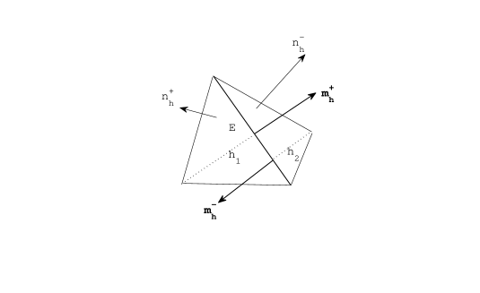
Fig. 2:

Lemma 5.

The following holds:

$$|\mathbf{P}(\mathbf{x})[\mathbf{m}_{h}](\mathbf{x})|\lesssim h^{2}\qquad a.e.\ \mathbf{x}\in E.$$ (41)

Proof.

Let $E$ be the common side of two elements $T_{1}$ and $T_{2}$ in $\mathcal{F}_{h}$, and $\mathbf{n}_{h}^{+}$, $\mathbf{n}_{h}^{-}$, $\mathbf{m}_{h}^{+}$ and $\mathbf{m}_{h}^{-}$ are the unit normals as illustrated in Figure 2. Denote by $\mathbf{s}_{h}$ the unit (constant) vector along the common side $E$, which can be represented as $\mathbf{s}_{h}=\mathbf{n}_{h}^{+}\times\mathbf{m}_{h}^{+}=\mathbf{m}_{h}^{-}\times\mathbf{n}_{h}^{-}$. The jump across $E$ is given by

$$[\mathbf{m}_{h}]=\mathbf{s}_{h}\times(\mathbf{n}_{h}^{+}-\mathbf{n}_{h}^{-}).$$

For each $\mathbf{x}\in E$ and $\mathbf{p}(\mathbf{x})\in\Gamma$, let $\mathbf{n}=\mathbf{n}(\mathbf{p}(\mathbf{x}))$ be the unit normal to $\Gamma$ at $\mathbf{p}(\mathbf{x})$ and $\mathbf{P}=\mathbf{P}(\mathbf{x})=\mathbf{I}-\mathbf{n}\mathbf{n}^{T}$ the corresponding orthogonal projection. Using (24), we get

$$|\mathbf{n}_{h}^{-}-\mathbf{n}_{h}^{+}|\leq|\mathbf{n}_{h}^{+}-\mathbf{n}|+|\mathbf{n}_{h}^{-}-\mathbf{n}|\lesssim h_{S_{T_{1}}}+h_{S_{T_{2}}}\lesssim h.$$

Since $|\mathbf{n}_{h}^{-}|=|\mathbf{n}_{h}^{+}|=|\mathbf{n}|=1$, the above estimate implies

$$\mathbf{n}_{h}^{+}-\mathbf{n}_{h}^{-}=ch^{2}\mathbf{n}+\mathbf{e}_{1},\quad\mathbf{e}_{1}\perp\mathbf{n},\quad|\mathbf{e}_{1}|\lesssim h.$$

We also have

$$\mathbf{s}_{h}=\mathbf{n}_{h}^{+}\times\mathbf{m}_{h}^{+}=(\mathbf{n}+(\mathbf{n}_{h}^{+}-\mathbf{n}))\times\mathbf{m}_{h}^{+}=\mathbf{n}\times\mathbf{m}_{h}^{+}+\mathbf{e}_{2},\quad|\mathbf{e}_{2}|\lesssim h.$$

We use the decomposition

$$\mathbf{P}[\mathbf{m}_{h}]=\mathbf{P}\left[(\mathbf{n}\times\mathbf{m}_{h}^{+}+\mathbf{e}_{2})\times\left(ch^{2}\mathbf{n}+\mathbf{e}_{1}\right)\right].$$

Since $\mathbf{e}_{1}\perp\mathbf{n}$ we have $(\mathbf{n}\times\mathbf{m}_{h}^{+})\times\mathbf{e}_{1}\parallel\mathbf{n}$ and thus $\mathbf{P}\big{(}(\mathbf{n}\times\mathbf{m}_{h}^{+})\times\mathbf{e}_{1}\big{)}=0$. Therefore, we get

$$|\mathbf{P}[\mathbf{m}_{h}]|\lesssim h^{2}+|\mathbf{e}_{1}|\ |\mathbf{e}_{2}|\lesssim h^{2},$$ (42)

i.e., the result (41) holds. ∎

In the analysis below, we need an inequality of the form $\|v_{h}\|_{L^{2}(\Gamma_{h})}\lesssim\|v_{h}\|_{\ast}$ for all $v_{h}\in V_{h}^{\Gamma}$. This result can be obtained as follows. First we consider the case $c=0$. Then the functions $v_{h}\in V_{h}^{\Gamma}$ satisfy $\int_{\Gamma_{h}}v_{h}\,\mathrm{d}\mathbf{s}=0$. We assume that in $V_{h}^{\Gamma}$ a discrete analogon of the Friedrich’s inequality (6) holds uniformly with respect to $h$, i.e., there exists a constant $C_{F}$ independent of $h$ such that

$$\|v_{h}\|_{L^{2}(\Gamma_{h})}^{2}\leq C_{F}\|\nabla_{\Gamma_{h}}v_{h}\|_{L^{2}(\Gamma_{h})}^{2}\quad\text{for all}~{}~{}v_{h}\in V_{h}^{\Gamma}.$$ (43)

Now we reduce the parameter domain $\varepsilon\in(0,1],~{}c>0$ as follows. For a given generic constant $c_{0}$ with $0<c_{0}<1$, in the remainder we restrict to the parameter set

$$\varepsilon\in(0,1],~{}~{}c\in\{0\}\cup[c_{0}\varepsilon,\infty).$$ (44)

For $c>0$ we then have

$$c_{0}\|v_{h}\|_{L^{2}(\Gamma_{h})}^{2} \leq\frac{2c_{0}}{c_{0}+1}\frac{1}{c}\|c^{\frac{1}{2}}v_{h}\|_{L^{2}(\Gamma_{h})}^{2}\leq\frac{2}{c/c_{0}+c}\|v_{h}\|_{\ast}^{2}\leq\frac{2}{\varepsilon+c}\|v_{h}\|_{\ast}^{2},$$

and combing this with the result in (43) for the case $c=0$ we get

$$\|v_{h}\|_{L^{2}(\Gamma_{h})}\lesssim\frac{1}{\sqrt{\varepsilon+c}}\|v_{h}\|_{\ast}\quad\text{for all}~{}~{}v_{h}\in V_{h}^{\Gamma}$$ (45)

and arbitrary $\varepsilon\in(0,1],~{}c\in\{0\}\cup[c_{0}\varepsilon,\infty)$.

In the proof of Theorem 8 below we need a bound for $\|v_{h}\|_{L^{2}(\mathcal{E}_{h})}$ in terms of $\|v_{h}\|_{\ast}$. Such a result is derived with the help of the following lemma.

Lemma 6.

Assume the outer tetrahedra mesh size satisfies $h\leq h_{0}$, with some sufficiently small $h_{0}\simeq 1$, depending only on the constant $c_{2}$ from (24). The following holds:

$$\sum_{E\in\mathcal{E}_{h}}\int_{E}v_{h}^{2}\,\mathrm{d}\mathbf{s}\lesssim h^{-1}\|v_{h}\|^{2}_{L^{2}(\Gamma_{h})}+h\|\nabla_{\Gamma_{h}}v_{h}\|^{2}_{L^{2}(\Gamma_{h})}\quad\text{for all}~{}~{}v_{h}\in V_{h}^{\Gamma}$$ (46)

Proof.

Let $E\in\mathcal{E}_{h}$ be an edge of a triangle $T\in\mathcal{F}_{h}$ and $S_{T}\in\mathcal{T}_{h}$ is the corresponding tetrahedron of the outer triangulation. Consider the patch $\widetilde{\omega}(S_{T})$ of all $S\in\mathcal{T}_{h}$ touching $S_{T}$. Denote $\omega(S_{T})=\widetilde{\omega}(S_{T})\cap\Gamma_{h}$. Let $v_{h}$ be an arbitrary fixed function from $V_{h}^{\Gamma}$. We shall prove the bound

$$\int_{E}v_{h}^{2}\,\mathrm{d}\mathbf{s}\lesssim h^{-1}\|v_{h}\|^{2}_{L^{2}(\omega(S_{T}))}+h\|\nabla_{\Gamma_{h}}v_{h}\|^{2}_{L^{2}(\omega(S_{T}))}.$$ (47)

Then summing over all $E\in\mathcal{E}_{h}$ and using that $\omega(S_{T})$ consists of a uniformly bounded number of tetrahedra (due to the regularity of the outer mesh), we obtain (46).

Let $\mathbb{P}$ be a plane containing $T$. We can define for sufficiently small $h$ an injective mapping $\phi:\omega(S_{T})\to\mathbb{P}$ such that $|\nabla\phi|\lesssim 1$ and $|\nabla(\phi^{-1})|\lesssim 1$. For example, $\phi$ can be build by the orthogonal projection on $\mathbb{P}$. Then $|\nabla\phi|\lesssim 1$ and $|\nabla(\phi^{-1})(\mathbf{x})|\lesssim(\sin\alpha)^{-1}$, where $\alpha$ is the angle between $\mathbb{P}$ and $\mathbf{n}_{h}(\phi^{-1}(\mathbf{x}))$. Due to assumption (24) we have $1\lesssim\sin\alpha$ for sufficiently small $h$. If $\phi$ is the orthogonal projection on $\mathbb{P}$, then $\phi(E)=E$. Thus we get

$$\left\{\begin{split}\int_{E}v_{h}^{2}\mathrm{d}\mathbf{s}&=\int_{\phi(E)}(v_{h}\circ\phi^{-1})^{2}\mathrm{d}\mathbf{s},\\ \|v_{h}\|_{L^{2}(\omega(S_{T}))}&\simeq\|v_{h}\circ\phi^{-1}\|_{L^{2}(\phi(\omega(S_{T})))},\\ \|\nabla_{\Gamma_{h}}v_{h}\|_{L^{2}(\omega(S_{T}))}&\simeq\|\nabla_{\mathbb{P}}(v_{h}\circ\phi^{-1})\|_{L^{2}(\phi(\omega(S_{T})))}.\end{split}\right.$$ (48)

Due to the shape regularity of $S\in\widetilde{\omega}(S_{T})$ we have

$$h\lesssim\text{dist}(E,\partial\,\widetilde{\omega}(S_{T}))\leq\text{dist}(E,\partial\,\omega(S_{T})).$$

Hence, from $|\nabla\phi^{-1}|\lesssim 1$ it follows that $h\lesssim\text{dist}(\phi(E),\partial\,\phi(\omega(S_{T})))$. Thus, we may consider a rectangle $Q\subset\phi(\omega(S_{T}))$ such that $E=\phi(E)$ is a side of $Q$ and $|Q|\simeq h|E|$. By the standard trace theorem and scaling argument we get

$$\int_{\phi(E)}(v_{h}\circ\phi^{-1})^{2}\mathrm{d}\mathbf{s}\lesssim h^{-1}\|v_{h}\circ\phi^{-1}\|^{2}_{L^{2}(Q)}+h\|\nabla_{\mathbb{P}}(v_{h}\circ\phi^{-1})\|^{2}_{L^{2}(Q)}.$$

This together with (48) and $Q\subset\phi(\omega(S_{T}))$ implies (47). ∎

An immediate consequence of the lemma and (45) is the following corollary.

Corollary 7.

The following estimate holds:

$$h\sum_{E\in\mathcal{E}_{h}}\int_{E}v_{h}^{2}\,\mathrm{d}\mathbf{s}\lesssim\big{(}\frac{1}{\varepsilon+c}+\frac{h^{2}}{\varepsilon}\big{)}\|v_{h}\|_{\ast}^{2}\quad\text{for all}~{}~{}v_{h}\in V_{h}^{\Gamma}.$$ (49)

We are now in position to prove a continuity result for the surface finite element bilinear form.

Lemma 8.

For any $u\in H^{2}(\Gamma)$ and $v_{h}\in V_{h}^{\Gamma}$, we have

$$|a_{h}(u^{e}-(I_{h}u^{e})|_{\Gamma_{h}},v_{h})|\lesssim\left(\varepsilon^{1/2}+h^{1/2}+c^{\frac{1}{2}}h+\frac{h^{2}}{\sqrt{\varepsilon+c}}+\frac{h^{3}}{\sqrt{\varepsilon}}\right)h\|u\|_{H^{2}(\Gamma)}\|v_{h}\|_{\ast}.$$ (50)

Proof.

Define $\phi=u^{e}-(I_{h}u^{e})|_{{\Gamma_{h}}}$, then

$$\begin{split}a_{h}(\phi,v_{h})&=\varepsilon\int_{\Gamma_{h}}\nabla_{\Gamma_{h}}\phi\cdot\nabla_{\Gamma_{h}}v_{h}\mathrm{d}\mathbf{s}\\ &+\int_{\Gamma_{h}}\frac{1}{2}\big{(}(\mathbf{w}^{e}\cdot\nabla_{\Gamma_{h}}\phi)v_{h}-(\mathbf{w}^{e}\cdot\nabla_{\Gamma_{h}}v_{h})\phi\big{)}+c\,\phi v_{h}\,\mathrm{d}\mathbf{s}\\ &+\sum_{T\in\mathcal{F}_{h}}\delta_{T}\int_{T}\left(-\varepsilon\Delta_{\Gamma_{h}}\phi+\mathbf{w}^{e}\cdot\nabla_{\Gamma_{h}}\phi+c\phi\right)\mathbf{w}^{e}\cdot\nabla_{\Gamma_{h}}v_{h}\,\mathrm{d}\mathbf{s}.\end{split}$$ (51)

We estimate $a_{h}(\phi,v_{h})$ term by term. Due to (36), (37), we get for the first term on the righthand side of (51):

$$\Big{|}\varepsilon\int_{\Gamma_{h}}\nabla_{\Gamma_{h}}\phi\cdot\nabla_{\Gamma_{h}}v_{h}\mathrm{d}\mathbf{s}\Big{|}\lesssim\varepsilon h\|u\|_{H^{2}(\Gamma)}\|\nabla_{\Gamma_{h}}v_{h}\|_{L^{2}(\Gamma_{h})}\leq\varepsilon^{\frac{1}{2}}h\|u\|_{H^{2}(\Gamma)}\|v_{h}\|_{\ast}.$$ (52)

To the second term on the righthand side of (51) we apply integration by parts:

$$\begin{split}&\int_{\Gamma_{h}}\frac{1}{2}\big{(}(\mathbf{w}^{e}\cdot\nabla_{\Gamma_{h}}\phi)v_{h}-(\mathbf{w}^{e}\cdot\nabla_{\Gamma_{h}}v_{h})\phi\big{)}+c\phi v_{h}\,\mathrm{d}\mathbf{s}\\ &=\int_{\Gamma_{h}}c\phi v_{h}\mathrm{d}\mathbf{s}-\int_{\Gamma_{h}}(\mathbf{w}^{e}\cdot\nabla_{\Gamma_{h}}v_{h})\phi\mathrm{d}\mathbf{s}\\ &+\frac{1}{2}\sum_{T\in\mathcal{F}_{h}}\int_{\partial T}(\mathbf{w}^{e}\cdot\mathbf{m}_{h})\phi v_{h}\mathrm{d}\mathbf{s}-\frac{1}{2}\int_{\Gamma_{h}}(\mathrm{div}_{\Gamma_{h}}\mathbf{w}^{e})\phi v_{h}\mathrm{d}\mathbf{s}\\ &=:I_{1}+I_{2}+I_{3}+I_{4}.\end{split}$$ (53)

The term $I_{1}$ can be estimated by

$$|I_{1}|\lesssim c^{\frac{1}{2}}\|\phi\|_{L^{2}(\Gamma_{h})}\|\sqrt{c}v_{h}\|_{L^{2}(\Gamma_{h})}\lesssim h^{2}c^{\frac{1}{2}}\|u\|_{H^{2}(\Gamma)}\|v_{h}\|_{\ast}.$$

To estimate $I_{2}$, we consider the advection-dominated case and the diffusion-dominated case separately. If $\mathsf{Pe}_{T}>1$, we have

$$\int_{T}(\mathbf{w}^{e}\cdot\nabla_{\Gamma_{h}}v_{h})\phi\mathrm{d}\mathbf{s} \lesssim\delta_{T}^{-1/2}\|\phi\|_{L^{2}(T)}\left(\int_{T}\delta_{T}(\mathbf{w}^{e}\cdot\nabla_{\Gamma_{h}}v_{h})^{2}\mathrm{d}\mathbf{s}\right)^{1/2}$$

$$\lesssim{\max(h^{-1/2},c^{1/2})}\|\phi\|_{L^{2}(T)}\left(\int_{T}\delta_{T}(\mathbf{w}^{e}\cdot\nabla_{\Gamma_{h}}v_{h})^{2}\mathrm{d}\mathbf{s}\right)^{1/2},$$

and if $\mathsf{Pe}_{T}\leq 1$:

$$\int_{T}(\mathbf{w}^{e}\cdot\nabla_{\Gamma_{h}}v_{h})\phi\mathrm{d}\mathbf{s} \lesssim\|\mathbf{w}^{e}\|_{L^{\infty}(T)}\|\nabla_{\Gamma_{h}}v_{h}\|_{L^{2}(T)}\|\phi\|_{L^{2}(T)}$$

$$\lesssim\varepsilon^{1/2}h^{-1}\|\varepsilon^{1/2}\nabla_{\Gamma_{h}}v_{h}\|_{L^{2}(T)}\|\phi\|_{L^{2}(T)}.$$

Summing over $T\in\mathcal{F}_{h}$ we obtain

$$|I_{2}|\lesssim(h^{-1/2}+\varepsilon^{1/2}h^{-1})\|\phi\|_{L^{2}(\Gamma_{h})}\|v_{h}\|_{\ast}\lesssim h(c^{1/2}h+h^{1/2}+\varepsilon^{1/2})\|u\|_{H^{2}(\Gamma)}\|v_{h}\|_{\ast}.$$

The term $I_{3}$ is estimated using $\mathbf{P}\mathbf{w}^{e}=\mathbf{w}^{e}$, Lemmas 4, 5, and Corollary 7:

$$|I_{3}| \lesssim\Big{|}\sum_{E\in\mathcal{E}_{h}}\int_{E}(\mathbf{w}^{e}\cdot[\mathbf{m}_{h}])\phi v_{h}\mathrm{d}\mathbf{s}\Big{|}$$ (54)

$$\lesssim\left(\sum_{E\in\mathcal{E}_{h}}\int_{E}|\phi|^{2}\mathrm{d}\mathbf{s}\right)^{1/2}\left(\sum_{E\in\mathcal{E}_{h}}\int_{E}|\mathbf{P}[\mathbf{m}_{h}]|^{2}v_{h}^{2}\,\mathrm{d}\mathbf{s}\right)^{1/2}$$

$$\lesssim h^{3}\|u\|_{H^{2}(\Gamma)}\left(h\sum_{E\in\mathcal{E}_{h}}\int_{E}v_{h}^{2}\,\mathrm{d}\mathbf{s}\right)^{1/2}\lesssim\left(\frac{h^{3}}{\sqrt{\varepsilon+c}}+\frac{h^{4}}{\sqrt{\varepsilon}}\right)\|u\|_{H^{2}(\Gamma)}\|v_{h}\|_{\ast}.$$

The term $I_{4}$ in (53) can be bounded due to Lemma 1, the interpolation bounds and (45):

$$|I_{4}| \leq\frac{1}{2}\|\mathrm{div}_{\Gamma_{h}}\mathbf{w}^{e}\|_{L^{\infty}(\Gamma_{h})}\|\phi\|_{L^{2}(\Gamma_{h})}\|v_{h}\|_{L^{2}(\Gamma_{h})}\lesssim h^{3}\|u\|_{H^{2}(\Gamma)}\|v_{h}\|_{L^{2}(\Gamma_{h})}$$

$$\leq\frac{h^{3}}{\sqrt{\varepsilon+c}}\|u\|_{H^{2}(\Gamma)}\|v_{h}\|_{\ast}.$$

Finally we treat the third term on the righthand side of (51). Using $\delta_{T}\|\mathbf{w}^{e}\|_{L^{\infty}(T)}\lesssim h$, $\delta_{T}\varepsilon\lesssim 1$, $\delta_{T}c\leq 1$ and the interpolation estimates (36) and (37) we obtain:

$$\sum_{T\in\mathcal{F}_{h}}\delta_{T}\int_{T}(-\varepsilon\Delta_{\Gamma_{h}}\phi+\mathbf{w}^{e}\cdot\nabla_{\Gamma_{h}}\phi+c\phi)\mathbf{w}^{e}\cdot\nabla_{\Gamma_{h}}v_{h}\,\mathrm{d}\mathbf{s}$$ (55)

$$\lesssim \left(\sum_{T\in\mathcal{F}_{h}}\delta_{T}\big{(}\varepsilon^{2}\|\Delta_{\Gamma_{h}}u^{e}\|^{2}_{L^{2}(T)}+\|\mathbf{w}^{e}\cdot\nabla_{\Gamma_{h}}\phi\|^{2}_{L^{2}(T)}+c^{2}\|\phi\|^{2}_{L^{2}(T)}\big{)}\right)^{1/2}\|v_{h}\|_{\ast}$$

$$\lesssim ~{}(\varepsilon^{1/2}+h^{1/2}+c^{\frac{1}{2}}h)h\|u\|_{H^{2}(\Gamma)}\|v_{h}\|_{\ast}.$$

Combing the inequalities (52)–(55) proves the result of the lemma. ∎

3.5 Consistency estimate

The consistency error of the finite element method (12) is due to geometric errors resulting from the approximation of $\Gamma$ by $\Gamma_{h}$. To estimate this geometric errors we need a few additional definitions and results, which can be found in, for example, [13]. For $\mathbf{x}\in\Gamma_{h}$ define $\tilde{\mathbf{P}}_{h}(\mathbf{x})=\mathbf{I}-\mathbf{n}_{h}(\mathbf{x})\mathbf{n}(\mathbf{x})^{T}/(\mathbf{n}_{h}(\mathbf{x})\cdot\mathbf{n}(\mathbf{x}))$. One can represent the surface gradient of $u\in H^{1}(\Gamma)$ in terms of $\nabla_{\Gamma_{h}}u^{e}$ as follows

$$\nabla_{\Gamma}u(\mathbf{p}(\mathbf{x}))=(\mathbf{I}-d(\mathbf{x})\mathbf{H}(\mathbf{x}))^{-1}\tilde{\mathbf{P}}_{h}(\mathbf{x})\nabla_{\Gamma_{h}}u^{e}(\mathbf{x})~{}~{}\hbox{ a.e. }\mathbf{x}\in\Gamma_{h}.$$ (56)

Due to (25), we get

$$\int_{\Gamma}\nabla_{\Gamma}u\nabla_{\Gamma}v\,\mathrm{d}\mathbf{s}=\int_{\Gamma_{h}}\mathbf{A}_{h}\nabla_{\Gamma_{h}}u^{e}\nabla_{\Gamma_{h}}v^{e}\,\mathrm{d}\mathbf{s}\quad\hbox{for all }v\in H^{1}(\Gamma),$$ (57)

with $\mathbf{A}_{h}(\mathbf{x})=\mu_{h}(\mathbf{x})\tilde{\mathbf{P}}^{T}_{h}(\mathbf{x})(\mathbf{I}-d(\mathbf{x})\mathbf{H}(\mathbf{x}))^{-2}\tilde{\mathbf{P}}_{h}(\mathbf{x})$. From $\mathbf{w}\cdot\mathbf{n}=0$ on $\Gamma$ and $\mathbf{w}^{e}(\mathbf{x})=\mathbf{w}(\mathbf{p}(\mathbf{x}))$, $\mathbf{n}(\mathbf{x})=\mathbf{n}(\mathbf{p}(\mathbf{x}))$ it follows that $\mathbf{n}(\mathbf{x})\cdot\mathbf{w}^{e}(\mathbf{x})=0$ and thus $\mathbf{w}(\mathbf{p}(\mathbf{x}))=\tilde{\mathbf{P}}_{h}(\mathbf{x})\mathbf{w}^{e}(\mathbf{x})$ holds. Using this, we get the relation

$$\int_{\Gamma}(\mathbf{w}\cdot\nabla_{\Gamma}u)v\,\mathrm{d}\mathbf{s}=\int_{\Gamma_{h}}(\mathbf{B}_{h}\mathbf{w}^{e}\cdot\nabla_{\Gamma_{h}}u^{e})v^{e}\,\mathrm{d}\mathbf{s},$$ (58)

with $\mathbf{B}_{h}=\mu_{h}(\mathbf{x})\tilde{\mathbf{P}}_{h}^{T}(I-d\mathbf{H})^{-1}\tilde{\mathbf{P}}_{h}$. In the proof we use the lifting procedure $\Gamma_{h}\to\Gamma$ given by

$$v_{h}^{l}(\mathbf{p}(\mathbf{x})):=v_{h}(\mathbf{x})\quad\text{for}~{}~{}\mathbf{x}\in\Gamma_{h}.$$ (59)

It is easy to see that $v_{h}^{l}\in H^{1}(\Gamma)$.

The following lemma estimates the consistency error of the finite element method (12).

Lemma 9.

Let $u\in H^{2}(\Gamma)$ be the solution of (5), then we have

$$\sup_{v_{h}\in V_{h}^{\Gamma}}\frac{|f_{h}(v_{h})-a_{h}(u^{e},v_{h})|}{\|v_{h}\|_{\ast}}\lesssim\big{(}h^{\frac{1}{2}}+c^{\frac{1}{2}}h+\frac{h}{\sqrt{c+\varepsilon}}\big{)}\,h(\|u\|_{H^{2}(\Gamma)}+\|f\|_{L^{2}(\Gamma)}).$$ (60)

Proof.

The residual is decomposed as

$$f_{h}(v_{h})-a_{h}(u^{e},v_{h})=f_{h}(v_{h})-f(v_{h}^{l})+a(u,v_{h}^{l})-a_{h}(u^{e},v_{h}).$$ (61)

The following holds:

$$f(v^{l}_{h})= \,\int_{\Gamma}fv_{h}^{l}\,\mathrm{d}\mathbf{s}=\int_{\Gamma_{h}}\mu_{h}f^{e}v_{h}\,\mathrm{d}\mathbf{s},$$

$$a(u,v^{l}_{h})= \,\varepsilon\int_{\Gamma}\nabla_{\Gamma}u\nabla_{\Gamma}v_{h}^{l}\,\mathrm{d}\mathbf{s}+\int_{\Gamma}(\mathbf{w}\cdot\nabla_{\Gamma}u)v_{h}^{l}\mathrm{d}\mathbf{s}+\int_{\Gamma}cuv_{h}^{l}\,\mathrm{d}\mathbf{s}$$

$$= \,\varepsilon\int_{\Gamma}\nabla_{\Gamma}u\nabla_{\Gamma}v_{h}^{l}\,\mathrm{d}\mathbf{s}+\frac{1}{2}\int_{\Gamma}(\mathbf{w}\cdot\nabla_{\Gamma}u)v_{h}^{l}-(\mathbf{w}\cdot\nabla_{\Gamma}v_{h}^{l})u\,\mathrm{d}\mathbf{s}+\int_{\Gamma}cuv_{h}^{l}\,\mathrm{d}\mathbf{s}$$

$$= \,\varepsilon\int_{\Gamma_{h}}\mathbf{A}_{h}\nabla_{\Gamma_{h}}u^{e}\nabla_{\Gamma_{h}}v_{h}\,\mathrm{d}\mathbf{s}+\frac{1}{2}\int_{\Gamma_{h}}(\mathbf{B}_{h}\mathbf{w}^{e}\cdot\nabla_{\Gamma_{h}}u^{e})v_{h}\,\mathrm{d}\mathbf{s}$$

$$\,-\frac{1}{2}\int_{\Gamma_{h}}(\mathbf{B}_{h}\mathbf{w}^{e}\cdot\nabla_{\Gamma_{h}}v_{h})u^{e}\,\mathrm{d}\mathbf{s}+\int_{\Gamma_{h}}\mu_{h}cu^{e}v_{h}\,\mathrm{d}\mathbf{s}.$$

Substituting these relations into (61) and using (13), (14) results in

$$f_{h}(v_{h})-a_{h}(u^{e},v_{h})=\int_{\Gamma_{h}}(1-\mu_{h})f^{e}v_{h}\,\mathrm{d}\mathbf{s}+\varepsilon\int_{\Gamma_{h}}(\mathbf{A}_{h}-\mathbf{P}_{h})\nabla_{\Gamma_{h}}u^{e}\cdot\nabla_{\Gamma_{h}}v_{h}\,\mathrm{d}\mathbf{s}\\ +\frac{1}{2}\int_{\Gamma_{h}}((\mathbf{B}_{h}-\mathbf{P}_{h})\mathbf{w}^{e}\cdot\nabla_{\Gamma_{h}}u^{e})v_{h}\,\mathrm{d}\mathbf{s}-\frac{1}{2}\int_{\Gamma_{h}}((\mathbf{B}_{h}-\mathbf{P}_{h})\mathbf{w}^{e}\cdot\nabla_{\Gamma_{h}}v_{h})u^{e}\,\mathrm{d}\mathbf{s}\\ +\int_{\Gamma_{h}}(\mu_{h}-1)cu^{e}v_{h}\,\mathrm{d}\mathbf{s}+\sum_{T\in\mathcal{F}_{h}}\delta_{T}\int_{T}\big{(}f^{e}+\varepsilon\Delta_{\Gamma_{h}}u^{e}-\mathbf{w}^{e}\cdot\nabla_{\Gamma_{h}}u^{e}-cu^{e}\big{)}\mathbf{w}^{e}\cdot\nabla_{\Gamma_{h}}v_{h}\,\mathrm{d}\mathbf{s}\\ =:I_{1}+I_{2}+I_{3}+I_{4}+I_{5}+\varPi_{1}.$$ (62)

We estimate the $I_{i}$ terms separately. Applying (26) and (45) we get

$$I_{1} \lesssim h^{2}\|f^{e}\|_{L^{2}(\Gamma_{h})}\|v_{h}\|_{L^{2}(\Gamma_{h})}\lesssim\frac{h^{2}}{\sqrt{c+\varepsilon}}\|f\|_{L^{2}(\Gamma)}\|v_{h}\|_{\ast},$$ (63)

$$I_{5} \lesssim h^{2}c^{\frac{1}{2}}\|u^{e}\|_{L^{2}(\Gamma_{h})}\|\sqrt{c}v_{h}\|_{L^{2}(\Gamma_{h})}\lesssim h^{2}c^{\frac{1}{2}}\|u\|_{L^{2}(\Gamma)}\|v_{h}\|_{\ast}.$$ (64)

One can show, cf. (3.43) in [8], the bound

$$|\mathbf{P}_{h}-\mathbf{A}_{h}|=|\mathbf{P}_{h}(\mathbf{I}-\mathbf{A}_{h})|\lesssim h^{2}.$$

Using this we obtain

$$I_{2}\lesssim\varepsilon h^{2}\|\nabla_{\Gamma_{h}}u^{e}\|_{L^{2}(\Gamma_{h})}\|\nabla_{\Gamma_{h}}v_{h}\|_{L^{2}(\Gamma_{h})}\lesssim\varepsilon^{1/2}h^{2}\|u^{e}\|_{H^{2}(\Gamma)}\|v_{h}\|_{\ast}.$$ (65)

Since $(\mathbf{I}-d\mathbf{H})^{-1}=\mathbf{I}+O(h^{2})$, we also estimate

$$|\mathbf{B}_{h}-\mathbf{P}_{h}|\lesssim h^{2}+|\mathbf{A}_{h}-\mathbf{P}_{h}|\lesssim h^{2}.$$

This yields

$$I_{3}\lesssim h^{2}\|\nabla_{\Gamma_{h}}u^{e}\|_{L^{2}(\Gamma_{h})}\|v_{h}\|_{L^{2}(\Gamma_{h})}\lesssim\frac{h^{2}}{\sqrt{c+\varepsilon}}\|u\|_{H^{2}(\Gamma)}\|v_{h}\|_{\ast}.$$ (66)

To estimate $I_{4}$ we use the definition (15) of $\delta_{T}$. If $\displaystyle\mathsf{Pe}_{T}\leq 1$, then $\varepsilon^{-\frac{1}{2}}\|\mathbf{w}^{e}\|_{L^{\infty}(T)}\leq\sqrt{2}\|\mathbf{w}^{e}\|_{L^{\infty}(T)}^{\frac{1}{2}}h_{S_{T}}^{-\frac{1}{2}}$ holds. If $\displaystyle\mathsf{Pe}_{T}>1$, then $\delta_{T}^{-\frac{1}{2}}\leq{\max(c^{\frac{1}{2}},\delta_{0}^{-\frac{1}{2}}\|\mathbf{w}^{e}\|_{L^{\infty}(T)}^{\frac{1}{2}}h_{S_{T}}^{-\frac{1}{2}})}$ holds. Using the assumption that the outer triangulation is quasi-uniform we get $h_{S_{T}}^{-1}\lesssim h^{-1}$. Thus, we obtain

$$\min\{\varepsilon^{-\frac{1}{2}}\|\mathbf{w}^{e}\|_{L^{\infty}(T)},\delta_{T}^{-\frac{1}{2}}\}\lesssim{\max(c^{\frac{1}{2}},h^{-\frac{1}{2}})\lesssim c^{\frac{1}{2}}+h^{-\frac{1}{2}}},$$

and

$$I_{4}\lesssim \max_{x\in\Gamma_{h}}|\mathbf{B}_{h}-\mathbf{P}_{h}|\sum_{T\in\mathcal{F}_{h}}(\varepsilon^{\frac{1}{2}}\|\nabla_{\Gamma_{h}}v_{h}\|_{L^{2}(T)}+\delta_{T}^{\frac{1}{2}}\|\mathbf{w}^{e}_{\Gamma_{h}}\cdot\nabla_{\Gamma_{h}}v_{h}\|_{L^{2}(T)})$$

$$~{}~{}\times\min\{\varepsilon^{-\frac{1}{2}}\|\mathbf{w}^{e}\|_{L^{\infty}(T)},\delta_{T}^{-\frac{1}{2}}\}\|u^{e}\|_{L^{2}(T)}$$

$$\lesssim ~{}{h(c^{\frac{1}{2}}h+h^{\frac{1}{2}})}\|v_{h}\|_{\ast}\|u\|_{L^{2}(\Gamma)}.$$ (67)

Now we estimate $\varPi_{1}$. Using the equation $-\varepsilon\Delta_{\Gamma}u+\mathbf{w}\cdot\nabla_{\Gamma}u+cu=f$ on $\Gamma$ we get

$$\varPi_{1} =\sum_{T\in\mathcal{F}_{h}}\delta_{T}\int_{T}\big{(}f\circ\mathbf{p}+\varepsilon\Delta_{\Gamma_{h}}u^{e}-\mathbf{w}^{e}\cdot\nabla_{\Gamma_{h}}u^{e}-cu^{e}\big{)}\mathbf{w}^{e}\cdot\nabla_{\Gamma_{h}}v_{h}\,\mathrm{d}\mathbf{s}$$

$$=\sum_{T\in\mathcal{F}_{h}}\delta_{T}\int_{T}\big{(}-\varepsilon(\Delta_{\Gamma}u)\circ\mathbf{p}+\varepsilon\Delta_{\Gamma_{h}}u^{e}\big{)}\mathbf{w}^{e}\cdot\nabla_{\Gamma_{h}}v_{h}\,\mathrm{d}\mathbf{s}$$

$$\quad+\sum_{T\in\mathcal{F}_{h}}\delta_{T}\int_{T}\big{(}(\mathbf{w}^{e}\cdot\nabla_{\Gamma}u)\circ\mathbf{p}-\mathbf{w}^{e}\cdot\nabla_{\Gamma_{h}}u^{e}\big{)}\mathbf{w}^{e}\cdot\nabla_{\Gamma_{h}}v_{h}\,\mathrm{d}\mathbf{s}$$

$$\quad+\sum_{T\in\mathcal{F}_{h}}\delta_{T}\int_{T}\big{(}cu\circ\mathbf{p}-cu^{e}\big{)}\mathbf{w}^{e}\cdot\nabla_{\Gamma_{h}}v_{h}\,\mathrm{d}\mathbf{s}$$

$$=:\varPi_{1}^{1}+\varPi_{1}^{2}+\varPi_{1}^{3}.$$ (68)

From $u^{e}=u\circ\mathbf{p}$ it follows that $\varPi_{1}^{3}=0$ holds. For $\varPi_{1}^{2}$ we obtain, using (56) and $|\mu_{h}^{-1}\mathbf{B}_{h}-\mathbf{P}_{h}|\leq|\mu_{h}-1||\mu_{h}|^{-1}|\mathbf{B}_{h}|+|\mathbf{B}_{h}-\mathbf{P}_{h}|\lesssim h^{2}$,

$$\varPi_{1}^{2} =\sum_{T\in\mathcal{F}_{h}}\delta_{T}\int_{T}\big{(}(\mu_{h}^{-1}\mathbf{B}_{h}-\mathbf{P}_{h})\mathbf{w}^{e}\cdot\nabla_{\Gamma_{h}}u^{e}\big{)}\mathbf{w}^{e}\cdot\nabla_{\Gamma_{h}}v_{h}\,\mathrm{d}\mathbf{s}$$

$$\lesssim h^{2}\left(\sum_{T\in\mathcal{F}_{h}}\delta_{T}\|\mathbf{w}^{e}\|_{L^{\infty}}^{2}\|\nabla_{\Gamma_{h}}u^{e}\|_{L^{2}(T)}^{2}\right)^{\frac{1}{2}}\left(\sum_{T\in\mathcal{F}_{h}}\delta_{T}\|\mathbf{w}^{e}\cdot\nabla_{\Gamma_{h}}v_{h}\|_{L^{2}(T)}^{2}\right)^{\frac{1}{2}}$$

$$\lesssim h^{\frac{5}{2}}\|u\|_{H^{2}(\Gamma)}\|v_{h}\|_{\ast}.$$ (69)

Since $\delta_{T}\varepsilon\lesssim h^{2}$, we get

$$\varPi_{2}^{1} \lesssim\left(\sum_{T\in\mathcal{F}_{h}}\varepsilon^{2}\delta_{T}\|(\Delta_{\Gamma}u)\circ\mathbf{p}-\Delta_{\Gamma_{h}}u^{e}\|_{L^{2}(T)}^{2}\right)^{\frac{1}{2}}\left(\sum_{T\in\mathcal{F}_{h}}\delta_{T}\|\mathbf{w}^{e}\cdot\nabla_{\Gamma_{h}}v_{h}\|_{L^{2}(T)}^{2}\right)^{\frac{1}{2}}$$

$$\lesssim h\varepsilon^{\frac{1}{2}}\left(\sum_{T\in\mathcal{F}_{h}}\|(\Delta_{\Gamma}u)\circ\mathbf{p}-\Delta_{\Gamma_{h}}u^{e}\|_{L^{2}(T)}^{2}\right)^{\frac{1}{2}}\|v_{h}\|_{\ast}.$$ (70)

We finally consider the term between brackets in (3.5). Using the identity $\operatorname{div}_{\Gamma}\mathbf{f}=\mathrm{tr}(\nabla_{\Gamma}\mathbf{f})$ and $\mathbf{n}\cdot\nabla u^{e}(\mathbf{p}(\mathbf{x}))=0$ we obtain for $\mathbf{x}\in T$, with $\nabla^{2}:=\nabla\nabla^{T}$.

$$\Delta_{\Gamma}u(\mathbf{p}(\mathbf{x}))=\operatorname{div}_{\Gamma}\nabla_{\Gamma}u(\mathbf{p}(\mathbf{x}))=\mathrm{tr}(\mathbf{P}\nabla\mathbf{P}\nabla u^{e}(\mathbf{p}(\mathbf{x})))=\mathrm{tr}(\mathbf{P}\nabla^{2}u^{e}(\mathbf{p}(\mathbf{x}))\mathbf{P}).$$ (71)

From the same arguments it follows that

$$\Delta_{\Gamma_{h}}u^{e}(\mathbf{x})=\mathrm{tr}(\mathbf{P}_{h}\nabla\mathbf{P}_{h}\nabla u^{e}(\mathbf{x}))=\mathrm{tr}(\mathbf{P}_{h}\nabla^{2}u^{e}(\mathbf{x})\mathbf{P}_{h})$$ (72)

holds. Using (30) and $|d(\mathbf{x})|\lesssim h^{2}$, $|\mathbf{P}-\mathbf{P}_{h}|\lesssim h$, $|\mathbf{H}|\lesssim 1$, $|\nabla\mathbf{H}|\lesssim 1$ we obtain

$$\mathbf{P}_{h}\nabla^{2}u^{e}(\mathbf{x})\mathbf{P}_{h} =\mathbf{P}\nabla^{2}u^{e}(\mathbf{p}(\mathbf{x}))\mathbf{P}+\mathbf{R},$$

$$|\mathbf{R}| \lesssim h\big{(}|\nabla^{2}u^{e}(\mathbf{p}(\mathbf{x}))|+|\nabla u^{e}(\mathbf{p}(\mathbf{x}))|\big{)}.$$

Thus, using (71) and (72), we get

$$|\Delta_{\Gamma}u(\mathbf{p}(\mathbf{x}))-\Delta_{\Gamma_{h}}u^{e}(\mathbf{x})| \leq\big{|}\mathrm{tr}(\mathbf{P}\nabla^{2}u^{e}(\mathbf{p}(\mathbf{x}))\mathbf{P}-\mathbf{P}_{h}\nabla^{2}u^{e}(\mathbf{x})\mathbf{P}_{h})\big{|}$$

$$\lesssim h\big{(}|\nabla^{2}u^{e}(\mathbf{p}(\mathbf{x}))|+|\nabla u^{e}(\mathbf{p}(\mathbf{x}))|\big{)},$$

and combining this with (3.5) yields

$$\varPi_{2}^{1}\lesssim h\varepsilon^{\frac{1}{2}}\left(\sum_{T\in\mathcal{F}_{h}}\|(\Delta_{\Gamma}u)\circ\mathbf{p}-\Delta_{\Gamma_{h}}u^{e}\|_{L^{2}(T)}^{2}\right)^{\frac{1}{2}}\|v_{h}\|_{\ast}\lesssim\varepsilon^{\frac{1}{2}}h^{2}\|u\|_{H^{2}(\Gamma)}\|v_{h}\|_{\ast}.$$

Combining this with the results (62)-(3.5) and (69) proves the lemma. ∎

3.6 Main theorem

Now we put together the results derived in the previous sections to prove the main result of the paper.

Theorem 10.

Let Assumption 3.1 be satisfied. We consider problem parameters $\varepsilon$ and $c$ as in (44). Assume that the solution $u$ of (5) has regularity $u\in H^{2}(\Gamma)$. Let $u_{h}$ be the discrete solution of the SUPG finite element method (12). Then the following holds:

$$\|u^{e}-u_{h}\|_{\ast}\lesssim h\big{(}h^{1/2}+\varepsilon^{1/2}+c^{\frac{1}{2}}h+\frac{h}{\sqrt{\varepsilon+c}}+\frac{h^{3}}{\sqrt{\varepsilon}}\big{)}(\|u\|_{H^{2}(\Gamma)}+\|f\|_{L^{2}(\Gamma)}).$$ (73)

Proof.

The triangle inequality yields

$$\|u^{e}-u_{h}\|_{\ast}\leq\|u^{e}-(I_{h}u^{e})|_{\Gamma_{h}}\|_{\ast}+\|(I_{h}u^{e})|_{\Gamma_{h}}-u_{h}\|_{\ast}.$$ (74)

The second term in the upper bound can be estimated using Lemmas 2, 8, 9:

$$\frac{1}{2}\| (I_{h}u^{e})|_{\Gamma_{h}}-u_{h}\|^{2}_{\ast}\leq a_{h}((I_{h}u^{e})|_{\Gamma_{h}}-u_{h},(I_{h}u^{e})|_{\Gamma_{h}}-u_{h})$$

$$=a_{h}((I_{h}u^{e})|_{\Gamma_{h}}-u^{e},(I_{h}u^{e})|_{\Gamma_{h}}-u_{h})+a_{h}(u^{e}-u_{h},(I_{h}u^{e})|_{\Gamma_{h}}-u_{h})$$

$$\lesssim h\big{(}h^{1/2}+\varepsilon^{1/2}+c^{\frac{1}{2}}h+\frac{h^{2}}{\sqrt{\varepsilon+c}}+\frac{h^{3}}{\sqrt{\varepsilon}}\big{)}\|u\|_{H^{2}(\Gamma)}\|(I_{h}u^{e})|_{\Gamma_{h}}-u_{h}\|_{\ast}$$

$$\qquad+|a_{h}(u^{e},(I_{h}u^{e})|_{\Gamma_{h}}-u_{h})-f_{h}((I_{h}u^{e})|_{\Gamma_{h}}-u_{h})|$$

$$\lesssim h\big{(}h^{1/2}+\varepsilon^{1/2}+c^{\frac{1}{2}}h+\frac{h}{\sqrt{\varepsilon+c}}+\frac{h^{3}}{\sqrt{\varepsilon}}\big{)}\big{(}\|u\|_{H^{2}(\Gamma)}+\|f\|_{L^{2}(\Gamma)}\big{)}\|(I_{h}u^{e})|_{\Gamma_{h}}-u_{h}\|_{\ast}.$$

This results in

$$\|(I_{h}u^{e})|_{\Gamma_{h}}-u_{h}\|_{\ast}\lesssim h\big{(}h^{1/2}+\varepsilon^{1/2}+c^{\frac{1}{2}}h+\frac{h}{\sqrt{\varepsilon+c}}+\frac{h^{3}}{\sqrt{\varepsilon}}\big{)}(\|u\|_{H^{2}(\Gamma)}+\|f\|_{L^{2}(\Gamma)}).$$ (75)

The error estimate (73) follows from (38) and (75).
∎

3.7 Further discussion

We comment on some aspects related to the main theorem. Concerning the analysis we note that the norm $\|\cdot\|_{\ast}$, which measures the error on the left-hand side of (73), is the standard SUPG norm as found in standard analyses of planar streamline-diffusion finite element methods. The analysis in this paper contains new ingredients compared to the planar case. To control the geometric errors (approximation of $\Gamma$ by $\Gamma_{h}$) we derived a consistency error bound in Lemma 9. To derive a continuity result (Lemma 8), as in the planar case, we apply partial integration to the term $\int_{\Gamma_{h}}(\mathbf{w}^{e}\cdot\nabla_{\Gamma_{h}}\phi)v_{h}\,\mathrm{d}\mathbf{s}$, cf. (53). However, different from the planar case, this results in jumps across the edges $E\in\mathcal{E}_{h}$ which have to be controlled, cf. (54). For this the new results in the Lemmas 5 and 6 are derived. These jump terms across the edges cause the term $\frac{h^{4}}{\sqrt{\varepsilon}}$ in the error bound in (73).

Consider the error reduction factor $h^{3/2}+\varepsilon^{1/2}h+c^{\frac{1}{2}}h^{2}+\frac{h^{2}}{\sqrt{\varepsilon+c}}+\frac{h^{4}}{\sqrt{\varepsilon}}$ on the right-hand side of (73). The first three terms of it are typical for the error analysis of planar SUPG finite element methods for $P1$ elements. In the standard literature for the planar case, cf. [3], one typically only considers the case $c>0$. Our analysis also applies to the case $c=0$, cf. (44). Furthermore, the estimates are uniform w.r.t. the size of the parameter $c$. For a fixed $c>0$ and $\varepsilon\lesssim h$ the first four terms can be estimated by $\lesssim h^{3/2}$, a bound similar to the standard one for the planar case. The only “suboptimal” term is the last one, which is caused by (our analysis of) the jump terms. Note, however, that $\frac{h^{4}}{\sqrt{\varepsilon}}\lesssim h^{3/2}$ if $h^{5}\lesssim\varepsilon$ holds, which is a very mild condition.

The norm $\|\cdot\|_{\ast}$ provides a robust control of streamline derivatives of the solution. Cross-wind oscillations, however, are not completely suppressed. It is well known that nonlinear stabilization methods can be used to get control over cross-wind derivatives as well. Extending such methods to surface PDEs is not within the scope of the present paper.

The error estimates in this paper are in terms of the maximum mesh size over tetrahedra in $\omega_{h}$, denoted by $h$. In practice, the stabilization parameter $\delta_{T}$ is based on the local Peclet number and the stabilization is switched off or reduced in the regions, where the mesh is “sufficiently fine”. To prove error estimates accounting for local smoothness of the solution $u$ and the local mesh size (as available for planar SUPG FE method), one needs local interpolation properties of finite element spaces, instead of (36), (37). Since our finite element space is based on traces of piecewise linear functions, such local estimates are not immediately available. The extension of our analysis to this non-quasi-uniform case is left for future research.

Finally, we remark on the case of a varying reaction term coefficient $c$. If the coefficient $c$ in the third term of (4) varies, the above analysis is valid with minor modifications. We briefly explain these modifications. The stabilization parameter $\delta_{T}$ should be based on elementwise values $c_{T}=\max_{\mathbf{x}\in T}c(\mathbf{x})$. For the well-possedness of (4), it is sufficient to assume $c$ to be strictly positive on a subset of $\Gamma$ with positive measure:

$$\mathcal{A}:=\operatorname{meas}\{\mathbf{x}\in\Gamma\,:\,c(\mathbf{x})\geq{c}_{0}\}>0,$$

with some $c_{0}>0$. If this is satisfied, the Friedrich’s type inequality [12] (see, also Lemma 3.1 in [8])

$$\|v\|_{L^{2}(\Gamma)}^{2}\leq C_{F}(\|\nabla_{\Gamma}v\|_{L^{2}(\Gamma)}^{2}+\|\sqrt{c}v\|_{L^{2}(\Gamma)}^{2})\quad\text{for all}~{}v\in V$$

holds, with a constant $C_{F}$ depending on $c_{0}$ and $\mathcal{A}$. Using this, all arguments in the analysis can be generalized to the case of a varying $c(\mathbf{x})$ with obvious modifications. With $c_{\min}:=\text{ess\,inf}_{\mathbf{x}\in\Gamma}c(\mathbf{x})$ and $c_{\max}:=\text{ess\,sup}_{\mathbf{x}\in\Gamma}c(\mathbf{x})$, the final error estimate takes the form

$$\|u^{e}-u_{h}\|_{\ast}\lesssim h\big{(}h^{1/2}+\varepsilon^{1/2}+c^{\frac{1}{2}}_{\max}h+\frac{h}{\sqrt{\varepsilon+c_{\min}}}+\frac{h^{3}}{\sqrt{\varepsilon}}\big{)}(\|u\|_{H^{2}(\Gamma)}+\|f\|_{L^{2}(\Gamma)}).$$

4 Numerical experiments

In this section we show results of a few numerical experiments which illustrate the performance of the method.

Example 1.

The stationary problem (4) is solved on the unit sphere $\Gamma$, with the velocity field

$$\mathbf{w}(\mathbf{x})=(-x_{2}\sqrt{1-x_{3}^{2}},x_{1}\sqrt{1-x_{3}^{2}},0)^{T},$$

which is tangential to the sphere. We set $\varepsilon=10^{-6}$, $c\equiv 1$ and consider the solution

$$u(\mathbf{x})=\frac{x_{1}x_{2}}{\pi}\mathrm{arctan}\left(\frac{x_{3}}{\sqrt{\varepsilon}}\right).$$

Note that $u$ has a sharp internal layer along the equator of the sphere. The corresponding right-hand side function $f$ is given by

$$f(\mathbf{x})=\frac{8\varepsilon^{3/2}(2+\varepsilon+2x_{3}^{2})x_{1}x_{2}x_{3}}{\pi(\varepsilon+4x_{3}^{2})^{2}}+\frac{6\varepsilon x_{1}x_{2}+\sqrt{x_{1}^{2}+x_{2}^{2}}(x_{1}^{2}-x_{2}^{2})}{\pi}\mathrm{arctan}\left(\frac{x_{3}}{\sqrt{\varepsilon}}\right)+u.$$

We consider the standard (unstabilized) finite element method in (11) and the stabilized method (12). A sequence of meshes was obtained by the gradual refinement of the outer triangulation. The induced surface finite element spaces have dimensions $N=448,\,1864,\,7552,\,30412$. The resulting algebraic systems are solved by a direct sparse solver. Finite element errors are computed outside the layer: The variation of the quantities $err_{L^{2}}=\|u-u_{h}\|_{L^{2}(D)}$, $err_{H^{1}}=\|u-u_{h}\|_{H^{1}(D)}$, and $err_{L^{inf}}=\|u-u_{h}\|_{L^{\infty}(D)}$, with $D=\{\mathbf{x}\in\Gamma\ :\ |x_{3}|>0.3\}$, are shown in Figure 3. The results clearly show that the stabilized method performs much better than the standard one. The results for the stabilized method indicate a $\mathcal{O}(h^{2})$ convergence in the $L^{2}(D)$-norm and $L^{\infty}(D)$-norm. In the $H^{1}(D)$-norm a first order convergence is observed. Note that the analysis predicts (only) $\mathcal{O}(h^{\frac{3}{2}})$ convergence order in the (global) $L^{2}$-norm.

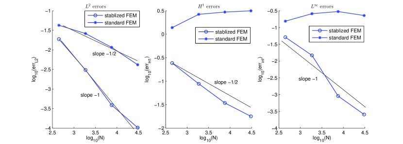
Fig. 3: Discretization errors for Example 1

Figure 4 shows the computed solutions with the two methods. Since the layer is unresolved, the finite element method (11) produces globally oscillating solution. The stabilized method gives a much better approximation, although the layer is slightly smeared, as is typical for the SUPG method.

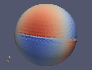
Fig. 4: Example 1: solutions using the stabilized method and the standard method (11).

Example 2.

Now we consider the stationary problem (4) with $c\equiv 0$. The problem is posed on the unit sphere $\Gamma$, with this same velocity field $\mathbf{w}$ as in Example 1. We set $\varepsilon=10^{-6}$, and consider the solution

$$u(\mathbf{x})=\frac{x_{1}x_{2}}{\pi}\mathrm{arctan}\left(\frac{x_{3}}{\sqrt{\varepsilon}}\right).$$

The corresponding right-hand side function $f$ is now given by

$$f(\mathbf{x})=\frac{8\varepsilon^{3/2}(2+\varepsilon+2x_{3}^{2})x_{1}x_{2}x_{3}}{\pi(\varepsilon+4x_{3}^{2})^{2}}+\frac{6\varepsilon x_{1}x_{2}+\sqrt{x_{1}^{2}+x_{2}^{2}}(x_{1}^{2}-x_{2}^{2})}{\pi}\mathrm{arctan}\left(\frac{x_{3}}{\sqrt{\varepsilon}}\right).$$

Note that for $c=0$ one looses explicit control of the $L_{2}$ norm in $\|\cdot\|_{\ast}$. Thus we consider the streamline diffusion error :

$$err_{SD}=\|\mathbf{w}_{\Gamma}\cdot\nabla_{\Gamma}(u-u_{h})\|_{L^{2}(D)}.$$

Results for this error quantity and for $err_{L^{inf}}=\|u-u_{h}\|_{L^{\infty}(D)}$ are shown in Figure 5. We observe a $\mathcal{O}(h)$ behavior for the streamline diffusion error, which is consistent with our theoretical analysis. The $L^{\infty}$-norm of the error also shows a first order of convergence.

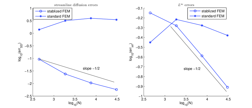
Fig. 5: Discretization errors for Example 2

Example 3.

We show how this stabilization can be applied to a time dependent problem and illustrate its stabilizing effect. We consider a non-stationary problem (3) posed on the torus

$$\Gamma=\{(x_{1},x_{2},x_{3})\ |\ (\sqrt{x_{1}^{2}+x_{2}^{2}}-1)^{2}+x_{3}^{2}=\frac{1}{16}\}.$$ (76)

We set $\varepsilon=10^{-6}$ and define the advection field

$$\mathbf{w}(\mathbf{x})=\frac{1}{\sqrt{x_{1}^{2}+x_{2}^{2}}}(-x_{2},x_{1},0)^{T},$$

which is divergence free and satisfies $\mathbf{w}\cdot\mathbf{n}_{\Gamma}=0$. The initial condition is

$$u_{0}(\mathbf{x})=\frac{x_{1}x_{2}}{\pi}\mathrm{arctan}\left(\frac{x_{3}}{\sqrt{\varepsilon}}\right).$$

The function $u_{0}$ possesses an internal layer, as shown in Figure 6(a).

The stabilized spatial semi-discretization of (3) reads: determine $u_{h}=u_{h}(t)\in V_{h}^{\Gamma}$ such that

$$m(\partial_{t}u_{h},v_{h})+\hat{a}_{h}(u_{h},v_{h})=0\quad\text{for all}~{}~{}v_{h}\in V_{h}^{\Gamma}.$$ (77)

with

$$m(\partial_{t}u,v):= \int_{\Gamma_{h}}\partial_{t}uv\,\mathrm{d}\mathbf{s}+\sum_{T\in\mathcal{F}_{h}}\delta_{T}\int_{T}\partial_{t}u(\mathbf{w}^{e}\cdot\nabla_{\Gamma_{h}}v)\,\mathrm{d}\mathbf{s},$$

$$\hat{a}_{h}(u,v):= \varepsilon\int_{\Gamma_{h}}\nabla_{\Gamma_{h}}u\cdot\nabla_{\Gamma_{h}}v\,\mathrm{d}\mathbf{s}+\frac{1}{2}\left[\int_{\Gamma_{h}}(\mathbf{w}^{e}\cdot\nabla_{\Gamma_{h}}u)v\,\mathrm{d}\mathbf{s}-\int_{\Gamma_{h}}(\mathbf{w}^{e}\cdot\nabla_{\Gamma_{h}}v)u\,\mathrm{d}\mathbf{s}\right]$$

$$+\sum_{T\in\mathcal{F}_{h}}\delta_{T}\int_{T}(-\varepsilon\Delta_{\Gamma_{h}}u+\mathbf{w}^{e}\cdot\nabla_{\Gamma_{h}}u)\mathbf{w}^{e}\cdot\nabla_{\Gamma_{h}}v\,\mathrm{d}\mathbf{s}.$$

Note that $\hat{a}_{h}(\cdot,\cdot)$ is the same as $a_{h}(\cdot,\cdot)$ in (13) with $c\equiv 0$. The resulting system of ordinary differential equations is discretized in time by the Crank-Nicolson scheme.

For $\varepsilon=0$ the exact solution is the transport of $u_{0}(\mathbf{x})$ by a rotation around the $x_{3}$ axis. Thus the inner layer remains the same for all $t>0$. For $\varepsilon=10^{-6}$, the exact solution is similar, unless $t$ is large enough for dissipation to play a noticeable role. The space $V_{h}^{\Gamma}$ is constructed in the same way as in the previous examples. The spatial discretization has 5638 degrees of freedom. The fully discrete problem is obtained by combining the SUPG method in (77) and the Crank-Nicolson method with time step $\delta t=0.1$. The evolution of the solution is illustrated in Figure 6 demonstrating a smoothly ‘rotated’ pattern.

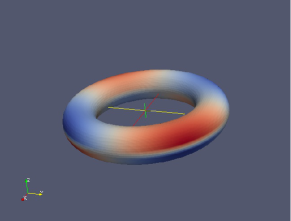
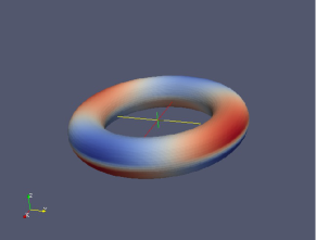
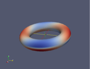
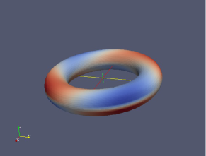
Fig. 6: Example 3: solutions for $t=0,0.6,1.2,1.8$ using the SUPG stabilized FEM.

We repeated this experiment with $\delta_{T}=0$ in the bilinear forms $m(\cdot,\cdot)$ and $\hat{a}_{h}(\cdot,\cdot)$ in (77), i.e. the method without stabilization. As expected, we obtain (on the same grid) much less smooth discrete solutions (Figure 7).

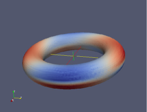
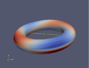
Fig. 7: Example 3: solutions for $t=1.2,1.8$ using the standard FEM.

Remark 4.1.

With respect to mass conservation of the scheme we note the following. For $v_{h}\equiv 1$ in (77) we get, with $M_{h}(t):=\int_{\Gamma_{h}}u_{h}(x,t)\,\mathrm{d}\mathbf{s}$,

$$|\frac{d}{dt}M_{h}(t)| =|\int_{\Gamma_{h}}\frac{1}{2}\mathbf{w}^{e}\cdot\nabla_{\Gamma_{h}}u_{h}\,\mathrm{d}\mathbf{s}|$$

$$=|-\frac{1}{2}\sum_{E\in\mathcal{E}_{h}}\int_{E}\mathbf{w}^{e}\cdot[\mathbf{m}]u_{h}\,\mathrm{d}\mathbf{s}+\frac{1}{2}\int_{\Gamma_{h}}\mathrm{div}_{\Gamma_{h}}\mathbf{w}^{e}u_{h}\,\mathrm{d}\mathbf{s}|$$

$$\lesssim h^{2}\sum_{E\in\mathcal{E}_{h}}\int_{E}|u_{h}|\,\mathrm{d}\mathbf{s}+Ch\int_{\Gamma_{h}}|u_{h}|\,\mathrm{d}\mathbf{s}.$$

Here we used estimates from Lemmas 3.1 and 3.5. Using Lemma 3.6 we get

$$\sum_{E\in\mathcal{E}_{h}}\int_{E}|u_{h}|\,\mathrm{d}\mathbf{s} \lesssim h^{-\frac{1}{2}}\Big{(}\sum_{E\in\mathcal{E}_{h}}\int_{E}u_{h}^{2}\mathrm{d}\mathbf{s}\Big{)}^{\frac{1}{2}}$$

$$\lesssim h^{-1}\big{(}\|u_{h}\|_{L^{2}(\Gamma_{h})}+h\|\nabla_{\Gamma_{h}}u_{h}\|_{L^{2}(\Gamma_{h})}).$$

Assume that for the discrete solution we have a bound $\|u_{h}\|_{L^{2}(\Gamma_{h})}+h\|\nabla_{\Gamma_{h}}u_{h}\|_{L^{2}(\Gamma_{h})}\leq c$ with $c$ independent of $h$. Then we obtain $|\frac{d}{dt}M(t)|\lesssim h$ and thus $|M_{h}(t)-M_{h}(0)|\leq cth$, with a constant $c$ independent of $h$ and $t$. Hence, with respect to mass conservation we have an error that is (only) first order in $h$. Concerning mass conservation it would be better to use a discretization in which in the discrete bilinear form in (13) one replaces

$$\frac{1}{2}\left[\int_{\Gamma_{h}}(\mathbf{w}^{e}\cdot\nabla_{\Gamma_{h}}u)v\,\mathrm{d}\mathbf{s}-\int_{\Gamma_{h}}(\mathbf{w}^{e}\cdot\nabla_{\Gamma_{h}}v)u\,\mathrm{d}\mathbf{s}\right]\quad\text{by}\quad-\int_{\Gamma_{h}}(\mathbf{w}^{e}\cdot\nabla_{\Gamma_{h}}v)u\,\mathrm{d}\mathbf{s}.$$ (78)

This method results in optimal mass conservation: $\frac{d}{dt}M_{h}(t)=0$. It turns out, however, that (with our approach) it is more difficult to analyze. In particular, it is not clear how to derive a satisfactory coercivity bound.

In numerical experiments we observed that the behavior of the two methods (i.e, with the two variants given in (78)) is very similar. In particular, the mass conservation error bound $|M(t)-M(0)|\leq cth$ for the first method seems to be too pessimistic (in many cases). To illustrate this, we show results for the problem described above, but with initial condition

$$u_{0}(\mathbf{x})=1+\frac{1}{\pi}\mathrm{arctan}\left(\frac{x_{3}}{\sqrt{\varepsilon}}\right),\quad\int_{\Gamma}u_{0}\,\mathrm{d}\mathbf{s}=\pi^{2}\approx 9.8696.$$

Figure 8 shows the quantity $M_{h}(t)$ for several mesh sizes $h$. For $t=0$ we have, due to interpolation of the initial condition $u_{0}$, a difference between $M_{h}(0)$ and $\int_{\Gamma}u_{0}\mathrm{d}\mathbf{s}$ that is of order $h^{2}$. For $t>0$ we see, except for the very coarse mesh with $h=1/4$ a very good mass conservation.

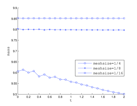
Fig. 8: Total mass variation for Example 3

Example 4.

As a final illustration we show results for the non-stationary problem (3), but now on a surface with a “less regular” shape. We take the surface given in [4]:

$$\Gamma=\{(x_{1},x_{2},x_{3})\ |\ (x_{1}-x_{3}^{2})^{2}+x_{2}^{2}+x_{3}^{2}=1\}.$$ (79)

We set $\varepsilon=10^{-6}$ and define the advection field as the $\Gamma$-tangential part of $\tilde{\mathbf{w}}=(-1,0,0)^{T}.$ This velocity field does not satisfy the divergence free condition. The initial condition is taken as $u_{0}(\mathbf{x})=1.$ We apply the same method as in Example 3. The mesh size is $1/8$ and the time step is $\delta t=0.1$. Figure 9 shows the solution for several $t$ values. We observe that as time evolves mass is transported from the two poles on the right to the left pole, just as expected. Our discretization yields for this strongly convection-dominated transport problem a qualitatively good discrete result, even with a (very) low grid resolution.

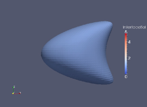
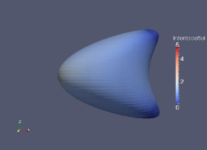
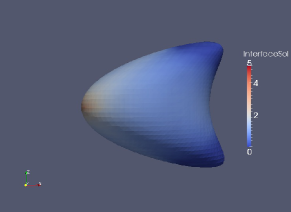
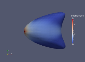
Fig. 9: Example 4: solutions for $t=0,0.5,1.0,2.0$ using the SUPG stabilized FEM.

References

- [1] S. Gross and A. Reusken. Numerical Methods for Two-phase Incompressible Flows, volume 40 of Springer Series in Computational Mathematics. Springer, Heidelberg, 2011.
- [2] M. L. Agrawal and R. Neumann. Surface diffusion in monomolecular films II. experiments and theory. J. Coll. Interface Sci, 121:366–379, 1988.
- [3] H.-G. Roos, M. Stynes, and L. Tobiska. Numerical Methods for Singularly Perturbed Differential Equations — Convection-Diffusion and Flow Problems, volume 24 of Springer Series in Computational Mathematics. Springer-Verlag, Berlin, second edition, 2008.
- [4] G. Dziuk. Finite elements for the Beltrami operator on arbitrary surfaces. In S. Hildebrandt and R. Leis, editors, Partial differential equations and calculus of variations, volume 1357 of Lecture Notes in Mathematics, pages 142–155. Springer, 1988.
- [5] G. Dziuk and C. Elliott. -estimates for the evolving surface finite element method. Math. Comp., 2011. To appear.
- [6] K. Deckelnick, G. Dziuk, C. Elliott, and C.-J. Heine. An -narrow band finite element method for elliptic equations on implicit surfaces. IMA Journal of Numerical Analysis, 30:351–376, 2010.
- [7] M. Bertalmio, G. Sapiro, L.-T. Cheng, and S. Osher. Variational problems and partial differential equations on implicit surfaces. J. Comp. Phys., 174:759–780, 2001.
- [8] M. Olshanskii, A. Reusken, and J. Grande. A finite element method for elliptic equations on surfaces. SIAM J. Numer. Anal., 47:3339–3358, 2009.
- [9] M. Olshanskii and A. Reusken. A finite element method for surface PDEs: matrix properties. Numer. Math., 114:491–520, 2009.
- [10] A. Demlow and M.A. Olshanskii. An adaptive surface finite element method based on volume meshes. SIAM J. Numer. Anal., 50:1624–1647, 2012.
- [11] G. Dziuk and C. Elliott. Finite elements on evolving surfaces. IMA J. Numer. Anal., 27:262–292, 2007.
- [12] S. Sobolev. Some Applications of Functional Analysis in Mathematical Physics. Third Edition. AMS, 1991.
- [13] A. Demlow and G. Dziuk. An adaptive finite element method for the Laplace-Beltrami operator on implicitly defined surfaces. SIAM J. Numer. Anal., 45:421–442, 2007.
- [14] A. Hansbo and P. Hansbo. An unfitted finite element method, based on Nitsche’s method, for elliptic interface problems. Comp. Methods Appl. Mech. Engrg., 191(47–48):5537–5552, 2002.