Phase structure and phase transitions in a three dimensional $\mathrm{SU}(2)$ superconductor

Abstract

We study the three dimensional $\mathrm{SU}(2)$-symmetric noncompact $\text{CP}^{1}$ model, with two charged matter fields coupled minimally to a noncompact Abelian gauge-field. The phase diagram and the nature of the phase transitions in this model have attracted much interest after it was proposed to describe an unusual continuous transition associated with deconfinement of spinons. Previously, it has been demonstrated for various two-component gauge theories that weakly first-order transitions may appear as continuous ones of a new universality class in simulations of relatively large, but finite systems. We have performed Monte-Carlo calculations on substantially larger systems sizes than those in previous works. We find that in some area of the phase diagram where at finite sizes one gets signatures consistent with a single first-order transition, in fact there is a sequence of two phase transitions with an $\mathrm{O}(3)$ paired phase sandwiched in between. We report (i) a new estimate for the location of a bicritical point and (ii) the first resolution of bimodal distributions in energy histograms at relatively low coupling strengths. We perform a flowgram analysis of the direct transition line with rescaling of the linear system size in order to obtain a data collapse. The data collapses up to coupling constants where we find bimodal distributions in energy histograms.

I Introduction

Recently, the $\text{CP}^{1}$ model consisting of two matter fields coupled to an Abelian gauge field has been of great interest in condensed matter physics. One of the sources of interest is the proposed concept of deconfined quantum criticality (DQC). It has been intensively debated as a possible novel paradigm for quantum phase transitions.Senthil et al. (2004a, b); Sandvik (2007); Melko and Kaul (2008); Lou et al. (2009); Sandvik (2010a); Banerjee et al. (2010); Kaul and Sandvik (2012); Motrunich and Vishwanath (2004); Kuklov et al. (2006); Smiseth et al. (2005); Kragset et al. (2006); Motrunich and Vishwanath (2008); Kuklov et al. (2008a); Jiang et al. (2008); Isaev et al. (2010); Nogueira et al. (2007); Kaul and Melko (2008) Such quantum criticality has been suggested to describe phase transitions that would not fit into the Landau-Ginzburg-Wilson (LGW) paradigm of a continuous (second-order) phase transition.Senthil et al. (2004a, b) In particular, the continuous quantum phase transition from an antiferromagnetic Néel state into a paramagnetic valence-bond solid (VBS) state,Read and Sachdev (1989, 1990) does not agree with the LGW-description, according to which two phases with different broken symmetries generically are separated by a first-order phase transition. Recently, evidence for the DQC scenario has been claimed in studies of the so-called $J$-$Q$ model,Sandvik (2007) which is a Heisenberg model with additional higher-order spin interaction terms. Namely, it was suggested that high-precision Quantum Monte Carlo simulations of this model support a continuous Néel - VBS phase transition in accordance with the DQC scenario. Sandvik (2007); Melko and Kaul (2008); Lou et al. (2009); Sandvik (2010a); Banerjee et al. (2010); Kaul and Sandvik (2012)

It has been proposed that the critical field theory of a continuous Néel - VBS phase transition is the so-called noncompact $\text{CP}^{1}$ model ($\text{NCCP}^{1}$), with a $\mathrm{SU}(2)$ symmetric field coupled to a noncompact $\mathrm{U}(1)$ gauge field in three dimensions (3D). Senthil et al. (2004a, b); Motrunich and Vishwanath (2004) Initial efforts on studying this effective model were focused on the special case where the $\mathrm{SU}(2)$ symmetry was broken down to a $\mathrm{U}(1)$$\times$$\mathrm{U}(1)$ symmetry, i.e., the easy-plane limit. For this case, a continuous phase transition was claimed.Motrunich and Vishwanath (2004) However, in Ref. Kuklov et al., 2006, the existence of a paired phase in the $\mathrm{U}(1)$$\times$$\mathrm{U}(1)$ easy-plane action was pointed out. (For earlier discussions of paired phases in various $\mathrm{U}(1)$$\times$$\mathrm{U}(1)$ systems, see Refs. Babaev, 2004; Babaev et al., 2004; Smørgrav et al., 2005; Smiseth et al., 2005.) Furthermore, resorting to mean-field theory arguments, it has been pointed out that at least in the vicinity of a paired state (in the parameter space of the model), the direct phase transition from a symmetric state to a state with broken $\mathrm{U}(1)$$\times$$\mathrm{U}(1)$ symmetry, should be first-order.Kuklov et al. (2006) Subsequent Monte-Carlo calculations have reported a weak first-order phase transition for the easy-plane $\text{NCCP}^{1}$ model.Kuklov et al. (2006); Kragset et al. (2006) The so-called flowgram method has also been introduced in Ref. Kuklov et al., 2006, specifically to characterize weak first-order phase transitions. Using this method, the direct phase transition from a symmetric state to a state with broken $\mathrm{U}(1)$$\times$$\mathrm{U}(1)$ symmetry, has been claimed to be first-order for any non-zero value of the coupling constant. The phase transitions in the easy-plane limit of the $\text{NCCP}^{1}$ model were also extensively studied in variety of other regimes in the context of two-component superconductors with independently conserved condensates.Babaev et al. (2002); Babaev (2004); Babaev et al. (2004); Smiseth et al. (2004); Smørgrav et al. (2005); Smiseth et al. (2005); Herland et al. (2010)

For the $\mathrm{SU}(2)$-symmetric case, Monte Carlo computations have been performed in Ref. Motrunich and Vishwanath, 2004. Here, a direct second-order phase transition was suggested, but the system sizes that were considered were quite small. In a subsequent paper,Motrunich and Vishwanath (2008) an extensive study of the model was performed. In particular, for the direct transition line, a second-order phase transition was claimed. At higher couplings to the gauge field, it was suggested to turn into a first-order transition via a tricritical point. On the other hand, in Ref. Kuklov et al., 2008a (see also Ref. Kuklov et al., 2008b), it was argued that the direct transition line is first-order. The flowgram method employed in Ref. Kuklov et al., 2008a showed no evidence for a tricritical point along the direct transition line. Rather, in this work the large-scale behavior at small couplings to the gauge field was found to be the same as for higher couplings, where indications of a first-order transition were seen by resolving a bimodal distribution in the energy histograms. Note that at the system sizes studied in Ref. Kuklov et al., 2008a, no bimodal distributions were resolved at small coupling constants. Nonetheless, in Ref. Kuklov et al., 2008a, it was concluded that even for weaker couplings, bimodal distributions indicative of a first-order phase transition would emerge for large enough system sizes. This conclusion was based on the similarity of scaling of various quantities for large and small couplings, as evidenced by the flowgrams.

The weakness of the observed first-order phase transition, combined with the necessity of assessing the order of the phase transitions also in the limit of vanishingly small coupling strength, renders this problem computationally extremely demanding. In this work, we therefore examine the phase diagram of the $\text{NCCP}^{1}$ model at substantially larger systems sizes than what has been done in previous works.Motrunich and Vishwanath (2008); Kuklov et al. (2008a) Performing the computations on larger systems allows us to perform a very detailed investigation of the range of parameters where a paired phase is sandwiched in between the fully disordered and fully ordered state. This means that these two phases are separated, not by a direct transition, but by two separate transitions. At small system sizes, these two separate phase transitions in fact give signatures which would lead one to conclude that the system features one single first-order phase transition. The existence of a paired phase sandwiched in between the fully ordered and disordered states emerges only when one considers large enough systems. Our study thus allows us to provide improved estimates for the location of a bicritical point where the direct transition line splits into two.

II Model

The continuum $\text{NCCP}^{1}$ model is written as

where $\beta$ is the inverse temperature and $\bm{\mathbf{\Psi}}^{\dagger}(\bm{\mathbf{x}})=(\psi_{1}^{*}(\bm{\mathbf{x}}),\psi_{2}^{*}(\bm{\mathbf{x}}))$ are two complex fields that are coupled to a noncompact gauge field $\bm{\mathbf{A}}(\bm{\mathbf{x}})$ with charge $e$. The fields $\psi_{c}(\bm{\mathbf{x}})$, $c\in\{1,2\}$, obey the $\text{CP}^{1}$ constraint, $\left|\bm{\mathbf{\Psi}}(\bm{\mathbf{x}})\right|=1$.

The model can be mapped onto a nonlinear $\mathrm{O}(3)$ $\sigma$ model coupled to massive vector fields.Babaev et al. (2002) By introducing the fields,

$$\bm{\mathbf{C}}(\bm{\mathbf{x}})=\frac{\mathrm{i}}{2}\sum_{c}\left[\psi_{c}(\bm{\mathbf{x}})\nabla\psi_{c}^{*}(\bm{\mathbf{x}})-\psi_{c}^{*}(\bm{\mathbf{x}})\nabla\psi_{c}(\bm{\mathbf{x}})\right]-e\bm{\mathbf{A}}(\bm{\mathbf{x}}),$$ (1)

$$\bm{\mathbf{n}}(\bm{\mathbf{x}})=\bm{\mathbf{\Psi}}^{\dagger}(\bm{\mathbf{x}})\bm{\mathbf{\sigma}}\bm{\mathbf{\Psi}}(\bm{\mathbf{x}}),$$ (2)

where the components of $\bm{\mathbf{\sigma}}$ are the Pauli matrices, the $\text{NCCP}^{1}$ model (II) can be rewritten asBabaev et al. (2002)

$$H= \frac{1}{8}[\partial_{\mu}\bm{\mathbf{n}}(\bm{\mathbf{x}})]^{2}+\frac{1}{2}\left[\bm{\mathbf{C}}(\bm{\mathbf{x}})\right]^{2}$$

$$+\frac{1}{2e^{2}}\Bigg{\{}\epsilon_{\mu\nu\lambda}\Big{[}\partial_{\nu}C_{\lambda}(\bm{\mathbf{x}})$$

$$-\frac{1}{4}\bm{\mathbf{n}}(\bm{\mathbf{x}})\cdot\partial_{\nu}\bm{\mathbf{n}}(\bm{\mathbf{x}})\times\partial_{\lambda}\bm{\mathbf{n}}(\bm{\mathbf{x}})\Big{]}\Bigg{\}}^{2},$$ (3)

where sum over repeated indices is assumed. The model represents an $\mathrm{O}(3)$ nonlinear $\sigma$ model coupled to a massive vector field $\bm{\mathbf{C}}(\bm{\mathbf{x}})$. The latter represents a charged mode, and its mass is the inverse magnetic field penetration length. At least for sufficiently large values of electric charge coupling, the model can undergo a Higgs transition (where gauge field becomes massless) without restoring simultaneously any broken global symmetries. In that case, the remaining broken global symmetry is $\mathrm{O}(3)$ which is described by the order parameter $\bm{\mathbf{n}}(\bm{\mathbf{x}})$.

If one introduces an easy-plane anisotropy for the vector field $\bm{\mathbf{n}}(\bm{\mathbf{x}})$, this would break the symmetry of the model to $\mathrm{U}(1)$$\times$$\mathrm{U}(1)$, and the separation of variables yields a neutral and a charged mode, the physics of which has been extensively studied.Babaev et al. (2002); Babaev (2004); Babaev et al. (2004); Smiseth et al. (2004); Smørgrav et al. (2005); Smiseth et al. (2005); Kuklov et al. (2006); Herland et al. (2010) However, there is one substantial difference in the case of $\mathrm{SU}(2)$ symmetry. The charged and neutral sectors are coupled through the last term in Eq. (3). Another difference compared to the $\mathrm{U}(1)$$\times$$\mathrm{U}(1)$ case is that in two dimensions, stable singly quantized vortex lines do not exist in a type-II $\mathrm{SU}(2)$ model (the same applies to vortex lines in three dimensions).Achúcarro and Vachaspati (2000) On the other hand, a type-I $\mathrm{SU}(2)$ model has energetically stable counterparts of ordinary singly quantized type-I vortices. Since composite vortices are topological excitations which lead to the occurrence of paired states in $\mathrm{U}(1)$$\times$$\mathrm{U}(1)$ systems, this aspect makes the phase diagram of $\mathrm{SU}(2)$ theory an especially interesting problem to study.

In the Monte Carlo simulations, we employ a lattice realization of this model on a cubic lattice with size $L^{3}$ and with lattice constant $a=1$. The fields $\psi_{c}(\bm{\mathbf{x}})$ are then defined on the vertices $\bm{\mathbf{r}}\in\{i\bm{\mathbf{\hat{x}}}+j\bm{\mathbf{\hat{y}}}+k\bm{\mathbf{\hat{z}}}|i,j,k\in\{1,\ldots,L\}\}$ of the lattice, $\psi_{c}(\bm{\mathbf{x}})\rightarrow\psi_{c,\bm{\mathbf{r}}}$. For the first term in (II), we rescale the gauge field by $e^{-1}$ and invoke the gauge invariant lattice difference,

$$\left[\frac{\partial}{\partial x_{\mu}}-\mathrm{i}eA_{\mu}(\bm{\mathbf{x}})\right]\psi_{c}(\bm{\mathbf{x}})\rightarrow\psi_{c,\bm{\mathbf{r}}+\bm{\mathbf{\hat{\mu}}}}\,\mathrm{e}^{-\mathrm{i}A_{\mu,\bm{\mathbf{r}}}}-\psi_{c,\bm{\mathbf{r}}},$$ (4)

where $\mu\in\{x,y,z\}$ and $\bm{\mathbf{r}}+\bm{\mathbf{\hat{\mu}}}$ denotes the nearest-neighbor lattice point to vertex $\bm{\mathbf{r}}$ in the $\mu$-direction. The gauge field $A_{\mu,\bm{\mathbf{r}}}$ lives on the $(\bm{\mathbf{r}},\bm{\mathbf{r}}+\bm{\mathbf{\hat{\mu}}})$ links of the lattice. For the Maxwell term we get

$$\left[\bm{\mathbf{\nabla}}\times\bm{\mathbf{A}}(\bm{\mathbf{x}})\right]_{\mu}\to e^{-1}\sum_{\nu,\lambda}\epsilon_{\mu\nu\lambda}\Delta_{\nu}A_{\lambda,\bm{\mathbf{r}}},$$ (5)

where $\Delta_{\nu}$ is the forward finite difference operator, $\Delta_{\nu}A_{\lambda,\bm{\mathbf{r}}}\equiv A_{\lambda,\bm{\mathbf{r}}+\bm{\mathbf{\hat{\nu}}}}-A_{\lambda,\bm{\mathbf{r}}}$, and $\epsilon_{\mu\nu\lambda}$ is the Levi-Civita symbol. In addition, by invoking the $\text{CP}^{1}$ constraint and discarding constant factors in the partition function $Z$, we obtain the following lattice realization of the $\text{NCCP}^{1}$ model:

$$Z=\int\@ifnextchar^{\mathop{\mathcal{\mathstrut D}}\nolimits}\!{\mathop{\mathcal{\mathstrut D}}\nolimits\!}\bm{\mathbf{A}}\int_{0}^{1}\@ifnextchar^{\mathop{\mathcal{\mathstrut D}}\nolimits}\!{\mathop{\mathcal{\mathstrut D}}\nolimits\!}u\int_{0}^{2\uppi}\@ifnextchar^{\mathop{\mathcal{\mathstrut D}}\nolimits}\!{\mathop{\mathcal{\mathstrut D}}\nolimits\!}\theta_{1}\int_{0}^{2\uppi}\@ifnextchar^{\mathop{\mathcal{\mathstrut D}}\nolimits}\!{\mathop{\mathcal{\mathstrut D}}\nolimits\!}\theta_{2}\ \,\mathrm{e}^{-\beta H}$$

$$\begin{aligned} H=\sum_{\bm{\mathbf{r}},\mu}\Bigg{[}&-\sqrt{u_{\bm{\mathbf{r}}}}\sqrt{u_{\bm{\mathbf{r}}+\bm{\mathbf{\hat{\mu}}}}}\cos\left(\Delta_{\mu}\theta_{1,\bm{\mathbf{r}}}-A_{\mu,\bm{\mathbf{r}}}\right)\\ &-\sqrt{1-u_{\bm{\mathbf{r}}}}\sqrt{1-u_{\bm{\mathbf{r}}+\bm{\mathbf{\hat{\mu}}}}}\cos\left(\Delta_{\mu}\theta_{2,\bm{\mathbf{r}}}-A_{\mu,\bm{\mathbf{r}}}\right)\\ &+\frac{1}{2e^{2}}\left(\sum_{\nu,\lambda}\epsilon_{\mu\nu\lambda}\Delta_{\nu}A_{\lambda,\bm{\mathbf{r}}}\right)^{2}\Bigg{]},\end{aligned}$$

where $u_{\bm{\mathbf{r}}}=\left|\psi_{1,\bm{\mathbf{r}}}\right|^{2}=1-\left|\psi_{2,\bm{\mathbf{r}}}\right|^{2}$ and where $\left|\psi_{c,\bm{\mathbf{r}}}\right|$ is the amplitude and $\theta_{c,\bm{\mathbf{r}}}$ is the phase of the complex fields $\psi_{c,\bm{\mathbf{r}}}$.

III Details of the Monte Carlo simulations

The Monte Carlo simulations are performed on a cubic lattice with periodic boundary conditions in all directions and with size $L^{3}$ where $L\in\{8,\dots,96\}$. Up to $4.0\cdot 10^{7}$ sweeps over the lattice were performed for the largest systems, while up to $1.0\cdot 10^{7}$ sweeps were used for initial equilibration and initialization of the coupling distribution (see below). Monte-Carlo time-series were routinely inspected for equilibration. To test for ergodicity, typically $4$ independent large simulations were performed for the largest system sizes. Histograms based on raw data and reweighted data were also compared for consistency. For most of the simulations, the parallel tempering (PT) algorithm was employed.Hukushima and Nemoto (1996); Earl and Deem (2005); Katzgraber (2011) To be specific, we fix the coupling $e$ and perform the computations on a number of replicas (typically from 8 to 32 depending on the system size $L$ and the range of $\beta$ values) in parallel at different values of $\beta$. A Monte Carlo sweep consists of systematically traversing all lattice points with local trial moves of all six field variables by the Metropolis-Hastings algorithm.Metropolis et al. (1953); Hastings (1970) For $u_{\bm{\mathbf{r}}}$, the proposed new values are chosen with uniform probability within the interval $[0,1]$, and for $\theta_{c,\bm{\mathbf{r}}}$, the proposed new values are chosen with uniform probability within the interval $[0,2\uppi\rangle$. For the noncompact gauge field, the proposed new values are chosen within some limited increment (typically $[-\uppi/4,\uppi/4]$) from the old values. There is no gauge fixing involved in the simulations. In addition to these local trial moves, the Monte Carlo sweep also includes a PT trial move of swapping replicas at neighboring $\beta$ values.

All replicas were initially thermalized from an ordered or disordered start configuration. Then, initial runs were performed in order to produce an optimal distribution of couplings for the simulation. In some cases, the set of couplings was found by measuring first-passage-times.Nadler et al. (2008) In this approach, the optimal set of couplings maximizes the flow of replicas in parameter space, essentially by shifting coupling values towards the bottlenecks.Katzgraber et al. (2006) However, in cases with no severe bottleneck, the optimal set of couplings was found by demanding that the acceptance rates for swapping neighboring replicas were equal for all couplings.Hukushima (1999) Irrespective of how the set of couplings was found, it was always ascertained that replicas were able to traverse parameter space sufficiently many times during production runs. The measurements were postprocessed by multiple histogram reweighting.Ferrenberg and Swendsen (1989) Random numbers were generated by the Mersenne-Twister algorithm.Matsumoto and Nishimura (1998) Errors were determined by the jackknife method.Berg (1992)

As mentioned in the introduction, the $\text{NCCP}^{1}$ model is a difficult model on which to perform Monte Carlo computations. In Ref. Kuklov et al., 2008a, the $\text{NCCP}^{1}$ model was mapped to a so-called $J$-current model, which allows simulations based on the worm algorithm.Prokof’ev et al. (1998); Prokof’ev and Svistunov (2001) (For the sake of completeness, and since to our knowledge the details of the mapping have not been published, we present the derivation of this mapping in Appendix A.) An approach based on the $J$-current model was attempted as well. However, due to the presence of long-range interactions in this formulation, it was difficult to work with the lattice sizes above $L\sim 40$. Hence, the computations were performed on the model in the original $\text{NCCP}^{1}$ formulation, using the PT algorithm with which it is easy to grid-parallelize the lattice.

IV Observables and finite-size scaling

Perhaps the most familiar quantity that is used to explore phase transitions, is the specific heat $C_{v}$. The specific heat is given by the second moment of the action,

$$C_{v}=\frac{\beta^{2}}{L^{3}}\left\langle\left(H-\left\langle H\right\rangle\right)^{2}\right\rangle,$$ (6)

where brackets $\langle\dots\rangle$ denote statistical averages. In most cases, $C_{v}$ exhibits a well-defined peak at the phase transition. For a continuous phase transition the correlation length diverges with critical exponent $\nu$ as $\xi\sim\left|t\right|^{-\nu}$, with $t=(\beta-\beta_{\text{c}})/\beta$ being the deviation from the critical coupling $\beta_{\text{c}}$. The critical exponent $\alpha$ is defined by the singular part of $C_{v}$, given by $C_{v}\sim\left|t\right|^{-\alpha}$. Then, in a limited system of size $L^{3}$, the finite-size scaling (FSS) of the specific heat is given by

$$C_{v}\sim C_{0}+C_{1}L^{\alpha/\nu},$$ (7)

where $C_{0}$ and $C_{1}$ are non-universal coefficients. For a first-order transition, with two coexisting phases and no diverging correlation length, there is indeed no critical behavior. Still, first-order transitions exhibit well-behaved FSS with “effective” exponents, $\alpha=1$ and $\nu=1/3$.Fisher and Berker (1982); Cardy and Nightingale (1983) Hence, the peak of the specific heat scales as

$$C_{v}\sim L^{3},$$ (8)

for a first-order transition. Distinguishing between continuous and first-order transitions is an important issue in the present work. For that purpose, FSS of the specific heat peak will play an important role.

We also investigate the third moment of the action given bySudbø et al. (2002); Smiseth et al. (2003)

$$M_{3}=\frac{\beta^{3}}{L^{3}}\left\langle\left(H-\left\langle H\right\rangle\right)^{3}\right\rangle.$$ (9)

In the vicinity of the critical point, this quantity typically features a minimum point and a maximum point [see for instance the inset in panel (b) of Fig. 2]. The difference in the $M_{3}$ value of these two extrema scales as

$$(\Delta M_{3})_{\text{height}}\sim L^{(1+\alpha)/\nu},$$ (10)

and the difference in the coupling values scales as

$$(\Delta M_{3})_{\text{width}}\sim L^{-1/\nu},$$ (11)

for a continuous phase transition. For a first-order transition, the FSS is

$$(\Delta M_{3})_{\text{height}}\sim L^{6},$$ (12)

and

$$(\Delta M_{3})_{\text{width}}\sim L^{-3}.$$ (13)

As was mentioned above, one may construct a three component gauge neutral field $\bm{\mathbf{n}}_{\bm{\mathbf{r}}}$,Babaev et al. (2002) given by

$$\bm{\mathbf{n}}_{\bm{\mathbf{r}}}=\bm{\mathbf{\Psi}}_{\bm{\mathbf{r}}}^{*}\bm{\mathbf{\sigma}}\bm{\mathbf{\Psi}}_{\bm{\mathbf{r}}},$$ (14)

where the components of $\bm{\mathbf{\sigma}}$ are the Pauli matrices. Since it is a unit $\mathrm{O}(3)$ vector, we can introduce a “magnetization”,

$$\bm{\mathbf{M}}=\sum_{\bm{\mathbf{r}}}\bm{\mathbf{n}}_{\bm{\mathbf{r}}}.$$ (15)

The order parameter $\left\langle\bm{\mathbf{m}}\right\rangle$, where $\bm{\mathbf{m}}=\bm{\mathbf{M}}/L^{3}$, signals the onset of order in the $\mathrm{O}(3)$ gauge neutral vector field $\bm{\mathbf{n}}_{\bm{\mathbf{r}}}$, and the critical point of this transition can be accurately determined by a proper analysis of the finite-size crossings of the associated Binder cumulant,Binder (1981a, b); Sandvik (2010b)

$$U_{4}=\frac{5}{2}-\frac{3\langle M^{4}\rangle}{2\langle M^{2}\rangle^{2}}.$$ (16)

The finite-size crossings of the Binder cumulant are known to converge rapidly towards the critical coupling $\beta_{\text{c}}$. Hence, $\beta_{\text{c}}$ can be accurately determined by a simple extrapolation of the finite-size crossings to the thermodynamic limit or by invoking scaling forms that account for finite-size corrections. Beach et al. (2005); Sandvik (2010b)

A number of quantities related to magnetization may be used to extract critical exponents from the Monte Carlo simulations. The magnetic susceptibility, given by

$$\chi=L^{3}\beta\left\langle m^{2}\right\rangle,$$ (17)

when $\beta<\beta_{\text{c}}$, scales as $\chi\sim L^{2-\eta}$ at $\beta=\beta_{\text{c}}$. Hence, we may determine the anomalous scaling dimension $\eta$ by FSS of $\chi$ measurements obtained at $\beta_{\text{c}}$.

The exponent $\nu$ can, alternatively, be determined by calculating the logarithmic derivative of the second power of the magnetization,Ferrenberg and Landau (1991)

$$\frac{\partial}{\partial\beta}\ln\left\langle m^{2}\right\rangle=\frac{\left\langle m^{2}H\right\rangle}{\left\langle m^{2}\right\rangle}-\left\langle H\right\rangle.$$ (18)

The FSS of this quantity is $\frac{\partial}{\partial\beta}\ln\left\langle m^{2}\right\rangle\sim L^{1/\nu}$. Since the logarithmic derivative exhibits a peak that is associated with the critical point, it is possible to extract $\nu$ by measuring the logarithmic derivative at the pseudocritical point, without an accurate determination of $\beta_{\text{c}}$.

Similar to Ref. Motrunich and Vishwanath, 2008, we search for the critical point of the Higgs transition by measuring the dual stiffness

$$\rho_{\text{dual}}^{\mu\mu}(\bm{\mathbf{q}})=\left\langle\frac{\left|\sum_{\bm{\mathbf{r}},\nu,\lambda}\epsilon_{\mu\nu\lambda}\Delta_{\nu}A_{\lambda,\bm{\mathbf{r}}}\,\mathrm{e}^{\mathrm{i}\bm{\mathbf{q}}\bm{\mathbf{r}}}\right|^{2}}{(2\uppi)^{2}L^{3}}\right\rangle,$$ (19)

which is the Fourier space correlator of the magnetic field. This order parameter for the Higgs transition is dual in the sense that it is finite in the high-temperature phase and zero in the low-temperature phase. Like in Ref. Motrunich and Vishwanath, 2008, this quantity is measured at the smallest available wavevector $\bm{\mathbf{q}}\neq\bm{\mathbf{0}}$. We chose to measure $\rho_{\text{dual}}^{zz}$ at $\bm{\mathbf{q}}_{\text{min}}=(2\uppi/L,0,0)$. At the critical point, the quantity $L\rho_{\text{dual}}^{\mu\mu}(\bm{\mathbf{q}}_{\text{min}})$ is universal, such that the finite-size crossings of $L\rho_{\text{dual}}^{\mu\mu}(\bm{\mathbf{q}}_{\text{min}})$ can be used to estimate the critical point of the Higgs transition. In addition, measuring the coupling derivative of $L\rho_{\text{dual}}^{\mu\mu}(\bm{\mathbf{q}}_{\text{min}})$ can be used to estimate the correlation length exponent $\nu$ as

$$\frac{\partial}{\partial\beta}L\rho_{\text{dual}}^{\mu\mu}(\bm{\mathbf{q}}_{\text{min}})\sim L^{1/\nu},$$ (20)

at the critical point.

V Numerical results

V.1 Outline of the phase diagram

The phase diagram of the $\text{NCCP}^{1}$ model is presented in Fig. 1. For small values of $\beta$, there is a normal phase that can be recognized by a disordered gauge neutral vector field $\bm{\mathbf{n}}_{\bm{\mathbf{r}}}$ and a massless gauge field. Hence, $\left\langle m\right\rangle=0$ and $\rho_{\text{dual}}^{\mu\mu}(\bm{\mathbf{q}})\neq 0$ in this phase. For large values of $e$ and higher values of $\beta$, there is a transition into a phase that we label the $\mathrm{O}(3)$ phase. Here, the vector field $\bm{\mathbf{n}}_{\bm{\mathbf{r}}}$ is ordered (the $\mathrm{O}(3)$ symmetry is spontaneously broken), $\left\langle m\right\rangle\neq 0$, whereas the gauge field remains massless, $\rho_{\text{dual}}^{\mu\mu}(\bm{\mathbf{q}})\neq 0$. In the case of $\mathrm{U}(1)\times\mathrm{U}(1)$ symmetric superconductors, this phase is sometimes denoted a metallic superfluid or a paired phase, with long-range order in the gauge neutral linear combination of the phases (in the $\mathrm{U}(1)\times\mathrm{U}(1)$ case), but not in the individual ones.Babaev (2004); Babaev et al. (2004, 2005); Smiseth et al. (2005); Smørgrav et al. (2005); Kuklov et al. (2006); Herland et al. (2010) From the $\mathrm{O}(3)$ phase, by reducing the value of $e$, one enters an ordered phase that we label the $\mathrm{SU}(2)$ phase. Going into this phase, the gauge field dynamically acquires a Higgs mass and the system becomes a two-component $\text{NCCP}^{1}$ superconductor. Note that the Higgs transition is related to a local symmetry, and indeed, is not associated with spontaneous symmetry breaking.Elitzur (1975) This aspect should be kept in mind where we for brevity refer to the fully ordered state as “broken $\mathrm{SU}(2)$” or “fully broken state” to distinguish it from a paired state. The $\mathrm{SU}(2)$ phase is recognized by measuring $\left\langle m\right\rangle\neq 0$ and $\rho_{\text{dual}}^{\mu\mu}(\bm{\mathbf{q}})=0$.

It is generally expected that at small values of $e$, the $\mathrm{SU}(2)$ phase may also be entered directly from the normal phase, i.e., without going through the intermediate paired phase. The nature of the phase transition along this direct transition line in this and related multicomponent models has been intensively debated due to its relevance to deconfined quantum criticality. We will return to the direct transition line in Secs. V.2 and V.3. First, we present results for the two separate transition lines.

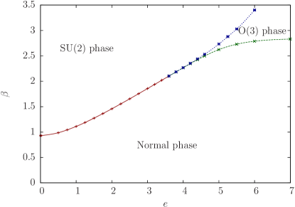
Figure 1: (Color online) Phase diagram of the $\text{NCCP}^{1}$ model. $\mathrm{SU}(2)$ phase: Fully ordered phase where the $\mathrm{O}(3)$ symmetry is spontaneously broken, $\left\langle m\right\rangle\neq 0$, and the gauge field is massive, $\rho_{\text{dual}}^{\mu\mu}(\bm{\mathbf{q}})=0$. $\mathrm{O}(3)$ phase: $\mathrm{O}(3)$ symmetry is spontaneously broken, $\left\langle m\right\rangle\neq 0$, but the gauge field is massless, $\rho_{\text{dual}}^{\mu\mu}(\bm{\mathbf{q}})\neq 0$. Normal phase: $\mathrm{O}(3)$ symmetry is restored, $\left\langle m\right\rangle=0$, and the gauge field is massless, $\rho_{\text{dual}}^{\mu\mu}(\bm{\mathbf{q}})\neq 0$. The direct transition line from the $\mathrm{SU}(2)$ phase to the normal phase is denoted by $+$-markers and a solid red line. The Higgs transition line between the $\mathrm{SU}(2)$ phase and the $\mathrm{O}(3)$ phase is denoted by $\ast$-markers and a dotted blue line. The transition line between the $\mathrm{O}(3)$ phase and the normal phase is denoted by $\times$-markers and a dashed green line. Lines are guide to the eyes.

V.1.1 O(3) line

In Refs. Kuklov et al., 2008a; Kuklov, 2007; Kuklov et al., 2008c, the existence of an intermediate paired phase, separating a fully ordered state from a fully disordered one, was shown in the $\mathrm{SU}(2)$-symmetric theory. The nonlinear $\sigma$ model mapping presented above, suggests that the transition line between the normal phase and the $\mathrm{O}(3)$ phase should be a continuous transition in the $\mathrm{O}(3)$ universality class, at least in the limit far from the bicritical point. We have considered this for the case $e=6.0$, and the FSS results are given in Fig.  2. A log-log plot of the FSS of the peak height in $\frac{\partial}{\partial\beta}\ln\left\langle m^{2}\right\rangle$ is given in panel (a), and the measured peak heights fall on a straight line for $L\geq 20$. The best fit to the form $\frac{\partial}{\partial\beta}\ln\left\langle m^{2}\right\rangle\sim L^{1/\nu}$ yields $\nu=$0.715\pm 0.004$$. In panel (b), we also measure $(\Delta M_{3})_{\text{height}}$, and this quantity exhibits negligible finite-size corrections to scaling at least for $L\geq 10$. The best fit according to Eq. (10) yields $\alpha=$-0.117\pm 0.011$$, where the value of $\nu$ obtained above was used. In this case, it was found that $\nu$ was most precisely determined by measuring the peak height in $\frac{\partial}{\partial\beta}\ln\left\langle m^{2}\right\rangle$ rather than measuring $(\Delta M_{3})_{\text{width}}$. The maximum peak in $M_{3}$ is not very sharp [see the inset of panel (b)]. Thus, the error bars in $(\Delta M_{3})_{\text{width}}$ are large. In order to determine $\eta$, the FSS of the magnetic susceptibility $\chi$ is given in panel (c). Here, $\chi$ is measured at the critical coupling $\beta_{\text{c}}=$2.7894\pm 0.0003$$, which was determined by fitting the Binder crossings of $L$ and $L/2$ to a function that accounts for power-law finite-size corrections. The best fit of $\chi(L)$ was determined for sizes $L\in\{12,\dots,64\}$ to yield $\eta=$0.024\pm 0.014$$. All the exponents listed above correspond well with the exponents of the $\mathrm{O}(3)$ universality class.Holm and Janke (1993); Campostrini et al. (2002)

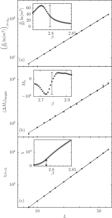
Figure 2: FSS results for the transition between the normal phase and the $\mathrm{O}(3)$ phase when $e=6.0$. 13 system sizes $L\in\{8,\dots,64\}$ are used. In all panels, the solid straight line is the best fit obtained for a fitting function on the form $aL^{b}$ with two free parameters $a$ and $b$. Panel (a): Log-log plot of the maximum in the logarithmic derivative of the second power of the magnetization $(\partial/\partial\beta\ln\langle m^{2}\rangle)_{\beta=\beta_{\text{pc}}}$ [see Eq. (18)] as a function of $L$. The best fit is obtained for sizes $L\in\{20,\dots,64\}$. The inset shows the measure of $(\partial/\partial\beta\ln\langle m^{2}\rangle)_{\beta=\beta_{\text{pc}}}$ in the case when $L=40$. Panel (b): Log-log plot of the third moment height difference $(\Delta M_{3})_{\text{height}}$ as a function of $L$. The best fit is obtained for sizes $L\in\{10,\dots,64\}$. The inset shows the measure $(\Delta M_{3})_{\text{height}}$ in the case when $L=14$. Panel (c): Log-log plot of the magnetic susceptibility measured at the critical coupling $\chi_{\beta=\beta_{\text{c}}}$ as a function of $L$. The best fit is obtained for sizes $L\in\{12,\dots,64\}$. The inset shows $\chi_{\beta=\beta_{\text{c}}}$ for the case when $L=40$, and the arrowheads indicate that $\chi$ is measured at the same fixed coupling $\beta_{\text{c}}$ for all sizes.

V.1.2 Superconducting transition.

Computations have also been performed along the transition line between the $\mathrm{O}(3)$ phase and the $\mathrm{SU}(2)$ phase. In analogy with the paired phase of the $\mathrm{U}(1)$$\times$$\mathrm{U}(1)$ model Babaev (2004); Babaev et al. (2004); Smiseth et al. (2004); Smørgrav et al. (2005); Smiseth et al. (2005); Kuklov et al. (2006); Herland et al. (2010) (i.e., the metallic superfluid), the transition to the $\mathrm{O}(3)$ sector should be associated with the proliferation of single-quanta vortices. In the $\mathrm{U}(1)$$\times$$\mathrm{U}(1)$ model, such vortices have similar phase windings in both complex fields and are topologically well-defined objects. In the $\mathrm{SU}(2)$ case, such vortices can have either similar phase windings in both components, or a phase winding only in one component if the other component exists only in the vortex core of the former. Such objects are non-topological, and are unstable in type-II $\mathrm{SU}(2)$ superconductors.Achúcarro and Vachaspati (2000) This suggests that the system should be a type-I $\mathrm{SU}(2)$ superconductor in order to feature a phase transition into a paired phase. In analogy with single-component type-I superconductors, one would then expect a first-order phase transition.Halperin et al. (1974); Mo et al. (2001) A different viewpoint is based on mean-field arguments, which suggest that the transition line could be a first-order transition line in the vicinity of a bicritical point.Kuklov et al. (2006) Other objects which can disorder the Higgs sector, are HopfionsBabaev et al. (2002); Babaev (2009). In this work we have made no serious attempts at resolving such topological defects.

To check the universality class of this line, FSS results of $\partial/\partial\beta[L\rho_{\text{dual}}^{zz}(\bm{\mathbf{q}}_{\text{min}})]$, obtained at the critical point with $e=5.0$, are given in Fig. 3. First, the critical coupling was determined to be $\beta_{\text{c}}=$2.7347\pm 0.0005$$, by considering the crossings of $L\rho_{\text{dual}}^{zz}(\bm{\mathbf{q}}_{\text{min}})$ (see the inset of Fig. 3). Then, the correlation length exponent was estimated to be $\nu=$0.664\pm 0.039$$. This value is consistent with an inverted 3Dxy transition line.Campostrini et al. (2001) We have not been able to resolve a first-order phase transition at this line.

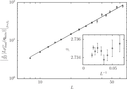
Figure 3: Log-log plot of $\frac{\partial}{\partial\beta}L\rho_{\text{dual}}^{zz}(\bm{\mathbf{q}}_{\text{min}})$ measured at the critical point $\beta_{\text{c}}$, as a function of system size $L$. The charge is $e=5.0$. Measurements are performed for 15 different system sizes $L\in\{8,\dots,64\}$. The derivative was found by calculating the differences of $\rho_{\text{dual}}^{zz}(\bm{\mathbf{q}}_{\text{min}})$. The solid straight line is the best fit obtained with a fit function on the form $aL^{b}$ where $a$ and $b$ are two free parameters. The inset shows the $L\rho_{\text{dual}}^{zz}(\bm{\mathbf{q}}_{\text{min}})$ crossings for systems $L$ and $L/2$ as a function of $L^{-1}$. These crossings were used to estimate the critical point, $\beta_{\text{c}}=$2.7347\pm 0.0005$$. Errors in determining $\beta_{\text{c}}$ are taken into account by also considering the sensitivity of $\nu$ with respect to $\beta$ when estimating the uncertainty in the exponent.

V.2 Estimate for a bicritical point

In Ref. Kuklov et al., 2008a, the flowgram method has been suggested as a useful tool to assess whether or not there is a tricritical point at weak couplings to the gauge field. This method relies on resolving a first-order phase transition at stronger couplings, just below the bicritical point at which the paired phase opens up between the normal phase and the $\mathrm{SU}(2)$ phase. It is thus important to be able to determine the bicritical point accurately. For this purpose, we will focus on the region slightly above the bicritical point and establish when two separate phase transitions are clearly resolved. In this way, we can determine an upper bound on the bicritical point.

V.2.1 Signatures of an intermediate paired phase at $e=4.2$.

In order to discern two separate, but close-lying phase transitions, we need to establish signatures that can be taken as evidence for splitting of a transition line. To this end, results are presented for the case when $e=4.2$. We find unambiguous evidence for two separate phase transitions. Remarkably, at smaller system sizes we find characteristics of the phase transition consistent with a first order transition, and it was interpreted as such in Ref. Kuklov et al., 2008a. ($e=4.2$ corresponds to $g\approx 1.88$ in the units of Ref. Kuklov et al., 2008a. This Reference gave the estimate for the position of the bicritical point at $g\approx 2.0$.) As we shall see, performing computations on larger systems leads to a different conclusion. The reason is that finite-size effects will disguise the existence of separate transitions and make them appear as one.

In Fig. 4, results are presented for four different observables obtained at 12 different system sizes, $L\in\{8,\dots,56\}$, in a coupling range covering both phase transitions. In panel (a), results for the specific heat are given. When system sizes are small, it is only possible to resolve one peak in the specific heat. However, when $L=40$, it is possible to resolve a bump to the left of the peak. The bump, which corresponds to the $\mathrm{O}(3)$ ordering phase transition, becomes more pronounced when $L$ increases. This behavior suggests that there are two transitions instead of one. Moreover, in the inset of panel (a) we study the scaling of the peak on a log-log scale. When $L$ is small, there is a rather steep and slightly increasing slope. However, at higher values of $L$ there is a definite change in the slope towards smaller values, corresponding to a sudden slowing down in the growth of the peak. This behavior should clearly be associated with resolving separate transitions with increasing $L$.

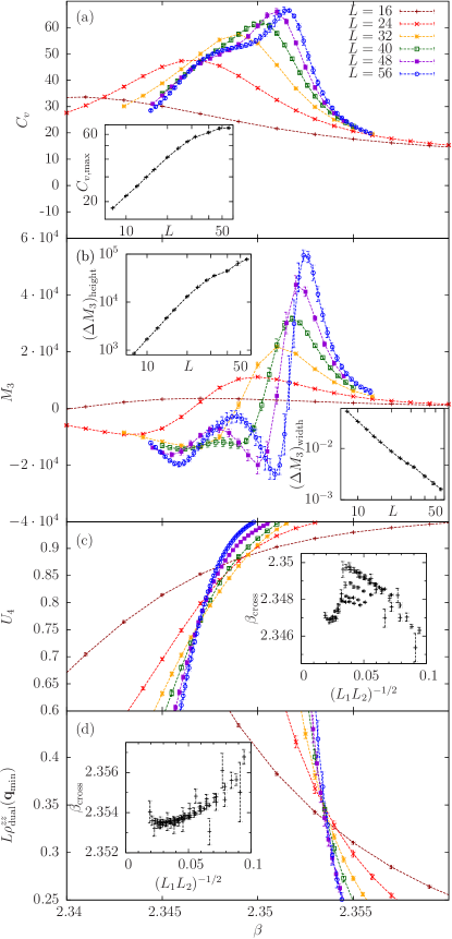
Figure 4: (Color online) Monte Carlo results for four different quantities and 12 different system sizes obtained for a coupling range covering two separate, but close-lying phase transitions. The gauge field coupling $e=4.2$. For clarity, the panels only show results for $L\in\{16,24,32,40,48,56\}$, but insets include all 12 sizes, $L\in\{8,\dots,56\}$. Panel (a) shows results for the specific heat $C_{v}$, and the inset shows the scaling of the peak $C_{v,\text{max}}$ in a log-log scale. Panel (b) shows the results for the third moment of the action $M_{3}$, and the insets show the scaling of $(\Delta M_{3})_{\text{height}}$ and $(\Delta M_{3})_{\text{width}}$ in a log-log scale. Panel (c) shows the Binder cumulant $U_{4}$, and the inset shows the coupling $\beta_{\text{cross}}$ where the Binder curves cross as a function of $(L_{1}L_{2})^{-1/2}$ where $L_{1}$ and $L_{2}$ are the two actual sizes. Panel (d) shows the quantity $L\rho_{\text{dual}}^{zz}(\bm{\mathbf{q}}_{\text{min}})$ and the inset shows the coupling where the curves cross. Lines are guide to the eyes.

In panel (b) of Fig. 4, results for the third moment of the action are presented. When system sizes are small, it is only possible to resolve a characteristic form corresponding to a single phase transition. However, at $L\geq 40$, a secondary form is developing to the left of the original form, resolving the $\mathrm{O}(3)$ ordering transition. When studying the scaling of the quantities $(\Delta M_{3})_{\text{height}}$ and $(\Delta M_{3})_{\text{width}}$ in the insets of the panel, it is clear that they both exhibit slope changes associated with resolving both transitions.

The Binder cumulant is given in panel (c) of Fig. 4, and its crossings are given in the inset of the panel. By considering the crossings with largest $L$, we find that the critical point of the $\mathrm{O}(3)$ ordering transition is $\beta_{\text{c}}=$2.347\pm 0.001$$, a value that corresponds well with the leftmost transition point in panel (a) and (b). Note that there is a non-monotonic behavior in the coupling values of the Binder crossings. Hence, by studying small systems only, one might be misled to overestimate the critical point of the phase transition.

In panel (d) of Fig. 4, we show results for the quantity $L\rho_{\text{dual}}^{zz}(\bm{\mathbf{q}}_{\text{min}})$, and the corresponding crossings are given in the inset. We estimate the critical point of the Higgs transition to be $\beta_{\text{c}}=$2.353\pm 0.001$$ by a crude extrapolation to the thermodynamic limit. Hence, the critical point of the Higgs transition is significantly different from the critical point of the $\mathrm{O}(3)$ ordering transition.

The results in Fig. 4 show that it is of particular importance to simulate large systems in regions where there might be multiple phase transitions in multicomponent gauge theories. Discarding data points for $L>20$, the crossings in panel (c) and (d) appear to converge to the same coupling. In panel (a) and (b), we would only resolve a single phase transition with rather strong thermal signatures.

V.2.2 Monte Carlo results for $e\in\{3.0,\dots,4.6\}$

We first turn our attention to the region with $e<4.2$ to look for the signatures that we have established above. Fig. 5 shows the FSS of the peak in the heat capacity for $e\in\{3.0,\dots,4.2\}$. The results show that there is a definite change in the slope of the scaling of $C_{v,\text{max}}$, also for $e=4.0$ and $3.8$. Note that this signature of splitting appears at higher $L$ when $e$ is reduced, corresponding to the coupling difference between the two transitions being smaller. The slope of the dotted line in Fig. 5 is the slope of a first-order transition [see Eq. (8)]. For all values of $e$ in Fig. 5, we find that for small and intermediate $L$ the slope is steep and increasing, and one might be tempted to conclude that they all are first-order transitions. However, the change towards a smaller slope, that we find for large $L$ and $e\in\{3.8,4.0,4.2\}$, is indeed inconsistent with a single first-order phase transition.

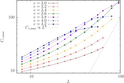
Figure 5: (Color online) Log-log plot of the value of the specific heat peak $C_{v,\text{max}}$ as a function of system size $L$ for seven different values of $e\in\{3.0,\dots,4.2\}$. The dotted line corresponds to the slope expected for a first-order transition, according to Eq. (8). For $e\geq 3.8$, the scaling of $C_{v,\text{max}}$ shows a negative curvature, instead of curving up towards the first-order characteristic scaling line. From this, our upper bound on the position of the bicritical point in the phase diagram would be $e=3.8$. Lines are guide to the eyes.

In Fig. 6, we show the FSS of $(\Delta M_{3})_{\text{height}}$ and $(\Delta M_{3})_{\text{width}}$. Observe that the same signatures of splitting appears for $e\in\{3.8,4.0\}$ as found for $e=4.2$ above, namely that the slope of $(\Delta M_{3})_{\text{height}}$ changes to a smaller value and the slope of $(\Delta M_{3})_{\text{width}}$ changes to a higher value. This is again inconsistent with the scaling of a single first-order transition. For a first-order transition the slopes should converge towards the scaling for first-order transitions, given in Eqs. (12) and (13) (see Ref. Kragset et al., 2006 for an example).

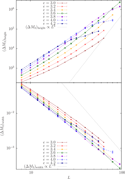
Figure 6: (Color online) Log-log plot of the FSS of the height (upper panel) and the width (lower panel) of the third moment of the action, for seven different values of $e\in\{3.0,\dots,4.2\}$. The dotted lines correspond to the slope expected for a first-order transition, according to Eqs. (12) and (13). Lines are guide to the eyes.

To determine the positions of the $\mathrm{O}(3)$ ordering transition and the Higgs transition, the finite size crossings of $U_{4}$ and $L\rho_{\text{dual}}^{zz}(\bm{\mathbf{q}}_{\text{min}})$ are given in Fig. 7 for eight different values of $e\in\{3.2,\dots,4.6\}$. For $e\in\{4.0,\dots,4.6\}$, the $U_{4}$ crossings and the $L\rho_{\text{dual}}^{zz}(\bm{\mathbf{q}}_{\text{min}})$ crossings clearly extrapolates to different couplings as expected for two separate transitions. Also note the corresponding non-monotonic behavior for the Binder crossings. When the coupling difference between the two phase transitions decreases, larger systems are needed to resolve this feature. For $e=3.8$, we observe that the leftmost $U_{4}$ crossing ($L_{1}=80,L_{2}=96$) deviates, consistent with the non-monotonic behavior for the larger $e$ values. For the sizes available, the crossings seem to converge to the same coupling value for $e\in\{3.2,\dots,3.6\}$.

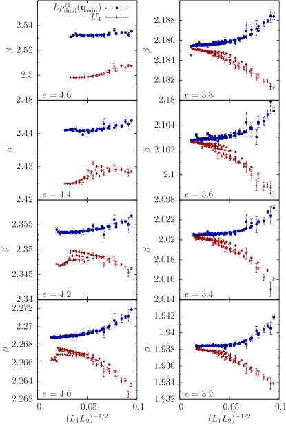
Figure 7: (Color online) Plots of the finite size crossings of the Binder cumulant $U_{4}$ [Eq. (16)], and the quantity $L\rho_{\text{dual}}^{zz}(\bm{\mathbf{q}}_{\text{min}})$ for eight different values of $e\in\{3.2,\dots,4.6\}$. The x-values are given by $(L_{1}L_{2})^{-1/2}$ where $L_{1}$ and $L_{2}$ are the two sizes that form the crossing.

The results in Figs. 5, 6 and 7, show that there are two separate transitions when $e\geq 3.8$. We thus estimate that the bicritical point must be below $e=3.8$. Clearly, the system sizes we are able to reach are too small to conclusively determine if there are separate transitions for $e<3.8$. However, in order to estimate the bicritical point $e_{\text{bc}}$, in Fig. 8 we show results for the coupling difference between the two phase transitions $\Delta\beta_{\text{c}}$ as a function of the coupling $e$. To estimate when $\Delta\beta_{\text{c}}\rightarrow 0$, in the lower panel, we show $\Delta\beta_{\text{c}}$ as a function of $e-e^{*}$ on a log-log scale where $e^{*}$ is some trial value as labeled in the key of the figure. If $e^{*}\approx e_{\text{bc}}$, a straight line should be expected. A positive curvature suggests that $e^{*}>e_{\text{bc}}$ and a negative curvature suggests that $e^{*}<e_{\text{bc}}$. Since there is a clear positive curvature both for $e=3.8$ and $e=3.6$, this suggests that $e_{\text{bc}}<3.6$. Note that the results given in the lower panel of Fig. 8 essentially is an extrapolation of the difference $\Delta\beta_{\text{c}}$ (which also is an extrapolation) in the upper panel to find the point $e_{\text{bc}}$ where $\Delta\beta_{\text{c}}=0$. As it will be clear below, even at the largest system sizes accessible for us, we could not prove that there is a single first-order transition at $e=3.6$. Therefore, simulations of even larger systems are needed to determine more accurately the existence and the position of $e_{\text{bc}}$.

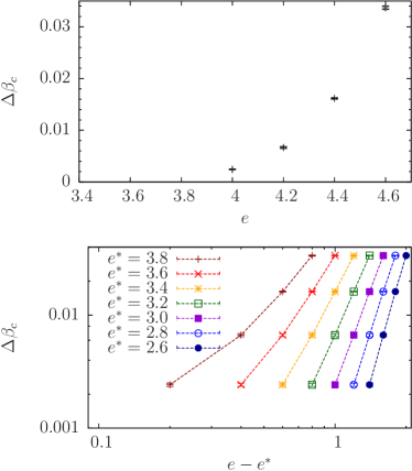
Figure 8: (Color online) Plot of the difference in the critical coupling between the Higgs transition and the $\mathrm{O}(3)$ ordering transition, $\Delta\beta_{c}$. $\Delta\beta_{c}$ is determined by calculating the difference between the $L\rho_{\text{dual}}^{zz}(\bm{\mathbf{q}}_{\text{min}})$ crossing and the $U_{4}$ crossing, and averaging over four of these differences with largest value of $(L_{1}L_{2})^{1/2}$ (i.e., the four leftmost data points from the panels in Fig. 7). We only include results for $e\geq 4.0$ where the non-monotonic behavior of the Binder crossings can clearly be resolved. Upper panel: $\Delta\beta_{c}$ as a function of $e$. Lower panel: Log-log plot of $\Delta\beta_{c}$ as a function of $e-e^{*}$ where $e^{*}$ is given in the key. Positive curvature suggests that $e^{*}>e_{\text{bc}}$, negative curvature suggests that $e^{*}<e_{bc}$ and a straight line suggests that $e^{*}\approx e_{\text{bc}}$. Lines are guide to the eyes.

Our estimates for the bicritical point differ from the results in Refs. Motrunich and Vishwanath, 2008 and Kuklov et al., 2008a which studied substantially smaller systems. Our upper bound $e_{\text{bc}}<3.8$ corresponds to $\mathcal{K}_{\text{bc}}>0.151$ in Ref. Motrunich and Vishwanath, 2008. This means that a part of the line that was interpreted as a direct first-order transition in that work, in fact are two separate transitions. Moreover, the upper bound $e_{\text{bc}}<3.8$ corresponds to $g_{\text{bc}}<1.65$ in Ref. Kuklov et al., 2008a where the bicritical point was estimated to $g\approx 2.0$.

V.2.3 Signatures of a weak first-order transition

Although we are led to a different conclusion concerning the phase diagram than Refs. Motrunich and Vishwanath, 2008 and Kuklov et al., 2008a for $e\geq 3.8$, we find some of the same thermal signatures. As mentioned above (see Figs. 5 and 6), when systems are too small to resolve two phase transitions, the Monte Carlo results show that the scaling of $C_{v,\text{max}}$ and $(\Delta M_{3})_{\text{height}}$ are almost as one would expect for a single first-order transition. Moreover, when investigating the energy distributions for $e\in\{3.8,4.0\}$ in Fig. 9, we find that the histograms are broad. Also, in contrast to previous works, we have resolved bimodal structures for $e\in\{3.4,3.6\}$. This could be interpreted as evidence of a first order phase transition. At the same time we note that they only appear at the largest system sizes. Thus, it is difficult to determine if the correct scaling for first-order transition is obeyed.Lee and Kosterlitz (1990, 1991) The histograms that appear at the largest system sizes, have not yet started to evolve into distributions resembling delta functions. In particular, for the system sizes which we can access the dips in between the peaks are still increasing with system size, rather than decreasing. The latter is required for drawing a firm conclusion that there is a direct first-order phase transition at $e=3.4$ and $e=3.6$. Although rare, there are examples in the literature where bimodal energy distributions are found in cases with no first-order phase transition.Schreiber and Adler (2005); Behringer and Pleimling (2006); Fytas et al. (2008); Jin et al. (2012)

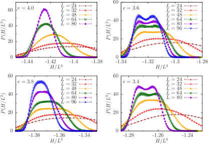
Figure 9: (Color online) Histograms of the probability distribution of the energy per site $H/L^{3}$, for $e\in\{3.4,3.6,3.8,4.0\}$. In every case the flattest (or most bimodal) energy histograms were found by reweighting in the vicinity of the pseudocritical coupling corresponding to the peak of the specific heat, $C_{v,\text{max}}$. The areas under the curves are normalized to unity.

For $e=3.8$, we do not resolve any bimodality, but the histograms are wide. The width of the histograms decreases and the flat top structure disappears when $L$ increases. This is not consistent with a single first-order transition. Note that if this point is located slightly above the bicritical point, then according to a mean-field argument, the Higgs transition should be first-order.Kuklov et al. (2006); Motrunich and Vishwanath (2008) Also, as mentioned above, the instability of composite vortices in type-II $\mathrm{SU}(2)$ theory suggests that the system should be a type-I superconductor in the proximity of the paired phase (since the paired phase results from proliferation of composite vortices), with a possibility of a first order transition via Halperin-Lubensky-Ma mechanism. We did not consider large enough system sizes to resolve this issue.

Combining the results in Figs. 5, 6 and 9, it appears that for couplings slightly above the estimated bicritical point, there are strong thermal signatures in terms of broad energy distributions and rapidly increasing peaks in the specific heat and the third moment of the action. However, when system sizes are larger, we can explicitly see signatures of splitting for $e\geq 3.8$. We cannot exclude the possibility that this may also be the case for some of the couplings with $e<3.8$. Indeed, the crude extrapolation in Fig. 8 suggests that $e=3.6$ also is above the bicritical point. If so, we should expect to see signatures of splitting for system sizes larger than those available in this work. On the other hand, the strong thermal signatures we find for $e<3.8$ can also be consistent with a weak single first-order transition. In that case, we should expect to see that proper first-order scaling is obeyed for larger system sizes.

Summarizing this part, we find that the strongest signatures for a single first-order phase transition were found at $e=3.4$ and $e=3.6$. Previous works on smaller systems did not resolve bimodal structure at these couplings. For $e<3.4$, we did not find any bimodal structure in the energy histograms at the system sizes which we can reach.

V.3 The flowgram method

To analyze situations where it is difficult to resolve and analyze bimodal structures in histograms such as those considered above, the authors of Ref. Kuklov et al., 2006 proposed the flowgram method. By rescaling the linear system size $L\rightarrow C(g)L$, where $g=e^{2}/(4\beta)$ and where $C(g)$ is a monotonous scaling function of the parameter $g$, it may be possible to collapse curves for various physical quantities computed at the phase transition, for different system sizes and coupling constants, onto a single curve.Kuklov et al. (2008b) If such uniform scaling is found for all coupling constants, one may conclude that a phase transition has the same characteristics for all these coupling constants. For instance, if a first order phase transition were to be found for large coupling constants, and the scaled plots fall on a single line for all other coupling constants, one may conclude that the transition is first order for all these coupling constants. To draw such a conclusion, it is very important that a broad enough window of systems sizes $L$ is considered, such that there is adequate overlap of datapoints for all coupling constants, when the data are plotted in terms of $C(g)L$.

In Fig. 10, we show results of a flowgram analysis of the quantity $L\rho_{\text{dual}}^{zz}(\bm{\mathbf{q}}_{\text{min}})$ along the $\mathrm{O}(3)$ ordering transition line. For this analysis, the phase transition is defined to be at the coupling where the Binder cumulant $U_{4}=0.775$. With this definition, we will follow the $\mathrm{O}(3)$ ordering transition line. As mentioned above, $L\rho_{\text{dual}}^{zz}(\bm{\mathbf{q}}_{\text{min}})$ is a universal quantity for a continuous Higgs transition, whereas it will diverge $\sim L$ for a first-order transition. We clearly see such diverging behavior when $e\geq 3.6$ (not shown here) and the FSS is consistent with $L\rho_{\text{dual}}^{zz}(\bm{\mathbf{q}}_{\text{min}})\sim L$. In Refs. Motrunich and Vishwanath, 2008 and Kuklov et al., 2008b, this was interpreted as a first-order phase transition. However, a diverging $L\rho_{\text{dual}}^{zz}(\bm{\mathbf{q}}_{\text{min}})$ is also consistent with being above the bicritical point when following the transition line of the $\mathrm{O}(3)$ ordering transition. Hence, the results in Fig. 10 correspond well with there being two closely separated phase transitions for these values of $e$, see Figs. 4-8 above.

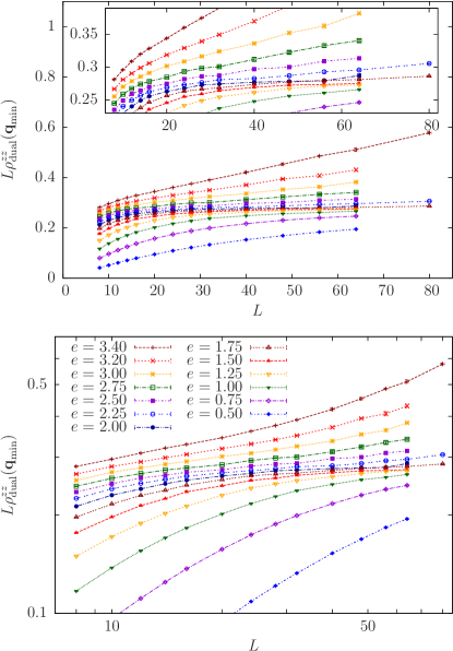
Figure 10: (Color online) Flowgram of $L\rho_{\text{dual}}^{zz}(\bm{\mathbf{q}}_{\text{min}})$ along the $\mathrm{O}(3)$ ordering transition line. In this analysis, the critical point is fixed by $U_{4}=0.775$. Then $L\rho_{\text{dual}}^{zz}(\bm{\mathbf{q}}_{\text{min}})$ is measured at this point and plotted as a function of system size $L$. The results are given for 13 different values of $e\in\{0.5,\dots,3.4\}$. The upper panel shows results on a normal scale and the inset zooms in on the results for $e\in\{1.0,\dots,3.0\}$. The lower panel shows the results on a log-log scale. Lines are guide to the eyes.

For $e\in\{3.0,3.2,3.4\}$, the flowgram analysis suggests that $L\rho_{\text{dual}}^{zz}(\bm{\mathbf{q}}_{\text{min}})$ diverges, but the FSS is weaker than $\sim L$ for the sizes available. This is consistent with either being above the bicritical point, or with a first-order transition. For smaller couplings, the large size behavior of the flowgrams is hard to determine. In particular, for the couplings $e\leq 2.0$ the flowgrams seem to converge slowly to a fixed value, but one cannot rule out diverging behavior at larger sizes.

In Fig. 11, we plot the results for the flowgram data in Fig. 10 in terms of the variable $C(g)L$ on a log-log scale, using the scaling function $C(g)=3.0324g+0.0997[\exp(4.1005g)-1]$. For large values of $C(g)L$, the collapse appears to be good, and consistent with Ref. Kuklov et al., 2008b. In our case, we note that for various couplings there are sizeable finite-size effects which make it impossible to collapse smaller systems onto the same master curve. Removing the data points for the smallest systems for each coupling constant would improve the collapse considerably.

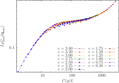
Figure 11: (Color online) Rescaled flowgram of the data in Fig. 10. The system size $L$ is rescaled by $L\rightarrow C(g)L$ where $C(g)=3.0324g+0.0997[\exp(4.1005g)-1]$ with $g=e^{2}/(4\beta)$. Lines are guide to the eyes.

What can the results of Figs. 10 and 11 tell us about the character of the phase transition, and about the existence of a possible tricritical point separating a line of first order phase transitions from a critical line? In Fig. 11, the presence of a tricritical point and a line of second order phase transition would show up as a bifurcations of the master curve at large $C(g)L$. In Ref.  Kuklov et al., 2006, a tricritical point in a global $\mathrm{U}(1)\times\mathrm{U}(1)$ model was detected via a breakdown of the curve collapse just below a tricritical point. We did not observe such a breakdown of the curve collapse for the $\text{NCCP}^{1}$ model. There may exist special cases where the universalities of the line of second order phase transitions and of a tricritical endpoint are quite similar. Then, one may not be able to resolve different plateaus at finite system sizes. In such a situation for large couplings $e$, we would have the behavior shown in Fig. 11. For small couplings, there should appear another horizontal branch of the scaling function at large values of the argument $C(g)L$, were a tricritical point to exist. The results in Fig. 11 show no such feature. However, note that the data points for $e\leq 1.50$ only extend to about the middle of the plateau in Fig. 11. This illustrates the fact, which is also obvious from the lower panel of Fig. 10, that for small couplings $e\leq 1.50$, we have not reached large enough system sizes to be able to ascertain if the curves are horizontal, or if there is an upward curvature in any of the curves for $e\leq 1.50$. Consider for instance the coupling $e=1.50$, which is the curve in Fig. 10 which features the most pronounced horizontal part for the system sizes we have studied. In Fig. 11, this curve extends out to $C(g)L\approx 120$, which is in the middle of the plateau. To ascertain whether this curve falls on the upward curving master curve or continues horizontally would require an extension of the curve out to $C(g)L\approx 400$, or system sizes of about $300^{3}$. No computations have been performed on these types of systems remotely approaching this range. Another way of in principle detecting a tricritical point would be as follows. Suppose that one, in order to get good data collapse for the entire range of coupling constants would need to resort to two different types of scaling functions, one below some coupling constant and another one above this coupling constant. At the point where these functions are joined, one typically has a non-analyticity. One can thus in principal locate a tricritical point at $g=g_{\text{tri}}$ by detecting a non-analyticity in $C(g)$.Kuklov (2012) With our current data we have not resolved such a feature in $C(g)$.

VI Summary

In this work, we have studied the three dimensional $\mathrm{SU}(2)$-symmetric noncompact $\text{CP}^{1}$ model. We have implemented an algorithm which permits us to perform an investigation of the model at substantially larger system sizes than those reached in previous works. It has been shown that at couplings $e=3.8$ and $e=4.0$, which were previously estimated to belong to the regime where the system undergoes a single first-order phase transition, certain signatures should be taken as direct evidence of two separate phase transitions. Hence, we conclude that a bicritical point must be located below $e=3.8$. We find bimodality in histograms, consistent with early stages of development of a first order transition, at $e=3.4$ and $e=3.6$ (though the histograms do not yet resemble two $\delta$-functions and thus indeed it cannot represent a proof of a first order phase transitionKuklov et al. (2008c); Motrunich and Vishwanath (2008); Kuklov et al. (2008a) ) . Although our estimate for the position of bicritical point is different, the data collapse which we find is overall consistent with Ref. Kuklov et al., 2008a.

Appendix A Mapping the $\text{NCCP}^{1}$ model to a $J$-current model

We start with the lattice formulation of the $\text{NCCP}^{1}$ model,

$$S=S_{t}+S_{g},$$ (21)

$$S_{t}\equiv-t\sum_{c,\mu,\bm{\mathbf{r}}}\psi_{c,\bm{\mathbf{r}}}\psi_{c,\bm{\mathbf{r}}+\bm{\mathbf{\hat{\mu}}}}^{*}\,\mathrm{e}^{\mathrm{i}A_{\mu,\bm{\mathbf{r}}}}+\text{c.c.},$$ (22)

$$S_{g}\equiv\frac{1}{8g}\sum_{\mu,\bm{\mathbf{r}}}\left(\sum_{\nu,\lambda}\epsilon_{\mu\nu\lambda}\Delta_{\nu}A_{\lambda,\bm{\mathbf{r}}}\right)^{2},$$ (23)

$$\left|\psi_{1,\bm{\mathbf{r}}}\right|^{2}+\left|\psi_{2,\bm{\mathbf{r}}}\right|^{2}=1\quad\forall\bm{\mathbf{r}},$$ (24)

where we have introduced $t\equiv\beta/2$ and $g\equiv e^{2}/(4\beta)$ – the same coupling constants as in Ref. Kuklov et al., 2008a. Writing the complex fields on polar form,

$$\psi_{c,\bm{\mathbf{r}}}=\rho_{c,\bm{\mathbf{r}}}\,\mathrm{e}^{\mathrm{i}\theta_{c,\bm{\mathbf{r}}}},$$ (25)

$$\int\@ifnextchar^{\mathop{\mathrm{\mathstrut d}}\nolimits}\!{\mathop{\mathrm{\mathstrut d}}\nolimits\!}\psi_{c,\bm{\mathbf{r}}}\@ifnextchar^{\mathop{\mathrm{\mathstrut d}}\nolimits}\!{\mathop{\mathrm{\mathstrut d}}\nolimits\!}\psi_{c,\bm{\mathbf{r}}}^{*}=\int_{0}^{2\uppi}\@ifnextchar^{\mathop{\mathrm{\mathstrut d}}\nolimits}\!{\mathop{\mathrm{\mathstrut d}}\nolimits\!}\theta_{c,\bm{\mathbf{r}}}\int_{0}^{\infty}\rho_{c,\bm{\mathbf{r}}}\@ifnextchar^{\mathop{\mathrm{\mathstrut d}}\nolimits}\!{\mathop{\mathrm{\mathstrut d}}\nolimits\!}\rho_{c,\bm{\mathbf{r}}}$$

we note that the constraint (24) becomes

$${\rho_{1,\bm{\mathbf{r}}}}^{2}+{\rho_{2,\bm{\mathbf{r}}}}^{2}=1,\quad\forall\bm{\mathbf{r}},$$ (26)

which describes the unit circle in the first quadrant of the $\rho_{1,\bm{\mathbf{r}}}\rho_{2,\bm{\mathbf{r}}}$-plane (since $\rho_{c,\bm{\mathbf{r}}}\geq 0$). This means that we can incorporate the constraint directly into the integral by introducing the new field $\phi$,

$$\rho_{1,\bm{\mathbf{r}}}=\cos\phi_{\bm{\mathbf{r}}},\quad\rho_{2,\bm{\mathbf{r}}}=\sin\phi_{\bm{\mathbf{r}}}$$ (27)

$$\left.\prod_{c}\int_{0}^{\infty}\rho_{c,\bm{\mathbf{r}}}\@ifnextchar^{\mathop{\mathrm{\mathstrut d}}\nolimits}\!{\mathop{\mathrm{\mathstrut d}}\nolimits\!}\rho_{c,\bm{\mathbf{r}}}\right|_{\sum_{c}{\rho_{c,\bm{\mathbf{r}}}}^{2}=1}=\int_{0}^{\frac{\uppi}{2}}\cos\phi_{\bm{\mathbf{r}}}\sin\phi_{\bm{\mathbf{r}}}\@ifnextchar^{\mathop{\mathrm{\mathstrut d}}\nolimits}\!{\mathop{\mathrm{\mathstrut d}}\nolimits\!}\phi_{\bm{\mathbf{r}}}$$

such that (LABEL:eq:A_partition_function), (22) and (24) can be replaced by

$$\begin{aligned} S_{t}=-t\sum_{\mu,\bm{\mathbf{r}}}\left[\cos\phi_{\bm{\mathbf{r}}}\cos\phi_{\bm{\mathbf{r}}+\bm{\mathbf{\hat{\mu}}}}\left(\,\mathrm{e}^{\mathrm{i}\left(\theta_{1,\bm{\mathbf{r}}}-\theta_{1,\bm{\mathbf{r}}+\bm{\mathbf{\hat{\mu}}}}+A_{\mu,\bm{\mathbf{r}}}\right)}+\text{c.c.}\right)\right.\\ +\left.\sin\phi_{\bm{\mathbf{r}}}\sin\phi_{\bm{\mathbf{r}}+\bm{\mathbf{\hat{\mu}}}}\left(\,\mathrm{e}^{\mathrm{i}\left(\theta_{2,\bm{\mathbf{r}}}-\theta_{2,\bm{\mathbf{r}}+\bm{\mathbf{\hat{\mu}}}}+A_{\mu,\bm{\mathbf{r}}}\right)}+\text{c.c.}\right)\right].\end{aligned}$$ (28)

Next, we focus on the the $\theta$-dependent part of the integrand, namely $\exp(-S_{t})$, aiming at replacing this field with a $J$-current field. First we symmetrize (28): Assuming periodic boundary conditions and using that

$$A_{\mu,\bm{\mathbf{r}}-\bm{\mathbf{\hat{\mu}}}}=-A_{-\mu,\bm{\mathbf{r}}},$$ (29)

we get

$$S_{t}=-\frac{t}{2}\sum_{\kappa,\bm{\mathbf{r}}}\left[\cos\phi_{\bm{\mathbf{r}}}\cos\phi_{\bm{\mathbf{r}}+\bm{\mathbf{\hat{\kappa}}}}\left(\,\mathrm{e}^{\mathrm{i}\left(\theta_{1,\bm{\mathbf{r}}}-\theta_{1,\bm{\mathbf{r}}+\bm{\mathbf{\hat{\kappa}}}}+A_{\kappa,\bm{\mathbf{r}}}\right)}+\text{c.c.}\right)\right.\\ +\left.\sin\phi_{\bm{\mathbf{r}}}\sin\phi_{\bm{\mathbf{r}}+\bm{\mathbf{\hat{\kappa}}}}\left(\,\mathrm{e}^{\mathrm{i}\left(\theta_{2,\bm{\mathbf{r}}}-\theta_{2,\bm{\mathbf{r}}+\bm{\mathbf{\hat{\kappa}}}}+A_{\kappa,\bm{\mathbf{r}}}\right)}+\text{c.c.}\right)\right],$$ (32)

where $\kappa$ runs over negative as well as positive lattice directions, $\kappa\in\{\pm x,\pm y,\pm z\}$. Then we split $\exp(-S_{t})$ into its individual factors and Taylor expand each of them:

$$\begin{split}\,\mathrm{e}^{-S_{t}}=&\prod_{\kappa,\bm{\mathbf{r}}}\sum_{\begin{subarray}{c}k_{1,\kappa,\bm{\mathbf{r}}}=0\\ l_{1,\kappa,\bm{\mathbf{r}}}=0\end{subarray}}^{\infty}\sum_{\begin{subarray}{c}k_{2,\kappa,\bm{\mathbf{r}}}=0\\ l_{2,\kappa,\bm{\mathbf{r}}}=0\end{subarray}}^{\infty}\\ \Bigg{[}&\frac{\left(\frac{t}{2}\cos\phi_{\bm{\mathbf{r}}}\cos\phi_{\bm{\mathbf{r}}+\bm{\mathbf{\hat{\kappa}}}}\right)^{k_{1,\kappa,\bm{\mathbf{r}}}+l_{1,\kappa,\bm{\mathbf{r}}}}}{k_{1,\kappa,\bm{\mathbf{r}}}!l_{1,\kappa,\bm{\mathbf{r}}}!}\times\\ &\frac{\left(\frac{t}{2}\sin\phi_{\bm{\mathbf{r}}}\sin\phi_{\bm{\mathbf{r}}+\bm{\mathbf{\hat{\kappa}}}}\right)^{k_{2,\kappa,\bm{\mathbf{r}}}+l_{2,\kappa,\bm{\mathbf{r}}}}}{k_{2,\kappa,\bm{\mathbf{r}}}!l_{2,\kappa,\bm{\mathbf{r}}}!}\times\\ &\,\mathrm{e}^{\mathrm{i}(k_{1,\kappa,\bm{\mathbf{r}}}-l_{1,\kappa,\bm{\mathbf{r}}})\left(\theta_{1,\bm{\mathbf{r}}}-\theta_{1,\bm{\mathbf{r}}+\bm{\mathbf{\hat{\kappa}}}}+A_{\kappa,\bm{\mathbf{r}}}\right)}\times\\ &\,\mathrm{e}^{\mathrm{i}(k_{2,\kappa,\bm{\mathbf{r}}}-l_{2,\kappa,\bm{\mathbf{r}}})\left(\theta_{2,\bm{\mathbf{r}}}-\theta_{2,\bm{\mathbf{r}}+\bm{\mathbf{\hat{\kappa}}}}+A_{\kappa,\bm{\mathbf{r}}}\right)}\Bigg{]}\end{split}$$ (33)

The factors of the product over the lattice and directions in (33) may be rearranged such that all the terms containing $\theta_{c,\bm{\mathbf{r}}}$ are collected into one,

$$\,\mathrm{e}^{-S_{t}}=\sum_{\{k,l\}}\prod_{c,\bm{\mathbf{r}}}\,\mathrm{e}^{\mathrm{i}\theta_{c,\bm{\mathbf{r}}}\sum_{\kappa}\left(k_{c,\kappa,\bm{\mathbf{r}}}-l_{c,\kappa,\bm{\mathbf{r}}}-k_{c,\kappa,\bm{\mathbf{r}}-\bm{\mathbf{\hat{\kappa}}}}+l_{c,\kappa,\bm{\mathbf{r}}-\bm{\mathbf{\hat{\kappa}}}}\right)}\\ \times\text{(Everything else)}.$$ (36)

Here $\{k,l\}$ denotes the set of all possible Taylor expansion index field configurations. Inserting this in the partition function (LABEL:eq:A_new_partition_function), the $\theta$-integrals may now be performed. The result is Dirac delta functions (up to an irrelevant scaling factor, which we ignore) at each lattice point, revealing the (“$J$-current”) constraint

$$\sum_{\kappa}k_{c,\kappa,\bm{\mathbf{r}}}-l_{c,\kappa,\bm{\mathbf{r}}}-k_{c,\kappa,\bm{\mathbf{r}}-\bm{\mathbf{\hat{\kappa}}}}+l_{c,\kappa,\bm{\mathbf{r}}-\bm{\mathbf{\hat{\kappa}}}}=0,\quad\forall c,\bm{\mathbf{r}}.$$ (37)

It is convenient to introduce the non-negative bond subcurrents

$$J_{c,\kappa,\bm{\mathbf{r}}}\equiv k_{c,\kappa,\bm{\mathbf{r}}}+l_{c,-\kappa,\bm{\mathbf{r}}+\bm{\mathbf{\hat{\kappa}}}}\in\mathbb{N}_{0},$$ (38)

as well as the total bond currents

$$\quad I_{c,\kappa,\bm{\mathbf{r}}}\equiv J_{c,\kappa,\bm{\mathbf{r}}}-J_{c,-\kappa,\bm{\mathbf{r}}+\bm{\mathbf{\hat{\kappa}}}}\in\mathbb{Z}.$$ (39)

Reordering the sum, the constraint (37) then simplifies to

$$\sum_{\kappa}I_{c,\kappa,\bm{\mathbf{r}}}=0,\quad\forall c,\bm{\mathbf{r}};$$ (40)

the current conservation in each component at each lattice site.

Getting rid of the $\theta$-field we turn our attention to the $\phi$-field. The terms containing $\phi_{\bm{\mathbf{r}}}$ for a given $\bm{\mathbf{r}}$ are on the form

$$\int_{0}^{\frac{\uppi}{2}}\@ifnextchar^{\mathop{\mathrm{\mathstrut d}}\nolimits}\!{\mathop{\mathrm{\mathstrut d}}\nolimits\!}\phi_{\bm{\mathbf{r}}}\cos^{1+2\mathcal{N}_{1,\bm{\mathbf{r}}}}\phi_{\bm{\mathbf{r}}}\sin^{1+2\mathcal{N}_{2,\bm{\mathbf{r}}}}\phi_{\bm{\mathbf{r}}}\times\text{(Everything else)}\\ =\frac{\mathcal{N}_{1,\bm{\mathbf{r}}}!\mathcal{N}_{2,\bm{\mathbf{r}}}!}{2\left(\mathcal{N}_{1,\bm{\mathbf{r}}}+\mathcal{N}_{2,\bm{\mathbf{r}}}+1\right)!}\times\text{(Everything else)},$$ (43)

where, using (38),(39) and (40),

$$\mathcal{N}_{c,\bm{\mathbf{r}}} \equiv\frac{1}{2}\sum_{\kappa}k_{c,\kappa,\bm{\mathbf{r}}}+l_{c,\kappa,\bm{\mathbf{r}}}+k_{c,\kappa,\bm{\mathbf{r}}-\bm{\mathbf{\hat{\kappa}}}}+l_{c,\kappa,\bm{\mathbf{r}}-\bm{\mathbf{\hat{\kappa}}}}$$

$$=\frac{1}{2}\sum_{\kappa}J_{c,\kappa,\bm{\mathbf{r}}}+J_{c,-\kappa,\bm{\mathbf{r}}+\bm{\mathbf{\hat{\kappa}}}}$$

$$=\sum_{\kappa}J_{c,\kappa,\bm{\mathbf{r}}}\in\mathbb{N}_{0}.$$ (44)

The Taylor expansion (33) contains an index field dependent factor as well,

$$\sum_{\{k,l\}}\prod_{c,\kappa,\bm{\mathbf{r}}}\frac{\left(\frac{t}{2}\right)^{k_{c,\kappa,\bm{\mathbf{r}}}+l_{c,\kappa,\bm{\mathbf{r}}}}}{k_{c,\kappa,\bm{\mathbf{r}}}!l_{c,\kappa,\bm{\mathbf{r}}}!},$$ (45)

which we want to write as a function of the $J$-subcurrent field instead. It is easy to see that

$$\prod_{c,\kappa,\bm{\mathbf{r}}}\left(\frac{t}{2}\right)^{k_{c,\kappa,\bm{\mathbf{r}}}+l_{c,\kappa,\bm{\mathbf{r}}}}=\prod_{c,\kappa,\bm{\mathbf{r}}}\left(\frac{t}{2}\right)^{J_{c,\kappa,\bm{\mathbf{r}}}}$$ (46)

by reordering the terms in the product. Using the definition (38), as well as some standard combinatorial results, we may rewrite the denominator part of (45) as

$$\sum_{\{k,l\}}\prod_{c,\kappa,\bm{\mathbf{r}}}\frac{1}{k_{c,\kappa,\bm{\mathbf{r}}}!l_{c,\kappa,\bm{\mathbf{r}}}!} =\sum_{\{J\}}\prod_{c,\kappa,\bm{\mathbf{r}}}\sum_{k_{c,\kappa,\bm{\mathbf{r}}}=0}^{J_{c,\kappa,\bm{\mathbf{r}}}}\frac{1}{k_{c,\kappa,\bm{\mathbf{r}}}!(J_{c,\kappa,\bm{\mathbf{r}}}-k_{c,\kappa,\bm{\mathbf{r}}})!}$$

$$=\sum_{\{J\}}\prod_{c,\kappa,\bm{\mathbf{r}}}\frac{1}{J_{c,\kappa,\bm{\mathbf{r}}}!}\sum_{k_{c,\kappa,\bm{\mathbf{r}}}=0}^{J_{c,\kappa,\bm{\mathbf{r}}}}\binom{J_{c,\kappa,\bm{\mathbf{r}}}}{k_{c,\kappa,\bm{\mathbf{r}}}}$$

$$=\sum_{\{J\}}\prod_{c,\kappa,\bm{\mathbf{r}}}\frac{2^{J_{c,\kappa,\bm{\mathbf{r}}}}}{J_{c,\kappa,\bm{\mathbf{r}}}!},$$ (47)

where $\{J\}$ denotes the set of all possible subcurrent configurations. (There is no problem in summing $k$ away, as it is an independent variable, and all other terms in the partition function are exclusively $J$-dependent – as we will see in a moment.) Inserting (46) and (47) into (45) gives

$$\sum_{\{J\}}\prod_{c,\kappa,\bm{\mathbf{r}}}\frac{t^{J_{c,\kappa,\bm{\mathbf{r}}}}}{J_{c,\kappa,\bm{\mathbf{r}}}!},$$ (48)

which is what we desired.

Lastly, we want to integrate out the gauge field. The gauge field dependent factors of (33) are on the form

$$\exp\left[\mathrm{i}\sum_{c,\kappa,\bm{\mathbf{r}}}A_{\kappa,\bm{\mathbf{r}}}\left(k_{c,\kappa,\bm{\mathbf{r}}}-l_{c,\kappa,\bm{\mathbf{r}}}\right)\right]=\exp\left[\mathrm{i}\sum_{c,\mu,\bm{\mathbf{r}}}A_{\mu,\bm{\mathbf{r}}}I_{c,\mu,\bm{\mathbf{r}}}\right].$$ (49)

Note that the summation is over only positive directions on the RHS. (The RHS is found by expanding and reordering the sum in the exponent on the LHS and applying the identity (29) and the bond current definition (39).) Combining (49) with $\exp(-S_{g})$, the total gauge field contribution to the partition function reads (up to an irrelevant scaling factor)

$$\prod_{\mu,\bm{\mathbf{r}}}\int\@ifnextchar^{\mathop{\mathrm{\mathstrut d}}\nolimits}\!{\mathop{\mathrm{\mathstrut d}}\nolimits\!}A_{\bm{\mathbf{r}}}\ \exp\sum_{\mu,\bm{\mathbf{r}}}\Bigg{[}\mathrm{i}A_{\mu,\bm{\mathbf{r}}}\left(I_{1,\mu,\bm{\mathbf{r}}}+I_{2,\mu,\bm{\mathbf{r}}}\right)\\ -(8g)^{-1}\left(\sum_{\nu,\lambda}\epsilon_{\mu\nu\lambda}\Delta_{\nu}A_{\lambda,\bm{\mathbf{r}}}\right)^{2}\Bigg{]}\\ \propto\exp\Bigg{(}-\frac{g}{2}\sum_{\begin{subarray}{c}c,c^{\prime},\\ \mu,\bm{\mathbf{r}},\bm{\mathbf{r}}^{\prime}\end{subarray}}I_{c,\mu,\bm{\mathbf{r}}}V_{\bm{\mathbf{r}},\bm{\mathbf{r}}^{\prime}}I_{c^{\prime},\mu,\bm{\mathbf{r}}^{\prime}}\Bigg{)},$$ (53)

where we have applied the Coulomb gauge $\Delta_{\mu}A_{\mu,\bm{\mathbf{r}}}=0$. $V_{\bm{\mathbf{r}},\bm{\mathbf{r}}^{\prime}}$ is a long range potential given by by the inverse Fourier transform

$$V_{\bm{\mathbf{r}},\bm{\mathbf{r}}^{\prime}}\equiv\mathcal{F}^{-1}\left\{\left[\sum_{\mu}\sin^{2}\left(\frac{q_{\mu}}{2}\right)\right]^{-1}\right\}\left(\bm{\mathbf{r}}-\bm{\mathbf{r}}^{\prime}\right),$$ (54)

where $q_{\mu}$ is the $\mu$ component of the Fourier space wave vector $\bm{\mathbf{q}}$.

Combining everything, (40), (43), (48), and (53), leaving out trivial scaling factors, we end up with

$$Z=\sum_{\{J|\sum_{\kappa}I_{\kappa}=0\}}\left[\prod_{c,\kappa,\bm{\mathbf{r}}}\frac{t^{J_{c,\kappa,\bm{\mathbf{r}}}}}{J_{c,\kappa,\bm{\mathbf{r}}}!}\right]\left[\prod_{\bm{\mathbf{r}}}\frac{\mathcal{N}_{1,\bm{\mathbf{r}}}!\mathcal{N}_{2,\bm{\mathbf{r}}}!}{\left(\mathcal{N}_{1,\bm{\mathbf{r}}}+\mathcal{N}_{2,\bm{\mathbf{r}}}+1\right)!}\right]\exp\Bigg{(}-\frac{g}{2}\sum_{\begin{subarray}{c}c,c^{\prime},\\ \mu,\bm{\mathbf{r}},\bm{\mathbf{r}}^{\prime}\end{subarray}}I_{c,\mu,\bm{\mathbf{r}}}V_{\bm{\mathbf{r}},\bm{\mathbf{r}}^{\prime}}I_{c^{\prime},\mu,\bm{\mathbf{r}}^{\prime}}\Bigg{)},$$ (55)

which is a $J$-current formulation of the $\text{NCCP}^{1}$ model, see also Ref. Kuklov et al., 2008a.

References

- Senthil et al. (2004a) T. Senthil, A. Vishwanath, L. Balents, S. Sachdev, and M. P. A. Fisher, Science 303, 1490 (2004a), arXiv:cond-mat/0311326v1 [cond-mat.str-el] .
- Senthil et al. (2004b) T. Senthil, L. Balents, S. Sachdev, A. Vishwanath, and M. P. A. Fisher, Phys. Rev. B 70, 144407 (2004b), arXiv:cond-mat/0312617v1 [cond-mat.str-el] .
- Sandvik (2007) A. W. Sandvik, Phys. Rev. Lett. 98, 227202 (2007), arXiv:cond-mat/0611343v3 [cond-mat.str-el] .
- Melko and Kaul (2008) R. G. Melko and R. K. Kaul, Phys. Rev. Lett. 100, 017203 (2008), arXiv:0707.2961v2 [cond-mat.str-el] .
- Lou et al. (2009) J. Lou, A. W. Sandvik, and N. Kawashima, Phys. Rev. B 80, 180414 (2009), arXiv:0908.0740v1 [cond-mat.str-el] .
- Sandvik (2010a) A. W. Sandvik, Phys. Rev. Lett. 104, 177201 (2010a), arXiv:1001.4296v2 [cond-mat.str-el] .
- Banerjee et al. (2010) A. Banerjee, K. Damle, and F. Alet, Phys. Rev. B 82, 155139 (2010), arXiv:1002.1375v1 [cond-mat.str-el] .
- Kaul and Sandvik (2012) R. K. Kaul and A. W. Sandvik, Phys. Rev. Lett. 108, 137201 (2012), arXiv:1110.4130v1 [cond-mat.str-el] .
- Motrunich and Vishwanath (2004) O. I. Motrunich and A. Vishwanath, Phys. Rev. B 70, 075104 (2004), arXiv:cond-mat/0311222v2 [cond-mat.str-el] .
- Kuklov et al. (2006) A. Kuklov, N. Prokof’ev, B. Svistunov, and M. Troyer, Annals of Physics 321, 1602 (2006), arXiv:cond-mat/0602466v1 [cond-mat.str-el] .
- Smiseth et al. (2005) J. Smiseth, E. Smørgrav, E. Babaev, and A. Sudbø, Phys. Rev. B 71, 214509 (2005), arXiv:cond-mat/0411761v2 [cond-mat.supr-con] .
- Kragset et al. (2006) S. Kragset, E. Smørgrav, J. Hove, F. S. Nogueira, and A. Sudbø, Phys. Rev. Lett. 97, 247201 (2006), arXiv:cond-mat/0609336v3 [cond-mat.str-el] .
- Motrunich and Vishwanath (2008) O. I. Motrunich and A. Vishwanath, “Comparative study of Higgs transition in one-component and two-component lattice superconductor models,” (2008), arXiv:0805.1494v1 [cond-mat.stat-mech].
- Kuklov et al. (2008a) A. B. Kuklov, M. Matsumoto, N. V. Prokof’ev, B. V. Svistunov, and M. Troyer, Phys. Rev. Lett. 101, 050405 (2008a), arXiv:0805.4334v1 [cond-mat.stat-mech] .
- Jiang et al. (2008) F.-J. Jiang, M. Nyfeler, S. Chandrasekharan, and U.-J. Wiese, J. Stat. Mech.: Theory Exp. 2008, P02009 (2008), arXiv:0710.3926v1 [cond-mat.str-el] .
- Isaev et al. (2010) L. Isaev, G. Ortiz, and J. Dukelsky, Journal of Physics: Condensed Matter 22, 016006 (2010), arXiv:0903.1630v2 [cond-mat.str-el] .
- Nogueira et al. (2007) F. S. Nogueira, S. Kragset, and A. Sudbø, Phys. Rev. B 76, 220403 (2007), arXiv:0708.3633v2 [cond-mat.str-el] .
- Kaul and Melko (2008) R. K. Kaul and R. G. Melko, Phys. Rev. B 78, 014417 (2008), arXiv:0804.2279v1 [cond-mat.str-el] .
- Read and Sachdev (1989) N. Read and S. Sachdev, Phys. Rev. Lett. 62, 1694 (1989).
- Read and Sachdev (1990) N. Read and S. Sachdev, Phys. Rev. B 42, 4568 (1990).
- Babaev (2004) E. Babaev, Nucl. Phys. B 686, 397 (2004), arXiv:cond-mat/0201547v7 [cond-mat.supr-con] .
- Babaev et al. (2004) E. Babaev, A. Sudbo, and N. W. Ashcroft, Nature 431, 666 (2004), arXiv:cond-mat/0410408v1 [cond-mat.supr-con] .
- Smørgrav et al. (2005) E. Smørgrav, E. Babaev, J. Smiseth, and A. Sudbø, Phys. Rev. Lett. 95, 135301 (2005), arXiv:cond-mat/0508286v1 [cond-mat.supr-con] .
- Babaev et al. (2002) E. Babaev, L. D. Faddeev, and A. J. Niemi, Phys. Rev. B 65, 100512 (2002), arXiv:cond-mat/0106152v3 [cond-mat.supr-con] .
- Smiseth et al. (2004) J. Smiseth, E. Smørgrav, and A. Sudbø, Phys. Rev. Lett. 93, 077002 (2004), arXiv:cond-mat/0403417v4 [cond-mat.supr-con] .
- Herland et al. (2010) E. V. Herland, E. Babaev, and A. Sudbø, Phys. Rev. B 82, 134511 (2010), arXiv:1006.3311v1 [cond-mat.supr-con] .
- Kuklov et al. (2008b) A. B. Kuklov, M. Matsumoto, N. V. Prokof’ev, B. V. Svistunov, and M. Troyer, “Comment on “comparative study of higgs transition in one-component and two-component lattice superconductor models,” (2008b), arXiv:0805.2578v1 [cond-mat.stat-mech].
- Achúcarro and Vachaspati (2000) A. Achúcarro and T. Vachaspati, Physics Reports 327, 347 (2000), arXiv:hep-ph/9904229v2 .
- Hukushima and Nemoto (1996) K. Hukushima and K. Nemoto, J. Phys. Soc. Jpn. 65, 1604 (1996), arXiv:cond-mat/9512035v1 .
- Earl and Deem (2005) D. J. Earl and M. W. Deem, Phys. Chem. Chem. Phys. 7, 3910 (2005), arXiv:physics/0508111v2 [physics.comp-ph] .
- Katzgraber (2011) H. G. Katzgraber, “Introduction to monte carlo methods,” (2011), arXiv:0905.1629v3 [cond-mat.stat-mech].
- Metropolis et al. (1953) N. Metropolis, A. W. Rosenbluth, M. N. Rosenbluth, A. H. Teller, and E. Teller, J. Chem. Phys. 21, 1087 (1953).
- Hastings (1970) W. K. Hastings, Biometrika 57, 97 (1970).
- Note (1) In practice, we discretize the domain of the field variables into a large number of bins, , in order to speed up the computations by the use of lookup tables. We use in the simulations, which we believe to be sufficiently large to render the simulation results indistinguishable from the continuum limit. Test simulations with other values support this claim.
- Nadler et al. (2008) W. Nadler, J. H. Meinke, and U. H. E. Hansmann, Phys. Rev. E 78, 061905 (2008).
- Katzgraber et al. (2006) H. G. Katzgraber, S. Trebst, D. A. Huse, and M. Troyer, J. Stat. Mech.: Theory Exp. 2006, P03018 (2006), arXiv:cond-mat/0602085v3 [cond-mat.other] .
- Hukushima (1999) K. Hukushima, Phys. Rev. E 60, 3606 (1999), arXiv:cond-mat/9903391v1 [cond-mat.dis-nn] .
- Ferrenberg and Swendsen (1989) A. M. Ferrenberg and R. H. Swendsen, Phys. Rev. Lett. 63, 1195 (1989).
- Matsumoto and Nishimura (1998) M. Matsumoto and T. Nishimura, ACM Trans. Model. Comput. Simul. 8, 3 (1998).
- Berg (1992) B. A. Berg, Comput. Phys. Commun. 69, 7 (1992).
- Prokof’ev et al. (1998) N. Prokof’ev, B. Svistunov, and I. Tupitsyn, Physics Letters A 238, 253 (1998).
- Prokof’ev and Svistunov (2001) N. Prokof’ev and B. Svistunov, Phys. Rev. Lett. 87, 160601 (2001), arXiv:cond-mat/0103146 .
- Fisher and Berker (1982) M. E. Fisher and A. N. Berker, Phys. Rev. B 26, 2507 (1982).
- Cardy and Nightingale (1983) J. L. Cardy and P. Nightingale, Phys. Rev. B 27, 4256 (1983).
- Sudbø et al. (2002) A. Sudbø, E. Smørgrav, J. Smiseth, F. S. Nogueira, and J. Hove, Phys. Rev. Lett. 89, 226403 (2002), arXiv:cond-mat/0207501v2 [cond-mat.str-el] .
- Smiseth et al. (2003) J. Smiseth, E. Smørgrav, F. S. Nogueira, J. Hove, and A. Sudbø, Phys. Rev. B 67, 205104 (2003), arXiv:cond-mat/0301297v2 [cond-mat.str-el] .
- Binder (1981a) K. Binder, Phys. Rev. Lett. 47, 693 (1981a).
- Binder (1981b) K. Binder, Z. Phys. B 43, 119 (1981b).
- Sandvik (2010b) A. W. Sandvik, AIP Conference Proceedings 1297, 135 (2010b), arXiv:1101.3281v1 [cond-mat.str-el] .
- Beach et al. (2005) K. S. D. Beach, L. Wang, and A. W. Sandvik, “Data collapse in the critical region using finite-size scaling with subleading corrections,” (2005), arXiv:cond-mat/0505194v1 [cond-mat.stat-mech] .
- Ferrenberg and Landau (1991) A. M. Ferrenberg and D. P. Landau, Phys. Rev. B 44, 5081 (1991).
- Babaev et al. (2005) E. Babaev, A. Sudbø, and N. W. Ashcroft, Phys. Rev. Lett. 95, 105301 (2005), arXiv:cond-mat/0507605v1 [cond-mat.supr-con] .
- Elitzur (1975) S. Elitzur, Phys. Rev. D 12, 3978 (1975).
- Kuklov (2007) A. Kuklov, (2007), at the Nordita Quantum Fluids workshop, Stockholm, http://www.nordita.org/qf2007/kuklov.pdf.
- Kuklov et al. (2008c) A. B. Kuklov, M. Matsumoto, N. V. Prokof’ev, B. V. Svistunov, and M. Troyer, Bull. Am. Phys. Soc. 53, S12.00006 (2008c).
- Holm and Janke (1993) C. Holm and W. Janke, Phys. Rev. B 48, 936 (1993).
- Campostrini et al. (2002) M. Campostrini, M. Hasenbusch, A. Pelissetto, P. Rossi, and E. Vicari, Phys. Rev. B 65, 144520 (2002), arXiv:cond-mat/0110336v2 [cond-mat.stat-mech] .
- Halperin et al. (1974) B. I. Halperin, T. C. Lubensky, and S.-K. Ma, Phys. Rev. Lett. 32, 292 (1974).
- Mo et al. (2001) S. Mo, J. Hove, and A. Sudbø, Phys. Rev. B 65, 104501 (2001), arXiv:cond-mat/0109260v2 .
- Babaev (2009) E. Babaev, Phys. Rev. B 79, 104506 (2009), arXiv:0809.4468v3 [cond-mat.supr-con] .
- Campostrini et al. (2001) M. Campostrini, M. Hasenbusch, A. Pelissetto, P. Rossi, and E. Vicari, Phys. Rev. B 63, 214503 (2001), arXiv:cond-mat/0010360v1 [cond-mat.stat-mech] .
- Note (2) When is large, such that there are two clearly separate transitions, and are determined by the two extrema of the most prominent transition in the plot, which is the Higgs transition.
- Lee and Kosterlitz (1990) J. Lee and J. M. Kosterlitz, Phys. Rev. Lett. 65, 137 (1990).
- Lee and Kosterlitz (1991) J. Lee and J. M. Kosterlitz, Phys. Rev. B 43, 3265 (1991).
- Schreiber and Adler (2005) N. Schreiber and J. Adler, J. Phys. A 38, 7253 (2005), arXiv:cond-mat/0507394v1 [cond-mat.stat-mech] .
- Behringer and Pleimling (2006) H. Behringer and M. Pleimling, Phys. Rev. E 74, 011108 (2006), arXiv:cond-mat/0606283v1 [cond-mat.stat-mech] .
- Fytas et al. (2008) N. G. Fytas, A. Malakis, and K. Eftaxias, J. Stat. Mech.: Theory Exp. 2008, P03015 (2008), arXiv:0802.0073v3 [cond-mat.stat-mech] .
- Jin et al. (2012) S. Jin, A. Sen, and A. W. Sandvik, Phys. Rev. Lett. 108, 045702 (2012), arXiv:1110.5874v2 [cond-mat.stat-mech] .
- Note (3) This is not the same scaling function as suggested in Ref. \rev@citealpnumKuklov_ArXiv_2008. In that work, the system sizes were smaller than in this work. Because of finite-size effects, the best scaling function may change slightly when larger systems are included. In this context, the best scaling function is determined by requiring the best collapse for the largest system sizes.
- Kuklov (2012) A. B. Kuklov, (2012), private communication.
- Note (4) In Ref. \rev@citealpnumKuklov_PRL_2008, a bimodal distribution was seen for , where we do not observe bimodality. Ref. \rev@citealpnumKuklov_PRL_2008, however, finds bimodality in other quantities than we consider. We have evidence that is above the bicritical point. A previously discussed scenario is that there are also first-order transitions above the bicritical point.