Heating of the magnetic chromosphere: observational constraints from Ca II $\lambda 8542$ spectra

Abstract

The heating of the Sun’s chromosphere remains poorly understood. While progress has been made on understanding what drives the quiet Sun internetwork chromosphere, chromospheric heating in strong magnetic field regions continues to present a difficult challenge, mostly because of a lack of observational constraints. We use high-resolution spectropolarimetric data from the Swedish 1-m Solar Telescope to identify the location and spatio-temporal properties of heating in the magnetic chromosphere. In particular, we report the existence of raised-core spectral line profiles in the Ca II $\lambda 8542$ line. These profiles are characterized by the absence of an absorption line core, showing a quasi-flat profile between $\lambda\approx\pm 0.5$ Å, and are abundant close to magnetic bright-points and plage. Comparison with 3D MHD simulations indicates that such profiles occur when the line-of-sight goes through an "elevated temperature canopy" associated with the expansion with height of the magnetic field of flux concentrations. This temperature canopy in the simulations is caused by ohmic dissipation where there are strong magnetic field gradients. The raised-core profiles are thus indicators of locations of increased chromospheric heating. We characterize the location and temporal and spatial properties of such profiles in our observations, thus providing much stricter constraints on theoretical models of chromospheric heating mechanisms than before.

1. Introduction

The heating of the Sun’s chromosphere requires more than an order of magnitude more mechanical energy flux than the corona and heliosphere combined (Anderson & Athay, 1989; Withbroe & Noyes, 1977). Nevertheless, the heating mechanism powering the chromosphere remains elusive, especially in the magnetic chromosphere in and around network and plage regions (e.g., Judge et al., 2010). This is in part because most studies have focused on quiet-Sun internetwork regions (e.g., Carlsson & Stein, 1997; Straus et al., 2008). In addition, most theoretical studies have avoided detailed comparisons with chromospheric diagnostics, which are most often formed under non-LTE and non-equilibrium conditions and thus difficult to model, instead focusing on simply comparing the energy flux associated with specific physical heating mechanisms (e.g. Goodman & Kazeminezhad, 2010) to the canonical values derived from semi-empirical 1D hydrostatic models of the chromosphere (Vernazza et al., 1981; Fontenla et al., 1993). Such a limited comparison does not properly capture the chromospheric conditions, which are significantly different from the 1D VAL and FAL models (in terms of dynamics and structuring, see, e.g., Carlsson & Stein, 1997).

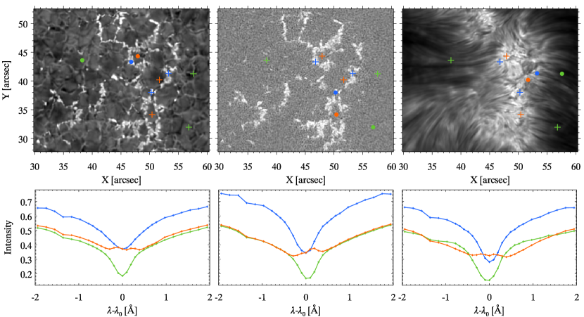
Figure 1.— Ca II $\lambda 8542$ filtergrams (top-row): Stokes $I$ at $-1055$ mÅ from line center (left), Stokes $V$ at the same wavelength (middle) and the line core intensity (right). The color markers indicate the location of hand-picked quiet-Sun profiles (green), RC profiles (orange) and bright-point profiles (blue). The circular markers indicate the location of the intensity profiles shown in each of the panels below (same color coding).

Here we report on new observational constraints on chromospheric heating derived from the Ca II $\lambda 8542$ spectral line. During the past decade, the Ca II infrared (IR) triplet lines ($\lambda 8498$, $\lambda 8542$, $\lambda 8662$) have become popular chromospheric diagnostics in solar studies. In particular, the Ca II $\lambda 8542$ line has been used in a variety of different chromospheric studies, for example, to determine the disk counterpart of spicules (Rouppe van der Voort et al., 2009), analyze the energy flux carried by acoustic waves into the lower atmosphere (Vecchio et al., 2009), study torsional motions in the atmosphere (De Pontieu et al., 2012; Wedemeyer-Böhm et al., 2012), or to carry out spectropolarimetric studies in sunspots (Socas-Navarro et al., 2000; López Ariste et al., 2001; Kleint, 2012).

Cauzzi et al. (2009) suggested a connection between chromospheric heating and the width of the H I $\lambda 6563$ (H$\alpha$) line, which is found to be strongly sensitive to changes in temperature. Furthermore, their maps of the line core intensity of Ca II $\lambda 8542$ show strong similarities with their H$\alpha$ line-width maps. Further support for a relationship between core brightness of Ca lines and elevated temperatures is provided by Henriques (2012), who used the intensity of Ca II $\lambda 3968$ as a measurement of the upper-photospheric temperature.

Although the velocity field and temperature stratification in the solar atmosphere produce an imprint in the spatially-resolved profiles from the Ca II IR lines, they usually remain absorption lines with a conspicuous line core. Interestingly, Pietarila et al. (2007b) report some examples of reversals in the NLTE core of the Ca II $\lambda 8542$ line, which are later associated with elevated chromospheric temperatures in Pietarila et al. (2007a). However the mechanism producing this increase in temperature or the spatio-temporal properties are not investigated. These raised-core (RC hereafter) profiles are found in pixels with intermediate magnetic flux in their observations.

In this letter, we use full-Stokes Ca II $\lambda 8542$ data to show the ubiquity of such RC profiles in the vicinity of strong magnetic fields. We report on the peculiar spatial distribution of the RC profiles, and analyze their spatial and temporal properties to provide constraints on chromospheric heating models. Finally, we propose a scenario that explains the profile shapes, using synthetic spectral line profiles from a 3D radiative MHD simulation.

2. Observations

The observations are of a bipolar active region (AR10998) at approximately $205\arcsec$ heliocentric distance. The datasets were acquired at the Swedish 1-m Solar Telescope (SST) using the CRisp Imaging SpectroPolarimeter (CRISP, Scharmer et al., 2008) on 14 Jun 2008 at 08:36:54.

Our data consists of a 41 minute time-series including 225 full-Stokes line-scans (time steps) of the Ca II $\lambda 8542$ line, with a temporal cadence of 11 seconds. The line was sampled at 29 line positions across the range $\pm 1.94$ Å from the line center, with a spectral sampling of 97 mÅ in the core up to $\pm 0.78$ Å, and 194 mÅ in the outer wings.

The data are processed using the image restoration technique Multi-Object-Multi-Frame-Blind- Deconvolution (MOMFBD, van Noort et al., 2005), which allows to achieve a spatial resolution of $\lambda/D=$0$\farcs$18. Instrumental polarization is compensated using the 2D calibration described in Schnerr et al. (2011) and the SST model at 854 nm from de la Cruz Rodríguez (2010).

We have made extensive use of CRISPEX (Vissers & Rouppe van der Voort, 2012) a tool for the exploration of CRISP datasets.

2.1. The raised-core profiles

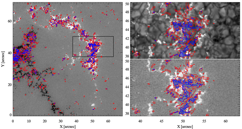
Figure 2.— Spatial distribution of RC profiles measured as number of zero-crossings of ${\rm d}I/{\rm d}\lambda$ over the core region ($\pm 582$ mÅ). The left panel shows a Stokes $V$ map integrated over all 29 line positions with contours delineating areas with 3 (red) and 4 (blue) zero-crossings. The rightmost panels show a zoom-in on the region outlined in the left panel, with a wide-band image as background at the top. An online movie is available.

The observed field-of-view (FOV) contains two patches of network with opposite polarities. In the photosphere, observed in the wings of the $\lambda 8542$ line, the images show granulation with two concentrations of bright-points. In the chromosphere, visible in the core of the line, the images show a landscape of dark elongated fibrils that extend outwards from the network patches.

A section of our FOV is enlarged for clarity in Fig. 1. This patch of mostly unipolar plage shows strong magnetic field concentrations (Stokes $V$, top middle panel) that are tightly correlated with the locations of bright-points (Stokes $I$, top left panel). The line core image (top right panel), which is sensitive to chromospheric plasma, shows fibrils extending from the plage region. The plage region is generally very bright compared with the fibrils.

We distinguish three different “typical” line profiles and give examples from three different locations for each profile type: quiet (locations and spectra marked with green symbols), bright-point (blue symbols) and RC profiles (orange symbols). The quiet profiles show a “classical” Ca II $\lambda 8542$ profile with bright photospheric wings and a chromospheric absorption core (green profiles in bottom row of Fig. 1). The shape of the bright-point profiles (blue in bottom row) is very similar to that of the quiet-Sun profiles but with enhanced intensity for all wavelengths.

The RC profiles look markedly different. The photospheric wings of RC profiles are virtually identical in brightness and shape to those of quiet profiles. However, the chromospheric core of RC profiles is very different: it is almost flat, and much brighter than the core of the quiet profiles. The chromospheric core of RC profiles actually has an intensity that is similar to that of the core of the bright-point profiles.

In a large fraction of the RC profiles, we have also noticed two weak emission lobes at approximately $\lambda=\pm 194$ mÅ from line center. These lobes are further discussed in §§ 2.3 and 3.

2.2. Spatial distribution and ubiquity

One clue to the cause of the RC profiles comes from investigating their spatial distribution and ubiquity in the plage region. Clearly not all locations show RC profiles. To determine, in an automated fashion, the location of RC profiles we tried several approaches. We found that the ratio between core and wing intensities reveals many locations of raised core profiles, but visual inspection shows that it also flags many "false positive" locations (usually narrow absorbing cores that are strongly Doppler-shifted). A better method exploits the fact that around the core of these profiles the intensity is relatively flat with wavelength, so that the derivative of intensity with wavelength $\text{d}I/\text{d}\lambda$ hovers around 0, with frequent changes of the sign of the derivative. We thus developed an algorithm that calculates the number of zero-crossings of $\text{d}I/\text{d}\lambda$ around the core of the line. Both bright-point and quiet profiles have values of 1, whereas RC profiles almost always have larger values.

By overplotting contours of the number of zero-crossings of $\text{d}I/\text{d}\lambda$ (red and blue contours in Fig. 2), we find that the RC profiles are located in the proximity of photospheric bright-points and in extended patches of photospheric granulation, which are embedded in patches of plage. In fact, they are quite rare outside this configuration. This is quite clear from the enlarged regions shown in the right column of Fig. 2. The RC profiles are preferentially located inside the ring of bright-points, with only a few exceptions found outside. Our analysis also shows that these RC profiles are ubiquitous and occur wherever there is plage (or network), with their frequency increasing in more complex regions. The spatial extent of seemingly coherent or contiguous regions with RC profiles is of order a fraction of an arcsecond up to an arcsecond.

2.3. Temporal properties

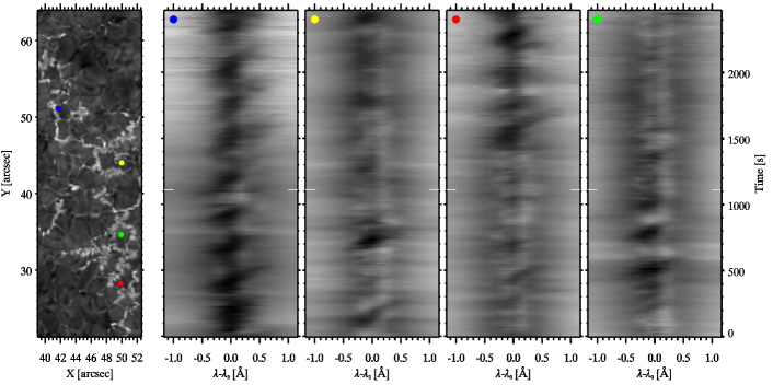
Figure 3.— Temporal evolution and lifetime of the RC profiles. The top row illustrates the temporal evolution of some $\lambda 8542$ profiles at locations indicated with color markers in the top left panel and repeated in each $\lambda-t$ plot (right panels). The second panel from left corresponds to a traditional absorption profile showing a shock induced temporal pattern. The last three panels correspond to the time evolution of three RC profiles. The time of the image in the top-left panel is indicated in the time slices with a yellow marker. The bottom row provides information about the typical timescales that dominate the temporal evolution of the RC profiles: map of the auto-covariance timescale ($8\times$ rebinned) (left) and a histogram of auto-covariance timescales for locations with RC profiles (right), using the original data (dashed-red), $8\times 8$ (solid-black) and $16\times 16$ rebinning (dotted-blue). The vertical black-dotted line indicates the median auto-covariance timescale: 81 seconds.

The temporal behavior of the RC profiles is very different from that of a more typical profile, as can be seen by comparing the three top-right panels with the second panel from the left in the top row of Fig. 3. The latter shows the temporal evolution of the Ca II $\lambda$8542 line profile in a location that does not show strong RC behavior. It is dominated by a succession of magneto-acoustic shocks, visible as strongly absorbing features and similar to those described by Langangen et al. (2008); Vecchio et al. (2009). Two brief moments of RC profiles occur in between shocks. The three RC locations (rightmost panels, top row) on the other hand show raised core emission for much of the time-series, with only occasional shock-induced absorption. The RC profiles are not constant in time but show significant variability. We find that the imprint from the red emission lobe at $\pm 194$ mÅ  is often noticeable throughout the timeseries, which is not always the case for the blue lobe.

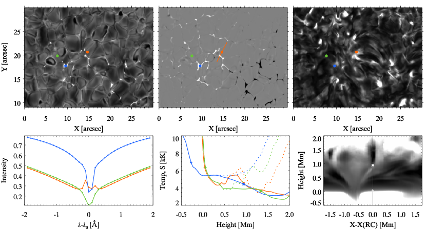
Figure 4.— Synthetic $\lambda 8542$ observations and physical quantities from our 3D MHD simulation. In the top row, monochromatic intensity in the wing (left), the vertical component of the magnetic field at $z=0$ km (middle) and the monochromatic intensity at line center (right). The lower-left panel shows the intensity profiles at locations indicated with colored markers in the top row: quiet-Sun (green), bright-point (blue) and raised-core profile (orange). The lower-middle panel shows the temperature stratification (dashed) and source function (solid) at each location. The markers over-plotted on the source function indicate the height at which $\tau_{\nu}=1$ in the continuum (plus) and at line center (star). The lower right panel shows a 2D cut (along the orange line shown in the top middle panel) of the temperature as a function of height in the simulation. The zero-point in x is at the location of the orange circle in the top middle panel, the site of an RC profile. Markers show the location of $\tau_{\nu}=1$ in the continuum (plus) and at line center (star).

The online movie of Fig. 2 shows evidence of contiguous and/or coherent spatial regions that contain RC profiles with typical spatial and temporal scales of order 0.5″and 1–2 minutes. These regions change shape and move about within the plage region. To determine the typical timescales over which RC profiles change, we computed, for each RC location, the auto-covariance function of a timeseries that is equal to 1 when the number of zero-crossings is larger than 1, and otherwise 0. The auto-covariance timescale for that location is then the full width half max of this function.

To make sure our timescale reflects the intrinsic lifetime and is not dominated by either seeing-induced or proper motion of the coherent RC region within the FOV, we calculated the auto-covariance timescale for data that was rebinned with a range of different parameters (from $2\times 2$ to $16\times 16$ pixels). The timescales increase as the rebinning parameters are increased from $1\times 1$ to $16\times 16$ (Fig. 3, lower right panel). This is because the timescales of the data at the original resolution are dominated by seeing deformations, jitter and proper motions leading to short lifetimes. Once we rebin the data $8\times 8$ (solid-black) we no longer see a difference in timescale compared to $16\times 16$ (dotted-blue) rebinned data, with both showing median values of about 80 seconds. This means that the intrinsic dominant lifetime of these coherent RC regions is about 1.5 minutes. It also implies that the typical spatial scales are less than 8 pixels, i.e., $8\times 0.07\sim 0.5$″.

3. 3D MHD Simulation

We use a snapshot from a 3D MHD simulation calculated with the Bifrost code (Gudiksen et al., 2011). The simulation has an extent of $24\times 24\times 16.8$ Mm, encompassing the upper convection zone, photosphere, chromosphere and corona. In the vertical direction, the simulation extends from 2.4 Mm below to 14.4 Mm above average optical depth unity at $\lambda=500$ nm. The grid spacing is 48 km horizontally and non-equidistant vertically with a spacing of 19 km between $z=-1$ and 5 Mm and increasing towards the upper and lower boundaries. The simulation includes optically thick radiative transfer including scattering in the photosphere and low chromosphere, parametrized non-LTE radiative losses in the upper chromosphere, transition region and corona, thermal conduction along magnetic field lines and an EOS that includes the effects of non-equilibrium ionization of hydrogen, see Gudiksen et al. (2011) and Carlsson & Leenaarts (2012) for details. The magnetic field in the simulation consists of two patches of different polarity separated by 8 Mm (Fig. 4, top middle panel). The field is rather weak compared with the plage-like regions of the observations; the average unsigned flux in the photosphere is 50 G. The same snapshot was used in Leenaarts et al. (2012).

The synthetic $\lambda 8542$ profiles are computed using the code Multi (Carlsson, 1986), assuming each vertical column in the 3D snapshot to be an independent 1D plane-parallel atmosphere. The profiles have been convolved with the CRISP spectral PSF (FWHM of 111 mÅ).

Our synthetic profiles show evidence of quiet, bright-point and RC profiles (Fig. 4) that are very similar to the observations. By comparing the physical variables and radiative transfer properties for various locations and profiles, we can investigate the physical cause for the shape of the latter.

At each wavelength, the intensity is approximately equal to the source function at monochromatic optical depth unity (the Eddington-Barbier relation). The lower middle panel of Fig 4 shows the source function at the three chosen locations with optical depth unity marked for the continuum and for the line center. The intensity in the wings of the bright-point profile is high because the strong magnetic flux regions are evacuated compared to their surroundings to stay in horizontal total pressure balance. As a result, we find lower densities and therefore a deeper formation (Steiner et al., 2001; Schüssler et al., 2003; Shelyag et al., 2004; Carlsson et al., 2004) where the temperature is higher (plus-signs in the lower-middle panel). Both the bright-point and quiet-Sun locations have monotonically decreasing source functions with height, giving pure absorption lines, because the source function decouples from the Planck function lower in the atmosphere than the temperature increase. At the RC location we go from a quiet-Sun temperature to an increased temperature typical of a magnetic region when we cross the expanding magnetic field at about 0.5 Mm height (see also lower-right panel). The density is still high enough to ensure a coupling between the Planck function and the source function and we get a local maximum of the latter, leading to two weak emission peaks in the RC profile at roughly $\pm 200$ mÅ. Therefore, non-LTE effects and chromospheric heating can explain the presence of those emission peaks. The line core is formed above the local source function maximum and there is therefore a central reversal. The optical depth unity at line center is at equal heights for the bright-point location and the RC location (because both locations are basically magnetic above the canopy height) and the source functions are also almost the same, giving similar line core intensity at the two locations.

What makes RC profiles special is that they reveal the locations of a sharp temperature gradient with height between a relatively quiet photosphere and high temperature chromosphere. In the simulations this occurs in the immediate vicinity of bright-points where we see the hot canopy of magnetic field that expands with height from its roots in the bright-points (lower-right panel, Fig. 4).

Our simulations also help explain why our detection method of zero-crossings works well in identifying RC profiles, given that the two emission lobes are naturally produced by a hot canopy overlying the quiet photosphere.

4. Discussion and conclusions

In this letter we characterize the observational properties of profiles of the Ca II $\lambda$8542 line in which the core emission is raised compared to typical, quiet, profiles. These RC profiles have photospheric wings similar to those of quiet profiles, but line-core intensities that are as strong as in the profiles from photospheric bright-points. The RC profiles are ubiquitous throughout plage and network regions and predominantly located in the surroundings of bright-points, usually on the inside of the plage region. We find that regions of RC profiles show coherent spatial and temporal behavior on scales of 0.5″and 1.5 minutes, respectively.

We use RC profiles in synthetic observations computed from a 3D radiative MHD simulation to determine what causes the peculiar line profile. The simulation shows that RC profiles occur for locations with a steep increase in the temperature stratification of about 1500 K, between $z\approx 0.5$ Mm and $z\approx 1.0$ Mm. The reduced line opacity (due to the vacuum effect of magnetic pressure) has a contributive effect to the line core brightening.

In the simulations the strong temperature gradient occurs because the line of sight jumps from a quiet photosphere dominated by granulation to the hot chromospheric canopy associated with flux concentrations. These concentrations expand with height from their photospheric bright-point roots to a volume filling field higher up. Chromospheric heating is caused by strong field gradients and currents (and associated dissipation) in the vicinity of flux concentrations. This scenario is fully compatible with our observations that show RC profiles in the immediate vicinity (but not on top) of bright-points, and can explain the enhanced line core intensity over the entire plage region.

Our observations provide strict constraints on the location and spatio-temporal properties of chromospheric heating in magnetic regions. The observations fit well with the chromospheric heating present in our simulations, which is dominated by current dissipation. While the spatial scale of the dissipation is mostly set by numerical resistivity in the simulation, recent work suggests that ion-neutral interactions lead to a Pedersen resistivity that has the same order of magnitude as the numerical resistivity, thus rendering these simulations surprisingly close to solar conditions (Martínez-Sykora et al., 2012). Our observations of apparently strong heating at the interface of interacting flux tubes are also compatible with the current-driven heating in the Bifrost models. Future work will have to clarify which of the several other physical mechanisms proposed to drive heating in the magnetic chromosphere is compatible with the observed properties, whether it is high frequency wave heating (Hasan & van Ballegooijen, 2008; Vigeesh et al., 2009), reconnection related to weak granular fields (Lites et al., 2008; Isobe et al., 2008), or a turbulent cascade of Alfvén waves (van Ballegooijen et al., 2011).

Finally, we note that the rather flat line core of the RC profiles means that the weak-field approximation (where the field strength is inversely proportional to $\text{d}I/\text{d}\lambda$) breaks down, leading to strong noise in the derived magnetic field values.

References

- Anderson & Athay (1989) Anderson, L. S., & Athay, R. G. 1989, ApJ, 336, 1089
- Carlsson (1986) Carlsson, M. 1986, A Computer Program for Solving Multi-Level Non-LTE Radiative Transfer Problems in Moving or Static Atmospheres (Uppsala Astronomical Observatory: Report No. 33)
- Carlsson & Leenaarts (2012) Carlsson, M., & Leenaarts, J. 2012, A&A, 539, A39
- Carlsson & Stein (1997) Carlsson, M., & Stein, R. F. 1997, ApJ, 481, 500
- Carlsson et al. (2004) Carlsson, M., Stein, R. F., Nordlund, Å., & Scharmer, G. B. 2004, ApJ, 610, L137
- Cauzzi et al. (2009) Cauzzi, G., Reardon, K., Rutten, R. J., Tritschler, A., & Uitenbroek, H. 2009, A&A, 503, 577
- de la Cruz Rodríguez (2010) de la Cruz Rodríguez, J. 2010, PhD thesis, Stockholm University, Department of Astronomy, http://urn.kb.se/resolve?urn=urn:nbn:se:su:diva-43646
- De Pontieu et al. (2012) De Pontieu, B., Carlsson, M., Rouppe van der Voort, L. H. M., Rutten, R. J., Hansteen, V. H., & Watanabe, H. 2012, ApJ, 752, L12
- Fontenla et al. (1993) Fontenla, J. M., Avrett, E. H., & Loeser, R. 1993, ApJ, 406, 319
- Goodman & Kazeminezhad (2010) Goodman, M. L., & Kazeminezhad, F. 2010, ApJ, 708, 268
- Gudiksen et al. (2011) Gudiksen, B. V., Carlsson, M., Hansteen, V. H., Hayek, W., Leenaarts, J., & Martínez-Sykora, J. 2011, A&A, 531, A154
- Hasan & van Ballegooijen (2008) Hasan, S. S., & van Ballegooijen, A. A. 2008, ApJ, 680, 1542
- Henriques (2012) Henriques, V. M. J. 2012, A&A, 548, A114
- Isobe et al. (2008) Isobe, H., Proctor, M. R. E., & Weiss, N. O. 2008, ApJ, 679, L57
- Judge et al. (2010) Judge, P., Knölker, M., Schmidt, W., & Steiner, O. 2010, ApJ, 720, 776
- Kleint (2012) Kleint, L. 2012, ApJ, 748, 138
- Langangen et al. (2008) Langangen, Ø., Carlsson, M., Rouppe van der Voort, L., Hansteen, V., & De Pontieu, B. 2008, ApJ, 673, 1194
- Leenaarts et al. (2012) Leenaarts, J., Carlsson, M., & Rouppe van der Voort, L. 2012, ApJ, 749, 136
- Lites et al. (2008) Lites, B. W., et al. 2008, ApJ, 672, 1237
- López Ariste et al. (2001) López Ariste, A., Socas-Navarro, H., & Molodij, G. 2001, ApJ, 552, 871
- Martínez-Sykora et al. (2012) Martínez-Sykora, J., De Pontieu, B., & Hansteen, V. 2012, ApJ, 753, 161
- Pietarila et al. (2007a) Pietarila, A., Socas-Navarro, H., & Bogdan, T. 2007a, ApJ, 670, 885
- Pietarila et al. (2007b) —. 2007b, ApJ, 663, 1386
- Rouppe van der Voort et al. (2009) Rouppe van der Voort, L., Leenaarts, J., de Pontieu, B., Carlsson, M., & Vissers, G. 2009, ApJ, 705, 272
- Scharmer et al. (2008) Scharmer, G. B., et al. 2008, ApJ, 689, L69
- Schnerr et al. (2011) Schnerr, R. S., de La Cruz Rodríguez, J., & van Noort, M. 2011, A&A, 534, A45
- Schüssler et al. (2003) Schüssler, M., Shelyag, S., Berdyugina, S., Vögler, A., & Solanki, S. K. 2003, ApJ, 597, L173
- Shelyag et al. (2004) Shelyag, S., Schüssler, M., Solanki, S. K., Berdyugina, S. V., & Vögler, A. 2004, A&A, 427, 335
- Socas-Navarro et al. (2000) Socas-Navarro, H., Trujillo Bueno, J., & Ruiz Cobo, B. 2000, Science, 288, 1396
- Steiner et al. (2001) Steiner, O., Hauschildt, P. H., & Bruls, J. 2001, A&A, 372, L13
- Straus et al. (2008) Straus, T., Fleck, B., Jefferies, S. M., Cauzzi, G., McIntosh, S. W., Reardon, K., Severino, G., & Steffen, M. 2008, ApJ, 681, L125
- van Ballegooijen et al. (2011) van Ballegooijen, A. A., Asgari-Targhi, M., Cranmer, S. R., & DeLuca, E. E. 2011, ApJ, 736, 3
- van Noort et al. (2005) van Noort, M., Rouppe van der Voort, L., & Löfdahl, M. G. 2005, Sol. Phys., 228, 191
- Vecchio et al. (2009) Vecchio, A., Cauzzi, G., & Reardon, K. P. 2009, A&A, 494, 269
- Vernazza et al. (1981) Vernazza, J. E., Avrett, E. H., & Loeser, R. 1981, ApJS, 45, 635
- Vigeesh et al. (2009) Vigeesh, G., Hasan, S. S., & Steiner, O. 2009, A&A, 508, 951
- Vissers & Rouppe van der Voort (2012) Vissers, G., & Rouppe van der Voort, L. 2012, ApJ, 750, 22
- Wedemeyer-Böhm et al. (2012) Wedemeyer-Böhm, S., Scullion, E., Steiner, O., Rouppe van der Voort, L., de La Cruz Rodriguez, J., Fedun, V., & Erdélyi, R. 2012, Nature, 486, 505
- Withbroe & Noyes (1977) Withbroe, G. L., & Noyes, R. W. 1977, ARA&A, 15, 363