Analyses on a Relativistic Hierarchical Resonance with the Hamiltonian Approach

Abstract

We study dynamical evolution of a resonant triple system formed by an inner EMRI and an additional outer MBH. The relevant resonant state ($\lambda_{2}-\varpi_{1}\sim const$) is supported by the relativistic apsidal precession of the inner EMRI, and, unlike standard mean motion resonances, the triple system can have a hierarchical orbital configuration (but different from the Kozai process). In order to analyze this unusual resonant system, we extend the so-called Hamiltonian approach, and derive a mapping from the EMRI-MBH triple system to a simple one-dimensional Hamiltonian. With the derived mapping, we make analytical predictions for characteristic quantities of the resonance, such as the capture probability, and find that they reasonably agree with numerical simulations up to moderate eccentricities.

1 introduction

In the solar system, orbital resonances are broadly observed at various spatial scales (Peale 1986; Murray & Dermott 2000 (hereafter MD)). For example, Pluto and Neptune have orbital periods of 3:2 and their orbital stability is sustained by this simple relation. The resonant states with such commensurable orbital periods are termed mean motion resonances (MMRs), and have been identified also among extrasolar planetary systems (Lissauer et al., 2011; Petrovich, Malhotra, & Tremaine, 2012).

In a recent paper (Seto 2012), triple system formed by an EMRI and an additional outer massive black hole (MBH) was numerically studied, using the post-Newtonian (PN) approximation (see Fig.1 for the orbital configuration). Here “EMRI” stands for “extreme-mass-ratio inspiral” and represents an inspiral of a compact object (CO) around a MBH (see Gair et al. (2004) for detail). The numerical simulations were performed mainly from small initial eccentricities, and two resonant states were identified with $\lambda_{2}-\varpi_{1}\sim const$ and $3\lambda_{2}-\varpi_{1}-2\Omega_{1}\sim const$. Here $\lambda_{2}$ represents the mean anomaly of the outer MBH around the central MBH. The angles $\varpi_{1}$ and $\Omega_{1}$ are the longitudes of the pericenter and the ascending node of the CO.

Seto (2012) also discussed astronomical aspects for the triples, including prospects for gravitational wave and electromagnetic wave observations. The expected numbers of resonant captures (not the capture probabilities at the resonant encounters) were roughly estimated and the mode $\lambda_{2}-\varpi_{1}\sim const$ turned out to occupy the majority of the capture events.

The two resonant states are induced by the relativistic apsidal precession of the EMRI and do not depend on the inner mean anomaly $\lambda_{1}$, unlike the standard MMRs in which two terms proportional to the inner and outer mean anomalies nearly cancel (Peale, 1986; MD, ). Consequently, the resonant EMRI-MBH system can have a hierarchical orbital configuration and the masses of the two MBHs can be comparable. These properties are remarkably different from the standard MMRs where two orbital periods (equivalently, two semimajor axes) are comparable but the masses of the central body must be much larger than other ones due to orbital stability (Gladman, 1993).

In this paper, we focus our analysis to the resonant dynamics of the dominant mode $\lambda_{2}-\varpi_{1}\sim const$, paying special attention to dependence on the inner eccentricity. To this end, we utilize the so-called Hamiltonian approach in celestial mechanics (Sinclair, 1972; Yoder, 1979; Henrard, 1982; Henrard & Lamaitre, 1983; Peale, 1986; MD, ). This method has been applied for the standard MMRs. Its basic prescription is to extract the essential dynamical degree of freedom from the complicated original triple system and map the triple system down to a simple one-dimensional system whose dynamics is described by a rescaled Hamiltonian (more precisely, in a two-dimensional phase space with a canonical variable and its conjugate momentum). Our resonance is an unusual mean motion resonance, but certainly classified as an eccentricity-type resonance. Therefore, the important dynamical parameters would be the inner eccentricity and the resonance angle $\lambda_{2}-\varpi_{1}\sim const$. Around the resonance, other parameters approximately behave as cyclic variables or constants (see e.g. MD).

So far, various characteristic behaviours of the standard MMRs have been successfully explained with the Hamiltonian approach, taking advantage of basic principles on analytical mechanics, such as conservation of adiabatic invariants (Borderies & Goldreich, 1984; Peale, 1986; MD, ). In this paper, we are primarily interested in whether we can suitably extend the Hamiltonian approach for our unusual resonant state $\lambda_{2}-\varpi_{1}\sim const$. If it works well, we can easily make astrophysical arguments on the resonant EMRI-MBH systems without using costly numerical simulations, and, furthermore, we can better understand the efficient analytical approach itself in a perspective different from the traditional analyses for the standard MMRs.

In this paper, by appropriately handling the effects of the relativistic apsidal precession, we derive the mapping from the EMRI-MBH triple system to the simple Hamiltonians whose forms are identical to those used for analyzing the standard MMRs. We then make analytical predictions on the dynamical evolution of the hierarchical triples around the resonant encounters. We compare these predictions with numerical simulations and confirm good agreements for certain range of the eccentricity $e$ of the inner EMRI.

This paper is organized as follows. In §2 we summarize basic notations, briefly describe our numerical scheme, and provide some of representative numerical results around the resonant encounters. In §3 we discuss the relativistic apsidal precession. Later, its dependence on the inner eccentricity $e$ plays a critical role for the overall structure of the mapping. In §4, we compare the strengths of the first-order term ($\propto e\cos(\lambda_{2}-\varpi_{1})$) and the second-order one ($\propto e^{2}\cos 2(\lambda_{2}-\varpi_{1}))$ for our resonant state. In §5, we derive the mapping mentioned above, by extending the previous studies done for the standard MMRs. In the next three sections, using the derived mapping, we make analytical predictions on the resonant dynamics and extensively compare them with numerical simulations. The capture rate is examined in §6. In §7, we discuss the gap of the eccentricity observed at a failure of resonant capture. In §8, we study resonant encounters for relatively inclined orbits. We summarize this paper in §9.

2 Evolution of the system

Our triple system is composed by two MBHs with masses $m_{0}$, $m_{2}$ and a CO of $m_{1}(\ll m_{0},m_{2})$. The two components $m_{0}$ and $m_{1}$ form an inner EMRI and the third one $m_{2}$ is rotating outside the EMRI (see Fig.1). For the orbital elements of the triple, we follow the positions of $m_{1}$ and $m_{2}$ relative to the central MBH $m_{0}$ and determine the (instantaneous) semimajor axes $a_{l}$ and eccentricities $e_{l}$ ($l=1,2$). Since we only handle triples with nearly circular outer orbit and the outer eccentricity $e_{2}(\ll 1)$ is not important in this paper, we put $e_{1}=e$ for simplicity of notation. Except for §8, we mainly study coplanar orbital configurations, as shown in Fig.1, and define the mean anomalies $\lambda_{l}$ and the longitudes of pericenters $\varpi_{l}$ ($l=1,2$), following the standard convention (MD, ). Below, we use the geometrical unit $G=c=M=1$ ($M\equiv m_{0}+m_{1}+m_{2}$: the total mass).

For numerical evolution of the system, we use the three-body ADM Hamiltonian $H_{TB}$ in the post-Newtonian formalism, and neglect effects of spins. The Hamiltonian is expanded as

$$H_{TB}=H_{N}+H_{1}+H_{2.5}$$ (1)

(Schäfer, 1987; Jaranowski & Schäfer, 1997; Lousto & Nakano, 2008; Arun et al., 2009; Galaviz & Bruegmann, 2010) (see also Moore 1993). Here $H_{N}$ is the Newtonian term, and $H_{1}$ is the 1PN term, namely the leading order relativistic correction. The 2.5PN term $H_{2.5}$ is the first dissipative term caused by gravitational radiation reaction, and invokes the orbital decay of the system. In Eq.(1), we put the subscript “$TB$” representing “three-body” to distinguish the rescaled Hamiltonian $H$ introduced in §5.

In the previous paper (Seto, 2012), we included the 2PN term $H_{2}$. But this term is time consuming and less important for our resonance. We thus drop it here.

The equations of motions for the positions ${\mbox{\boldmath${x}$}}_{l}$ and momenta ${\mbox{\boldmath${p}$}}_{l}$ of the three masses $m_{l}$ ($l=0,1,2$) are obtained by taking appropriate partial derivatives of the Hamiltonian. As in Seto (2012), we use the new variable ${\mbox{\boldmath${s}$}}_{l}\equiv{\mbox{\boldmath${p}$}}_{l}/m_{l}$ to properly handle the motion of the CO with $m_{1}\ll 1$ (including the test particle limit $m_{1}=0$). These equations are integrated by a Runge-Kutta method with an adaptive step size control (Press et al. 1996, and see also Seto & Muto 2011 for detail).

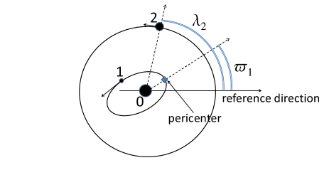
Figure 1: The coplanar triple system composed by two massive black holes (MBHs; 0 and 2) and a compact object (CO; 1). The MBH 0 and the CO 1 form an inner EMRI. We measure the angular position $\varpi_{1}$ of the pericenter of the CO with respect to the fixed reference direction. The outer MBH has a nearly circular orbit and its angular position is given by $\lambda_{2}$. We can similarly define the variable $\lambda_{1}$ for the CO, but it does not appear in our resonant variable $\lambda_{2}-\varpi_{1}\sim const$.

case	$m_{0}$	$m_{1}$	$m_{2}$	$a_{1in}$	$\frac{\alpha}{8}$	$\frac{d\bar{\delta}}{d\tau}$	$D$
I	0.90	0	0.1	50	0.017	0.00168	24.7
II	0.98	0	0.02	30	0.027	0.0289	68.0
III	0.999	0	0.001	20	0.035	1.43	890

Table 1: The model parameters adopted in our numerical simulations. The initial outer semimajor axis $a_{2in}$ is adjusted to yield a resonant encounter. The outer eccentricity is initially set at $e_{2in}\simeq 0$ and it stays at a small value. The left three columns show the basic parameters characterising the resonant dynamics, and they are evaluated for coplanar orbits. The ratio $\alpha/8$ is the critical eccentricity for the shift of the resonant angle $\lambda_{2}-\varpi_{1}$ (discussed in §4). The transverse velocity $d\bar{\delta}/d\tau$ and the coefficient $D$ are defined in §5, and evaluated with respect to the Hamiltonian (49) for the second order resonance.

In Table 1, we present the model parameters of our numerical simulations. Since dependence of the resonant dynamics on the inner eccentricity $e$ is our central issue, we systematically analyze it for commonly arranged sets of parameters such as masses $(m_{0},m_{1},m_{2})$ and the initial inner semimajor axis $a_{1in}$. Among the three models listed in Table 1, we mainly use models I and II, targeting comparable MBHs, and model III is studied for a specific purpose in §4.

In Figs.2-4, we present samples of typical orbital evolutions of model I around the resonant encounters. We set the initial outer distance $a_{2in}$ so that the system transverses the resonant condition due to the radiational orbital decay. Throughout this paper, we use the outer semimajor axis $a_{2}$ to show the time. This variable $a_{2}$ is monotonically decreasing from its initial value $a_{2in}$.

In Fig.2, we show the results from an initial inner eccentricity $e_{in}\simeq 0.1$. The test particle $m_{1}$ is resonantly captured by the outer MBH binary at the time $a_{2}\sim 340$, corresponding to the ratio of orbital periods at $\sim 17$. Incidentally, the inner eccentricity $e$ starts to grow and the inner axis $a_{1}$ decreases very slowly. The resonant variable $\lambda_{2}-\varpi_{1}$ soon localizes around $\sim\pi/2$.

For the run shown in Fig.3, we set a larger initial eccentricity $e_{in}\simeq 0.57$. The test particle $m_{1}$ is captured into the resonance around $a_{2}\sim 280$. In contrast to Fig.2, the combination $\lambda_{2}-\varpi_{1}$ now has a large librational amplitude with a small excluded region around $\pi$. Again, after the resonant capture, the inner eccentricity $e$ increases and the semimajor axis decreases.

In Fig.4, the initial inner eccentricity $e_{in}\sim 0.57$ is close to that in Fig.3. But the initial orbital phases are different between Figs.3 and 4. While evolutions in Figs.3 and 4 are similar down to $a_{2}\sim 280$, their subsequent profiles are completely different. Around the critical epoch $a_{2}\sim 280$, the inner eccentricity $e$ shows a large gap in Fig.4, but the EMRI is not captured into the resonance, as indicated by the rotating variable $\lambda_{2}-\varpi_{1}$. The inner semimajor axis $a_{1}$ also has a small gap, but the following Tisserand relation (Murray & Dermott 2000, but now for a coplanar system) holds nearly smoothly around $a_{2}\sim 280$;

$$\frac{a_{2}}{2a_{1}}+\sqrt{\frac{a_{1}}{a_{2}}(1-e^{2})}\simeq const.$$ (2)

This relation connects the gaps for $e$ and $a_{1}$ in Fig.4.

For the standard MMRs, it is well known that the capture becomes a stochastic process when we increase the eccentricity of the perturbed mass (Borderies & Goldreich, 1984; Peale, 1986; Malhotra, 1988; Dermott, Malhotra, & Murray, 1988; MD, ). In addition, the eccentricity shows a gap if the capture is failed. These interesting characters are successfully explained by the Hamiltonian approach. For our unusual resonance, we make detailed analysis on these issues later in §6 and 7.

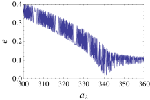
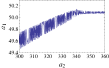
Figure 2: Evolution of a coplanar EMRI-MBH triple system from an inner eccentricity $e\sim 0.1$ (model I). The horizontal axis $a_{2}$ is the semimajor axis of the outer MBH $m_{2}$ and decreases from its initial value $a_{2in}=360$ due to gravitational wave emission. The three panels show the resonant variable $\lambda_{2}-\varpi_{1}$ (the upper left one), the inner eccentricity $e$ (the upper right one, in modulo $2\pi$) and the inner semimajor axis $a_{1}$ (the bottom one). This system encounters the resonance around $a_{2}\simeq 340$, and the capture is successful. The inner eccentricity $e$ starts to increase afterward.

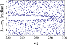
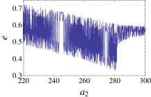
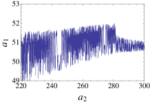
Figure 3: Evolution of a coplanar triple from a large inner eccentricity $e\sim 0.57$ (model I). The inner EMRI is resonantly captured by the outer MBH around $a_{2}\sim 280$. The libration amplitude is large.

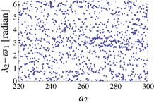
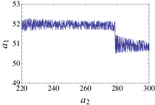
Figure 4: Evolution of a coplanar triple from similar orbital parameters (e.g. $e_{in}\sim 0.57$) as Fig.3 but with a different relative orbital phase (model I). The resonant capture is unsuccessful. We can observe gaps of orbital parameters at the resonant encounter around $a_{2}\sim 280$.

Our main targets in this paper are the EMRI-MBH triple systems in the resonant state $\lambda_{2}-\varpi_{1}\sim const$. But it would be worth mentioning that a related resonant structure was identified in the ring of Saturn (Porco et al., 1984). The Titan ringlet has the semimajor axis of $1.29R_{S}$ ($R_{S}\sim 6\times 10^{4}$km: the radius of Saturn) and is in the resonant state $\lambda_{T}-\varpi_{R}\sim const$ with Titan, the largest satellite of Saturn at the distance $\sim 20R_{S}$. Here $\varpi_{R}$ is the longitude of the pericenter of the ringlet and $\lambda_{T}$ is the mean anomaly of Titan. The apsidal precession $\dot{\varpi}_{R}$ of the ringlet is mainly driven by the multiple moments of Saturn (e.g. its quadrupole moment; $J_{2}=1.6\times 10^{-2}$). This ringlet has a finite eccentricity $e_{R}\sim(2.6\pm 1.4)\times 10^{-4}$ and a radial width $\sim 20$km.

Another potentially interesting example is the Earth-Moon system. In its early history, the system might be resonantly affected by the Sun as an outer perturber, through the state $\lambda_{Sun}-\varpi_{Moon}\sim const$ (Touma & Wisdom, 1998; Ćuk & Stewart, 2012).

3 relativistic apsidal precession

As demonstrated in the previous section, our resonant state is characterized by the following relation between the two angular parameters $\lambda_{2}$ and $\varpi_{1}$

$$\eta\equiv\lambda_{2}-\varpi_{1}\sim const.$$ (3)

Taking the time derivative of this relation, we have

$${n}_{2}\sim\dot{\varpi}_{1}$$ (4)

on average (the dot $\dot{}$ representing the time derivative). Here ${n}_{l}$ is the angular frequency of the object $m_{l}$ ($l=1,2$) around the central MBH $m_{0}$, and evaluated with Kepler’s third law as

$$n_{1} = \left(\frac{m_{0}}{a_{1}^{3}}\right)^{1/2}$$ (5)

$$n_{2} = \left(\frac{m_{0}+m_{2}}{a_{2}^{3}}\right)^{1/2}=m_{0}^{-1/2}n_{1}\left(\frac{a_{1}}{a_{2}}\right)^{3/2}$$ (6)

for $m_{1}\ll m_{0}+m_{2}=1$. To characterize the hierarchy of the inner and outer orbits, we introduce the factor $\alpha$ as

$$\alpha\equiv\frac{a_{1}}{a_{2}}\ll 1.$$ (7)

Then the outer frequency is roughly given as

$$n_{2}\sim n_{1}\alpha^{3/2}$$ (8)

for $m_{0}=O(1)$.

Next we discuss the apsidal precession rate $\dot{\varpi}_{1}$ of the inner EMRI. As is well known for Mercury, relativistic correction generates the precession with the rate

$${\dot{\varpi}}_{1r}=\frac{3m_{0}^{3/2}}{a_{1}^{5/2}(1-e^{2})}=\frac{3pn_{1}}{1-e^{2}}$$ (9)

at the 1PN order (Landau & Lifshitz, 1971). Here, in order to explicitly show the relativistic effects, we additionally defined the post-Newtonian parameter $p$ of the EMRI as

$$p\equiv\frac{m_{0}}{a_{1}}.$$ (10)

In this paper, we only deal with the regime $p\ll 1$ where the PN framework works well. The relativistic precession (9) depends on the eccentricity $e$ as $\propto(1-e^{2})^{-1}$. As we see later in §5, this dependence becomes particularly important for our unusual resonance.

From Eqs.(4)(6) and (9), we obtain the following relation for the onset of the resonance

$$\frac{3p}{1-e^{2}}=m_{0}^{-1/2}\alpha^{3/2}$$ (11)

or equivalently

$$a_{2}=3^{-2/3}a_{1}^{5/3}(1-e^{2})^{2/3}m_{0}^{-1}.$$ (12)

The expression for $e=0$ was studied in the previous paper (Seto 2012, see also Hirata 2011) and we have the relation between the PN parameter $p$ and the orbital hierarchy parameter $\alpha$ as $p\sim\alpha^{3/2}/3$. For the eccentric cases shown in the previous section, Eq.(12) provides $a_{2}\simeq 360$ for Fig.2 and $a_{2}\simeq 285$ for Figs.3 and 4, reasonably reproducing the dependence on the eccentricity $e$.

Eq.(11) is obtained by neglecting influence of the distant outer MBH $m_{2}$ and assuming that the precession rate $\dot{\varpi}_{1}$ is dominated by the relativistic effect $\dot{\varpi}_{1r}$. Here we evaluate the Newtonian secular contribution $\dot{\varpi}_{1N}$ due to $m_{2}$. For moderate eccentricity and inclination, the secular effect $\dot{\varpi}_{1N}$ is estimated as (MD, )

$${\dot{\varpi}}_{1N}=\frac{3}{4}\frac{m_{2}a_{1}^{3/2}}{a_{2}^{3}m_{0}^{1/2}}.$$ (13)

Then, at the critical distance (12), we have

$$\frac{{\dot{\varpi}}_{1N}}{{\dot{\varpi}}_{1r}}=\frac{9}{4}\frac{m_{0}m_{2}}{a_{1}}\ll 1$$ (14)

with $p=m_{0}/a_{1}\ll 1$ and $m_{2}<1$. Therefore, the Newtonian contribution for the precession $\dot{\varpi}_{1}$ would be much smaller than the relativistic one. The distant outer body $m_{2}$ also has a 1PN effect for the precession $\dot{\varpi}_{1}$ (see the 1PN interaction term in Naoz et al. 2012). But its magnitude is $O(\alpha^{2.5})$ times smaller than Eq.(9), and not important for the precession $\dot{\varpi}_{1}$. We hereafter put

$$\dot{\varpi}_{1}=\dot{\varpi}_{1r},$$ (15)

as already assumed to derive Eq.(12).

4 comparison between the first and second order resonances

The gravitational interaction between the inner and outer orbits of a triple system has been perturbatively analyze with the disturbing function (MD, ). For our resonant state $\eta\sim const$ in a coplanar configuration, the relevant element of the disturbing function is expanded as

$$\zeta=e^{1}C_{1,0}\cos\eta+e^{2}C_{2,0}\cos 2\eta,$$ (16)

where we take the terms up to the order $O(e^{2})$. The functions $C_{1,0}$ and $C_{2,0}$ depend on the hierarchy parameter $\alpha\ll 1$ of the orbital configuration. They are explicitly given as

$$C_{1,0}=\frac{2}{3}\alpha-\left(\frac{\alpha\partial_{\alpha}}{2}+1\right)b_{1/2}^{(0)}(\alpha)=-\frac{15}{16}\alpha^{3}$$ (17)

$$C_{2,0}=\left(\frac{3}{4}+\frac{3\alpha\partial_{\alpha}}{4}+\frac{3\alpha^{2}\partial_{\alpha}^{2}}{8}\right)b_{1/2}^{(2)}(\alpha)=\frac{15}{8}\alpha^{2}+\frac{105}{64}\alpha^{4}$$ (18)

with the Laplace coefficients $b_{i}^{(j)}(\alpha)$. In Eq.(17) the first term $2\alpha/3$ is the indirect part and is canceled by the $O(\alpha)$ term of its direct part. As a result, the function $C_{1,0}\propto\alpha^{3}$ has a stronger dependence on the parameter $\alpha(\ll 1)$ than the counterpart $C_{2,0}\propto\alpha^{2}$. Actually, the second-order one $C_{2,0}$ has the lowest power of $\alpha$ among the resonant terms in the form $\cos N\eta$ with $N\geq 1$. We hereafter neglect the term $\propto\alpha^{4}$ in Eq.(18) and put

$$\zeta=-\frac{15}{16}\alpha^{3}e\left(\cos\eta-2\frac{e}{\alpha}\cos 2\eta\right).$$ (19)

This expression shows that the second order term can dominate the first order one even at a small eccentricity $e\sim\alpha$, due to the hierarchy of the system $\alpha\ll 1$.

Interestingly, the competition of the two terms can be directly observed as a shift of the mean angle $\eta$ of libration, during the resonant amplification of the inner eccentricity $e$. We now discuss this in some detail. For simplicity, we assume that the dissipative evolution is negligible during one libration period.

First, the system around the resonance can be effectively reduced to one dimensional system (with the variable $\propto\eta$ and its conjugate momentum $\propto e^{2}$, see §5 for detail). The effective Hamiltonian has the resonant term $\propto\zeta$, and the variable $\eta$ appears only in this term. Then, from the canonical equation, we should have

$$\frac{de^{2}}{dt}\propto\frac{\partial\zeta}{\partial\eta}=0$$ (20)

at the equilibrium point $(e_{e},\eta_{e})$. Thus, for given equilibrium value $e=e_{e}$, we associate the corresponding equilibrium angle $\eta_{e}$ as the minimum of the following potential $V(\propto\zeta)$

$$V\equiv-\cos\eta+\frac{2e_{e}}{\alpha}\cos 2\eta.$$ (21)

The shape of this potential is shown in Fig.5 for representative values of the ratio $e_{e}/\alpha$. The positions of the potential minima qualitatively change at the critical value $e_{e}=\alpha/8$. In Table 1, we present its value for models I-III. At $e_{e}<\alpha/8$, the potential $V$ is dominated by the first order term and we have the equilibrium angle

$$\eta_{e}=0,~{}~{}~{}~{}~{}(e_{e}<\alpha/8).$$ (22)

When increasing $e_{e}$ beyond the critical value $\alpha/8$, the angle $\eta_{e}$ starts to move as

$$\eta_{e}=\pm\arccos(\alpha/8e_{e}),~{}~{}~{}~{}~{}(e_{e}>\alpha/8).$$ (23)

We have $\eta_{e}\simeq\pm\pi/2$ for $e_{e}\gg\alpha/8$, dominated by the second order term in Eq.(21).

Now we examine our simple model (22) and (23) for the equilibrium resonant angle, by using numerical simulations. In Fig.6, we show the evolution of orbital parameters for model III. Owing to its small outer mass $m_{2}$, the forced eccentricity is small at the early stage, and this model allows us to make a suitable demonstration for the present analysis.

The EMRI is resonantly captured by the outer MBH binary around $a_{2}\sim 55$, and its eccentricity $e$ starts to increase afterward. Here the critical eccentricity for the onset of the shift of the equilibrium angle is $\alpha/8\sim 0.035$. Since the libration can be regarded as a circulation around the equilibrium point $(e_{e},\eta_{e})$, the mean value of the libration would be close to the equilibrium point $(e_{e},\eta_{e})$, at least for a small libration amplitude. To directly show the shift of the angle $\eta_{e}$ thorough the resonant amplification of the inner eccentricity $e$, we plot the combination $(e,\eta)$ in Fig.7 together with the analytical model (22) and (23).

Fig.7 shows that, even though the dissipative time scale is not sufficiently long compared with the libration period, the simple analytical prediction shows a good agreement with the numerical one. For a larger libration amplitude as in Fig.3, the potential wall of $V$ around $\eta=0$ (see Fig.5) is easily crossed over, and the angle $\eta$ moves around a broad region, leaving a small excluded regime near $\eta=\pi$.

Note that also in Fig.2, the angle $\eta$ finally localizes around $\pi/2$, as in the case of Fig.6. But this should be regarded as a mere coincidence. Later in §6 and 7, we deal with a large sample of numerical simulations for models I and II. Among them, there are no definite asymmetries for the preference of the two potential minima at $\eta=\pi/2$ and $-\pi/2$ (equivalently $3\pi/2$).

In summary, due to the hierarchy of the orbits with $\alpha\ll 1$, the second order term $\propto e^{2}\alpha^{2}\cos 2\eta$ could become more important than the first order one $\propto e\alpha^{3}\cos\eta$, even for a small eccentricity $e\sim\alpha$. We can observe the resultant shift of the mean (equilibrium) angle $\eta_{e}$ during the resonant amplification of the inner eccentricity $e$.

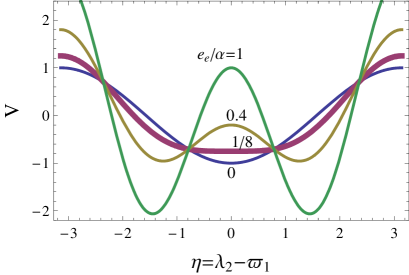
Figure 5: The effective potential $V$ defined in Eq.(21). Its shapes are plotted for representative values of $e_{e}/\alpha$. The equilibrium angle $\eta_{e}$ would be the minimum of the potential. For $e_{e}/\alpha<1/8$, the potential has the single minimum at $\eta=0$, dominated by the first order term. In contrast, for $e_{e}/\alpha>1/8$, we have two minima at $\eta\neq 0$, reflecting the second order component. For larger $e_{e}/\alpha$, the minimal points approach $\pm\pi/2$.

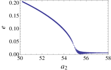
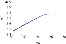
Figure 6: Evolution of the orbital elements of the coplanar inner EMRI for model III. Due to the small outer mass $m_{2}$, the forced components can be suppressed, compared with cases I and II. We have a small initial inner eccentricity $e\sim 0.0065$. The EMRI is captured by the outer MBH binary around $a_{2}\sim 55$. We can clearly observe the shift of the equilibrium angle $\eta_{e}$.

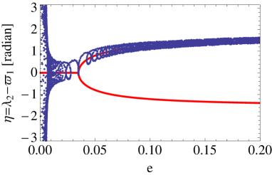
Figure 7: Correspondence between the inner eccentricity $e$ and the resonant angle $\eta=\lambda_{2}-\varpi_{1}$. The points are obtained from the run shown in Fig.6. The red curves are the analytical predictions (22) and (23) for the equilibrium points $(e_{e},\eta_{e})$ with the transition eccentricity at $\alpha/8=0.035$.

5 Hamiltonian Approach

In this section, we apply the Hamiltonian approach for the resonant dynamics of the EMRI-MBH triple systems with $\lambda_{2}-\varpi_{1}\sim const$. By taking appropriate set of conjugate variables, the dynamics around the resonant encounter can be reduced to a simple one dimensional system (Sinclair, 1972; Yoder, 1979; Henrard, 1982; Henrard & Lamaitre, 1983; Peale, 1986; MD, ). For the standard MMRs such as 2:1 or 3:1 resonances, this approach successfully explains characteristic phenomenon around the resonant encounters (Borderies & Goldreich, 1984; Peale, 1986; MD, ). Our aim here is to extend it for our unusual resonance. As detailed descriptions of the approach for the standard MMRs can be found in the literature and many of them are shared with our resonance, it would be unfruitful to lengthily expound all the involved steps. We rather follow the comprehensive formulation given in §8.8 of MD and explain the modifications necessary for our specific resonance.

5.1 Simplified Hamiltonian for Second Order Resonance

Based on the results in the previous section, we analyze the second order resonance with the resonant variable

$$\theta_{1}=j\lambda_{2}+(2-j)\lambda_{1}-2\varpi_{1},$$ (24)

identical to Eq.(8.78) of MD with $k=2$. While we are mainly interested in the specific case $j=2$, we do not fix the parameter $j$ at this stage, in order to enable a simple comparison with the standard second-order MMRs corresponding to $j>2$.

As explained in MD, the variable $\theta_{1}$ has the conjugate momentum $\Theta_{1}$ defined by

$$\Theta_{1} = \frac{m_{1}}{2}\sqrt{m_{0}a_{1}}\left(1-\sqrt{1-e^{2}}\right)$$ (25)

$$\simeq \frac{m_{1}}{4}\sqrt{m_{0}a_{1}}\left(e^{2}+\frac{e^{4}}{4}+\cdots\right).$$ (26)

We should notice that this momentum is directly related to the inner eccentricity $e$ as $\Theta_{1}\propto e^{2}$. In our analytical studies below, we make perturbative expansions, assuming $e\ll 1$.

Among multiple terms in the Hamiltonian (8.98) of MD (denoted as $\cal H$), the key element for our unusual resonance is the following one

$$-k\Theta_{1}{\dot{\varpi}}_{sec}\equiv X$$ (27)

with $k=2$ for the present analysis. Here, the notation $\dot{\varpi}_{sec}$ in MD represents the secular precession rate of the inner pericenter and is identical to the relativistic apsidal precession $\dot{\varpi}_{1r}$ under our prescription in §3 (hereafter using $\dot{\varpi}_{1r}$ in stead of $\dot{\varpi}_{sec}$).

With respect to the canonical equation

$$\frac{d\theta_{1}}{dt}=\frac{\partial{\cal H}}{\partial\Theta_{1}},$$ (28)

the term $X$ in the total Hamiltonian $\cal H$ has a role to provide the secular contribution $-k\dot{\varpi}_{1r}$ for the time derivative $d\theta_{1}/dt$. Therefore, we should have the equation below

$$\frac{\partial X}{\partial\Theta_{1}}=-k{\dot{\varpi}}_{1r}.$$ (29)

Meanwhile, as given in Eq.(9), the relativistic precession rate $\dot{\varpi}_{1r}$ has the following form at 1PN order

$${\dot{\varpi}}_{1r}=\frac{3pn_{1}}{1-e^{2}}\simeq 3pn_{1}(1+e^{2}),$$ (30)

and the rate ${\dot{\varpi}}_{1r}$ itself depends on the conjugate momentum $\Theta_{1}\propto e^{2}$. Thus we have the following perturbative solution $X$ for Eq.(29)

$$X = -3kpn_{1}\Theta_{1}\left(1+\frac{e^{2}}{2}\right)$$ (31)

$$= -3kpn_{1}\Theta_{1}\left(1+\frac{2\Theta_{1}}{m_{1}\sqrt{m_{0}a_{1}}}\right)$$ (32)

expanded in terms of the momentum $\Theta$, instead of the eccentricity $e$. Note that this solution is different from the naive expression (27) that is perturbatively expanded as

$$-k\Theta_{1}{\dot{\varpi}}_{sec}=-3kpn_{1}\Theta_{1}\left(1+\frac{4\Theta_{1}}{m_{1}\sqrt{m_{0}a_{1}}}\right).$$ (33)

The quadratic term $\propto\Theta_{1}^{2}$ plays a critical role for our resonance, as we see in the next subsection. This term originates from the dependence $\dot{\varpi}_{1r}\propto(1-e^{2})^{-1}$.

One might has an impression that the present derivation for Eq.(32) is phenomenological, as it is constructed to reproduce the desired precession rate $\dot{\varpi}_{1r}$. But we can actually derive the term (proportional to $e^{2}+3e^{4}/4+\cdots$) identical to $X$ in Eq.(32), starting directly from the 1PN Hamiltonian $H_{1}$ in Eq.(1) (see Eq.(28) in Naoz et al. 2012). We took the above route to elucidate the modification relative to the typical analysis for the standard MMRs.

With the explicit form of the relativistic correction $X$ in hand, we can next apply the standard arguments in MD to derive a simplified Hamiltonian for MMRs. After some calculations (e.g. introducing the new conjugate variables $\theta_{1}^{\prime}=\theta_{1}/2$ and $\Gamma\equiv 2\Theta_{1}$), we have the following Hamiltonian (corresponding to Eq.(8.102) of MD)

$${\cal H}^{\dagger}={\bar{\alpha}}\Gamma+{\bar{\beta}}\Gamma^{2}+2{\bar{\epsilon}}\Gamma\cos 2\theta_{1}^{\prime}.$$ (34)

Here the coefficients $\bar{\alpha},\bar{\beta}$ and $\bar{\epsilon}$ are given as

$${\bar{\alpha}}=\frac{(j-2)n_{1}-jn_{2}+6pn_{1}}{2},$$ (35)

$${\bar{\beta}}=\frac{3}{8}\left(\frac{(j-2)^{2}}{m_{1}a_{1}^{2}}+\frac{j^{2}}{m_{2}a_{2}^{2}}\right)+3\frac{p}{m_{1}a_{1}^{2}},$$ (36)

$$\bar{\epsilon}=C_{j,j-2}n_{1}\frac{m_{2}}{m_{0}}\alpha.$$ (37)

In Eqs.(35) and (36), the terms proportional to the PN parameter $p$ clearly show the relativistic corrections. The factor $C_{j,j-2}=C_{2,0}$ for $j=2$ was already given in Eq.(18). In the right-hand side of Eq.(36), the first parenthesis appears in the standard MMRs and has its origin in the Keplarian terms in the triple system (see MD). Its second term ($\propto p$) is due to the quadratic term $\propto\Theta_{1}^{2}$ in the secular correction $X$ for the relativistic apsidal precession.

We further make transformation of variables as follows

$$\Phi=\frac{\Gamma\bar{\beta}}{2\bar{\epsilon}}=\frac{\Theta_{1}\bar{\beta}}{\bar{\epsilon}},~{}~{}\tau={2\bar{\epsilon}}{t}$$ (38)

$$\phi=\cases{\theta_{1}^{\prime}&(${\bar{\epsilon}}<0$)\cr\theta_{1}^{\prime}+\pi&(${\bar{\epsilon}}>0$)\cr},$$ (39)

and finally obtain the rescaled Hamiltonian

$$H=\Phi^{2}+\bar{\delta}~{}\Phi+\Phi\cos 2\phi$$ (40)

with the single parameter $\bar{\delta}$ defined by

$$\bar{\delta}=\frac{\bar{\alpha}}{2\bar{\epsilon}}.$$ (41)

The associated canonical equations are written as

$$\frac{d\Phi}{d\tau}=-\frac{\partial H}{\partial\phi},~{}~{}\frac{d\phi}{d\tau}=\frac{\partial H}{\partial\Phi}.$$ (42)

The rescaled Hamiltonian (40) is slightly different from the related expression (8.116) in MD, but identical to those in Quillen (2006) and Mustill & Wyatt (2011). We adopt the present form, in order to use these two references later and discuss whether evolution of the parameter $\bar{\delta}$ can be regarded as adiabatic for our resonant dynamics.

Roughly speaking, this parameter $\bar{\delta}$ represents an effective distance to the resonance. Due to the GW emission, the orbits of the EMRI-MBH triple system decay gradually, and the parameter $\bar{\delta}$ varies accordingly.

We now estimate the transition rate $d\bar{\delta}/d\tau$. First, apart shortly from the triple systems, we consider a simple binary with a semimajor axis $a$, an eccentricity $e$ and masses $m,m^{\prime}$. Its orbital decay rate $da/dt$ by GW emission is given as (Peters, 1964)

$$\frac{da}{dt}=-\frac{64}{5}\frac{mm^{\prime}(m+m^{\prime})}{a^{3}(1-e^{2})^{7/2}}\left(1+\frac{73}{24}e^{2}+\frac{37}{96}e^{4}\right).$$ (43)

Next, for our triples, we assume that, before the resonant encounters, the EMRI and MBH binary independently evolve with Eq.(43). Then we obtain

$$\frac{d\bar{\alpha}}{dt} = \frac{48}{5}\Big{[}m_{1}m_{0}^{5/2}a_{1}^{-13/2}\frac{\left\{(j-2)a_{1}+10m_{0}\right\}}{(1-e^{2})^{7/2}}$$ (44)

$$\times\left(1+\frac{73}{24}e^{2}+\frac{37}{96}e^{4}\right)-jm_{0}m_{2}a_{2}^{-11/2}\Big{]}$$

for $e_{2}=0$. With the scaled time $\tau$, we can obtain the transition rate as

$$\frac{d\bar{\delta}}{d\tau}=\frac{1}{2\bar{\epsilon}}\frac{d\bar{\alpha}}{dt}\frac{dt}{d\tau}=\frac{1}{4\bar{\epsilon}^{2}}\frac{d\bar{\alpha}}{dt}.$$ (45)

For a given EMRI-MBH triple around the resonant encounter, we can now analyze its evolution through the one-dimensional rescaled Hamiltonian (40). The information of the original triple system is converted to (i) the new variables $(\phi,\Phi)$, (ii) the parameter $\bar{\delta}$ and (iii) its time derivative $d\bar{\delta}/d\tau$. In practice, this mapping can be made with Eqs.(35)-(39) and (44)-(45). In the next subsection, we concretely study the relation in the test particle limit $m_{1}\to 0$. But, here, we derive a result valid also for $m_{1}\neq 0$.

To realize a capture (i.e. transition of $\phi$ from rotation to libration) with Eq.(42), the resonance should be crossed in the direction $d\bar{\delta}/d\tau<0$ (Peal 1986; MD). In the cases of standard MMRs, this corresponds to relatively approaching orbits. For example, to be captured into the 3:2 resonance, the ratio of the orbital periods should change in the direction of $1.6\to 1.5$ not $1.4\to 1.5$. With Eqs.(12) and (44) for $j=2$, the inequality $d\bar{\delta}/d\tau<0$ is rewritten as

$$\frac{a_{1}}{a_{2}}>\sqrt{\frac{5}{3}(1-e^{2})^{-5/2}\left(1+\frac{73}{24}e^{2}+\frac{37}{96}e^{4}\right)\left(\frac{m_{0}m_{1}}{m_{2}}\right)^{1/2}}.$$ (46)

For the specific case $e=0$, this expression agrees with that derived and examined in Seto (2012). Note that our labels $(0,1,2)$ for the three masses are different from those in Seto (2012).

5.2 Test Particle Limit

Here we discuss the mapping between the EMRI-MBH triple system and the simplified Hamiltonian system (40) in the test particle limit $m_{1}\to 0$. In this limit, we can easily control the relative orbital evolutions of the triple system in numerical simulations, and, furthermore, the role of the post-Newtonian corrections becomes transparent.

From Eqs.(26)(36)(37) and (38), the inner eccentricity $e$ is related to the momentum $\Phi$ as

$$\Phi=\frac{m_{0}a_{1}^{2}}{20m_{2}\alpha^{3}}\left[\frac{(j-2)^{2}}{a_{1}^{2}}+\frac{m_{1}j^{2}}{m_{2}a_{2}^{2}}+\frac{8p}{a_{1}^{2}}\right]e^{2}.$$ (47)

In this relation, we pay our attention to the dependence of the mass parameter $m_{1}$. We can put $p=0$ in the traditional analysis of the standard MMRs with $j>2$ (see Eq.(8.109) of MD). However, for our unusual one with $j=2$, the mapping (47) becomes singular $\Phi\propto m_{1}e^{2}$ in the limit $m_{1}\to 0$, if the relativistic effect is dropped with $p=0$. Therefore, interestingly, the regularity of the mapping (47) is maintained by the post-Newtonian correction ($\propto p$) for our resonance with $j=2$ as

$$\Phi=\frac{2pm_{0}a_{2}^{3}e^{2}}{5m_{2}a_{1}^{3}}$$ (48)

without depending on $m_{1}$. As mentioned earlier, the post-Newtonian term in Eq.(47) comes from the quadratic term of the momentum $\Phi$ in Eq.(32) and intrinsically from the dependence of the precession rate on the eccentricity as shown in Eq.(9).

Now we derive formulae specifically for $j=2$ with the rescaled Hamiltonian

$$H=\Phi^{2}+\bar{\delta}~{}\Phi+\Phi\cos 2\phi.$$ (49)

The variable $\phi$ is related to the original resonant angle $\eta\equiv\lambda_{2}-\varpi_{2}$ as

$$\phi=\eta+\pi.$$ (50)

After some algebra with Eq.(12), the principal quantities for the rescaled Hamiltonian are given by the original parameters as

$$\Phi=De^{2}$$ (51)

$$D\equiv\frac{2a_{1}}{45m_{0}m_{2}}$$ (52)

$$\frac{d\bar{\delta}}{d\tau}=-\frac{512m_{0}^{3/2}}{3^{1/3}375m_{2}a_{1}^{13/6}}.$$ (53)

Note that the transit speed $d\bar{\delta}/d\tau$ is nearly constant around the resonant encounter, and we omit the expression for the time dependent parameter $\bar{\delta}$ itself.

In Table.1, we provide the transit speed $d\bar{\delta}/d\tau$ as well as the coefficient $D$. The former is an useful measure to discuss the adiabaticity of the time evolution of the parameter $\bar{\delta}$ at the resonant encounter.

For comparison, including only the first order resonant term $\propto e$ in Eq.(19), we derive the relevant expressions for the test particle limit. In Appendix A, we summarize the results. Again, we have a regular mapping between the momentum $\Phi$ and the inner eccentricity $e$, due to the PN correction.

For a Newtonian apsidal precession induced by multiple moments of masses, the precession rate at $e\ll 1$ generally has correction for the eccentricity $e$ starting from $e^{2}$ (Sterne, 1939). Therefore, the mapping to a corresponding rescaled Hamiltonian becomes regular, as for the relativistic one discussed above. For example, the precession rate of a test particle due to the quadrupole moment $J_{2}$ of the central body is expanded as $\dot{\varpi}\propto J_{2}(1+2e^{2}+\cdots)$.

In the next three sections, using the mapping from the EMRI-MBH triple system, we make quantitative predictions on the resonant dynamics and compare them with numerical simulations. Below, we limit our analysis to the test particle limit $m_{1}\to 0$.

6 capture rate

In this section, we study whether the analytical model based on the rescaled Hamiltonian can reproduce the capture rate estimated from numerical simulations.

For this comparison, we obtained the capture rate from the numerical side in the following manner. First, for models I and II, we took various ($\sim 13$) inner initial eccentricities $e_{in}$ between $\sim 0$ and $\sim 0.7$. For each eccentricity, we assigned an initial outer radius $a_{2in}$ larger than Eq.(12) to assure a resonant encounter, and made 20 runs starting from randomly distributed relative orbital phases. Therefore, the total number of the runs is $\sim 2\times 13\times 20\sim 500$. We judge a run as a resonantly captured event when the angle $\eta=\lambda_{2}-\varpi_{1}$ has a single excluded range $\Delta\eta$ larger than $\pi/10$ for minimum duration $a_{2}/10$ (and also $a_{2}/20$ for comparison) in terms of the decaying outer radius $a_{2}$ (see e.g. Figs.2 and 3). An MMR is often identified with a sharp concentration of a resonance angle, as found in Fig.2. But, here, we employed the criteria for $\Delta\eta$ to handle the resonant state with large libration amplitudes, as demonstrated in Fig.3.

Then, for each initial eccentricity $e_{in}$, we counted the number of captured events among the associated 20 runs and roughly obtained the capture rate. We provide the numerical results in Fig.8 with the blue circles for minimum duration $a_{2}/10$. Up to moderate eccentricity, we obtain the same results for the minimum duration $a_{2}/20$. Only when they are different, we added the latter with the open squares. . As shown in Figs.2-4, the eccentricities of the EMRIs are always oscillating to some extent. To handle this, we took time averaged eccentricity for each run at its early stage, and subsequently evaluated the mean value among the 20 runs. The initial eccentricities in Fig.8 are made up in this way.

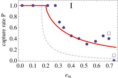
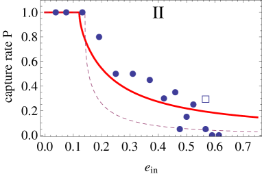
Figure 8: Resonant capture rate of an inner EMRI by a coplanar outer MBH. The results are given as functions of the inner eccentricity $e_{in}$ for models I and II. The solid curves are the analytical predictions $P_{2}$ for the second order term $\propto\cos 2\eta$ and the dashed curves are $P_{1}$ for the first-order term $\propto\cos\eta$. The circles are numerical results for minimum duration $a_{2}/10$, and the additional open squares are for $a_{2}/20$ (shown only if different). Each of them is estimated from 20 runs.

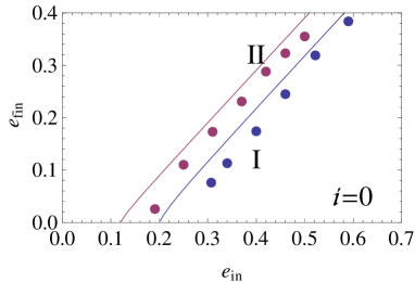
Figure 9: Gaps of the eccentricities $e$ of inner EMRIs with failed captures (as shown in Fig.4). With the solid curves, we plot the analytic correspondences between the gapped eccentricities before ($e_{in}$) and after ($e_{fin}$) the resonant encounter for models I and II. The circles are the mean eccentricities of the numerical runs accompanied by the gaps.

Next we analytically estimate the capture rate through the rescaled Hamiltonian (49), following Borderies & Goldreich (1984). In Appendix B, we briefly describe their results. As we have already discussed, the second order resonance is relevant for our systems (unless $e_{in}$ is less than $O(10^{-2})$, see Table 1). Therefore, we mainly use their results for $k=2$ (see §B1).

For an initial eccentricity $e_{in}$, the analytical rate $P_{2}$ is obtained through the projected initial momentum

$$\Phi_{in}=De_{in}^{2}$$ (54)

for the rescaled Hamiltonian. There is a critical value $\Phi_{cr}=1$, corresponding to $e_{in}=\sqrt{\Phi_{cr}/D}=0.20$ (model I) and 0.12 (model II) that are much larger than $\alpha/8=O(10^{-2})$ (see Table 1). The capture occurs at 100% for $\Phi_{in}<\Phi_{cr}$. Meanwhile, for $\Phi_{in}>\Phi_{cr}$, the capture becomes a stochastic process with the rate $P_{2}$ defined implicitly by Eqs.(66) and (67).

In Fig.8, with the solid curves, we present the analytical rates $P_{2}$. At $e_{in}\la 0.4$, they show reasonable agreements with the numerical ones. But, at larger eccentricities $e_{in}\ga 0.5$, we have significant discrepancies. This is not surprising, since we made, at least, various approximations, valid only for $e_{in}^{2}\ll 1$. For reference, we also show the rate $P_{1}$ expected for the fist order resonance (see §B.2), but it poorly fits the numerical data, as expected. Note also that, for higher eccentricities, the numerical results are affected by the applied conditions for identification of the resonances.

As we explained earlier, the critical eccentricity $\sqrt{\Phi_{cr}/D}$ characterises the overall shape of the capture rate. Here we should comment on its magnitude for the standard second-order MMRs (with the variable (24) at $j>2$). For these resonances, dynamical stability of orbits requires $m_{2}\ll m_{0}$ (assuming $m_{1}<m_{2}$). Then we can show a scaling behaviour $D=\Phi/e^{2}\propto 1/m_{2}$ and obtain the critical eccentricity $\sqrt{\Phi_{cr}/D}\ll 1$ much smaller than our hierarchical one with $m_{0}/m_{2}=O(1)$ (as in model I). Therefore, for the standard second-order MMRs, perturbative expansion of the eccentricity is more effective in the regime where the resonant capture is probable (e.g. $P_{2}>0.1$), unlike our hierarchical one with larger $\sqrt{\Phi_{cr}/D}$. We can make similar arguments for the first-order resonances.

For the analytical predictions in Appendix B, we fully use the arguments based on the adiabatic invariant that is conserved for a transit speed $|d\bar{\delta}/d\tau|$ much smaller than the libration frequency (Landau & Lifshitz, 1969). To examine the impacts of finiteness of $|d\bar{\delta}/d\tau|$ on the resonant dynamics, Quillen (2006) and Mustill & Wyatt (2011) numerically studied dependence of the capture rate on the transition speed $|d\bar{\delta}/d\tau|$. Their results (see e.g. Fig.2 in Mustill & Wyatt 2011) indicate that the adiabatic approximation would be efficient for $|d\bar{\delta}/d\tau|<0.1$. As shown in Table.1, two models I and II well satisfy this criteria. For a coplanar EMRI-MBH triple of comparable MBHs ($m_{2}/m_{0}=O(1)$) with converging orbits $d\bar{\delta}/d\tau<0$, we generally have $|d\bar{\delta}/d\tau|\ll 0.1$, unless the target EMRI is highly relativistic.

7 gap of inner eccentricity

It is well known that, for the standard MMRs, the eccentricity of a perturbed body shows a gap when the resonance is encountered but capture results in failure (e.g. Peale 1986; MD; see also Amaro-Seoane et al. 2012). This phenomena is well explained by the Hamiltonian approach in the associated phase space, as a rapid change of rotational motion at the separatrix crossing. In Fig.4, we can observe a similar gap of the eccentricity for the run without a resonant capture.

In order to further examine validity of our Hamiltonian model extended for the unusual resonance, we analyze the correspondence of the two eccentricities; $e_{in}$ (before the encounter) and $e_{fin}$ (after the encounter). We derive an analytical prediction using the rescaled second-order Hamiltonian (49) and compare it with the numerical simulations done in §6.

We first discuss the analytical approach in which the correspondence between the two eccentricities is equivalent to the relation between the initial momentum $\Phi_{in}=De_{in}^{2}$ and the final one $\Phi_{fin}=De_{fin}^{2}$ both far from the resonant encounter. For a given initial momentum $\Phi_{in}$, the parameter $\bar{\delta}$ at the separatrix crossing is given in a somewhat complicated form as in Eqs.(67) and (68). But, because of a simple expression for a define integral, we have the following concise relation between the two momenta (Malhotra, 1988)

$$\Phi_{in}+\Phi_{fin}=-\bar{\delta}.$$ (55)

Note that the separatrix relevant for our analysis is formed at $\bar{\delta}<-1$ where the capture rate becomes less than unity. In Eq.(55), we have $\Phi_{in}=1$ and $\Phi_{fin}=0$ for $\bar{\delta}=-1$.

We can now obtain the desired correspondence $\Phi_{in}\to\Phi_{fin}$ (equivalently $e_{in}\to e_{fin}$) through the intervening parameter $\bar{\delta}(<-1)$. In Fig.9, we show this analytical correspondence for models I and II with the solid curves.

We also analyze the samples of the numerical simulations described in the previous section. In Fig.9, the numerical results are presented with the filled circles. In numerical data, formation of a gap can be easily identified as a instantaneous event, compared with continuation of a resonant state. We can observe small systematic deviations between the analytical and numerical results. But, as a whole, the simple analytical predictions show reasonable agreements with the numerical ones that were obtained after rather complicated dynamical evolutions.

8 inclined orbits

So far we have discussed the resonant dynamics for coplanar orbits. In this section, we extend our study to inclined orbits. We use the parameter $i$ as the relative inclination angle between the inner and outer orbits.

In Fig.10 we provide a numerical example for inclined orbital configurations. This triple system has a small initial inclination angle $i=5.8^{\circ}$, but its initial semimajor axes $a_{1}$, $a_{2}$ and eccentricity $e$ are close to those in Fig.2. We find that the overall evolution of the three quantities $\lambda_{2}-\varpi_{1}$, $e$ and $a_{1}$ are similar to Fig.2.

Note that the inclination angle $i$ stays nearly at a constant value. This is in accord with the simplified Hamiltonian approach that has only two dynamically important variables $e$ and $\lambda_{2}-\varpi_{1}$ in the present eccentricity resonance.

In Fig.11, we show the results from a larger inclination angle $i=60^{\circ}$. In the lower right panel, evolution of the inclination angle $i$ is presented in a geometric form $\cos i$. We can observe oscillation of $\cos i$. But, around the resonant encounter $a_{2}\sim 305$, its amplitude is much smaller than that of the eccentricity $e$.

Figure 10: Evolution of an EMRI-MBH triple system from an inner eccentricity $e=0.10$ (model I). This system has initial parameters similar to Fig.2, but with an initial relative inclination $i\sim 5.8^{\circ}$. The EMRI is captured into resonance around $a_{2}\simeq 340$. The inclination angle $i$ is within $5.7^{\circ}<i<6.0^{\circ}$.

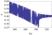
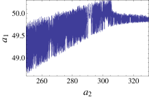
Figure 11: Evolution of an EMRI-MBH triple system from an inner eccentricity $e\sim 0.39$ and relative inclination $i\sim 60^{\circ}$ (model I). This system encounters the resonance around $a_{2}\simeq 305$ where the inner eccentricity $e$ shows larger variation $\Delta e\sim 0.2$ compared with $\Delta\cos i\sim 0.03$.

In the analytical Hamiltonian approach, we need to clarify how the resonant interaction depends on the inclination angle. Here, based on the above numerical demonstrations, we make an approximation that the inclination angle $i$ is constant around the resonant encounter. In the previous case for coplanar orbits, the disturbing function has the following second-order resonance term

$$\zeta=\frac{15\alpha^{2}e^{2}}{8}\cos 2\eta.$$ (56)

Here we neglected subleading contributions of $o(\alpha^{2}e^{2})$. In celestial mechanics, the effects of the inclination on the disturbing function are often handled perturbatively with the expansion parameter $s\equiv\sin[i/2]$. But, here, we are interested in highly inclined orbits with $s=O(1)$, well beyond the perturbative regime $s\ll 1$.

We should notice that the factor ${\bar{\epsilon}}$ for the resonant term in the Hamiltonian (34) is contributed by all the terms proportional to $\cos 2\eta$ among the disturbing function. Fortunately, we can readily collect the terms at the lowest order $\alpha^{2}e^{2}\cos 2\eta$ as follows;

$$\zeta = \frac{15\alpha^{2}e^{2}}{8}(1-2s^{2}+s^{4})\cos 2\eta$$ (57)

$$= \frac{15\alpha^{2}e^{2}}{8}\cos^{4}[i/2]\cos 2\eta.$$ (58)

Therefore, with respect to the original Hamiltonian ${\cal H}^{\dagger}$ given in Eq.(34) and at the order $O(\alpha^{2}e^{2})$ of the resonant interaction, we just need to multiply the factor $\cos^{4}(i/2)$ to the parameter $\bar{\epsilon}$ that was defined in Eq.(37) for the coplanar system. Under the present approximation $i=const$, this is basically what we need to do for dealing with the inclined orbits. Accordingly, for the rescaled Hamiltonian (49) in the test particle limit (see §5.2), the coefficients $D$ in Eq.(52) and the transition speed $d\bar{\delta}/d\tau$ are given as

$$D=\frac{2a_{1}}{45m_{0}m_{2}\cos^{4}[i/2]},$$ (59)

$$\frac{d\bar{\delta}}{d\tau}=\frac{512m_{9}^{3/2}}{3^{1/3}375m_{2}a_{1}^{13/6}\cos^{8}[i/2]}.$$ (60)

With these expressions, it is straightforward to apply the previous analytical methods in §6 and 7 to inclined orbits.

Now, we compare these analytical predictions with numerical simulations for triple systems. Below, we fix the inclination angle at a relatively large value $i=60^{\circ}$ and performed a large number of simulations for two models I and II. Even with the strong dependence on the inclination $\propto 1/\cos^{8}[i/2]=(4/3)^{4}=3.2$, the transition speeds $d\bar{\delta}/d\tau$ are less than 0.1 both with models I and II (see Table 1), and the adiabatic approximation would be still effective for analyzing resonant dynamics.

Note also that due to the relativistic apsidal precession, the Kozai process (Kozai, 1962; Lidov, 1962) does not work here (Holman, Touma, & Tremaine, 1997; Blaes, Lee, & Socrates, 2002; Seto, 2012). Even for $m_{2}\sim m_{1}$, the characteristic frequency of Kozai process is $O(\alpha^{3}n_{1})$, while the 1PN precession frequency of the inner EMRI is $\sim 3pn_{1}$. When a system encounters our resonance, we have $\alpha^{3/2}=3p\ll 1$ (see Eq.(11)) and the Kozai process is suppressed by the 1PN precession effect (see also Naoz et al. 2012). Note that the semi major axes of the systems shown here are not constant of motion, and the orbital averaging associate with the Kozai mechanism cannot be applied here. These systems lay below the stability criterion presented in Lithwick & Naoz 2011.

As for the coplanar orbits, we present the capture rates (Fig.12) and the gaps of the eccentricities (Fig.13). The analytical predictions based on the Hamiltonian approach show good agreements with the numerical results at $e\la 0.4$.

The favourable results in this section could be regarded as additional supports for validity of our Hamiltonian approach extended for the relativistic resonance.

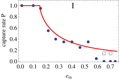
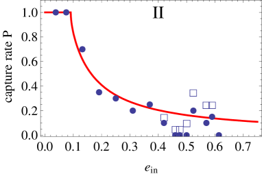
Figure 12: Resonant capture rate of an inner EMRI with the inclination angle $i=60^{\circ}$. The solid curves are given by the Hamiltonian approach with the second order mode. The circles are results from numerical results (each from 20 runs) with the minimum duration $a_{2}/10$ of the resonant state, and the additional open squares are for $a_{2}/20$ (shown only if different).

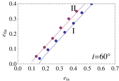
Figure 13: Correspondences of the eccentricities around the resonant encounters. The results are given for models I and II, as in Fig.8, but now for inclined orbits with $i=60^{\circ}$.

9 Summary

We have studied dynamics of the resonant state $\lambda_{2}-\varpi_{1}\sim const$ for a triple system composed by an EMRI (CO+MBH) and an additional outer MBH. This resonant state is supported by the relativistic apsidal precession of the inner EMRI, and does no depend on its mean anomaly $\lambda_{1}$. As a result, the two orbits can become hierarchical with $\alpha\equiv a_{1}/a_{2}\ll 1$, and then the two masses of the MBHs $m_{0}$ and $m_{2}$ can become comparable, in contrast to the standard MMRs where we have $m_{1},m_{2}\ll m_{0}$ due to dynamical stability of orbits with $\alpha=O(1)$.

As a preliminary analysis, in §4, we discussed the dominant order of the resonant interaction for our state $\lambda_{2}-\varpi_{1}\sim const$. Due to the orbital hierarchy, dependencies on the parameter $\alpha(\ll 1)$ play a critical role to assess the relevant terms, and the second-order one $\propto\alpha^{2}e^{2}$ ($e$: the eccentricity of the EMRI) could become more important than the first-order one $\propto e\alpha^{3}$. This result is remarkably different from the standard MMRs for which the parameter $\alpha=O(1)$ is less important.

In §5, we derive the mapping from the resonant triple systems to the rescaled one-dimensional Hamiltonian for the state $\lambda_{2}-\varpi_{1}\sim const$. We basically followed the framework of the Hamiltonian approach explained in the literature, but payed special attention to the term associated with the relativistic apsidal precession $\dot{\varpi}_{1r}$. Here the dependence $\dot{\varpi}_{1r}\propto(1-e^{2})^{-1}$ on the eccentricity $e$ is the key element for the structure of the derived Hamiltonian. The mapping from the original EMRI-MBH triple system to the rescaled Hamiltonian becomes regular even with the test particle limit $m_{1}\to 0$ where the difference from the standard MMRs would become clear.

Then, based on the derived mapping, we made analytical predictions on the dynamical evolution of the state $\lambda_{2}-\varpi_{1}\sim const$ around the resonant encounter and compare them with numerical simulations.

In §6, we studied the resonant capture rate as a function of the eccentricity $e$. For the analytical rate, we incorporated the mapping derived in §5 with the expressions given by Borderies & Goldreich (1984) for the rescaled Hamiltonian. We found that our analytical rates show reasonable agreements with numerical results for eccentricity $e\la 0.4$ where we can perturbatively deal with the effects of the eccentricity $e$.

In §7, we studied the gap of the inner eccentricity when the capture is failed. With the rescaled Hamiltonian, this characteristic phenomena can be understood as a sudden change of periodic motion at a separatrix crossing. We showed that our analytical predictions matches numerical results well.

Finally, in §8, we discussed relatively inclined orbits. By evaluating dependence of the disturbing function on the inclination angle, we can derive the relevant expressions required for the mapping between the inclined triple system to the rescaled Hamiltonian. Again, our analytical prediction reproduces numerical results well for $e\la 0.4$.

In this paper, setting EMRI-MBH triple systems as our concrete astrophysical targets, we studied the hierarchical resonant state $\lambda_{2}-\varpi_{1}\sim const$ induced by relativistic apsidal precession. Similar analyses might be useful for purely Newtonian systems such as a planet orbiting around one component of binary stars. Also in these cases, the mapping could be well behaved in the test particle limit $m_{1}\to 0$, due to preferred dependencies of the apsidal precession rates on the inner eccentricities.

This work was supported by JSPS (20740151, 24540269) and MEXT (24103006).

Appendix A First Order Resonance

In Eq.(19) we expand the resonant potential $\zeta$ up to second-order in eccentricity $e$. In §5, we derive the mapping to the simplified Hamiltonian only including the second order mode $e^{2}\cos 2\eta$. Here we present formulae keeping the first-order mode $\propto e\cos\eta$ alone in the test particle limit $m_{1}\to 0$. The basic procedure is the essentially the same as §5. After some algebra, the rescaled Hamiltonian is given in the forms

$$H=\Phi^{2}+\bar{\delta}\Phi-\Phi^{1/2}\cos(\phi)$$ (61)

with $\phi\equiv\eta$. The momentum $\Phi$ is related to eccentricity as

$$\Phi=Ee^{2}$$ (62)

with the coefficient

$$E\equiv\frac{2^{4/3}a_{1}^{10/9}}{3^{16/9}5^{2/3}m_{2}^{2/3}m_{0}^{4/3}}.$$ (63)

Meanwhile the transition speed $d\bar{\delta}/d\tau$ is expressed with the original parameters of the triple system as

$$\frac{d\bar{\delta}}{d\tau}=-\frac{2^{29/3}m_{0}^{5/6}}{3^{8/9}5^{7/3}a_{1}^{35/18}m_{2}^{1/3}}.$$ (64)

Note that Eqs.(63) and (64) are regular in the test particle limit, as in the case for the second-order mode.

Appendix B analytical formulae for the resonant capture rates

Borderies & Goldreich (1984) analytically evaluated the resonant capture rate for a simplified Hamiltonian

$$H^{\prime}=\Phi^{2}+\bar{\delta}~{}\Phi+(-1)^{k}\Phi^{k/2}\cos k\phi$$ (65)

with $k=1$ (first-order resonance) and $k=2$ (second-order resonance). Here a capture means that the motion of the angle $\phi$ shifts from a rotation in the full angular range $[0,2\pi]$ to a libration within a limited range. We should note that, as partially demonstrated in §5, perturbative expansion for the eccentricity $e$ is crucial to derive the rather simple forms (65).

The goal in this appendix is to provide their capture rates as functions of the initial momentum $\Phi_{in}$. We do not intend to fully explain the arguments in Borderies & Goldreich (1984), but concisely presents their main results. We basically deal with the two cases $k=2$ and $k=1$ separately in §B1 and B2 below. Before going into analyses specific to each mode, we firstly describe the features common to $k=2$ and 1. Here we omit the label $k$, if unnecessary

We consider a case when the parameter $\bar{\delta}$ decreases adiabatically from $\bar{\delta}\gg 1$ down to $\bar{\delta}\ll-1$. At an initial epoch $\bar{\delta}_{in}\gg 1$, far from resonance, the structure of a curve $H^{\prime}=const$ is simple. We have $\Phi\simeq\Phi_{in}=const$ with the conjugate variable $\phi$ rotating in the full range $[0,2\pi]$. When the parameter $\bar{\delta}$ becomes less than a critical value $\bar{\delta}_{cr}$ (depending on the parameter $k$), the Hamiltonian $H^{\prime}$ now has an inner separatrix, in addition to an outer one. We denote the areas inside these two separatrixes by $2\pi\Phi_{I}$ (inner) and $2\pi\Phi_{O}$ (outer), as functions of the epoch $\bar{\delta}$. For the critical value $\bar{\delta}=\bar{\delta}_{cr}$, we put $\Phi_{cr}\equiv\Phi_{O}(\bar{\delta}_{cr})$ (with the identity $\Phi_{I}(\bar{\delta}_{cr})=0$).

From conservation of an adiabatic invariant (Landau & Lifshitz, 1969), the system with an initial value $\Phi_{in}<\Phi_{cr}$ is captured into the resonance at $100\%$, namely with the capture rate of $P(\Phi_{in})=1$. In terms of the decreasing parameter $\bar{\delta}$, this happens at $\bar{\delta}>\bar{\delta}_{cr}$.

But, for $\Phi_{in}\geq\Phi_{cr}$, the resonant encounter occurs at $\bar{\delta}\leq\bar{\delta}_{cr}$ with the capture rate $P_{k}(\Phi_{in})<1$ that was estimated using an argument based on energy balance (see e.g. Goldreich & Peale 1966). If the capture failed, the system starts to rotate near the inner separatrix and soon relaxes to a simple rotation state with the magnitude $\Phi=\Phi_{I}$ ($\Phi_{I}$: evaluated at the resonant encounter).

Below, for $k=1$ and 2, we separately provide the formulae that were given in Borderies & Goldreich (1984) but appropriately adjusted for the specific forms of our Hamiltonian (65).

B.1 Second-Order Resonances; $k=2$

The critical values are $\bar{\delta}_{cr}=-1$ and $\Phi_{cr}=1$. The capture rate for $\Phi_{in}>\Phi_{cr}$ is

$$P_{2}(\Phi_{in})=\frac{2}{1+\frac{\pi}{2\arcsin[(-\bar{\delta})^{-1/2}]}},$$ (66)

where the parameter $\bar{\delta}$ is related to $\Phi_{in}$ as

$$\Phi_{in}=\Phi_{O}(\bar{\delta})$$ (67)

with the explicit form $\Phi_{O}(\bar{\delta})$ as

$$\Phi_{O}(\bar{\delta})=\frac{(-\bar{\delta}-1)^{1/2}}{\pi}-\frac{\bar{\delta}}{\pi}\left\{\frac{\pi}{2}+\arcsin[(-\bar{\delta})^{-1/2}]\right\}.$$ (68)

The expression for $\Phi_{I}(\bar{\delta})$ is given in a similar complicated form. But, using a formula of a definite integral, we can obtain a simple relation (Malhotra 1988)

$$\Phi_{O}+\Phi_{I}=-\bar{\delta}.$$ (69)

We plot the rate for $k=2$ in Fig.14 with the solid curve.

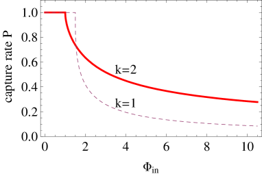
Figure 14: Resonant capture rates for the scaled Hamiltonian (B1) with $k=1$ (first-order resonance) and $k=2$ (second-order resonance).

B.2 First-Order Resonances; $k=1$

The critical values are $\bar{\delta}_{cr}=-3/2$ and $\Phi_{cr}=3/2$. The rate for $\Phi_{in}>\Phi_{cr}$ is given as

$$P_{1}(\Phi_{in})=\frac{2}{1+\frac{\pi}{2\arcsin[(-2\bar{\delta}u/3)^{-3/2}]}},$$ (70)

where the two parameters $\bar{\delta}$ and $u$ are the solutions of the following two equations

$$2\pi\Phi_{in} = \frac{4}{3}\bar{\delta}^{2}\left\{\frac{\pi}{2}+\arcsin\left[\left(\frac{-2\bar{\delta}u}{3}\right)^{-3/2}\right]\right\}$$

$$-\frac{9}{2\bar{\delta}u}\left[\left(\frac{-2\bar{\delta}u}{3}\right)^{3}-1\right]^{1/2}$$

$$-\frac{27}{4\bar{\delta}^{3}u} = 3-u^{2}.$$ (71)

In Fig.14 the capture rate for $k=1$ is shown with the dashed curve.

Appendix C additional canonical transformation

The rescaled Hamiltonians $H$ in Eqs.(49) and (61) are given for the variable $\phi$ (closely related to $\eta$) and its conjugate momentum $\Phi(\propto e^{2})$. The corresponding canonical equations are written as

$$\frac{\partial\phi}{\partial\tau}=\frac{\partial H}{\partial\Phi},~{}~{}\frac{\partial\Phi}{\partial\tau}=-\frac{\partial H}{\partial\phi}.$$ (72)

In the literature, an additional canonical transformation $(\phi,\Phi)\to(x,y)$ is frequently introduced as follows

$$x=\sqrt{2\Phi}\cos\phi,~{}~{}y=\sqrt{2\Phi}\sin\phi.$$ (73)

In the new phase space, the angle between the $x$-axis and the point $(x,y)$ is identical to the original variable $\phi$, and the distance to the origin is proportional to the eccentricity as $\sqrt{x^{2}+y^{2}}\propto\sqrt{\Phi}\propto e$. With these new variables, the rescaled Hamiltonians $H$ become simple polynomials as

$$H=\left(\frac{x^{2}+y^{2}}{2}\right)^{2}+{\bar{\delta}}\frac{x^{2}+y^{2}}{2}+\frac{x^{2}-y^{2}}{2}$$ (74)

for the second-order one (49), and

$$H=\left(\frac{x^{2}+y^{2}}{2}\right)^{2}+{\bar{\delta}}\frac{x^{2}+y^{2}}{2}-\frac{x}{\sqrt{2}}$$ (75)

for the first-order one (61).

The canonical variables $(x,y)$ have geometrically intuitive meanings, and, in many cases, they are more convenient to analyze the dynamics of the rescaled Hamiltonians themselves, as widely done in preceding studies (Borderies & Goldreich 1984; Peale 1986; MD). But we concentrate on the issues more related to the mapping between the Hamiltonians and the EMRI-MBH triple systems, and stay away from the new variables $(x,y)$ in the rest of this paper.

References

- Amaro-Seoane et al. (2012) Amaro-Seoane P., Brem P., Cuadra J., Armitage P. J., 2012, ApJ, 744, L20
- Arun et al. (2009) Arun K. G., Blanchet L., Iyer B. R., Sinha S., 2009, PhRvD, 80, 124018
- Blaes, Lee, & Socrates (2002) Blaes O., Lee M. H., Socrates A., 2002, ApJ, 578, 775