Spatial and luminosity distributions of galactic satellites

Abstract

We investigate the luminosity functions (LFs) and projected number density profiles of galactic satellites around isolated primaries of different luminosity. We measure these quantities for model satellites placed into the Millennium and Millennium II dark matter simulations by the GALFORM semi-analytic galaxy formation model for different bins of primary galaxy magnitude and we investigate their dependence on satellite luminosity. We compare our model predictions to the data of Guo et al. from the Sloan Digital Sky Survey Data Release 8 (SDSS DR8). First, we use a mock light-cone catalogue to verify that the method we used to count satellites in the SDSS DR8 is unbiased. We find that the radial distributions of model satellites are similar to those around comparable primary galaxies in the SDSS DR8, with only slight differences at low luminosities and small projected radii. However, when splitting the satellites by colour, the model and SDSS satellite systems no longer resemble one another, with many red model satellites, in contrast to the dominant blue fraction at similar luminosity in the SDSS. The few model blue satellites are also significantly less centrally concentrated in the halo of their stacked primary than their SDSS counterparts. The implications of this result for the GALFORM model are discussed.

1 Introduction

While the standard $\Lambda$ Cold Dark Matter ($\rm\Lambda CDM$) model has been shown to be in good agreement with observations of large scale structure, the verification of this model at small, galactic scales remains less certain. One reason for this is the increased importance of astrophysical processes relative to gravity in this strongly non-linear regime. The study of the properties and distribution of galactic satellite galaxies provides an opportunity to test $\rm\Lambda CDM$ on small scales while also constraining different aspects of galaxy formation models related to the rates at which satellites form stars, become disrupted and merge with the central galaxy.

The Local Group satellite system within the haloes of the Milky Way (MW) and M31 is often the focus of studies of galactic satellites because it is here where the lowest luminosity satellites can be detected. While this system has been used in attempts to constrain the cosmological model (e.g Bullock et al., 2000; Benson et al., 2002; Klypin et al., 2002; Lovell et al., 2012; Wang et al., 2012), it is not clear that it is typical of the population as a whole. Using the technique of abundance matching in the Millennium II simulation (MS-II), a large-volume, high-resolution dark matter simulation, Boylan-Kolchin et al. (2010) concluded that there should be significant scatter in the properties of satellite systems from one primary to another. This conclusion was supported by Guo et al. (2011) who applied a semi-analytic galaxy formation model to the same simulation. Thus, a large, statistically representative sample of primary galaxies is clearly needed to test cosmological and galaxy formation models. Such an approach also avoids the difficulty of having to define quite what is meant by a Local Group.

The construction of large galaxy redshift surveys, such as the Two Degree Field Galaxy Redshift Survey (2dFGRS, Colless et al., 2001), the SDSS (York et al., 2000), the Galaxy and Mass Assembly (GAMA, Driver et al., 2009, 2011) Survey and the Deep Extragalactic Evolutionary Probe 2 (DEEP2, Davis et al., 2003) Survey, has led to the accumulation of external galaxy samples covering large volumes. Many studies of the luminosity function (LF), spatial distribution and kinematics of bright satellites have been carried out using these and even earlier data sets (e.g. Zaritsky et al., 1993, 1997; van den Bosch et al., 2004; Conroy et al., 2005; van den Bosch et al., 2005; Chen et al., 2006; Koposov et al., 2009; Busha et al., 2010; Prescott et al., 2011). The inclusion of a statistical background subtraction in the satellite system estimators has allowed fainter satellites to be studied using deeper photometric galaxy catalogues (e.g Lorrimer et al., 1994; Liu et al., 2008; Liu et al., 2011; Lares et al., 2011; Guo et al., 2011; Nierenberg et al., 2011; Tal & van Dokkum, 2011; Guo et al., 2012; Jiang et al., 2012; Strigari & Wechsler, 2012; Tal et al., 2012; Wang & White, 2012). By extending the regime over which the satellite distributions have been quantified, a more stringent test of the models can be performed.

While some studies have attempted to make model predictions using cosmological hydrodynamic simulations (e.g Libeskind et al., 2007; Okamoto & Frenk, 2009; Okamoto et al., 2010; Wadepuhl & Springel, 2011; Parry et al., 2012), these efforts are limited to very few primary galaxies because of the high computational cost. The best way to make a statistical sample of model galaxies is by combining large cosmological dark matter simulations, such as the Millennium Simulation (MS, Springel et al., 2005) or the MS-II (Boylan-Kolchin et al., 2009), with a method to include galaxies. This approach was adopted by van den Bosch et al. (2005), who used the conditional luminosity function technique that simultaneously optimizes the model match to the abundance and clustering of low luminosity galaxies in order to study the satellite projected number density profile. Chen et al. (2006) investigated the same statistic by assigning luminosities to dark matter structures so as to match the simulated cumulative circular velocity function to the SDSS cumulative galaxy LF. A similar subhalo abundance matching method was used by Busha et al. (2011) to study the frequency of bright satellites around MW-like primaries.

Semi-analytic models provide a more physically motivated approach to including galaxies into dark matter simulations and have been shown to match a wide variety of observational data (e.g Kauffmann et al., 1993; Lacey et al., 1993; Cole et al., 1994; Kauffmann et al., 1999; Somerville & Primack, 1999; Cole et al., 2000; Benson et al., 2002; Baugh et al., 2005; Bower et al., 2006; Croton et al., 2006; Guo et al., 2011). A large number of studies have used this technique applied to simulations such as the MS-II, Aquarius (Springel et al., 2008) and others to study various aspects of the galaxy population predicted in a $\rm\Lambda CDM$ model (e.g Muñoz et al., 2009; Cooper et al., 2010; Li et al., 2010; Macciò et al., 2010; Font et al., 2011; Wang et al., 2012; Wang & White, 2012). In particular, the mock catalogues constructed by Guo et al. (2011) were tested against data from the SDSS in two studies. Sales et al. (2012) showed that the abundance of satellite galaxies as a function of primary stellar mass in the SDSS DR7 spectroscopic catalogue was in good agreement with this model. Considering fainter dwarf satellites, Wang & White (2012) studied the luminosity, colour distribution and stellar mass function using SDSS DR8 data, concluding that, apart from the model satellites becoming red too quickly when entering the halo of the primary galaxy, many of the observed trends were reproduced in the model.

In this paper, we will test the $\rm{\Lambda CDM}$ model and the semi-analytic galaxy formation model GALFORM (Bower et al., 2006), by comparing the properties of model galactic satellite systems with those measured from the SDSS DR8 spectroscopic and photometric galaxy catalogues. We will introduce a new series of GALFORM model galaxy catalogues based on MS-II that will allow us to extend the predictions from the MS to less luminous galaxies.

In Section 2 we describe the SDSS and model galaxy catalogue data that we use, and compare these two data sets. Section 3 contains summaries of the methods we use to select primaries and determine the satellite luminosity function and the projected number density profile. These two satellite galaxy distributions, upon which we will focus in this paper, were calculated for the SDSS samples by Guo et al. (2011, hereafter Paper I) and Guo et al. (2012, hereafter Paper II). A verification that our estimators are unbiased is performed using the model galaxy samples. The results of the comparison between model satellite systems and those around similarly isolated SDSS primaries is presented in Section 4. Implications for the model drawn from these comparisons are discussed in Section 5; we conclude in Section 6. Throughout the paper we assume a fiducial ${\rm\Lambda CDM}$ cosmological model with $\Omega_{M}=0.3$, $\Omega_{\Lambda}=0.7$ and $H_{0}=70\$km s^-1Mpc^-1.

2 Observed and model galaxies

In this section we briefly review the data being used from the SDSS, which were described in more detail in Paper I and Paper II, before introducing the procedure to construct mock galaxy catalogues to compare with these data.

2.1 SDSS galaxies

Galaxies from both the spectroscopic and photometric samples in the SDSS DR8 are used for this study. Isolated primary galaxies, as defined in Paper I and Paper II, are selected from the spectroscopic survey, whereas satellites can come from either the spectroscopic or photometric surveys. With the relatively poorly constrained distances provided by the photometric redshifts, a statistical background subtraction is performed to obtain an estimate of the satellite galaxy population around each of the primaries, as described in Section 3 below.

2.2 Model galaxies

The model galaxy catalogues were created using a combination of large dark matter simulations to define the mass distribution and a semi-analytic model to place the galaxies within this density field. Either the Millennium Simulation (MS, Springel et al., 2005) or the Millennium-II Simulation (MS-II, Boylan-Kolchin et al., 2009) was used to provide the mass distribution. The former covers a large volume and hence contains many suitable isolated primaries, while the latter traces the mass distribution in a smaller volume, thus resolving structures containing lower luminosity galaxies. While the two simulations trace the same number of particles ($\sim 10^{10}$), the MS and MS-II simulation cubes are $714~{}{\rm Mpc}$ and $143~{}{\rm Mpc}$ long respectively. The corresponding particle masses are $\sim 1.23\times 10^{9}~{}\rm M_{\sun}$ and $9.9\times 10^{6}~{}\rm M_{\sun}$.

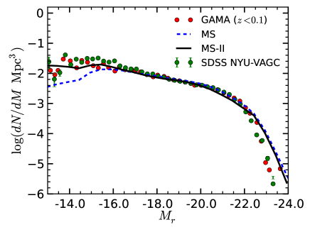
The model galaxies populate the dark matter structures according to the galaxy formation model GALFORM (Bower et al., 2006), which includes reionization at high redshift and energy injection from supernovae and stellar winds in order to prevent the overproduction of low luminosity galaxies. The luminosities of the most luminous galaxies are curbed by feedback from AGN. Parameters in the treatment of the galaxy formation processes have been chosen so as to produce as good a match as possible to the observed K band LF of local galaxies. Fig. 1 shows the luminosity functions of all galaxies in the MS and MS-II simulation cubes. They match quite well with both the observed $r$ band luminosity function of GAMA galaxies (Loveday et al., 2012) shifted to $z=0$ by applying the offset $r={}^{0.1}r-0.22$ (Blanton et al., 2005), and the LF from the SDSS (Blanton et al., 2005). The drop in the MS LF at low luminosities reflects the resolution limit, which corresponds roughly to $M_{r}=-16$. Galaxies placed into the MS-II should be complete significantly beyond this and thus suitable for studying faint satellites.

Figure 1: The luminosity functions of all galaxies in the MS (blue dashed line) and MS-II (black solid line) cubes compared with observed luminosity functions of galaxies in the GAMA survey (the $z<0.1$ subset from Loveday et al. 2012, red points) and SDSS (Blanton et al. 2005, green points). The observed luminosity functions are k-corrected (SDSS) or shifted (GAMA) to $z=0$.

Figure 2: The distribution of estimated $r_{200}$ values for model primary galaxies (solid lines), real $r_{200}$ values for their associated parent haloes (dashed lines) and estimated $r_{200}$ values for primaries selected from the SDSS (dotted lines). From top to bottom, the panels show results for primary magnitude bins centred on $M_{\rm{c}}=-21.0,-22.0$ and $-23.0$ respectively. The vertical lines are the means of the corresponding distributions.

Figure 3: Colour-magnitude diagrams of spectroscopic galaxies in SDSS (top left) and of galaxies in the MS mock light-cone (top right) and the two different simulation cubes (MS, bottom left and MS-II, bottom right). Contours represent lines of constant galaxy number density and the straight lines indicate the colour cuts used to define red and blue primaries. The same cut is used for both the MS and MS-II.

For the MS, in addition to having the GALFORM model galaxies populating the simulation cube, flux-limited light-cone mock catalogues, either with or without the peculiar velocity included in the line-of-sight ‘redshift’, have also been constructed (Merson et al., 2012). These galaxies cover the redshift range $z=0.0-2.0$. To simulate the photometric redshifts in the SDSS DR8 catalogue, we assign a photometric redshift with a random error to every galaxy that is fainter than $m_{r}=17.7$.

Using both the MS and MS-II cubes of galaxies, we can test how robust our results are to the numerical resolution of the dark matter simulations. Comparison of the results obtained from the MS cube with those obtained from the light-cone mock catalogue, provides a test of the accuracy of our background removal and satellite distribution estimation procedures. Finally, the light-cone mock catalogue is intended to mimic the SDSS survey and provide a direct test of the model.

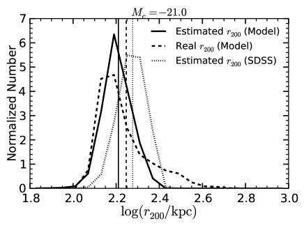
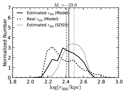
When calculating scaled satellite number density profiles, it is necessary to determine the value of $r_{200}$ (defined as the radius enclosing a mean total overdensity of 200 times the critical cosmic value) associated with each primary galaxy. Following Paper II, $r_{200}$ is estimated from the stellar mass, inferred from the luminosity and colour of the primary. This is converted to a halo mass, $M_{200}$, using the abundance matching technique of Guo et al. (2010), from which $r_{200}$ follows. The solid and dotted lines in Fig. 2 trace the distributions of $r_{200}$ estimated from the MS and SDSS primaries respectively, with the different panels showing results for different luminosity primaries. Vertical lines show the mean values of the distributions, which differ by no more than about $15$ per cent in all cases. This similarity between estimated satellite system sizes in the mock and SDSS suggests that scaling the satellite number density profiles by the system size should not create any large systematic differences between the real and mock results.

The distributions of real $r_{200}$ values, inferred from the dark matter distribution in the simulation cube, are shown with dashed lines in Fig. 2. For the lower luminosity primaries, the real and estimated $r_{200}$ distributions are similar. However, in the bottom panel of Fig. 2 it is apparent that there is a significant population of physically small haloes surrounding primary galaxies whose stellar mass corresponds to a larger halo. As pointed out in Paper II, this is probably due to the fact that the stellar mass varies little with halo mass for these most luminous systems. Thus, any small scatter in stellar mass gives rise to a large change in the value of $r_{200}$ inferred from abundance matching. This is an important source of potential bias when trying to measure concentrations of satellite distributions around the most luminous primaries. In this case, a concentration derived using the value of $r_{200}$ estimated from stellar masses will not necessarily reflect the concentration as defined with respect to the halo mass.

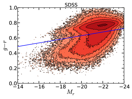
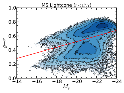
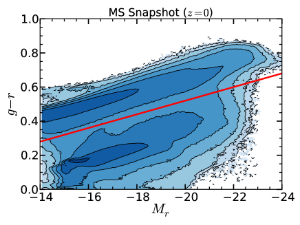
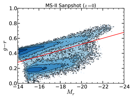
Finally, as we will be investigating the colour dependence of the results, in Fig. 3 we compare the colour distributions of galaxies in the SDSS and model galaxy catalogues. The distribution of SDSS galaxies in the colour-magnitude diagram is shifted along the $g-r$ axis compared to that of the model galaxies. Thus, while we choose ${}^{0.0}(g-r)_{\rm{cut}}^{\rm SDSS}=0.15-0.024M_{r}$ as the line dividing the red and blue populations in the SDSS this boundary is placed at ${}^{0.0}(g-r)_{\rm cut}^{\rm MS,MS-II}=-0.28-0.04M_{r}$ for the model galaxy populations. These cuts are shown in the 4 panels of Fig. 3, where the effect on the colour magnitude distribution of including the survey flux limit can be seen for the MS. This removes the bulk of the low luminosity galaxies that are present in the $z=0$ snapshot and makes the resulting light-cone galaxy population significantly more like that in the SDSS. The fraction of the $-21<M_{r}<-19$ model light-cone galaxies that are defined as red is $0.51$, the same as that for the SDSS. Had we adopted the SDSS colour cut, the model would only have had a red galaxy fraction of $0.28$. For galaxies in the magnitude range $-20<M_{r}<-19$, the red fractions are 0.46 and 0.38 for the model and SDSS respectively, when using the cuts shown in Fig. 3. Thus, apart from a magnitude-dependent shift in the colours of galaxies, which we can correct for with the different colour cuts, the global red galaxy fractions are quite similar between model and SDSS data sets at magnitudes that we will be considering for the satellite galaxies.

The MS and MS-II simulations, once populated with galaxies according to the semi-analytic model, contain very similar galaxy populations. Thus, it is appropriate to use them interchangeably depending upon which is more important: having a large volume containing many primaries, or being able to resolve low luminosity satellite galaxies. However, if we want to compare results from the MS-II cube of galaxies with those from the SDSS flux-limited survey, then we still need to demonstrate, using the MS, that our methods recover from the light-cone mock surveys the same satellite distributions as are present in the simulation cubes.

3 Method

In this section we briefly review the procedure used to determine the satellite LF and projected number density profile for SDSS, described more fully in Papers I and II, before detailing how these distributions are determined from the various different types of model galaxy catalogue. The quality of the recovery of these distributions is quantified by comparing those determined from the MS cube of galaxies with those from the flux-limited mock light-cone surveys.

Primary galaxies are selected to have spectroscopic redshifts in the SDSS and to have magnitudes, $M_{p}$, satisfying $M_{\rm{c}}-\Delta M_{\rm{bin}}<M_{p}<M_{\rm{c}}+\Delta M_{\rm{bin}}$. We choose $M_{\rm{c}}=-21.0,-22.0,-23.0$ and $\Delta M_{\rm{bin}}=0.5$. Further, the primaries should be isolated in the sense that no other galaxy within $\Delta M_{\rm{faint}}=0.5$ magnitudes lies within a projected distance of $2R_{\rm{inner}}$ and is sufficiently close in redshift. ‘Sufficiently close’ is defined as a difference in spectroscopic redshift of less than $\Delta z_{\rm{s}}=0.002$ or, for galaxies without a spectroscopic redshift, with a photometric redshift within $\alpha_{P}\sigma_{P}^{*}$, where $\alpha_{P}=2.5$ and $\sigma_{P}^{*}$ is the photometric redshift error defined in Paper II. $R_{\rm{inner}}$ represents the projected radius within which satellites may reside, and the variable $R_{\rm{outer}}$ defines the outer edge of an annulus within which the local background is estimated. We adopt the same values of $(R_{\rm{inner}},R_{\rm{outer}})$ as in Paper II: $(0.3,0.6),(0.4,0.8)$ and $(0.55,0.9)~{}{\rm Mpc}$ for primaries in magnitude bins $M_{\rm{c}}=-21.0,-22.0$ and $-23.0$ respectively. Only galaxies brighter than $m_{\rm r}^{\rm lim}=20.5$ are considered.

Only sufficiently close galaxies in redshift are included when counting the potential satellites within the projected radius $R_{\rm{inner}}$ and making the local background estimate from the surrounding annulus out to $R_{\rm{outer}}$. The background-subtracted satellite systems are stacked for primaries in each absolute magnitude bin to provide estimates for the mean satellite LFs and projected number density profiles of satellites more luminous than a particular absolute magnitude, as described more fully in Papers I & II.

The procedure described above is applied to the SDSS itself and also to the MS redshift space light-cone mock catalogue. However, different estimation procedures are used for the light-cone mock with real space (rather than redshift space) galaxy coordinates and the galaxy populations in the simulation cubes. With the real space positions, it is possible to define isolated primaries as having no bright neighbours within a sphere of radius $2R_{\rm{inner}}$. The satellites within a sphere of radius $R_{\rm{inner}}$ can also be determined without any need for background subtraction. Using only the real space satellites, the estimation of the satellite luminosity function is straightforward. For the $j$th magnitude bin, the average satellite LF is estimated using

$$\overline{N}^{\rm real\ sat}_{j}=\frac{\Sigma_{i}N^{\rm real\ sat}_{i}(M_{j})}{N_{j}^{\rm real\ prim}},$$ (1)

where $N^{\rm real\ sat}_{i}$ is the number of satellites around primary $i$ and $N_{j}^{\rm real\ prim}$ is the number of primaries contributing to the $j$th bin of the LF.

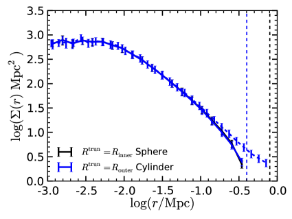
While we need no correction for interlopers in real space, the process of estimating the mean projected number density of satellite galaxies is such that a fair comparison with light-cone data still requires the subtraction of a background estimated from an outer area. Hence, the projected number density profiles of satellites brighter than $M^{\rm trun}$ in real space are determined using all galaxies within a cylinder of projected radius $R_{\rm{outer}}$ and length $2R_{\rm{outer}}$, centred on the primary. These galaxies are projected onto a plane and provide the sources for the potential satellites/background for projected radii less/greater than $R_{\rm{inner}}$. The projected number density profile is determined using

$$\overline{\Sigma}_{i}(r^{\rm ann}_{j})=\frac{\sum_{i}N_{ij}(M^{\rm trun})}{\sum_{i}A_{ij}^{\rm p}}-\frac{\sum_{i}N^{\rm bck}_{i}}{\sum_{i}A^{\rm outer}_{i}},$$ (2)

where $N_{ij}$ is the number of galaxies brighter than $M^{\rm trun}$ within a projected distance $R_{\rm{inner}}$ of the $i$th primary and in the $j$th projected annulus, and $N^{\rm bck}_{i}$ is the corresponding number of galaxies in the projected outer annulus, $R_{\rm{inner}}<r<R_{\rm{outer}}$. $A_{ij}^{\rm p}$ is the area contributed by the $i$th primary to the $j$th annulus for the detection of satellites brighter than $M^{\rm trun}$,

$$A_{ij}^{\rm p}(M^{\rm trun})=\left\{\begin{array}[]{ll}A_{ij}&M^{\rm trun}<M_{i}^{\rm{lim}}\\ 0&M^{\rm trun}>M_{i}^{\rm{lim}}\ ,\end{array}\right.$$ (3)

where $A_{ij}$ is the area of the $j$th annulus surrounding the $i$th primary and $M_{i}^{\rm lim}$ is the absolute magnitude that corresponds to the apparent magnitude limit of the mock catalogue. $A_{i}^{\rm outer}$ is the corresponding area in the outer annulus surrounding the $i$th primary.

The comparison of the projected number density profiles, before and after background subtraction, with that formed by simply projecting the galaxies within a sphere of radius $R_{\rm{inner}}$ of the primary galaxy is shown in Fig. 4. The results indicate that the projected profile after subtracting the background very accurately recovers that estimated directly from the galaxies within the inner area ($r<R_{\rm{inner}}$). The impact of the background subtraction is small and limited to radii near to $R_{\rm{inner}}$. This establishes that the method for calculating the background subtracted projected number density profile from a real space light-cone survey provides an unbiased estimate of that produced when only satellites within a 3D distance $R_{\rm{inner}}$ are used. We can now compare these real space profiles with those from redshift space light-cones.

Figure 4: The comparison of real space projected number density profiles estimated by different methods. The black line is the profile estimated by projecting the satellites within spheres of radius $R_{\rm{inner}}$ around primaries. The dashed blue curve shows the projected number density profile of all galaxies within a line-of-sight distance $R_{\rm{outer}}$ of a primary. The solid blue curve is the background-subtracted case, where the background is estimated from the outer annulus with $R_{\rm{inner}}<r<R_{\rm{outer}}$. Vertical dashed lines show $R_{\rm{inner}}$ and $R_{\rm{outer}}$.

Figure 5: Satellite LFs (top) and number density profiles (bottom) estimated from light-cone mock catalogues and directly from the MS cube. The results for primary magnitude bins centred at $M_{\rm{c}}=-21.0,-22.0,-23.0$ are shown in black, blue and red respectively. Solid and dashed lines correspond to results from redshift and real space light-cones respectively, whereas the points show the results for the whole volume in the simulation cube.

Having described the three different types of model galaxy catalogues made using the MS and how the satellite distributions are determined from each of them, we are now in a position to test the accuracy of our estimation procedure. Fig. 5 shows the satellite LF and projected number density profiles estimated from each of the model galaxy catalogues: simulation cube, real space light-cone and redshift space light-cone. The agreement between the two different satellite distributions measured from all three catalogues at $M_{\rm{c}}=-21.0,-22.0$ and $-23.0$ provides strong support that our results are unbiased, and that our technique for background subtraction is appropriate. Given that the isolated primaries are a specially selected subset of the differentially clustered galaxy population, one would expect that a local, rather than global, background subtraction would be appropriate. The fact that the results from the MS light-cone mock match well with those from the MS cube of galaxies suggests that we can use results from the MS-II simulation cube at $z=0$ when comparing with low luminosity galaxies in the SDSS DR8.

Figure 6: Model (MS-II, solid lines) and SDSS (points) satellite LFs (top), projected number density profiles (middle) and normalized profiles (bottom). The results for primary luminosity bins $M_{\rm{c}}=-21.0,-22.0,-23.0$ are shown in black, blue and red, respectively.

Figure 7: The dependence of the scaled and unscaled satellite density profiles on satellite luminosity for primaries in the range $-22.5<M_{\rm p}<-21.5$. Unscaled (top) and scaled (middle) profiles of satellites are shown for two different luminosity bands: $-21.0<M_{s}<-19.0$ (black) and $-19.0<M_{s}<-17.0$ (blue). The solid lines and points correspond to results from the model and SDSS respectively. The bottom panel shows scaled profiles for lower luminosity satellites in the model.

4 Results

Having verified that the model galaxies have similar distributions of luminosity and colour to those in the SDSS and that our local background subtraction procedure produces unbiased estimates of the satellite LF and projected number density profile, we now compare the model and observed satellite systems in more detail.

4.1 Dependence on primary and satellite luminosity

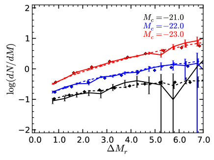
The top panel of Fig. 6 shows the satellite LFs for the primary magnitude bins $M_{\rm{c}}=-21.0,-22.0,-23.0$ estimated from both the SDSS and MS-II mock data. For $\Delta M_{r}<5$, the model and SDSS satellite luminosity functions generally agree well. However, there is a steepening of the LF for lower luminosity satellite galaxies in the SDSS that is not present in the model. The MS-II was used for this comparison, so a lack of numerical resolution should not be responsible for this deficit.

The middle panel of Fig. 6 shows the projected number density profiles of satellites brighter than $M_{\rm sat}^{\rm trun}=-19.0$ for the different primary samples. This limit is chosen, following Paper II, to ensure that the profiles for different luminosity bins are measured from a large enough sample. In all cases the profile approximately follows $\Sigma(r)\propto r^{-1.5}$, with the amplitude reflecting the fact that more luminous primaries host more satellites. For most radii, the model reproduces the amplitude observed in SDSS. In detail though, there is a factor 2 difference at $\sim 30~{}{\rm kpc}$ for both $M_{\rm{c}}=-21.0$ and $-23.0$. The model underproduces satellites at this radius for the least luminous primaries and overproduces them for the most luminous primaries.

Once rescaled in both radius and projected number density, as shown in the bottom panel of Fig. 6, the model and SDSS profiles line up well outside the region at $0.05\mathrel{\hbox{\hbox to0.0pt{\hbox{\lower 4.0pt\hbox{$\sim$}}\hss}\hbox{$<$}}}r/r_{200}\mathrel{\hbox{\hbox to0.0pt{\hbox{\lower 4.0pt\hbox{$\sim$}}\hss}\hbox{$<$}}}0.1$. As noted in Paper II, the slight deficit of satellite galaxies in the inner regions of the SDSS for $M_{\rm{c}}=-23.0$ primaries, relative to the model, may reflect difficulties identifying low luminosity satellites in regions where the background light subtraction is significant (Aihara et al., 2011). This had the effect of slightly decreasing the fitted concentration of satellites around the most luminous primaries relative to the low luminosity primary bins.

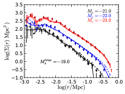
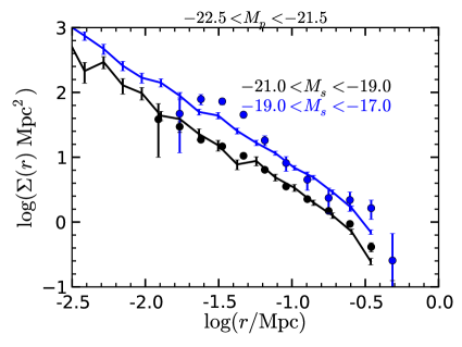
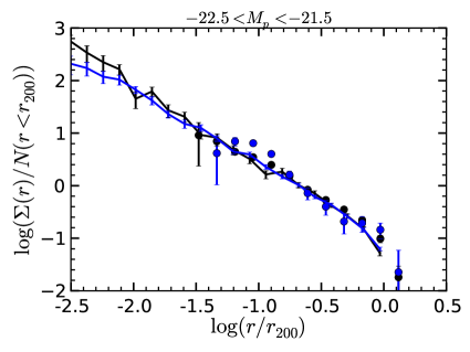
The dependence of the satellite projected number density profile on satellite luminosity for primaries with $-22.5<M_{p}<-21.5$ is shown in Fig. 7. Satellites are split into two bands of luminosity: $-21.0<M_{s}<-19.0$, representing the objects that contributed to the profile in Fig. 6, and $-19.0<M_{s}<-17.0$, showing the behaviour of lower luminosity satellites. The top and middle panels show the satellite projected number density profiles before and after scaling respectively. While generally in good agreement, there is an excess of lower luminosity satellites in the SDSS relative to the model at $\sim 30~{}{\rm kpc}$.

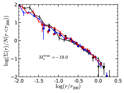
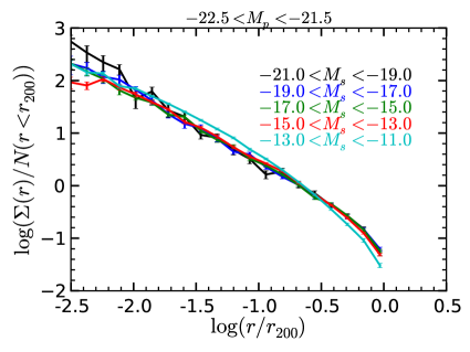
The ‘bump’ in the projected number density profile in the SDSS data is present only for the lower luminosity satellites. One is therefore tempted to ask if it is present at any satellite luminosity in the mock catalogues. This question is answered in the bottom panel of Fig. 7, where no comparable deviations are seen for satellites with $M_{s}<-13$, which have indistinguishable profiles from those of brighter satellites. The profile for satellites with $-13<M_{s}<-11$ shows a slight change in shape over a large range of scales relative to the other sets of satellites, but nothing as pronounced as is seen in the SDSS.

4.2 Dependence on primary and satellite colour

Figure 8: The dependence on primary galaxy colour of the satellite LF (top), unscaled (middle) and scaled (bottom) number density profiles for primary galaxies of magnitude $-22.5<M_{p}<-21.5$. Solid and dashed lines show model results for primaries in the MS and MS-II respectively, whereas the points are for SDSS. All profiles are for satellites more luminous than $M_{s}=-19.0$.

Figure 9: Dependence of satellite distributions on the colour of the satellite galaxy. Symbols and line types have the same meaning as in Fig. 8.

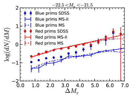
As a further test of the galaxy formation model, which has so far largely succeeded in reproducing the satellite LF and projected number density distributions, we now split the primaries and satellites by colour using the slightly different colour cuts described in Section 2.2 for the model and SDSS.

Fig. 8 shows how the satellite luminosity function and projected number density profile depend upon the colour of the primary around which they are being measured, and compares the results from the model and the SDSS for primaries with $-22.5<M_{p}<-21.5$. For the adopted colour cuts, the vast majority of primaries are classified as red in both the model and SDSS. Given that when not split by colour the model produces a good match to these satellite distributions, it is no surprise that the satellite populations around red primaries agree well between model and observations. However, the blue primaries in the mock catalogues are deficient in satellites by a factor of $2-3$. The excess satellites around SDSS primaries span the range of luminosities and radii being considered here, with a slight tendency to be at lower luminosity and nearer to the primary than for the satellites present around the model primaries. The scaled profiles in the bottom panel of Fig. 8 show that satellites around blue SDSS primaries are slightly more concentrated than those around model primaries.

In the top two panels of Fig. 8 results for both the MS and MS-II are shown. Because of its limited resolution the LF in the MS becomes incomplete at $\Delta M\sim 5.5$, but the LF in the MS-II is well resolved down to $\Delta M\sim 7$. On the other hand, in the smaller volume of the MS-II, there is a relatively small number of primaries and, as a result, the projected number density profile of satellites brighter than $M_{s}=-19$ is noisy (and it is therefore omitted in the lower panel of the figure). In the regions where both simulations are well resolved and sampled, their results are consistent.

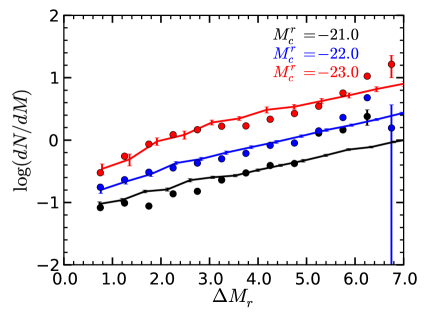
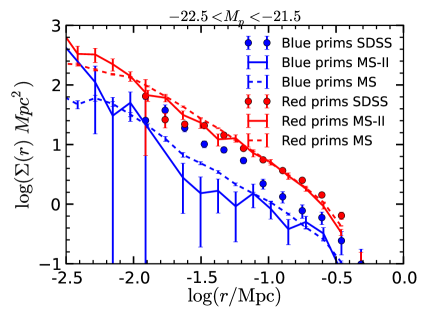
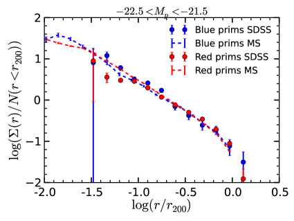
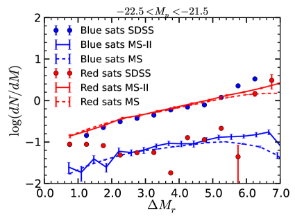
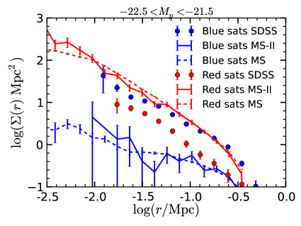
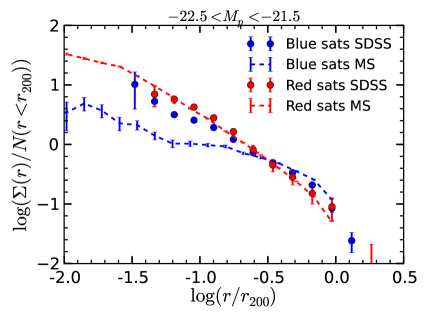
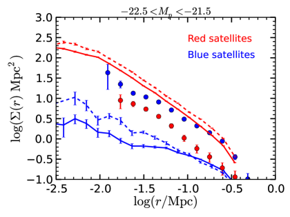
The satellites themselves can be divided into red and blue subsets and their distributions around primaries with $-22.5<M_{p}<-21.5$ are shown in Fig. 9. Once again both MS and MS-II results are shown in the top two panels, while the noisy MS-II results are not presented for the scaled projected number density profiles in the bottom panel. The fact that the colour cuts in the model and SDSS samples yield completely different red and blue fractions is immediately apparent in the satellite LFs, with the model satellite systems dominated by red satellites to a coincidentally similar extent as the blue satellites dominate around SDSS primaries. For the most luminous satellites, the SDSS blue and red fractions converge, whereas this does not happen for the model.

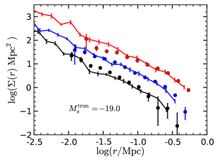
The shape of the projected density profiles of red satellites are very similar for the model and SDSS systems, once the difference in amplitude has been scaled away, as shown in the bottom panel of Fig. 9. However, this is not the case for the blue satellites, which have a much less concentrated distribution around model primaries. For real systems of blue satellites, the distribution is only slightly less concentrated than it is for the red satellites.

5 Discussion

The comparison of galactic satellite systems in the model with those in the SDSS shows that the dependence of the satellite distributions on primary and satellite luminosity is captured quite well by the GALFORM model. This is a non-trivial success of the model since its parameters were adjusted merely to match the global K-band LF of galaxies, with no direct reference to satellite systems. There is an excess of very low luminosity satellites around SDSS primaries relative to the model, and the projected number density profiles are up to a factor 2 discrepant within $\sim 30~{}{\rm kpc}$, but the agreement is generally good.

Tal et al. (2012) also studied the radial distribution of satellite systems around bright primary galaxies using SDSS data. Their primaries were LRGs at $0.28<z<0.40$ with no isolation criteria applied and hence often in groups of bright galaxies, and thus are different to those studied here in a few respects that may well be important. They found the projected number density was well fitted by a combination of a projected NFW profile (Navarro et al., 1996, 1997) for large radii and a central steeper profile that follows the stacked light profile of the LRGs. This central bump is similar to that seen for the lower luminosity satellites around primary galaxies shown in Fig. 7, but is, in contrast, most apparent in the high luminosity satellites around the LRGs.

The differences between the model and SDSS satellite systems are greater when the colour of the satellites is considered. Even the distribution of galaxies in the colour-magnitude plane shows that the model has too high a fraction of low luminosity red galaxies relative to the SDSS. The model blue satellites are both significantly depleted and very much less concentrated relative to either blue or red SDSS satellites, which have a projected number density profile like that of the red model satellites. These pieces of evidence point to the model being too ready to convert low luminosity blue galaxies to red ones.

Figure 10: The effect on the model satellite LF (top) and number density profiles (lower two panels) of changing the treatment of hot gas stripping in GALFORM for primary galaxies of magnitude $-22.5<M_{p}<-21.5$. The points are the results measured from SDSS data, whereas solid and dashed lines are the results measured from catalogues constructed using the Bower et al. (2006) and Font et al. (2008) GALFORM models respectively. The middle panel shows the profiles of all satellites, whereas the lower panel shows them split by colour.

Weinmann et al. (2012) suggest that galaxy formation models have a generic problem with maintaining sufficient gas to form stars in lower mass galaxies at low redshift. The satellite galaxies we are considering are somewhat larger than those studied by Weinmann et al. (2012), and our choice of different colour cuts for defining red and blue galaxies in the model and SDSS samples reduces global systematic colour differences. For instance, the overall fraction of blue galaxies in the model, at the magnitudes of the satellites that we focus on, is very similar to that in the SDSS. Satellite galaxies in our study constitute only a small fraction of the total population of galaxies. Thus, a dramatic change in the satellite properties will leave very little imprint on the global LF.

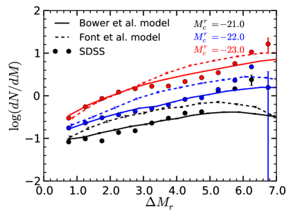
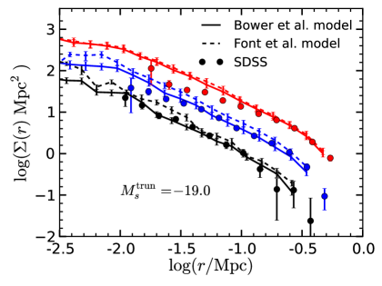
Alternatively, it could be that semi-analytical galaxies turn red too rapidly after accretion into larger haloes. This idea was investigated by Font et al. (2008), who changed the GALFORM treatment of gas stripping from subhaloes as they enter the virial radius of large primary galaxies. Rather than hot gas being stripped from subhaloes immediately as they enter the virial radius, a more gradual loss of gas is adopted in the Font et al. (2008) model. This allows a relatively extended period of star formation to occur and the possiblity of bluer satellites. We have performed our analysis on a model galaxy population constructed using this particular variant of the Bower et al. (2006) GALFORM model. While the typical colours of galaxies do become slightly bluer, the number of blue satellites per primary in the Font et al. (2008) model increases only slightly, as can be seen in Fig. 10. The shape of the blue satellite profile improves significantly, with the extra blue satellites being found preferentially at small radii. However, the abundance of red satellites is also increased by this modification to the GALFORM model, because satellites generally become more luminous as a result of the more extended period of star formation. As a result, the Font et al. (2008) model overproduces satellite abundances overall, as shown in the upper two panels of Fig. 10. The overproduction is most discrepant with the data at low luminosities.

Many important astrophysical processes combine to determine the distribution of low luminosity galaxies. Therefore the distributions of satellite galaxies will depend sensitively on aspects of the galaxy formation model. Given that the treatment of gas stripping can have the large impact shown in Fig. 10, one is drawn to conclude that the ability of the default Bower et al. (2006) model to match the total satellite LF and projected number density profile of the SDSS systems was far from inevitable.

6 Conclusions

Using model galaxy catalogues constructed using large dark matter simulations and a semi-analytic galaxy formation model, we have tested the accuracy of our procedures for measuring properties of the distribution of satellite galaxies around bright, isolated primary galaxies. We find that our local estimation of the abundance of background galaxies yields unbiased estimates of the satellite galaxy luminosity function and projected number density profile. The agreement between results in the MS and MS-II galaxy catalogues in their region of overlap shows that our results are numerically converged and allows us to extend the dynamic range of the model predictions.

Comparing the model predictions with those measured for satellite systems in the SDSS, we find that the dependence of the satellite LF is matched well for $M_{\rm{c}}=-21.0,-22.0,-23.0$ and $\Delta M_{r}<5$. Lower luminosity satellites are increasingly underpredicted by the model. The projected number density profile is also well reproduced at radii greater than $\sim 30~{}{\rm kpc}$. At smaller radii, deviations in the abundance by a factor of two are apparent. These differences between model and SDSS are seen most strongly in the low luminosity satellites, which show an excess in the SDSS relative to the extrapolation of the power law from larger radii, which describes the inner regions of the model satellite systems.

Splitting the sample into red and blue galaxies produces more dramatic differences between the model and SDSS results. The model places a factor $2-3$ fewer satellites around blue primaries than are present around comparable SDSS primaries. However, the discrepancy between model and SDSS is even larger when considering the colours of the satellites. The model satellites are predominantly red, in contrast to the blue-dominated SDSS satellite galaxy population. Furthermore, what model blue satellites there are have a significantly more extended distribution around their primary galaxy than is seen for either the SDSS blue satellites or the red satellites in the model and SDSS.

The generally successful comparison of the GALFORM model with the SDSS data performed here provides a non-trivial validation of the assumptions and framework of this kind of modelling. At the same time, the failure of the model to account for the observed colour dependence of the satellite properties demonstrates that the model is incomplete and that important physical processes, almost certainly related to the rapidity with which infalling satellite galaxies turn red, are not being faithfully modelled. Since a similar shortcoming is present in the independent model of Guo et al. (2011), this problem seems deep-rooted and is worthy of further investigation.

References

- Aihara et al. (2011) Aihara H. et al., 2011, ApJS, 193, 29
- Baugh et al. (2005) Baugh C. M., Lacey C. G., Frenk C. S., Granato G. L., Silva L., Bressan A., Benson A. J., Cole S., 2005, MNRAS, 356, 1191
- Benson et al. (2002) Benson A. J., Frenk C. S., Lacey C. G., Baugh C. M., Cole S., 2002, MNRAS, 333, 177
- Blanton et al. (2005) Blanton M. R., Lupton R. H., Schlegel D. J., Strauss M. A., Brinkmann J., Fukugita M., Loveday J., 2005, ApJ, 631, 208
- Bower et al. (2006) Bower R. G., Benson A. J., Malbon R., Helly J. C., Frenk C. S., Baugh C. M., Cole S., Lacey C. G., 2006, MNRAS, 370, 645
- Boylan-Kolchin et al. (2010) Boylan-Kolchin M., Springel V., White S. D. M., Jenkins A., 2010, MNRAS, 406, 896
- Boylan-Kolchin et al. (2009) Boylan-Kolchin M., Springel V., White S. D. M., Jenkins A., Lemson G., 2009, MNRAS, 398, 1150
- Bullock et al. (2000) Bullock J. S., Kravtsov A. V., Weinberg D. H., 2000, ApJ, 539, 517
- Busha et al. (2010) Busha M. T., Alvarez M. A., Wechsler R. H., Abel T., Strigari L. E., 2010, ApJ, 710, 408
- Busha et al. (2011) Busha M. T., Wechsler R. H., Behroozi P. S., Gerke B. F., Klypin A. A., Primack J. R., 2011, ApJ, 743, 117
- Chen et al. (2006) Chen J., Kravtsov A. V., Prada F., Sheldon E. S., Klypin A. A., Blanton M. R., Brinkmann J., Thakar A. R., 2006, ApJ, 647, 86
- Cole et al. (1994) Cole S., Aragon-Salamanca A., Frenk C. S., Navarro J. F., Zepf S. E., 1994, MNRAS, 271, 781
- Cole et al. (2000) Cole S., Lacey C. G., Baugh C. M., Frenk C. S., 2000, MNRAS, 319, 168
- Colless et al. (2001) Colless M. et al., 2001, MNRAS, 328, 1039
- Conroy et al. (2005) Conroy C. et al., 2005, ApJ, 635, 982
- Cooper et al. (2010) Cooper A. P. et al., 2010, MNRAS, 406, 744
- Croton et al. (2006) Croton D. J. et al., 2006, MNRAS, 365, 11
- Davis et al. (2003) Davis M. et al., 2003, in Guhathakurta P., ed., Society of Photo-Optical Instrumentation Engineers (SPIE) Conference Series Vol. 4834, Society of Photo-Optical Instrumentation Engineers (SPIE) Conference Series. pp 161–172
- Driver et al. (2011) Driver S. P. et al., 2011, MNRAS, 413, 971
- Driver et al. (2009) Driver S. P. et al., 2009, Astronomy and Geophysics, 50, 050000
- Font et al. (2011) Font A. S. et al., 2011, MNRAS, 417, 1260
- Font et al. (2008) Font A. S. et al., 2008, MNRAS, 389, 1619
- Guo et al. (2011) Guo Q., Cole S., Eke V., Frenk C., 2011, MNRAS, 417, 370, Paper I
- Guo et al. (2012) Guo Q., Cole S., Eke V., Frenk C., 2012, ArXiv e-prints, Paper II
- Guo et al. (2011) Guo Q. et al., 2011, MNRAS, 413, 101
- Guo et al. (2010) Guo Q., White S., Li C., Boylan-Kolchin M., 2010, MNRAS, 404, 1111
- Jiang et al. (2012) Jiang C., Jing Y., Li C., 2012, ArXiv e-prints
- Kauffmann et al. (1999) Kauffmann G., Colberg J. M., Diaferio A., White S. D. M., 1999, MNRAS, 303, 188
- Kauffmann et al. (1993) Kauffmann G., White S. D. M., Guiderdoni B., 1993, MNRAS, 264, 201
- Klypin et al. (2002) Klypin A., Zhao H., Somerville R. S., 2002, ApJ, 573, 597
- Koposov et al. (2009) Koposov S. E., Yoo J., Rix H.-W., Weinberg D. H., Macciò A. V., Escudé J. M., 2009, ApJ, 696, 2179
- Lacey et al. (1993) Lacey C., Guiderdoni B., Rocca-Volmerange B., Silk J., 1993, ApJ, 402, 15
- Lares et al. (2011) Lares M., Lambas D. G., Domínguez M. J., 2011, AJ, 142, 13
- Li et al. (2010) Li Y.-S., De Lucia G., Helmi A., 2010, MNRAS, 401, 2036
- Libeskind et al. (2007) Libeskind N. I., Cole S., Frenk C. S., Okamoto T., Jenkins A., 2007, MNRAS, 374, 16
- Liu et al. (2008) Liu C., Hu J., Newberg H., Zhao Y., 2008, A&A, 477, 139
- Liu et al. (2011) Liu L., Gerke B. F., Wechsler R. H., Behroozi P. S., Busha M. T., 2011, ApJ, 733, 62
- Lorrimer et al. (1994) Lorrimer S. J., Frenk C. S., Smith R. M., White S. D. M., Zaritsky D., 1994, MNRAS, 269, 696
- Loveday et al. (2012) Loveday J. et al., 2012, MNRAS, 420, 1239
- Lovell et al. (2012) Lovell M. R. et al., 2012, MNRAS, 420, 2318
- Macciò et al. (2010) Macciò A. V., Kang X., Fontanot F., Somerville R. S., Koposov S., Monaco P., 2010, MNRAS, 402, 1995
- Merson et al. (2012) Merson A. I. et al., 2012, ArXiv e-prints
- Muñoz et al. (2009) Muñoz J. A., Madau P., Loeb A., Diemand J., 2009, MNRAS, 400, 1593
- Navarro et al. (1996) Navarro J. F., Frenk C. S., White S. D. M., 1996, ApJ, 462, 563
- Navarro et al. (1997) Navarro J. F., Frenk C. S., White S. D. M., 1997, ApJ, 490, 493
- Nierenberg et al. (2011) Nierenberg A. M., Auger M. W., Treu T., Marshall P. J., Fassnacht C. D., 2011, ApJ, 731, 44
- Okamoto & Frenk (2009) Okamoto T., Frenk C. S., 2009, MNRAS, 399, L174
- Okamoto et al. (2010) Okamoto T., Frenk C. S., Jenkins A., Theuns T., 2010, MNRAS, 406, 208
- Parry et al. (2012) Parry O. H., Eke V. R., Frenk C. S., Okamoto T., 2012, MNRAS, 419, 3304
- Prescott et al. (2011) Prescott M. et al., 2011, MNRAS, 417, 1374
- Sales et al. (2012) Sales L. V., Wang W., White S. D. M., Navarro J. F., 2012, MNRAS, p. 31
- Somerville & Primack (1999) Somerville R. S., Primack J. R., 1999, MNRAS, 310, 1087
- Springel et al. (2008) Springel V. et al., 2008, MNRAS, 391, 1685
- Springel et al. (2005) Springel V. et al., 2005, Nature, 435, 629
- Strigari & Wechsler (2012) Strigari L. E., Wechsler R. H., 2012, ApJ, 749, 75
- Tal & van Dokkum (2011) Tal T., van Dokkum P. G., 2011, ApJ, 731, 89
- Tal et al. (2012) Tal T., Wake D. A., van Dokkum P. G., 2012, ApJ, 751, L5
- van den Bosch et al. (2004) van den Bosch F. C., Norberg P., Mo H. J., Yang X., 2004, MNRAS, 352, 1302
- van den Bosch et al. (2005) van den Bosch F. C., Yang X., Mo H. J., Norberg P., 2005, MNRAS, 356, 1233
- Wadepuhl & Springel (2011) Wadepuhl M., Springel V., 2011, MNRAS, 410, 1975
- Wang et al. (2012) Wang J., Frenk C. S., Cooper A. P., 2012, ArXiv e-prints
- Wang et al. (2012) Wang J., Frenk C. S., Navarro J. F., Gao L., Sawala T., 2012, MNRAS, 424, 2715
- Wang & White (2012) Wang W., White S. D. M., 2012, MNRAS, 424, 2574
- Weinmann et al. (2012) Weinmann S. M., Pasquali A., Oppenheimer B. D., Finlator K., Mendel J. T., Crain R. A., Macciò A. V., 2012, MNRAS, 426, 2797
- York et al. (2000) York D. G. et al., 2000, AJ, 120, 1579
- Zaritsky et al. (1993) Zaritsky D., Smith R., Frenk C., White S. D. M., 1993, ApJ, 405, 464
- Zaritsky et al. (1997) Zaritsky D., Smith R., Frenk C. S., White S. D. M., 1997, ApJ, 478, L53