Geometric engineering of (framed) BPS states

Abstract.

BPS quivers for ${\mathcal{N}}=2$ $SU(N)$ gauge theories are derived via geometric engineering from derived categories of toric Calabi-Yau threefolds. While the outcome is in agreement of previous low energy constructions, the geometric approach leads to several new results. An absence of walls conjecture is formulated for all values of $N$, relating the field theory BPS spectrum to large radius D-brane bound states. Supporting evidence is presented as explicit computations of BPS degeneracies in some examples. These computations also prove the existence of BPS states of arbitrarily high spin and infinitely many marginal stability walls at weak coupling. Moreover, framed quiver models for framed BPS states are naturally derived from this formalism, as well as a mathematical formulation of framed and unframed BPS degeneracies in terms of motivic and cohomological Donaldson-Thomas invariants. We verify the conjectured absence of BPS states with “exotic” $SU(2)_{R}$ quantum numbers using motivic DT invariants. This application is based in particular on a complete recursive algorithm which determines the unframed BPS spectrum at any point on the Coulomb branch in terms of noncommutative Donaldson-Thomas invariants for framed quiver representations.

1. Introduction

The BPS spectrum of four dimensional ${\mathcal{N}}=2$ gauge theories has been a constant subject of research since the discovery of the Seiberg-Witten solution. An incomplete sampling of references includes [125, 126, 61, 22, 101, 23, 112, 113, 127, 65, 85, 131]. Very recent intense activity in this field was motivated by the connection [67] between wallcrossing on the Coulomb branch and the Kontsevich-Soibelman formula [106]. An incomplete sampling of references includes [67, 70, 38, 68, 37, 2, 3, 39, 69, 34, 36, 35, 137]. For recent reviews see [115, 33].

On the other hand, it has been known for a while that many ${\mathcal{N}}=2$ gauge theories are obtained in geometric engineering as a low energy limit of string theory dynamics in the presence of Calabi-Yau singularities [5, 96, 101, 99, 98]. This leads immediately to a close connection between the gauge theory BPS spectrum and the BPS spectrum of string theory in the presence of such singularities. The latter consists of supersymmetric D-brane bound states wrapping exceptional cycles, and hence can in principle be analyzed using derived category methods [104, 56, 57, 8, 128, 12, 7]. In principle geometric engineering is expected to provide a microscopic string theory derivation for the BPS quivers found in [47, 48, 37, 3] by low energy methods. Indeed the BPS quivers constructed in loc. cit. for $SU(N)$ gauge theories were first derived by Fiol in [62] using fractional branes on quotient singularities. It is quite remarkable that this construction was confirmed ten years later by completely different low energy methods. A similar approach, employing a more geometric point of view has been subsequently employed in [10, 54] for $SU(2)$ gauge theories. Their results are again in agreement with the low energy constructions.

The goal of the present work is to proceed to a systematic study of the gauge theory BPS spectrum via categorical and geometric methods. Special emphasis is placed on higher rank gauge theories, where the BPS spectrum is not completely known on the entire Coulomb branch, many problems being at the moment open. In order to keep the paper to be of reasonable length, only pure $SU(N)$ gauge theories will be considered in this paper. In this case the local toric threefolds are resolved $A_{N-1}$ quotient singularities fibered over $\mathbb{P}^{1}$, such that the singularity type does not jump at any points on the base. Their derived categories are equivalent by tilting to derived categories of modules over the path algebra of a quiver with potential determined by an exceptional collection of line bundles. Physically, these quivers encode the quantum mechanical effective action of a collection of fractional branes on the toric threefold. Taking the field theory limit amounts to a truncation of the fractional brane quiver, omitting the branes which become very heavy in this limit together with the adjacent arrows. The resulting quiver for pure $SU(N)$ gauge theory is of the form

with a potential

$${\mathcal{W}}=\sum_{i=1}^{N-2}\left[r_{i}(a_{i}c_{i}-c_{i+1}b_{i})+s_{i}(a_{i}d_{i}-d_{i+1}b_{i})\right].$$

This is the same as the quiver found in [62], and is mutation equivalent to the quivers found in [37, 3] by different methods. This approach can be extended to gauge theories with flavors allowing the $A_{N-1}$ singularity to jump at special points on the base.

In order to set the stage, geometric engineering and the field theory limit of Calabi-Yau compactifications is carefully reviewed in Section 2. Special emphasis is placed on categorical constructions, in particular exceptional collections of line bundles on toric Calabi-Yau threefolds. In particular an explicit construction of such collections is provided for toric Calabi-Yau threefolds $X_{N}$ engineering pure $SU(N)$ gauge theory. Not surprisingly, it is then shown that the associated fractional brane quiver is the same as the one obtained in [62] by orbifold methods. As opposed to the construction in loc. cit., the geometric approach provides a large radius limit presentation of fractional branes in terms of derived objects on $X_{N}$. The main outcome of Section 2 is a conjectural categorical description of gauge theory BPS states in terms of a triangulated subcategory ${\mathcal{G}}\subset D^{b}(X_{N})$. As shown by detailed A-model computations in Section 2.3, ${\mathcal{G}}$ is a truncation of $D^{b}(X_{N})$ generated by fractional branes with finite central charges in the field theory limit. It is perhaps worth noting that this conclusion involves certain delicate cancellations between tree level and world-sheet instanton contributions which were never spelled out in the literature.

According to [56, 57, 8] supersymmetric D-brane configurations on $X_{N}$ are identified with $\Pi$-stable objects in the derived category $D^{b}(X_{N})$, or in rigorous mathematical formulation, Bridgeland stable objects [28]. Therefore one is naturally led to conjecture that gauge theory BPS states will be constructed in terms of Bridgeland stable objects in $D^{b}(X_{N})$ which belong to ${\mathcal{G}}$. However it is important to note that agreement of the low energy constructions with [37, 2, 3] requires a stronger statement. Namely, that gauge theory BPS states must be constructed in terms of an intrinsic stability condition on ${\mathcal{G}}$. Mathematically, these two statements are not equivalent since in general a stability condition on the ambient derived category does not automatically induce one on the subcategory ${\mathcal{G}}$. It is however shown in Section 2.4 that this does hold for quivery or algebraic stability conditions, analogous to those constructed in [27, 15]. The above statement fails for geometric large radius limit stability conditions, such as $(\omega,B)$-stability, which is analyzed in Section 4. Section 2 concludes with a detailed comparison of gauge theoretic BPS indices and the motivic Donaldson-Thomas invariants constructed in [106]. In particular it is shown that the protected spin characters defined in [68] correspond mathematically to a $\chi_{y}$-genus type specialization of the motivic invariants. In contrast, the unprotected spin characters introduced in [52, 54] are related to virtual Poincaré or Hodge polynomials associated to the motivic invariants. This is explained in Section 2.5, together with a summary of positivity conjectures for gauge theory BPS states states formulated in [68].

We note here that different mathematical constructions of categories and stability conditions for BPS states is carried out by Bridgeland and Smith in [31, 32], and, as part of a more general framework, by Kontsevich and Soibelman in [107]. The connection between their work and this paper will be explained in Section 1.2.

Section 3 consists of a detailed analysis of the field theory limit in terms of the local mirror geometry for $SU(2)$ gauge theory. The results confirm the conclusions of Section 2.3 and also set the stage for the absence of walls conjecture formulated in the next section.

Section 4 is focused on large radius supersymmetric D-brane configurations on $X_{N}$ and their relation to gauge theory BPS states. Motivated by the $SU(2)$ example in Section 4.2, we are led to conjecture a precise relation between large radius and gauge theory BPS states, called the absence of walls conjecture. As explained in the beginning of Section 3, for general $N$ the complex structure moduli space of the local mirror to $X_{N}$ is parameterized by $N$ complex coordinates $z_{i}$, $0\leq i\leq N-1$. The large complex structure limit point (LCS) lies at the intersection of the $N$ boundary divisors $z_{i}=0$, $0\leq i\leq N-1$. On the other hand, the scaling region defining the field theory limit is centered at the intersection between the divisor $z_{0}=0$ and the discriminant $\Delta_{N}$, as sketched below.

Figure 1. Schematic representation of the complex structure moduli space for general $N\geq 2$.

In principle there could exist marginal stability walls between the LCS limit point and the field theory scaling region as sketched in Figure 1. Therefore a correspondence between large radius BPS states and gauge theory BPS states is not expected on general grounds. We conjecture that for all charges $\gamma\in\Gamma$ which support BPS states of finite mass in the field theory limit it is possible to choose a path connecting the two regions in the moduli space which avoids all such walls. This implies a one-to-one correspondence between BPS states in these two limits, which was first observed for $SU(2)$ gauge theory in [54].

Section 4.3 contains a precise mathematical formulation of this conjecture employing the notion of limit weak coupling BPS spectrum. Intuitively, the limit spectrum should be thought of as an extreme weak coupling limit of the BPS spectrum where all instanton and subleading polynomial corrections to the ${\mathcal{N}}=2$ prepotential are turned off. Then the absence of walls conjecture implies that the limit weak coupling spectrum is identified with a certain limit of the large radius BPS spectrum. As a first test of this conjecture we next show that all large radius supersymmetric D-branes in this limit, with charges in the gauge theory lattice $\Gamma\simeq K^{0}({\mathcal{G}})$, actually belong to the triangulated subcategory ${\mathcal{G}}$. This is a nontrivial result, and an important categorical test of the field theory limit of Calabi-Yau compactifications.

In order to carry out further tests, the large radius BPS spectrum of $SU(3)$ theory is then investigated in Section 4.4. The geometrical setup determines a Cartan subalgebra of $SU(3)$ together with a set of simple roots $\{\alpha_{1},\alpha_{2}\}$. We determine the degeneracy of states with magnetic charge $\alpha_{1}+\alpha_{2}$. The results show that one can find BPS states with arbitrarily high spin at weak coupling.

Section 5 presents some exact weak coupling results for BPS degeneracies in $SU(3)$ gauge theories with magnetic changes $(1,m)$ with $m\geq 1$. Explicit formulas are derived both for $m=1$ by a direct analysis of the moduli spaces of stable quiver representations. It is also shown that for any $m\geq 1$ the BPS degeneracies vanish in a specific chamber in the moduli space of stability conditions. This yields exact results by wallcrossing, explicit formulas being written only for $m=2$. It should be noted at this point that the above results are not in agreement with those obtained in [65] by monodromy arguments. The weak coupling spectrum found in [65] is only a subset of the BPS states found here by quiver computations. In addition, it is explicitly shown that there exist BPS states of arbitrarily high spin and infinitely many marginal stability walls at weak coupling. This is also in agreement with the semiclassical analysis of [71, 133] based on counting zero modes of a Dirac operator on the monopole moduli space. Finally, these results are shown to be in agreement with their large radius counterparts in Section 5.4, confirming the predictions of the absence of walls conjecture.

Section 6 exhibits a strong coupling chamber for $SU(N)$ gauge theories where the BPS spectrum is in agreement with previous results [3, 69]. In contrast with loc. cit., here this chamber is obtained by a direct analysis of the spectrum of stable quiver representations. As a corollary, a deceptive adjacent chamber is found in Section 6.2 where the BPS spectrum coincides with the one generated in [65] by monodromy transformations. However, the disposition of the central charges in the complex plane shows that the deceptive chamber cannot be a weak coupling chamber, hence justifying its name.

Building on the geometric methods developed so far, framed quiver models are constructed in Section 7 for framed BPS states corresponding to simple magnetic line defects. From a geometric point of view, such line defects are engineered by D4-branes wrapping smooth noncompact divisors in the toric threefold $X_{N}$. This framework leads to a rigorous mathematical construction of such states in terms of weak stability conditions for framed quiver representations depending on an extra real parameter $\delta$ related to the phase of the line defect [93, 68, 123, 122]. The wallcrossing theory of [106] is shown to be applicable to such situations, resulting in a mathematical derivation of the framed wallcrossing formula of [68]. Moreover, in Section 7.4, a detailed analysis of the chamber structure on the $\delta$-line leads to a complete recursive algorithm, determining the BPS spectrum at any point on the Coulomb branch in terms of the noncommutative Donaldson-Thomas invariants defined in [130]. It should be emphasized that this argument solely relies on wallcrossing on the $\delta$-line, and is therefore valid at any fixed point on the Coulomb branch where this particular quiver description is valid. As an application, we show in Section 7.5 that the recursion formula implies the absence of exotics conjecture for framed and unframed BPS states first articulated in [68].

Note that rigorous positivity results are obtained in a similar context in [46] by proving a purity result for the cohomology of the sheaf of vanishing cycles. It is interesting to note that the the technical conditions used in [46] are not in general satisfied in gauge theory examples. Hence we are led to conjecture that such positivity results will hold under more general conditions, not yet understood from a mathematical point of view.

Finally, Section 8 addresses the same issues from the perspective of cohomological Hall algebras, introduced by Kontsevich and Soibelman in [108] as well as their framed stability conditions introduced in [105]. A geometric construction is outlined in this context for the action of the spin $SL(2,\mathbb{C})$ group on the space of BPS states. Moreover, absence of exotics is conjectured to follow in this formalism from a hypothetical Atiyah-Bott fixed point theorem for the cohomology with rapid decay at infinity defined in [108].

1.1. A (short) summary for mathematicians

In this section we summarize the main results of this work for a mathematical audience. Recent physics results on BPS states [67, 70, 38, 68, 37, 2, 3, 39, 69, 34, 36, 35, 137] point towards a general conjectural correspondence assigning to an ${\mathcal{N}}=2$ supersymmetric gauge theory

• a triangulated CY3 category ${\mathcal{G}}$, and

• a map $\varrho:{\mathcal{C}}\to{\rm Stab}({\mathcal{G}})$ from the universal cover ${\mathcal{C}}$ of the gauge theory Coulomb branch to the moduli space of Bridgeland stability conditions on ${\mathcal{G}}$.

The central claim is then:

$(G.1)$ The BPS spectrum of the gauge theory at any point $a\in{\mathcal{C}}$ is determined by the motivic Donaldson-Thomas invariants [106] of $\varrho(a)$-semistable objects of ${\mathcal{C}}$.

Since supersymmetric quantum field theories do not admit a rigorous mathematical construction, a natural question is whether the above correspondence can be converted into a rigorous mathematical statement. One answer to this question is presented in [31, 32, 107] (building on the main ideas of [70].) The present paper proposes a different approach to this problem based instead on geometric engineering of gauge theories [5, 96, 101, 99, 98]. As explained in Subsection 1.2 below, geometric engineering and the construction of [31, 32, 107] are related by mirror symmetry, modulo certain subtle issues concerning the field theory limit.

Very briefly, geometric engineering is a physics construction assigning an ${\mathcal{N}}=2$ gauge theory to a certain toric Calabi-Yau threefold with singularities. It is not known whether any gauge theory can be obtained this way, but a large class of such theories admit such a geometric construction. For example $SU(N)$ gauge theories with $N_{f}\leq 2N$ fundamental hypermultiplets and quiver gauge theories with gauge group $\prod_{i}SU(N_{i})$ belong to this class, as shown in [98].

Accepting geometric engineering as a black box, the present paper identifies the category ${\mathcal{G}}$ with a triangulated subcategory of the derived category $D^{b}(X)$. This identification is based on a presentation of $D^{b}(X)$ in terms of an exceptional collection of line bundles $\{{\mathcal{L}}_{\alpha}\}$ [6, 92, 21]. Any such collection determines a dual collection of objects $\{P_{\alpha}\}$ of $D^{b}(X)$ such that ${\rm RHom}_{X}({\mathcal{L}}_{\alpha},P_{\beta})={\underline{\mathbb{C}}}\delta_{\alpha,\beta}$. These are usually called fractional branes in the physics literature. Then the conjecture proposed in this paper is:

$(G.2)$ There exists a subset $\{{\mathcal{L}}_{\alpha^{\prime}}\}\subset\{{\mathcal{L}}_{\alpha}\}$ such that the gauge theory category ${\mathcal{G}}$ is the triangulated subcategory of $D^{b}(X)$ generated by the fractional branes $\{P_{\beta^{\prime}}\}$ satisfying ${\rm RHom}_{X}({\mathcal{L}}_{\alpha^{\prime}},P_{\beta^{\prime}})=0$.

For illustration, this is explicitly shown in Sections 2.1 and 2.3 for pure $SU(N)$ gauge theory of arbitrary rank. More general models can be treated analogously, explicit statements being left for future work.

Granting the above statement, the results of [14, 24, 124] further identify ${\mathcal{G}}$ with a category of twisted complexes of modules over the path algebra of a quiver with potential $(Q,W)$. Moreover, a detailed analysis of geometric engineering as in Section 2.3 further yields an assignment of central charges $z_{\beta^{\prime}}:{\mathcal{C}}\to\mathbb{C}$ to the objects $\{P_{\beta^{\prime}}\}$. Therefore one obtains a well defined stability condition in ${\rm Stab}({\mathcal{G}})$ for any point $a\in{\mathcal{C}}$ where the images $z_{\beta^{\prime}}(a)$ belong to a half-plane ${\mathbb{H}}_{\phi}$. This defines a map $\varrho_{(Q,W)}:{\mathcal{C}}_{(Q,W)}\to{\rm Stab}({\mathcal{G}})$ over a certain subspace ${\mathcal{C}}_{(Q,W)}\subset{\mathcal{C}}$. We further conjecture that, using mutations, one can extend this map to a map $\varrho:{\mathcal{C}}\to{\rm Stab}({\mathcal{G}})$, and moreover the image of $\varrho$ is contained in the subspace of algebraic (or quivery) stability conditions in the terminology of [26, 27, 15].

The above construction also leads to a mathematical model for framed BPS states of simple magnetic line defects [68] in terms of moduli spaces of weakly stable framed quiver representations. This is explained in Section 7.

In this framework, one is naturally led to a series of conjectures, or at least questions of mathematical interest. First note that four dimensional Lorentz invariance predicts the existence of a Lefschetz type $SL(2,\mathbb{C})_{spin}$-action on the cohomology of the sheaf of vanishing cycles of the potential $W$ on moduli spaces of stable quiver representations. In addition there is a second $SL(2,\mathbb{C})_{R}$-action, encoding the $R$-symmetry of the gauge theory. The action of the maximal torus $\mathbb{C}^{\times}_{R}\subset SL(2,\mathbb{C})_{R}$ is determined by the Hodge structure on the above cohomology groups, as explained in Section 2.5.

Assuming the existence of the above actions a series of positivity conjectures are formulated in [68], and reviewed in Section 2.5. The strongest of these conjectures claims that the $\mathbb{C}^{\times}_{R}$-action is trivial, and the virtual Poincaré polynomial of the vanishing cycle cohomology decomposes into a sum of irreducible $SL(2,\mathbb{C})_{spin}$ integral spin characters with positive integral coefficients. This is called the no exotics conjecture.

Granting the existence of the $SL(2,\mathbb{C})_{spin}$-action, in order to prove the no exotics conjecture it suffices to prove that all refined DT invariants belong to the subring generated by $(xy)^{1/2},(xy)^{-1/2}$. This follows from the integrality result proven in [108]. Here we provide an alternative proof for pure $SU(N)$ gauge theory in Section 7.5 using a framed wallcrossing argument. Furthermore, as explained in the last paragraph of Section 7.5, physical arguments suggest that the no exotics conjecture should hold for refined DT invariants of toric Calabi-Yau threefolds in general. Again four dimensional Lorentz invariance predicts a Lefschetz type action on the moduli space of stable quiver representations. Moreover, there is also a $\mathbb{C}_{R}^{\times}$-action [52] corresponding to an $U(1)_{R}$-symmetry. Combining all these statements, one is led to claim that a no exotics result will hold for toric Calabi-Yau threefolds, if one can prove that the motivic DT invariants belong to the subring generated by ${\mathbb{L}}^{1/2},{\mathbb{L}}^{-1/2}$, as conjectured in [106]. For DT invariants defined in terms of algebraic stability conditions, this follows from the results of [108]. For geometric stability conditions, this follows from the results of [108] and the motivic wallcrossing formula [106, 108]. Explicit computations in some examples have been carried out in [117, 118, 41].

It is important to note that some cases of the no exotics conjecture are proven in [59, 46] via purity results for the vanishing cycle cohomology. However, the proof relies on certain technical assumptions – such as compactness of the moduli space in [46] – which are not generically satisfied for gauge theory quivers. Physics arguments predict that similar results should hold in a much larger class of examples of quivers with potential, although the mathematical reason for that is rather mysterious.

Finally, note that the above conjectures are formulated in the language of cohomological Hall algebras [108] in Section 8. In particular a series of conjectures of [105] are generalized to moduli spaces of weakly stable framed quiver representations.

In addition, geometric engineering also suggests an absence of walls conjecture stating an equivalence between refined DT invariants of large radius limit stable objects of $D^{b}(X)$ and refined DT invariants of gauge theory quiver representations. The precise statement requires some preparation and is given in Section 4.3. As explained there it claims the existence of special paths in the complex Kähler moduli space of $X$ avoiding certain marginal stability walls.

1.2. BPS categories and mirror symmetry

For completeness, we explain here a general framework emerging from string theory dualities, which ties together geometric engineering, ${\mathcal{N}}=2$ theories of class S, and the constructions of [31, 32, 107]. Our treatment will be rather sketchy with the details and is highly conjectural. Our purpose here is merely to give a bird’s eye framework for relating several different approaches to the BPS spectrum of ${\mathcal{N}}=2$ theories.

We will restrict ourselves to the gauge theories of class S introduced in [136, 66, 70]. These are in one-to-one correspondence with the following data

• a compact Riemann surface $C$ with a collection of marked points $\{p_{i}\}$

• a Hitchin system with gauge group $G$ on $C$ with prescribed singularities at the marked points $\{p_{i}\}$.

Let ${\mathcal{H}}$ denote the total space of the Hitchin system and $\pi:{\mathcal{H}}\to{\mathcal{B}}$ the Hitchin map. The target ${\mathcal{B}}$ of the Hitchin map is an affine linear space and the fibers of $\pi$ are Prym varieties. We will denote by $\Delta\subset{\mathcal{B}}$ the discriminant of the map $\pi$.

The connection with M-theory is based on the spectral cover construction of the Hitchin system. Let $D=\sum_{i}{p_{i}}$ denote the divisor of marked points on $C$, and $S_{D}$ the total space of the line bundle $K_{C}(D)$ on $C$. Let also $S=S_{D}\setminus\cup_{i}K_{C}(D)_{p_{i}}$ be the complement of the union of fibers of $K_{C}(D)$ at the marked points. Note that $S$ is isomorphic to the complement of the union of fibers $T_{p_{i}}^{*}C$ in the total space of the cotangent bundle $T^{*}C$. In particular $S$ is naturally a holomorphic symplectic surface.

If the Hitchin system has simple regular singularities at the marked points, the total space ${\mathcal{H}}$ is identified with a moduli space of pairs $({\bar{\Sigma}},{\bar{F}})$ where ${\bar{\Sigma}}\subset S_{D}$ is a compact effective divisor in $S_{D}$ and ${\bar{F}}$ a torsion free sheaf on $\Sigma$. At generic points in the moduli space ${\bar{\Sigma}}$ is reduced and irreducible and ${\bar{F}}$ is a rank one torsion free sheaf. For physics reasons, it is more convenient to think of the data $({\bar{\Sigma}},{\bar{F}})$ as a non-compact curve $\Sigma\subset S$ and a torsion free sheaf $F$ on $\Sigma$ with prescribed behavior at “infinity” i.e. at the points of intersection with the fibers $K_{C}(D)_{p_{i}}\subset S_{D}$. In the following we will assume such a spectral cover construction to hold even if the Hitchin system has irregular singularities.

The holomorphic symplectic surface $S$ can be used to construct an M-theory background $\mathbb{R}^{3,1}\times S\times\mathbb{R}^{3}$. The data $(\Sigma,F)$ determines a supersymmetric M five-brane configuration with world-volume of the form $\mathbb{R}^{3,1}\times\Sigma$. Now the connection with [31, 32, 107] can be explained employing M-theory/IIB duality. Suppose two out of the three transverse directions are compactified on a rectangular torus such that the M-theory background becomes $\mathbb{R}^{3,1}\times S\times S^{1}_{M}\times S^{1}_{A}\times\mathbb{R}$. Then a standard chain of string dualities shows that such a configuration is dual to a IIB background on a Calabi-Yau threefold $Y$.

The construction of $Y$ for Hitchin systems with no singularities, i.e. no marked points $p_{i}$ has been carried out in [49]. More precisely, according to [49], any Hitchin system ${\mathcal{H}}\to{\mathcal{B}}$ of ADE type determines naturally a family ${\mathcal{Y}}\to{\mathcal{B}}$ of Calabi-Yau threefolds such that

• For any $b\in{\mathcal{B}}\setminus\Delta$, $Y_{b}$ is smooth and isomorphic to the total space of a conic bundle over the holomorphic symplectic surface $S$ with discriminant $\Sigma$.

• For any point $b\in{\mathcal{B}}\setminus\Delta$ the intermediate Jacobian $J(Y_{b})$ is isogenous to the Prym $\pi^{-1}(b)$.

The family is defined over the entire base ${\mathcal{B}}$, and $Y_{b}$ is isomorphic to the total space of a singular conic bundle over $S$ at points $b\in\Delta$. Furthermore note that by construction all fibers $Y_{b}$, $b\in{\mathcal{B}}\setminus\Delta$ are equipped with a natural symplectic structure.

The duality argument sketched above leads to the conjecture that one can construct a family ${\mathcal{Y}}\to{\mathcal{B}}$ with analogous properties for Hitchin systems ${\mathcal{H}}\to{\mathcal{B}}$ with prescribed singularities at marked points. Since string duality preserves the spectrum of BPS states, one is further led to the following conjecture, which provides a string theoretic framework for the constructions of [31, 32, 107].

$(F.1)$ For any $b\in{\mathcal{B}}\setminus\Delta$, let ${\mathcal{F}}(Y_{b})$ be the Fukaya category of $Y_{b}$ generated by compact lagrangian cycles. Let ${\widetilde{\mathcal{B}}}$ denote the universal cover of ${\mathcal{B}}\setminus\Delta$. Then for any point ${\tilde{b}}\in{\widetilde{\mathcal{B}}}$ over $b\in{\mathcal{B}}\setminus\Delta$ there is a unique point $\sigma_{\tilde{b}}\in{\rm Stab}({\mathcal{F}}(Y_{b}))$ in the moduli space of Bridgeland stability conditions on ${\mathcal{F}}(Y_{b})$ such that the gauge theory BPS spectrum at the point ${\tilde{b}}$ is determined by the motivic DT invariants of moduli spaces of $\sigma_{\tilde{b}}$-semistable objects in ${\mathcal{F}}(Y_{b})$.

Furthermore, there is a natural equivalence of triangulated $A_{\infty}$-categories of all categories ${\mathcal{F}}(Y_{b})$, $b\in{\mathcal{B}}\setminus\Delta$ with a fixed triangulated $A_{\infty}$-category ${\mathcal{F}}$. Hence one obtains a map $\varrho:{\widetilde{\mathcal{B}}}\to{\rm{Stab}}({\mathcal{F}})$ as predicted in the first paragraph of Section 1.1, with ${\mathcal{G}}\simeq{\mathcal{F}}$.

The construction of the family ${\mathcal{Y}}\to{\mathcal{B}}$ was carried out in [107], where the case of arbitrary irregular singularities was considered. Loc. cit. generalizes the results of [49] to a wide class of non-compact Calabi-Yau threefolds. It also gives a mathematically precise meaning to Conjecture $(F.1)$ above and relates the DT-invariants of Fukaya categories from Conjecture $(F.1)$ to the geometry of the corresponding Hitchin integrable system.

In order to explain the relation with the geometric engineering of the present paper, recall that any toric Calabi-Yau threefold $X$ is related by local mirror symmetry [86, 119] to a family ${\mathcal{Z}}$ of non-compact Calabi-Yau threefolds. As explained in more detail in Section 3, the mirror family is a family of hypersurfaces of the form

$$P_{\alpha}(v,w)=xy,$$

where $(v,w,x,y)\in(\mathbb{C}^{\times})^{2}\times\mathbb{C}^{2}$, and $P_{\alpha}$ is a polynomial function depending on some complex parameters $\alpha$. Each such hypersurface is a conic bundle $Z_{\alpha}$ over $(\mathbb{C}^{\times})^{2}$ with discriminant $P_{\alpha}(z,w)=0$. Homological mirror symmetry predicts an equivalence of triangulated $A_{\infty}$-categories

(1.1) $$D^{b}(X)\simeq{\rm Fuk}(Z_{\alpha})$$

for any smooth $Z_{\alpha}$ in the family, where ${\rm Fuk}(Z_{\alpha})$ is the Fukaya category of $Z_{\alpha}$.

In local mirror variables, the field theory limit is presented as a degeneration of the family ${\mathcal{Z}}$. Referring the reader to Section 3 for more details, the parameters $\alpha$ are written in the form $\alpha=\alpha(u,\epsilon)$ for another set of parameters $u$ to be identified with the Coulomb branch variables of the field theory, $u\in{\mathcal{B}}$. Then one takes the limit $\epsilon\to 0$ obtaining a family of threefolds ${\mathcal{Z}}_{0}$ over a parameter space ${\mathcal{B}}$. Note that this degeneration has been studied explicitly in the physics literature [99, 98], but some geometric aspects would deserve a more detailed analysis. To conclude, string duality arguments predict the following conjecture:

$(F.2)$ The limit family ${\mathcal{Z}}_{0}\to{\mathcal{B}}$ is the same as the family of threefolds ${\mathcal{Y}}\to{\mathcal{B}}$ in $(F.1)$. Moreover the equivalence (1.1) restricts to an equivalence

(1.2) $${\mathcal{G}}\simeq{\mathcal{F}},$$

where ${\mathcal{G}}\subset D^{b}(X)$ is the category defined in $(G.2)$

Note that this conjecture predicts an interesting class of examples of homological mirror symmetry. The category ${\mathcal{G}}$ is defined algebraically as the subcategory of $D^{b}(X)$ spanned by a subset of fractional branes, while ${\mathcal{F}}$ is obtained from ${\rm Fuk}(Z_{\alpha})$ by degeneration. Hence it is natural to ask whether the category ${\mathcal{G}}$ can be obtained directly by constructing the mirror of the threefold family ${\mathcal{Y}}\to{\mathcal{B}}$.

Acknowledgements. We are very grateful to Paul Aspinwall for collaboration and very helpful discussions at an early stage of the project. We thank Arend Bayer, Tom Bridgeland, Clay Cordova, Davide Gaiotto, Dmitry Galakhov, Zheng Hua, Amir Kashani-Poor, Albrecht Klemm, Maxim Kontsevich, Pietro Longi, Davesh Maulik, Andy Neitzke, Andy Royston, and Balazs Szendröi for very helpful discussions and correspondence. W.Y.C. was supported by NSC grant 101-2628-M-002-003-MY4 and a fellowship from the Kenda Foundation. D.E.D was partially supported by NSF grant PHY-0854757-2009. J.M. thanks the Junior Program of the Hausdorff Research Institute for hospitality. G.M. was partially supported by DOE grant DE-FG02-96ER40959 and by a grant from the Simons Foundation ($\sharp$ 227381). D.E.D also thanks Max Planck Institute, Bonn, the Simons Center for Geometry and Physics, and the Mathematics Department of National Taiwan University for hospitality during the completion of this work. GM also gratefully acknowledges partial support from the Institute for Advanced Study and the Ambrose Monell Foundation. The research of Y.S. was partially supported by NSF grant. He thanks IHES for excellent research conditions.

2. Geometric engineering, exceptional collections, and quivers

This section contains a detailed construction of a discrete family $X_{N}$, $N\geq 2$ of toric Calabi-Yau threefolds employed in geometric engineering [5, 96, 101, 99, 98] of pure $SU(N)$ gauge theories with eight supercharges. Physical aspects of this correspondence will be discussed in Section 2.3.

Let $Y_{a}$ be the total space of the rank two bundle ${\mathcal{O}}_{\mathbb{P}^{1}}(a)\oplus{\mathcal{O}}_{\mathbb{P}^{1}}(-2-a)$ over $\mathbb{P}^{1}$, where $a\in\mathbb{Z}$. For any $N\in\mathbb{Z}$, $N\geq 2$, there is a fiberwise $\mathbb{Z}_{N}$-action on $Y_{a}$ with weights $\pm 1$ on the two summands. The quotient $Y_{a}/\mathbb{Z}_{N}$ is a singular toric threefold with a line of quotient $A_{N}$ singularities which admits a smooth Calabi-Yau toric resolution $X_{N}$. For concreteness, let $a=0$ in the following . Then $X_{N}$ is defined by the toric data

(2.1) $$\begin{array}[]{llllllllll}&x_{0}&x_{1}&x_{2}&x_{3}&\ldots&x_{N-1}&x_{N}&y_{1}&y_{2}\\ \mathbb{C}^{\times}_{(1)}&1&-2&1&0&\ldots&0&0&0&0\\ \mathbb{C}^{\times}_{(2)}&0&1&-2&1&\ldots&0&0&0&0\\ &&&&&&&&&\\ &&&&&\vdots&&&&\\ \mathbb{C}^{\times}_{(N-1)}&0&0&0&0&\ldots&-2&1&0&0\\ \mathbb{C}^{\times}_{(N)}&-2&0&0&0&\ldots&0&0&1&1\\ \end{array}$$

with disallowed locus

(2.2) $$\bigcup_{\begin{subarray}{c}0\leq i,j\leq N\\ |i-j|\geq 2\end{subarray}}\{x_{i}=x_{j}=0\}\cup\{y_{1}=y_{2}=0\}.$$

The toric fan of $X_{N}$ is the cone in $\mathbb{R}^{3}$ over the planar polytope in Fig. (2.a) embedded in the coordinate hyperplane ${\vec{r}}\cdot{\vec{e}}_{3}=1$.

Figure 2. The toric polytope for $X_{3}$ and the singular threefold $Y_{0}/\mathbb{Z}_{3}$. The polytope (2.a) for $X_{N}$ is similar, except it will contain $N-1$ inner points on the vertical axis.

Note that the toric data of the singular threefold $Y_{0}/\mathbb{Z}_{N}$ is the same, the disallowed locus being

$$\{y_{1}=y_{2}\}=0.$$

The toric fan of the singular threefold is represented in Fig (1.b).

As expected, there is a natural toric projection $\pi:X_{N}\to\mathbb{P}^{1}$, its fibers being isomorphic to the canonical resolution of the two dimensional $A_{N}$ singularity. The divisor class of the fiber is $H=(y_{1})=(y_{2})$. The inner points of the polyhedron correspond to the $N-1$ irreducible compact toric divisors $S_{i}\subset X_{N}$ determined by $x_{i}=0$, $i=1,\ldots,N-1$. Each of them is isomorphic to a Hirzebruch surface, $S_{i}\simeq{\mathbb{F}}_{2i}$, $i=1,\ldots,N-1$.

For completeness, we recall that a Hirzebruch surface ${\mathbb{F}}_{m}$, $m\in\mathbb{Z}$ is a holomorphic $\mathbb{P}^{1}$-bundle over $\mathbb{P}^{1}$. It has two canonical sections $\Sigma_{-},\Sigma_{+}$ and the homology $H_{2}({\mathbb{F}}_{m})$ is generated by $\Sigma_{-},\Sigma_{+},C$, where $C$ is the fiber class. The intersection form is

$$\Sigma_{-}^{2}=-m,\qquad\Sigma_{+}^{2}=m,\qquad\Sigma_{\pm}\cdot C=1,\qquad C^{2}=0$$

and there is a relation

$$\Sigma_{+}=\Sigma_{-}+mC.$$

The canonical bundle is

$$K_{{\mathbb{F}}_{m}}=-c_{1}({\mathbb{F}}_{m})=-\Sigma_{-}-\Sigma_{+}-2C,$$

and

$$\int_{{\mathbb{F}}_{m}}c_{2}({\mathbb{F}}_{m})=4.$$

In addition $X_{N}$ contains two noncompact toric divisors $S_{0},S_{N}$ determined by $x_{0}=0$ and $x_{N}=0$ respectively. The first, $S_{0}$ is isomorphic to $\mathbb{C}\times\mathbb{P}^{1}$ and the second, $S_{N}$, is isomorphic to the total space of the line bundle ${\mathcal{O}}_{\mathbb{P}^{1}}(-2N-2)$. Note that $S_{i}$ and $S_{i+1}$ intersect transversely along a $(2i,-2i-2)$ rational curve $\Sigma_{i}$, $i=0,\ldots,N-1$, which is a common section of both surfaces over $\mathbb{P}^{1}$. All other intersections are empty. Note also that the equations

$$y_{1}=0,\qquad x_{i}=0,\qquad i=1,\ldots,N$$

determine a fiber $C_{i}$ in each divisor $S_{i}$, a compact rational curve for $i=1,\ldots,N-1$, and a complex line for $i=0,N$. These curve classes satisfy the relations

(2.3) $$\Sigma_{i}=\Sigma_{i-1}+2iC_{i},\qquad i=1,\ldots,N-1,$$

which follow for example from [80, Prop. 2.9. Ch. V].

The rational Picard group of $X_{N}$ is generated by $N$ divisors classes $D_{1},\ldots,D_{N-1},H$, one for each factor of the torus $(\mathbb{C}^{\times})^{N}$. This is so because for each $\mathbb{C}^{\times}$ factor we can associate a canonical associated line bundle to the principal torus bundle over the quotient. From the weights of the action on homogeneous coordinates in (2.1) we see that a section of $D_{i}$ can be taken to be $x_{0}^{i}x_{1}^{i-1}\cdots x_{i-1}$, $1\leq i\leq N-1$. The canonical toric divisors are equivalent to a linear combination of the generators $D_{1},\ldots,D_{N-1},H$ with coefficients determined by the columns of the charge matrix in (2.1). In particular

(2.4) $$S_{i}=-\sum_{j=1}^{N-1}{\sf C}_{i,j}D_{j},\qquad i=1,\ldots,N-1,\qquad S_{N}=D_{N-1},$$

where ${\sf C}_{i,j}$ is the Cartan matrix of $SU(N)$ normalized to have $+2$ on the diagonal. One can obviously invert these relations, obtaining $D_{i}=-\sum_{i=1}^{N-1}{\sf C}_{ij}^{-1}S_{j}$, $i=1,\ldots,N-1$, where the coefficients ${\sf C}_{ij}^{-1}$ are fractional. Alternatively, relations (2.4) can be recursively inverted starting with $D_{N-1}=S_{N}$. This yields the integral linear relations

(2.5) $$D_{i}=\sum_{j=1}^{N-i}jS_{i+j},\qquad i=1,\ldots,N-1,$$

which will be used in the construction of an exceptional collection on $X_{N}$. Note that this equation involves $S_{N}$, hence is compatible with $D_{i}=-\sum_{i=1}^{N-1}{\sf C}_{ij}^{-1}S_{j}$. Moreover note the following intersection numbers

(2.6) $$(C_{i}\cdot D_{j})_{X_{N}}=\delta_{ij},\qquad(C_{i}\cdot S_{j})_{X_{N}}=-{\sf C}_{ij}\qquad i,j=1,\ldots,N-1.$$

For the construction of line defects in Section 7.1 it is important to note that each class $D_{i}$ contains a smooth irreducible surface given by

(2.7) $$\big{[}a_{1,i}y_{1}^{2i}+a_{2,i}y_{2}^{2i}\big{]}\big{(}x_{0}^{i}x_{1}^{i-1}\cdots x_{i-1}\big{)}+b_{i}x_{i+1}x_{i+2}^{2}\cdots x_{N}^{N-i}=0,$$

with $a_{1,i},a_{2,i},b_{i}\in\mathbb{C}$, $i=1,\ldots,N-1$, generic coefficients. This follows from the fact that the global holomorphic sections of the line bundles ${\mathcal{O}}_{X}(S_{i})$ are homogeneous polynomials in the toric coordinates $(x_{0},\ldots,x_{N},y_{1},y_{2})$ with $(\mathbb{C}^{\times})^{N}$ charge vector equal to the $x_{i}$ column of the charge matrix (2.1). Then using equations (2.5) one computes the charges of the sections of ${\mathcal{O}}_{X}(D_{i})$, $1\leq i\leq N-1$. Smoothness follows from the observation that the homogeneous toric coordinates in equation (2.7) are naturally divided into two groups, $(x_{k})_{1\leq k\leq i-1}$ and $(x_{l})_{i+1\leq l\leq N}$. According to equation (2.2), no two variables $x_{k}$, $x_{l}$ with $1\leq k\leq i$ and $i+2\leq x_{l}\leq N$ are allowed to vanish simultaneously. Since $y_{1},y_{2}$ are also not allowed to vanish simultaneously, a straightforward computation shows that the divisors (2.7) are smooth and irreducible for generic coefficients $a_{1,i},a_{2,i},b_{i}\in\mathbb{C}$. Abusing notation, the same notation will be used for the divisor classes $D_{i}$ and a generic smooth irreducible representative in each class. The distinction will be clear from the context.

2.1. Exceptional collections and fractional branes

Adopting the definition of [6], a full strong exceptional collection of line bundles on a toric threefold $X$ is a finite set $\{{\mathcal{L}}_{\alpha}\}$ of line bundles which generate $D^{b}(X)$ and satisfy

$${\rm Ext}^{k}_{X}({\mathcal{L}}_{\alpha},{\mathcal{L}}_{\beta})=0$$

for all $k>0$, and all $\alpha,\beta$. Given such a collection the direct sum ${\mathcal{T}}=\oplus_{\alpha}{\mathcal{L}}_{\alpha}$ is a tilting object in the derived category $D^{b}(X)$ as defined in [14, 24, 124]. Then the results of loc. cit. imply that the functor ${\rm RHom}({\mathcal{T}},\ \bullet\ )$ determines an equivalence of the derived category $D^{b}(X)$ with the derived category of modules over the finitely generated algebra ${\rm End}_{X}({\mathcal{T}})^{op}$.

Full strong exceptional collections of line bundles on toric Calabi-Yau threefolds can be constructed [92, 21] using the dimer models introduced in [63, 64, 77, 78]. A different construction for the threefolds $X_{N}$, $N\geq 2$, exploiting the fibration structure $X_{N}\to\mathbb{P}^{1}$ is presented in Appendix A. The resulting exceptional collection consists of the line bundles

(2.8) $$L_{i}={\mathcal{O}}_{X_{N}}(D_{i}),\qquad M_{i}={\mathcal{O}}_{X_{N}}(D_{i}+H),\qquad i=1,\ldots,N,$$

where $D_{i}$, $i=1,\ldots,N-1$ are the divisor classes given in (2.5) and $D_{N}=0$. So $L_{N}={\mathcal{O}}_{X_{N}}$. Therefore there is an equivalence of derived categories

(2.9) $$D^{b}(X_{N})\simeq D^{b}({\rm End}(T)^{op}-{\rm mod}),\qquad E\mapsto{\rm RHom}_{X_{N}}(T,E),$$

where $T=\big{(}\oplus_{i=1}^{N}L_{i}\big{)}\oplus\big{(}\oplus_{i=1}^{N}M_{i}\big{)}$, and ${\rm End}(T)$ is the endomorphism algebra of $T$. According to Appendix A, this algebra is isomorphic to the path algebra of the quiver (A.4) with the quadratic relations given in equation(A.5). Reversing the arrows yields the periodic quiver ${\mathcal{Q}}$ below

(2.10)

where the vertices $p_{i},q_{i}$ correspond to the line bundles $L_{i},M_{i}$, $i=1,\ldots,N$ respectively. At the same time, the relations (A.5) are derived from the cubic potential

(2.11) $${\mathcal{W}}= \sum_{i=1}^{N-1}\left[r_{i}(a_{i}c_{i}-c_{i+1}b_{i})+s_{i}(a_{i}d_{i}-d_{i+1}b_{i})\right]$$

$$\ \ \ \ \ \ +r_{N}(a_{N}c_{N}-c_{1}b_{N})+s_{N}(a_{N}d_{N}-d_{1}b_{N}).$$

The resulting quiver with potential $({\mathcal{Q}},{\mathcal{W}})$ has a dual interpretation [9, 83, 84], as the ${\rm Ext}^{1}$ quiver of a collection of fractional branes $(P_{i},Q_{i})_{1\leq i\leq N}$. The latter are objects of $D^{b}(X_{N})$ corresponding to the simple $({\mathcal{Q}},{\mathcal{W}})$-modules associated to the vertices $(u_{i},v_{i})_{1\leq i\leq N}$ under the equivalence (2.9). The simple module associated to a particular node is the representation consisting of a dimension 1 vector space assigned to the given node and trivial vector spaces otherwise. They are uniquely determined by the orthogonality conditions

(2.12) $${{\mathrm{RHom}}}_{X_{N}}(L_{i},P_{j})=\delta_{i,j}{\underline{\mathbb{C}}},\qquad {{\mathrm{RHom}}}_{X_{N}}(L_{i},Q_{j})=0$$

$${{\mathrm{RHom}}}_{X_{N}}(M_{i},P_{j})=0,\qquad {{\mathrm{RHom}}}_{X_{N}}(M_{i},Q_{j})=\delta_{i,j}{\underline{\mathbb{C}}},$$

$1\leq i,j\leq N$, where ${\underline{\mathbb{C}}}$ denotes the one term complex of vector spaces with $\mathbb{C}$ in degree zero. As shown in Appendix A, the following collection of objects satisfy conditions (2.12).

(2.13) $$P_{i}=F_{i}[1],\qquad Q_{i}=F_{i}(-H)[2],\qquad i=1,\ldots,N-1,$$

$$P_{N}=F_{N},\qquad Q_{N}=F_{N}(-H)[1]$$

where

(2.14) $$F_{i}={\mathcal{O}}_{S_{i}}(-\Sigma_{i-1}),\quad i=1,\ldots,N-1,$$

$$F_{N}={\mathcal{O}}_{S},\qquad S=\sum_{i=1}^{N-1}S_{i}.$$

For future reference we note here that

(2.15) $${\mathrm{ch}}_{0}(P_{i})=0,\qquad{\mathrm{ch}}_{1}(P_{i})=-S_{i},\qquad{\mathrm{ch}}_{2}(P_{i})=-(i+1)C_{i},\qquad\chi(P_{i})=0$$

$${\mathrm{ch}}_{0}(Q_{i})=0,\qquad{\mathrm{ch}}_{1}(Q_{i})=S_{i},\qquad{\mathrm{ch}}_{2}(Q_{i})=iC_{i},\qquad\chi(Q_{i})=0$$

for $1\leq i\leq N-1$, respectively

(2.16) $${\mathrm{ch}}_{0}(P_{N})=0,\qquad{\mathrm{ch}}_{1}(P_{N})=S,$$

$${\mathrm{ch}}_{2}(P_{N})=\Sigma_{0}+\sum_{i=1}^{N}(i+1)C_{i},\qquad\chi(P_{N})=1$$

$${\mathrm{ch}}_{0}(Q_{N})=0,\qquad{\mathrm{ch}}_{1}(Q_{N})=-S$$

$${\mathrm{ch}}_{2}(Q_{N})=-\Sigma_{0}-\sum_{i=1}^{N}iC_{i},\qquad\chi(Q_{N})=-1,$$

where $S_{i}$, $1\leq i\leq N-1$, will also stand for a degree $2$ cohomology class via pushforward, and similarly for $C_{i},\Sigma_{0}$. For completeness recall that the holomorphic Euler character $\chi(E)$ of an object $E$ of $D^{b}(X_{N})$ with compact support is defined as

(2.17) $$\chi(E)=\sum_{k\in\mathbb{Z}}(-1)^{k}{\rm dim}\,{\rm Hom}_{D^{b}(X_{N})}({\mathcal{O}}_{X_{N}},E[k]).$$

Since $E$ is compactly supported and bounded, this is a finite sum and all vector spaces ${\rm Hom}_{D^{b}(X_{N})}({\mathcal{O}}_{X_{N}},E[k])$, $k\in\mathbb{Z}$, are finite dimensional. For $E=F[p]$, with $F$ a sheaf with compact support and $p\in\mathbb{Z}$, this definition agrees with the standard definition of the holomorphic Euler character of $F$ up to sign,

(2.18) $$\chi(E)=(-1)^{p}\chi(F)=(-1)^{p}\sum_{k\in\mathbb{Z}}H^{k}(X_{N},F).$$

Here $H^{k}(X_{N},F)$ are the $\check{\rm C}$ech cohomology groups of $F$. Since $F$ has compact support on $X_{N}$, the $\check{\rm C}$ech cohomology groups are finite dimensional and vanish for $k<0$ and $k>{\rm dim}\,{\rm supp}(F)$. Furthermore note the Riemann-Roch formula

(2.19) $$\chi(F)=\int_{X_{N}}{\mathrm{ch}}(F){\rm Td}(X_{N}).$$

The quiver ${\mathcal{Q}}$ is then identified with the ${\rm Ext}^{1}$-quiver of the collection of fractional branes $(P_{i},Q_{i})_{1\leq i\leq N}$. The nodes $p_{i},q_{i}$ correspond to the objects $P_{i},Q_{i}$, $i=1,\ldots,N$ respectively while the arrows between any two nodes are in one-to-one correspondence with basis elements of the ${\rm Ext}^{1}$-space between the associated objects. Moreover note that the equivalence (2.9) relates the objects $(P_{i},Q_{i})$ to the simple quiver representations supported respectively at each of the nodes $(p_{i},q_{i})$, $1\leq i\leq N$. In contrast, the line bundles $L_{i},M_{i}$ are related to the projective modules canonically associated to the nodes $p_{i},q_{i}$ respectively.

The potential (2.11) is related to the $A_{\infty}$-structure on the triangulated subcategory ${\mathcal{F}}\subset D^{b}(X_{N})$ generated by the fractional branes $(P_{i},Q_{i})_{1\leq i\leq N}$, as explained below. Consider an object in this category of the form

$$\bigoplus_{i=1}^{N}(V_{i}\otimes P_{i})\oplus\bigoplus_{i=1}^{N}(W_{i}\otimes Q_{i}),$$

where $V_{i},W_{i}$, $i=1,\ldots,N$ are finite dimensional vector spaces. This object is identified by the equivalence (2.9) to a representation $\rho$ of $({\mathcal{Q}},{\mathcal{W}})$ assigning the vector spaces $V_{i},W_{i}$ to the nodes $p_{i},q_{i}$, $i=1,\ldots,N$ respectively, and the zero map to all arrows. Physically, this is a collection of fractional branes on $X_{N}$. The space of open string zero modes between such a collection of fractional branes is isomorphic to the extension group ${\rm Ext}^{1}_{{\mathcal{F}}}(\rho,\rho)$. The latter is in turn isomorphic to the linear space

(2.20) $$V_{\rho}= \bigoplus_{i=1}^{N}{\rm Hom}(W_{i},V_{i})^{\oplus 2}\oplus$$

$$\bigoplus_{i=1}^{N-1}({\rm Hom}(V_{i},V_{i+1})\oplus{\rm Hom}(W_{i},W_{i+1})\oplus{\rm Hom}(V_{i+1},W_{i})^{\oplus 2}).$$

Using canonical projective resolutions for simple modules as in Appendix D, one can construct a cyclic $A_{\infty}$ structure on ${\mathcal{F}}$. The cyclic $A_{\infty}$ structure determines in particular a holomorphic superpotential ${\mathcal{W}}_{\rho}$ on the above extension space as explained in detail in [82, 11, 9, 88]. This is the tree level superpotential in the effective gauge theory on the fractional D-brane configuration with multiplicities ${\rm dim}(V_{i}),{\rm dim}(W_{i})$ at the vertices of ${\mathcal{Q}}$. By analogy with [9, 88], it is conjectured here that the superpotential ${\mathcal{W}}_{\rho}$ is identified with the cubic function on $V_{\rho}$ determined by ${\mathcal{W}}$. This statement was proven in [9, 88] for local toric Fano surfaces, and it was explained to us by Zheng Hua that the proof of [88] based on projective resolutions will go through in our case as well. In the following it will be assumed that this is the case for the fractional branes $(P_{i},Q_{i})_{1\leq i\leq N}$, omitting a rigorous proof. An independent physical argument will be given in Section 2.2 below, which provides an orbifold construction of the exceptional collection $(L_{i},M_{i})$, $1\leq i\leq N$.

2.2. Orbifold quivers

By construction $X_{N}$ is the resolution of the quotient $Y_{2}/\mathbb{Z}_{N}$, where $Y_{2}$ is the total space of the rank two bundle ${\mathcal{O}}_{\mathbb{P}^{1}}\oplus{\mathcal{O}}_{\mathbb{P}^{1}}(-2)$. Note that $Y_{2}\simeq\mathbb{C}\times Z$, where $Z$ is the canonical resolution of the $\mathbb{C}^{2}/\mathbb{Z}_{2}$ quotient singularity. The $\mathbb{C}^{2}/\mathbb{Z}_{2}$ orbifold contains two fractional branes corresponding to the objects

$$G_{1}={\mathcal{O}}_{C},\qquad G_{2}={\mathcal{O}}_{C}(-1)[1]$$

supported on the exceptional cycle $C\simeq\mathbb{P}^{1}\subset Z$ of the resolution [58, 50]. According to [58], the effective action of a configuration of fractional branes $G_{1}^{\oplus n_{1}}\oplus G_{2}^{\oplus n_{2}}$ is obtained by dimensional reduction of a ${\mathcal{N}}=2$ quiver gauge theory in four dimensions. The ${\mathcal{N}}=1$ chiral multiplet content of this theory is encoded in the quiver diagram

(2.21)

and the superpotential is given by

(2.22) $$W={\rm Tr}\,A(CR+DS)-{\rm Tr}\,B(RC+SD).$$

Now consider the orbifold $Y_{2}/\mathbb{Z}_{N}$. Using the rules of [58], for each D-brane $G_{1}$, $G_{2}$ in the covering theory, one obtains a collection of fractional branes $(G_{1},\rho_{i})$, respectively $(G_{2},\rho_{i})$, $0\leq i\leq N-1$, where $\rho_{i}$ is the $i$-th canonical irreducible representation of $\mathbb{Z}_{N}$. The representations $\rho_{i}$ encode the action of the orbifold group on the Chan-Paton line bundles of the fractional branes. At the same time, the orbifold group acts on the $N=1$ chiral superfields as

$$A\to e^{-2i\pi/N}A,\qquad C\to C,\qquad R\to e^{2i\pi/N}R$$

$$B\to e^{-2i\pi/N}B,\qquad D\to D,\qquad S\to e^{2i\pi/N}S$$

for $j=1,2$.

The effective action for any collection

$$\bigoplus_{i=0}^{N-1}(G_{1},\rho_{i})^{\oplus d_{i}}\oplus\bigoplus_{i=0}^{N-1}(G_{1},\rho_{i})^{\oplus e_{i}}$$

is obtained by projecting the quiver (2.21) and the superpotential (2.22) onto orbifold invariant fields. This yields precisely a quiver of the form (2.10), with a cubic superpotential of the form (2.11). The fields $a_{i},b_{i},c_{i},d_{i},r_{i},s_{i}$ in (2.10) are the invariant components of $A,B,C,D,R,S$ respectively.

The above construction can be set on firmer mathematical grounds using the results of [30]. According to loc. cit., there is an equivalence of derived categories

(2.23) $$D^{b}(X_{N})\simeq D^{b}_{\mathbb{Z}_{N}}(Y_{2})$$

where $D^{b}_{\mathbb{Z}_{N}}(Y_{2})$ is the $\mathbb{Z}_{N}$-equivariant derived category of $Y_{2}$. This equivalence is determined by a Fourier-Mukai functor given explicitly in [30]. Since the objects $G_{1},G_{2}$ are scheme theoretically supported on the exceptional cycle $C$, which is fixed by the $\mathbb{Z}_{N}$ action, the pairs $(G_{1},\rho_{i})$, $(G_{2},\rho_{i})$ are naturally objects of $D^{b}_{\mathbb{Z}_{N}}(Y_{2})$. Therefore mathematically, one is led to the claim that the equivalence (2.23) maps the fractional branes $(P_{i},Q_{i})$ to the objects $(G_{1},\rho_{i})$, $(G_{2},\rho_{i})$, $1\leq i\leq N$. In principle, one can employ the methods of [97] in a relative setting, but we will leave the details for future work.

2.3. Field theory limit A

This section is focused on physical aspects of geometric engineering, explaining the relation between the toric Calabi-Yau threefolds $X_{N}$ and pure $SU(N)$ gauge theory with eight supercharges. More specifically, it will be explained in detail how the the rigid special geometry of the Coulomb branch is obtained as a scaling limit of the special geometry of the complex Kähler moduli space of $X_{N}$. This limit is usually referred to as the field theory limit, and can be formulated either in terms of the local mirror B-model [99, 98], or directly in terms of the large radius prepotential of $X_{N}$ [89, 90, 60, 103, 109]. In the first case one obtains the family of Seiberg-Witten curves as a scaling limit of a family of curves encoding the mirror B-models. In the second, the semiclassical gauge theory prepotential is obtained by taking a similar scaling limit of the large radius limit prepotential, including genus zero world-sheet instanton corrections. The second approach will be employed below to derive the central charges of the fractional branes $(P_{i},Q_{i})_{1\leq i\leq N}$ in the field theory limit.

A convenient parameterization of the Kähler cone is obtained observing that the Mori cone of $X_{N}$ is generated by the curve classes $\Sigma_{0},C_{i}$, $i=1,\ldots,N-1$. Moreover, the vertical divisor class $H$ has intersection numbers

$$H\cdot\Sigma_{0}=1,\qquad H\cdot C_{i}=0,\qquad i=1,\ldots,N-1.$$

Given the intersection numbers (2.6), it follows that the Kähler class of $X_{N}$ can be naturally written as

(2.24) $$\omega=t_{0}H+\sum_{i=1}^{N-1}t_{i}D_{i},$$

with $t_{i}>0$, $i=0,\ldots,N-1$. Obviously,

$$\int_{\Sigma_{0}}\omega=t_{0},\qquad\int_{C_{i}}\omega=t_{i},\quad 1\leq i\leq N-1.$$

The complexified Kähler class will be written similarly as

$$B+\sqrt{-1}\omega=s_{0}H+\sum_{i=1}^{N-1}s_{i}D_{i}$$

with $s_{i}=b_{i}+\sqrt{-1}t_{i}$, $i=0,\ldots,N-1$.

In the large radius limit $t_{0},t_{i}>>1$, $i=1,\ldots,N-1$, the special coordinates ${\widetilde{s}}_{i}$, $i=0,\ldots,N-1$. are related to $s_{i}$ by the mirror map,

$${\widetilde{s}}_{i}=s_{i}+{\rm exponentially\ small\ corrections\ at\ large\ radius}.$$

They are also identified via homological mirror symmetry with the central charges of a collection of $K$-theory classes

(2.25) $$\Upsilon_{0}=[{\mathcal{O}}_{\Sigma_{0}}(-1)],\qquad\Upsilon_{i}=[{\mathcal{O}}_{C_{i}}(-1)],\qquad i=1,\ldots,N-1$$

representing $D2$-branes supported by the Mori cone generators. Note that we have chosen the Chan-Paton bundles to have degree $(-1)$ in order for the total D0-charge, including gravitational contributions, to be trivial. The precise relation is

$${\widetilde{s}}_{i}={1\over M_{s}}Z(\Upsilon_{i})$$

where $M_{s}$ is the string mass scale.

The next task is to construct the effective action for normalizable IIA modes on $X_{N}$ and show that it reduces to known gauge theory results in the field theory limit. A conceptual problem is that the $N=2$ prepotential is not intrinsically defined for local Calabi-Yau models. In principle, one has to find a suitable realization of the local model as a degeneration of a compact Calabi-Yau threefold, and obtain the $N=2$ prepotential as a limit of the $N=2$ prepotential of the compact model. On general grounds the prepotential of the compact model has the form

$${\mathcal{F}}={\mathcal{F}}^{pert}+{\zeta(3)\chi\over(2\pi\sqrt{-1})^{3}}+{\mathcal{F}}^{inst}$$

where ${\mathcal{F}}^{pert}$ is a perturbative polynomial part deduced from (2.28) and ${\mathcal{F}}^{inst}$ encodes genus zero world-sheet instanton effects. In contrast, the periods of the compact cycles associated to the $A_{N-1}$ degeneration are intrinsically defined in the local limit, as shown in detail below. So our strategy will be to analyze their behavior in the field theory limit and show that the finite periods in this limit are consistent with the Seiberg-Witten $SU(N)$ prepotential.

The lattice of compact D-brane charges on $X_{N}$ is isomorphic to the compactly supported $K$-theory lattice of $X_{N}$, $K^{0}_{cpt}(X_{N})$. It is equipped with an antisymmetric pairing

$$\langle\ ,\ \rangle:K^{0}_{cpt}(X_{N})\times K^{0}_{cpt}(X_{N})\to\mathbb{Z},$$

the restriction of the natural pairing

$$K^{0}(X_{N})\times K^{0}_{cpt}(X_{N})\to\mathbb{Z}$$

where $K^{0}(X_{N})$ is the $K$-theory lattice of $X_{N}$ with no support condition. Note that $K^{0}(X_{N})$ is generated as a ring by the line bundles $[{\mathcal{O}}_{X_{N}}(S_{i})]$, $0\leq i\leq N$ and ${\mathcal{O}}_{X_{N}}(H)$. Given a line bundle ${\mathcal{L}}$ on $X_{N}$ and a sheaf $F$ with compact support,

$$\langle[{\mathcal{L}}],[F]\rangle=\chi({\mathcal{L}}^{-1}\otimes_{X_{N}}F).$$

where $\otimes_{X_{N}}$ denotes the tensor product of ${\mathcal{O}}_{X_{N}}$-modules. This notation will be frequently used throughout this paper. Moreover, note the relation

$$[{\mathcal{O}}_{X_{N}}(D)]=1-[{\mathcal{O}}_{D}]$$

for any effective divisor $D$ on $X_{N}$, where $1=[{\mathcal{O}}_{X_{N}}]\in K^{0}(X_{N})$. Therefore $K^{0}(X_{N})$ is also generated as a ring by $1$ and the divisor classes ${\mathcal{O}}_{S_{i}}$, $0\leq i\leq N$, ${\mathcal{O}}_{H}$. Then the $K$-theory with compact support will be generated as a $\mathbb{Z}$-module by $K$-theory classes of the form

$$\big{[}\otimes_{i=0}^{N}{\mathcal{O}}_{S_{i}}^{\otimes k_{i}}\otimes{\mathcal{O}}_{H}^{\otimes l}\big{]},\qquad k_{i},l\in\mathbb{Z}_{\geq 0}$$

which do not involve the generator $1$. This expression can be simplified using the defining equations $x_{i}=0$ for the $S_{i}$, $0\leq i\leq N$, respectively $y_{1}=0$ for $H$. For example it follows that ${\mathcal{O}}_{S_{i}}\otimes{\mathcal{O}}_{S_{j}}=0$, for $|i-j|>1$. Using such identities it follows that $K^{0}_{cpt}(X_{N})$-theory is generated as a $\mathbb{Z}$-module by

$$[{\mathcal{O}}_{p}],\qquad\Upsilon_{0}=[{\mathcal{O}}_{\Sigma_{0}}(-1)],\qquad\Upsilon_{i}=[{\mathcal{O}}_{C_{i}}(-1)],\qquad 1\leq i\leq N-1$$

$$\qquad\qquad\ \Lambda^{i}=[{\mathcal{O}}_{S_{i}}(-\Sigma_{i-1}-(i+1)C_{i})],\qquad 1\leq i\leq N-1.$$

Here ${\mathcal{O}}_{p}$ is the class of the skyscraper sheaf associated to a point $p\in X_{N}$. Again we have chosen to twist the structure sheaves of the divisors ${\mathcal{O}}_{S_{i}}$, $1\leq i\leq N-1$ by appropriate line bundles such that the D2-brane charge is zero. The nontrivial inner products of the generators are

$$\langle\Upsilon_{i},\Lambda^{j}\rangle=-{\sf C}_{ij},\qquad 1\leq i\leq N-1,$$

all other products being zero. In particular the pairing $\langle\ ,\ \rangle$ has a nontrivial annihilator generated by $[{\mathcal{O}}_{p}],\Upsilon_{0}$.

In order to use special geometry relations, note that there is an alternative set of rational generators where the classes $\Lambda^{i}$ are replaced by the rational linear combinations

(2.26) $$\Upsilon^{i}=-\sum_{j=1}^{N-1}{\sf C}^{-1}_{ij}\Lambda^{j},\qquad 1\leq i\leq N-1.$$

These generators satisfy the orthogonality relations

(2.27) $$\langle\Upsilon_{i},\Upsilon^{j}\rangle=\delta_{i}^{j},\qquad i,j=1,\ldots,N-1.$$

The next goal is to study the behavior of the ${\mathcal{N}}=2$ central charges of $\Upsilon^{i}$, $1\leq i\leq N-1$, in the field theory limit.

The central charge $Z(\Upsilon)$ for a $K$-theory class $\Upsilon$ with compact support has the large radius expansion [76]

(2.28) $$Z(\Upsilon)=-M_{s}\int_{X_{N}}e^{-({\widetilde{s}}_{0}H+\sum_{i=1}^{N-1}{\widetilde{s}}_{k}D_{k})}{\mathrm{ch}}(\Upsilon)\sqrt{{\rm Td}(X)}+Z^{inst}(\Upsilon)$$

where $Z^{inst}(\Upsilon)$ are exponentially small genus zero world-sheet instanton corrections. Special geometry constraints imply that the instanton corrections to the central charges $Z(\Upsilon^{i})$, $1\leq i\leq N-1$, are given by

$$Z^{inst}(\Upsilon^{i})=M_{s}{\partial{\mathcal{F}}_{X_{N}}^{inst}\over\partial{\widetilde{s}}_{i}}$$

where ${\mathcal{F}}^{inst}_{X_{N}}$ is the sum of the genus zero world-sheet instanton corrections

(2.29) $${\mathcal{F}}^{inst}_{X_{N}}=-{1\over(2\pi\sqrt{-1})^{3}}\sum_{\begin{subarray}{c}n_{i}\in\mathbb{Z}_{\geq 0}\\ 0\leq i\leq N-1\\ \end{subarray}}\sum_{k\geq 1}{1\over k^{3}}N(n_{i})\prod_{i=0}^{N-1}{\rm exp}\big{(}2\pi k\sqrt{-1}\sum_{i=0}^{N-1}n_{i}{\widetilde{s}}_{i}\big{)}.$$

The coefficients $N(n_{i})\in\mathbb{Z}$ are virtual numbers of genus zero curves in the homology class $n_{0}\Sigma_{0}+\sum_{i=1}^{N-1}n_{i}C_{i}$. Although $X_{N}$ is noncompact, these numbers are intrinsically defined via counting curves preserved by a torus action on $X_{N}$ which leaves the global holomorphic three-form invariant. Hence $N(n_{i})$ are equivariant genus zero Gromov-Witten invariants which can be exactly computed using local mirror symmetry [99, 98, 86]. For the purpose of geometric engineering note that there is a decomposition

$${\mathcal{F}}^{inst}_{X_{N}}={\mathcal{F}}^{vert}_{X_{N}}+{\mathcal{F}}^{hv}_{X_{N}}$$

where ${\mathcal{F}}^{vert}_{X_{N}}$ is the contribution of the vertical curve classes i.e. terms with $n_{0}=0$ while ${\mathcal{F}}^{hv}$ is the sum over mixed horizontal and vertical classes i.e. all terms with $n_{0}>0$.

There is an explicit expression for the vertical part of the instanton prepotential [99, 98], written as a sum over the positive roots $\alpha\in\Delta_{N}^{+}$ of $SU(N)$. Each positive root

$$\alpha=\sum_{i=1}^{N-1}n_{i}(\alpha)\alpha_{i},\qquad n_{i}(\alpha)\in\mathbb{Z}_{\geq 0}$$

determines a vertical curve class

$$C_{\alpha}=\sum_{i=1}^{N-1}n_{i}(\alpha)C_{i}$$

where $\{\alpha_{i}\}$, $1\leq i\leq N-1$ is a set of simple roots. The Gromov-Witten invariant of each curve class $C_{\alpha}$ is [99]

$$N(C_{\alpha})=-2$$

and there are no other vertical contributions except for multicovers. Therefore

(2.30) $${\mathcal{F}}_{X_{N}}^{vert}=-{1\over 4\pi^{3}\sqrt{-1}}\sum_{\alpha\in\Delta_{N}^{+}}\sum_{k\geq 1}{1\over k^{3}}{\rm exp}\big{(}2\pi k\sqrt{-1}\langle{\widetilde{s}},\alpha\rangle\big{)}.$$

where

$$\langle{\widetilde{s}},\alpha\rangle=\sum_{i=1}^{N-1}n_{i}(\alpha){\widetilde{s}}_{i}.$$

An exact expression for the second term, ${\mathcal{F}}_{X_{N}}^{hv}$ can be obtained either using local mirror symmetry or the topological vertex [1].

In order to compute the central charges $Z(\Upsilon^{i})$, $1\leq i\leq N-1$ note that

(2.31) $${\mathrm{ch}}_{0}(\Upsilon^{i})=0,\qquad{\mathrm{ch}}_{1}(\Upsilon^{i})=-\sum_{j=1}^{N-1}{\sf C}_{ij}^{-1}S_{j},\qquad{\mathrm{ch}}_{2}(\Upsilon^{i})=0,\qquad\chi(\Upsilon^{i})=0$$

for $1\leq i\leq N-1$. Moreover the toric data (2.1) and relations (2.4) yield the following relations

(2.32) $$(H\cdot S_{i}\cdot S_{j})_{X_{N}}=-{\sf C}_{ij},\qquad(H\cdot D_{i}\cdot S_{j})_{X_{N}}=\delta_{ij},\qquad(H\cdot H\cdot S_{i})=0$$

in the intersection ring of $X_{N}$. Finally, by adjunction,

(2.33) $$\int_{S_{i}}c_{2}(X_{N})|_{S_{i}}=\int_{S_{i}}(c_{2}(S_{i})-c_{1}({S_{i}})^{2})=12\chi({\mathcal{O}}_{S_{i}})-2\int_{S_{i}}c_{1}(S_{i})^{2}=-4$$

for all compact divisors $S_{i}\simeq{\mathbb{F}}_{2i}$, $1\leq i\leq N-1$. Then using equations (2.31), (2.32), (2.33) in (2.28), a straightforward computation yields

(2.34) $$Z(\Upsilon^{i})= M_{s}\bigg{[}\sum_{j=1}^{N-1}{\sf C}_{ij}^{-1}{\widetilde{s}}_{0}{\widetilde{s}}_{j}+{1\over 2}\sum_{j,k,l=1}^{N-1}{\widetilde{s}}_{j}{\widetilde{s}}_{k}{\sf C}_{il}^{-1}(S_{l}\cdot D_{j}\cdot D_{k})_{X_{N}}+{1\over 6}\sum_{j=1}^{N-1}{\sf C}^{-1}_{ij}\bigg{]}$$

$$\ +Z^{inst}(\Upsilon^{i})$$

for $1\leq i\leq N-1$.

Following [90, 60, 103, 89, 109] the field theory limit is the $\epsilon\to 0$ limit of the string theory, where

(2.35) $${\widetilde{s}}_{0}=-{N\sqrt{-1}\over\pi}\left(c_{0}+\ln\epsilon\right),\qquad{\widetilde{s}}_{i}={a_{i}\over M_{0}}\epsilon,\qquad M_{s}={M_{0}\over\epsilon}.$$

Here $M_{0}$ is an arbitrary scale, $c_{0}\in\mathbb{R}_{>0}$ a fixed constant term, and $\epsilon\in\mathbb{R}$, $0<\epsilon<e^{-c_{0}}$, the scaling parameter. A priori the large radius instanton expansion (2.29) might be divergent in this limit since the complex Kähler parameters ${\widetilde{s}}_{i}$ are very small. It was however shown in [90, 60, 103, 89, 109] that ${\mathcal{F}}^{hv}_{X_{N}}$ has a finite limit as $\epsilon\to 0$, which agrees with the semiclassical instanton expansion of the gauge theory with a QCD scale given by

(2.36) $$\Lambda^{2N-2}=2^{2N}\bigg{(}{M_{0}\over 2\pi}\bigg{)}^{2N-2}e^{2Nc_{0}}.$$

According to [99, 98], the vertical instanton contributions ${\mathcal{F}}^{vert}_{X_{N}}$ are expected to yield the one loop correction to the gauge theory prepotential in the $\epsilon\to 0$ limit. This will be confirmed below by a detailed analysis of the $\epsilon\to 0$ limit of the central charges $Z(\Upsilon^{i})$, $1\leq i\leq N-1$. In particular, it will be shown that they have a finite limit as $\epsilon\to 0$ as a result of a fairly delicate cancellations between the polynomial terms and the vertical part of the instanton prepotential. In [89, 90, 60, 103, 109] the $\epsilon\to 0$ limit of ${\mathcal{F}}_{X_{N}}^{hv}$ has been shown to be well-defined and in fact given by the instanton contribution to the field theory prepotential

(2.37) $$\lim_{\epsilon\to 0}{\mathcal{F}}_{X_{N}}^{hv}={\mathcal{F}}_{SU(N)}^{inst},$$

but the perturbative and vertical contributions were not discussed in detail. Here we focus on the truncation $Z^{pv}(\Upsilon^{i})$ of the central charges to polynomial and vertical instanton terms. Equations (2.30) and (2.35) yield

$${\partial{\mathcal{F}}_{X_{N}}^{vert}\over\partial{\widetilde{s}_{i}}}=-{1\over 2\pi^{2}}\sum_{\alpha\in\Delta^{+}_{N}}\sum_{k\geq 1}{n_{i}(\alpha)\over k^{2}}e^{2\pi k\epsilon\sqrt{-1}\langle a,\alpha\rangle/M_{0}},$$

where

$$\langle a,\alpha\rangle=\sum_{i=1}^{N-1}n_{i}(\alpha)a_{i},$$

and

$${\partial^{2}{\mathcal{F}}_{X_{N}}^{vert}\over\partial{\widetilde{s}}_{i}\partial{\widetilde{s}}_{j}}={\sqrt{-1}\over\pi}\sum_{\alpha\in\Delta^{+}_{N}}n_{i}(\alpha)n_{j}(\alpha)\ln\big{(}1-e^{2\pi\epsilon\sqrt{-1}\langle a,\alpha\rangle/M_{0}}\big{)}.$$

The second derivative has a small $\epsilon$ expansion of the form

$${\partial^{2}{\mathcal{F}}_{X_{N}}^{vert}\over\partial{\widetilde{s}}_{i}\partial{\widetilde{s}}_{j}}={\sqrt{-1}\over\pi}\sum_{\alpha\in\Delta^{+}_{N}}n_{i}(\alpha)n_{j}(\alpha)\ln\left(-{2\pi\epsilon\sqrt{-1}\over M_{0}}\langle a,\alpha\rangle\right)+O(\epsilon).$$

This implies that the first derivative will have an expansion of the form

$${\partial{\mathcal{F}}_{X_{N}}^{vert}\over\partial{\widetilde{s}_{i}}}= \ c+{\epsilon\sqrt{-1}\over\pi M_{0}}\sum_{\alpha\in\Delta_{N}^{+}}n_{i}(\alpha)\langle a,\alpha\rangle\bigg{[}\ln\left(-{2\pi\epsilon\sqrt{-1}\over M_{0}}\langle a,\alpha\rangle\right)-1\bigg{]}+O(\epsilon^{2})$$

where $c$ is a constant. Since all terms in the above expression except $c$ vanish in the $\epsilon\to 0$ limit, $c$ is the value of the first derivative at $\epsilon=0$,

$$c=-{1\over 2\pi^{2}}\bigg{(}\sum_{\alpha\in\Delta^{+}_{N}}n_{i}(\alpha)\bigg{)}\bigg{(}\sum_{k\geq 1}{1\over k^{2}}\bigg{)}=-{1\over 12}\sum_{\alpha\in\Delta^{+}_{N}}n_{i}(\alpha).$$

Then the leading terms of the central charges $Z^{pv}(\Upsilon^{i})$, $1\leq i\leq N-1$ in the $\epsilon\to 0$ limit are

(2.38) $$Z^{pv}(\Upsilon^{i})\sim{M_{0}\over\epsilon}\bigg{[} -{\epsilon N\sqrt{-1}\over\pi M_{0}}\sum_{j=1}^{N-1}{\sf C}_{ij}^{-1}(c_{0}+\ln\epsilon)a_{j}$$

$$+{1\over 12}\bigg{(}2\sum_{j=1}^{N-1}{\sf C}^{-1}_{ij}-\sum_{\alpha\in\Delta^{+}_{N}}n_{i}(\alpha)\bigg{)}$$

$$+{\epsilon\sqrt{-1}\over\pi M_{0}}\sum_{j=1}^{N-1}\sum_{\alpha\in\Delta^{+}_{N}}n_{i}(\alpha)n_{j}(\alpha)a_{j}\ln\epsilon$$

$$+{\epsilon\sqrt{-1}\over\pi M_{0}}\sum_{\alpha\in\Delta^{+}_{N}}n_{i}(\alpha)\langle a,\alpha\rangle\bigg{[}\ln\left(-2\pi{\sqrt{-1}\over M_{0}}\langle a,\alpha\rangle\right)-1\bigg{]}\bigg{]}.$$

Now note that the term proportional to $1/\epsilon$ in the expression of $Z^{pv}(\Upsilon^{i})$ cancels because of the following identity

(2.39) $$\sum_{\alpha\in\Delta_{N}^{+}}n_{i}(\alpha)=2\sum_{j=1}^{N-1}{\sf C}_{ij}^{-1}.$$

This is equivalent to the known identity

$$\rho={1\over 2}\sum_{\alpha\in\Delta_{N}^{+}}\alpha=\sum_{i=1}^{N-1}\lambda_{i}$$

where $\rho$ is the Weyl vector and $\lambda_{i}$, $1\leq i\leq N-1$ the fundamental weights of $SU(N)$. Moreover, the terms proportional to $\ln\epsilon$,

$${\sqrt{-1}\over\pi}\bigg{(}\sum_{j=1}^{N-1}a_{j}\bigg{(}-N{\sf C}_{ij}^{-1}+\sum_{\alpha\in\Delta^{+}_{N}}n_{i}(\alpha)n_{j}(\alpha)\bigg{)}\bigg{)}$$

also cancel because of a second identity,

(2.40) $$\sum_{\alpha\in\Delta^{+}_{N}}n_{i}(\alpha)n_{j}(\alpha)=N{\sf C}_{ij}^{-1},$$

which is proven below.

Define the Cartan-Killing form with its natural normalization ${\rm Tr}(Ad(X)Ad(Y))=(X,Y)_{CK}$. Then the usual decomposition of the Lie algebra into root spaces implies that on the dual space we have

(2.41) $$(\alpha,\beta)_{CK}=\sum_{\gamma\in\Delta_{N}}(\alpha,\gamma)_{CK}(\beta,\gamma)_{CK}$$

for any roots $\alpha,\beta$, where $\Delta_{N}$ is the set of roots of $SU(N)$. Let $(X,Y)^{\prime}$ be the Killing form normalized such that the roots have length two. Then

$$(X,Y)_{CK}={(X,Y)^{\prime}\over 2N},$$

and (2.41) yields

(2.42) $$\sum_{\gamma\in\Delta_{N}^{+}}(\alpha,\gamma)^{\prime}(\beta,\gamma)^{\prime}=N(\alpha,\beta)^{\prime}.$$

Of course, this can be extended linearly so it is also true if we replace $\alpha,\beta$ by any linear combination of roots. In particular, we may replace them by fundamental weights $\lambda_{i},\lambda_{j}$. Since

$$(\lambda_{i},\lambda_{j})^{\prime}=C_{ij}^{-1},$$

equation (2.42) becomes (2.40).

In conclusion, collecting all terms, it follows that the perturbative and vertical parts of the central charges $Z(\Upsilon^{i})$, $1\leq i\leq N-1$, have a finite $\epsilon\to 0$ limit:

(2.43) $$\lim_{\epsilon\to 0}Z^{pv}(\Upsilon^{i})=-{N\sqrt{-1}\over\pi}\sum_{j=1}^{N-1}{\sf C}_{ij}^{-1}c_{0}a_{j}+{\sqrt{-1}\over\pi}\sum_{\alpha\in\Delta_{N}^{+}}n_{i}(\alpha)\langle a,\alpha\rangle\bigg{[}\ln\left(-{2\pi\sqrt{-1}\over M_{0}}\langle a,\alpha\rangle\right)-1\bigg{]}.$$

Using again identity (2.40) and equation (2.36), this can be written

(2.44) $$\lim_{\epsilon\to 0}Z^{pv}(\Upsilon^{i})= {N\over\pi}\bigg{[}{\pi\over 2}+\sqrt{-1}\left({c_{0}+N\ln(2)\over N-1}-1\right)\bigg{]}\sum_{j=1}^{N-1}{\sf C}_{ij}^{-1}a_{j}$$

$$+{\sqrt{-1}\over\pi}\sum_{\alpha\in\Delta_{N}^{+}}n_{i}(\alpha)\langle a,\alpha\rangle\ln{\langle a,\alpha\rangle\over\Lambda}.$$

If we identify

$$\lim_{\epsilon\to 0}Z^{pv}(\Upsilon^{i})={\partial{\mathcal{F}}_{SU(N)}^{pert}\over\partial a_{i}}$$

then we find, up to an additive constant

(2.45) $${\mathcal{F}}_{SU(N)}^{pert}={N\over 2}\tau_{0}\sum_{i,j=1}^{N-1}{\sf C}^{-1}_{ij}a_{i}a_{j}+{\sqrt{-1}\over 2\pi}\sum_{\alpha\in\Delta_{N}^{+}}\langle a,\alpha\rangle^{2}\ln{\langle a,\alpha\rangle\over\Lambda}$$

with

$$\tau_{0}={1\over 2}+{\sqrt{-1}\over\pi}\left({c_{0}+N\ln(2)\over N-1}-{3\over 2}\right).$$

Thus we find

$$\lim_{\epsilon\to 0}{\mathcal{F}}_{X_{N}}^{pv}={\mathcal{F}}_{SU(N)}^{pert}$$

and together with equation (2.37) this implies

$$\lim_{\epsilon\to 0}{\mathcal{F}}_{X_{N}}={\mathcal{F}}_{SU(N)}.$$

Finally, note that the above results also determine the behavior of the central charges of the fractional branes $(P_{i},Q_{i})$, $1\leq i\leq N$ in the field theory limit. The $K$-theory classes of the sheaves $F_{i}$, $i=1,\ldots,N$ in (2.14) are given by

$$[F_{i}]=-{\sf C}_{ij}\Upsilon^{j}+(i+1)\Upsilon_{i},\qquad 1\leq i\leq N-1,$$

$$[F_{N}]=-\sum_{i,j=1}^{N-1}{\sf C}_{ij}\Upsilon^{j}+\Upsilon_{0}+\sum_{i=1}^{N-1}(i+1)\Upsilon_{i}+[{\mathcal{O}}_{p}].$$

Therefore $Z(F_{N})$ diverges as $Z(\Upsilon_{0})\sim M_{0}\epsilon^{-1}$, while

$${Z(F_{i})}=-{\sf C}_{ij}Z(\Upsilon^{j})+(i+1)a_{i},\qquad 1\leq i\leq N-1$$

are finite in the $\epsilon\to 0$ limit. This shows that the fractional branes $(P_{N},Q_{N})$ are very heavy and decouple from the low energy dynamics in this limit while $(P_{i},Q_{i})$, $1\leq i\leq N-1$ are dynamical BPS particles with central charges

(2.46) $$Z_{gauge}(P_{i})={\sf C}_{ij}a^{D}_{j}-(i+1)a_{i},\qquad Z_{gauge}(Q_{i})=-{\sf C}_{ij}a^{D}_{j}+ia_{i},$$

with $i=1,\ldots,N-1$.

This result allows us to employ geometric engineering methods in the study of the gauge theory BPS spectrum. Using the detailed discussion of the field theory limit one can construct a dictionary between D-brane bound states and gauge theory BPS particles. First note that the abelian gauge fields $A^{(i)}$, $i=1,\ldots,N-1$ in the low energy effective action are obtained by KK reduction of the three-form field,

$$C^{(3)}=\sum_{i=1}^{N-1}A^{(i)}\wedge\eta_{S_{i}},$$

on a set of harmonic two-forms $\eta_{S_{i}}$ related by Poincaré duality to $S_{i}$.

D-branes wrapping the compact holomorphic cycles in $X_{N}$ yield massive BPS particles in the low energy theory whose electric and magnetic charges are determined by the standard couplings to background RR fields using relations (2.4), (2.6). A D2-brane with $K$-theory class $\Upsilon_{i}=[{\mathcal{O}}_{C_{i}}(-1)]\in K^{0}_{cpt}(X_{N})$, $i=1,\ldots,N-1$, yields a massive BPS particle whose world-line coupling to the abelian gauge fields $A^{(i)}$ is given by

$${\rm exp}\bigg{[}\sqrt{-1}\int_{C_{i}\times\mathbb{R}}C^{(3)}\bigg{]}={\rm exp}\bigg{[}-\sqrt{-1}\sum_{j=1}^{N-1}{\sf C}_{ij}\int_{\mathbb{R}}A^{(j)}\bigg{]}$$

Therefore it has electric electric charge vector $(-{\sf C}_{ij})_{1\leq j\leq N-1}$ and trivial magnetic charges. These particles will be identified with the massive $W$-bosons in field theory. A D4-brane with $K$-theory class $\Lambda^{i}=[{\mathcal{O}}_{S_{i}}(-\Sigma_{i-1}-(i+1)C_{i})]$, $i=1,\ldots,N-1$ yields a magnetic monopole with magnetic charge $(\delta_{ij})_{1\leq i\leq j}$. This can be checked by a similar argument. Note that the integral homology cycle

$${\widetilde{C}}_{i}=-N\sum_{j=1}^{N-1}{\sf C}^{-1}_{ij}C_{j}$$

has intersection numbers

$$({\widetilde{C}}_{i}\cdot S_{j})_{X_{N}}=N\delta_{ij}$$

with the compact four-cycles $S_{j}$. Then pick a smooth representative ${\widetilde{C}}_{i}$ and let $S^{2}_{r}$ be a two-sphere of very large radius in $\mathbb{R}^{3}$ in the rest frame of the BPS particle, centered at the origin. Note that the four-cycle $S^{2}_{r}\times{\widetilde{C}}_{i}\subset\mathbb{R}^{3}\times X_{N}$ is a linking cycle for $\{0\}\times S_{i}\subset\mathbb{R}^{3}\times X_{N}$ with linking number $N$, and has linking number 0 with the cycles $\{0\}\times S_{j}$, $j\neq i$. Since a D4-brane wrapped on $S_{i}$ carries one unit of magnetic charge with respect to the three-form field $C^{(3)}$, it follows that

$$N\delta_{ij}=\int_{S^{2}_{r}\times{\widetilde{C}}_{j}}dC^{(3)}=\int_{S^{2}_{r}\times{\widetilde{C}}_{j}}\sum_{k=1}^{N-1}dA^{(k)}\wedge\eta_{S_{k}}=N\sum_{k=1}^{N-1}\delta_{jk}\int_{S^{2}_{r}}F^{(k)}=N\int_{S^{2}_{r}}F^{(j)}.$$

As expected, the $K$-theory classes $\Upsilon_{i}$, $\Lambda^{i}$, $i=1,\ldots,N-1$ belong to the sublattice generated by the $K$-theory classes of the fractional branes $[P_{i}],[Q_{i}]\in K^{0}_{cpt}(X_{N})$, $i=1,\ldots,N-1$, which have finite mass in the field theory limit. In fact one can easily check by a Chern class computation that the sublattice generated by $\Upsilon_{i}$, $\Lambda^{i}$, $i=1,\ldots,N-1$ is identical to the one generated by $[P_{i}],[Q_{i}]$, $i=1,\ldots,N-1$. Moreover there is an orthogonal direct sum decomposition

(2.47) $$K^{0}_{cpt}(X_{N})={\rm Span}\{{\mathcal{O}}_{p},{\mathcal{O}}_{\Sigma_{0}}(-1)\}\oplus{\rm Span}\{[P_{i}],[Q_{i}]\}$$

with respect to the pairing $\langle\ ,\ \rangle$ such that the induced pairing on the second term is nondegenerate.

The above arguments lead to the conclusion that the symplectic infrared charge lattice $\Gamma$ of the gauge theory is identified with

(2.48) $$\Gamma\simeq{\rm Span}\{[P_{i}],[Q_{i}]\}_{1\leq i\leq N-1}.$$

On general grounds, the infrared lattice of electric and magnetic charges $\Gamma$ does not admit a canonical splitting into electric and magnetic complementary sublattices, $\Gamma\simeq\Gamma^{e}\oplus\Gamma^{m}$. However there is a canonical splitting in the semiclassical limit, where $\Gamma^{e}$ is generated by the charges of massive $W$-bosons and $\Gamma^{m}$ by the charges of magnetic monopoles. More precisely $\Gamma^{e}$ is the root lattice of the gauge group $G$ while $\Gamma^{m}$ is the coroot lattice. Note that these are not dual lattices. The dual of the coroot lattice is the weight lattice. In field theory the quotient of $\Gamma$ by the annihilator is symplectic. Geometrically, $\Gamma^{e}$ is identified with the sublattice of $K^{0}_{cpt}(X_{N})$ generated by the vertical curve classes $\Upsilon_{i}$, $i=1,\ldots,N-1$, while $\Gamma^{m}$ is identified with the sublattice generated by $\Lambda^{i}$, $i=1,\ldots,N-1$.

In addition one can also obtain line defects by wrapping D4 and D2-branes on noncompact cycles in $X_{N}$. A D4-brane supported on a noncompact divisor $D_{i}$ of the form (2.7) flows in the infrared to a simple line defect which has in the present conventions magnetic charge vector $(-{\sf C}_{ij}^{-1})_{1\leq j\leq N-1}$. The electric charges of the line defect are determined by the Chan-Paton line bundle on $D_{i}$. It will be shown in Section 7 that there is a simple choice of Chan-Paton line bundles which yields trivial electric charges. With this choice the charge vectors of the simple line defects are precisely identified with the projections ${\overline{\Upsilon}}^{i}$ of the rational $K$-theory generators (2.26) to the lattice $\Gamma$.

Note that the magnetic charge vector of a line defect engineered by a D4-brane wrapping a divisor $D_{i}$ does not belong to $\Gamma^{m}$, since it has fractional entries. This is in fact in agreement with the gauge theory classification of line defects [68]. According to loc. cit. the magnetic charges of a line defect sits in the magnetic weight lattice $\Gamma^{mwt}$ as a $\Gamma^{m}$-torsor.

In conclusion, geometric engineering predicts that gauge theory BPS states are identified with bound states of the fractional branes $(P_{i},Q_{i})_{1\leq i\leq N-1}$. On physical grounds the low energy dynamics of such bound states will be determined by a truncation of the quiver $({\mathcal{Q}},{\mathcal{W}})$ where the vertices $u_{N},v_{N}$ and all adjacent arrows are removed. This yields a smaller quiver with potential $(Q,W)$, where $W$ is obtained by truncating (2.11) accordingly. A precise mathematical study of such bound states requires the notion of $\Pi$-stability introduced in [56, 57, 8], which was mathematically formulated by Bridgeland in [28].

2.4. Stability conditions

According to [56, 57, 8] supersymmetric D-brane bound states must be Bridgeland stable objects [28] in the derived category $D^{b}(X_{N})$. At the same time the finite mass bound states in the field theory limit must belong to the subcategory ${\mathcal{G}}$ spanned by the subset of fractional branes $(P_{i},Q_{i})_{1\leq i\leq N-1}$. A natural question is whether such objects can be intrinsically described as stable objects with respect to a stability condition on ${\mathcal{G}}$, as suggested by RG flow decoupling arguments. In general this is not the case on mathematical grounds, as explained in more detail below. However it will also be shown that this condition is satisfied for a natural class of stability conditions from the quiver point of view. In contrast, this property fails for large radius limit stability conditions, as discussed in detail in Section 4.

Recall that a Bridgeland stability condition at a point in the complex Kähler moduli spaces is specified by a t-structure on $D^{b}(X_{N})$ satisfying a compatibility condition with the central charge function. The precise definition of a t-structure will not be needed in the following. It suffices to note that any t-structure determines an abelian subcategory ${\mathcal{A}}\subset D^{b}(X_{N})$, the heart of the $t$-structure, such that exact sequences in ${\mathcal{A}}$ are exact triangles in the ambient derived category. The compatibility condition requires the central charges of all objects of ${\mathcal{A}}$ to lie in a complex half-plane of the form

$${\mathbb{H}}_{\phi}=\{{\rm Im}(e^{i\phi}z)>0\}\cup\{{\rm Im}(e^{i\phi}z)=0,\ {\rm Re}(e^{i\phi}z)\leq 0\},$$

for some $\phi\in\mathbb{R}$. Therefore for any nontrivial object $F$ of ${\mathcal{A}}$ one can define a phase $\varphi(F)\in[\phi,\pi+\phi)$ of $Z(F)$. All stable objects must belong to ${\mathcal{A}}$ up to shift, and an object $F$ of ${\mathcal{A}}$ is (semi)stable if $\varphi(F)\ (\geq)\ \varphi(F^{\prime})$ for any proper nontrivial subobject $0\subset F^{\prime}\subset F$ in ${\mathcal{A}}$.

Now let ${\mathcal{G}}$ be the smallest triangulated subcategory of the derived category $D^{b}(X_{N})$ generated by the fractional branes $(P_{i},Q_{i})_{1\leq i\leq N-1}$. For a given point in the Kähler moduli space, supersymmetric D-brane bound states in ${\mathcal{G}}$ are stable objects of ${\mathcal{A}}$ which belong to ${\mathcal{G}}$. Note that ${\mathcal{G}}$ satisfies the conditions of [20, Lemma 1.3.19], therefore the given $t$-structure on $D^{b}(X_{N})$ induces a t-structure on ${\mathcal{G}}$. Therefore the intersection ${\mathcal{A}}\cap{\mathcal{G}}$ is an abelian subcategory ${\mathcal{A}}^{\mathcal{G}}\subset{\mathcal{A}}$, the heart of the induced t-structure. However, the test subobjects $0\subset F^{\prime}\subset F$ in the definition of stability do not necessarily belong to ${\mathcal{A}}^{\mathcal{G}}$. Therefore in general the D-brane bound states will not be defined intrinsically by a stability condition on ${\mathcal{G}}$. In the present case, there is however a natural class of stability conditions where this potential complication does not arise.

Since $D^{b}(X_{N})\simeq D^{b}({\mathcal{Q}},{\mathcal{W}})$, there is a canonical bounded t-structure whose heart ${\mathcal{A}}$ is the abelian category of $({\mathcal{Q}},{\mathcal{W}})$-modules. The heart ${\mathcal{A}}^{\mathcal{G}}$ of the induced t-structure on ${\mathcal{G}}$ is the abelian category of modules over the path algebra of the truncated quiver $(Q,W)$ defined at the end of Section 2.3.

It is clear that all subobjects and all quotients of an object $\rho$ of ${\mathcal{A}}^{\mathcal{G}}$ also belong to ${\mathcal{A}}^{G}$. Therefore in this case the stable objects of ${\mathcal{A}}$ belonging to ${\mathcal{G}}$ are defined by an intrinsic stability condition on ${\mathcal{A}}^{\mathcal{G}}$. By analogy with the local $\mathbb{P}^{2}$ model treated in [27, 15], such stability conditions on ${\mathcal{G}}$ are obtained by assigning complex numbers $(z,w)=(z_{i},w_{i})$ to the nodes $(p_{i},q_{i})$, $i=1,\ldots,N-1$, of $Q$, all lying in the half-plane ${\mathbb{H}}_{\phi}$. In order to fix notation, the dimension vector of a representation $\rho$ with underlying vector spaces $(V_{i},W_{i})_{1\leq i\leq N-1}$ will be denoted by $(d_{i},e_{i})_{1\leq i\leq N-1}$. Then the $(z,w)$-slope of a representation $\rho$ of dimension vector $(d_{i},e_{i})$ at the nodes $(p_{i},q_{i})$, $i=1,\ldots,N-1$, respectively is defined by

$$\mu_{(z,w)}(\rho)=-{{\rm Re}(\sum_{i=1}^{N-1}e^{i\phi}(d_{i}z_{i}+e_{i}w_{i}))\over{\rm Im}(\sum_{i=1}^{N-1}e^{i\phi}(d_{i}z_{i}+e_{i}w_{i}))}.$$

A representation $\rho$ of dimension vector $(d_{i},e_{i})_{1\leq i\leq N-1}$ is $(z,w)$-(semi)stable if

$$\mu_{(z,w)}(\rho^{\prime})\ (\leq)\ \mu_{(z,w)}(\rho)$$

for all subrepresentations $0\subset\rho^{\prime}\subset\rho$. For simplicity, it is often convenient to consider stability parameters of the form

(2.49) $$z_{i}=r(-\theta_{i}+\sqrt{-1}),\qquad w_{i}=r(-\eta_{i}+\sqrt{-1}),\qquad i=1,\ldots,N-1$$

where $r,\theta_{i},\eta_{i}\in\mathbb{R}$, $r\in\mathbb{R}_{>0}$ such that $\phi$ may be taken trivial. In this case the slope reduces to

$$\mu_{(\theta,\eta)}(\rho)={\sum_{i=1}^{N-1}(d_{i}\theta_{i}+e_{i}\eta_{i})\over\sum_{i=1}^{N-1}(d_{i}+e_{i})},$$

where $\theta=(\theta_{i})_{1\leq i\leq N-1}$, $\eta=(\eta_{i})_{1\leq i\leq N-1}$. One can further reduce to the GIT stability conditions constructed by King in [100] observing that a representation $\rho$ is $(\theta,\eta)$-(semi)stable if and only if it is $({\bar{\theta}},{\bar{\eta}})$-(semi)stable where

$${\bar{\theta}}_{i}=\theta_{i}-{\sum_{i=1}^{N-1}(d_{i}\theta_{i}+e_{i}\eta_{i})\over\sum_{i=1}^{N-1}(d_{i}+e_{i})},\qquad{\bar{\eta}}_{i}=\eta_{i}-{\sum_{i=1}^{N-1}(d_{i}\theta_{i}+e_{i}\eta_{i})\over\sum_{i=1}^{N-1}(d_{i}+e_{i})},\qquad i=1,\ldots,N-1.$$

Note that $({\bar{\theta}},{\bar{\eta}})$ satisfy

(2.50) $$\sum_{i=1}^{N-1}(d_{i}{\bar{\theta}}_{i}+e_{i}{\bar{\eta}}_{i})=0.$$

Stability parameters satisfying equation (2.50) will be referred to as King stability parameters. In some situations working with such parameters leads to significant simplifications.

For physical stability conditions the stability parameters $(z_{i},w_{i})$, $1\leq i\leq N-1$, are determined by the central charges (2.46) assigned to the corresponding fractional branes:

(2.51) $$z_{i}={1\over\Lambda}\big{(}{\sf C}_{ij}a_{j}^{D}-(i+1)a_{i}\big{)},\qquad w_{i}={1\over\Lambda}\big{(}-{\sf C}_{ij}a_{j}^{D}+ia_{i}\big{)},\qquad 1\leq i\leq N-1.$$

More precisely there exists a subset ${\mathcal{C}}_{(Q,W)}$ of the universal cover of (the smooth locus of) the Coulomb branch where the central charges (2.46) belong to a half-plane ${\mathbb{H}}_{\phi}$, for some $\phi\in\mathbb{R}$. Then the above construction yields a map ${\mathcal{C}}_{(Q,W)}\to{\rm Stab}({\mathcal{G}})$ to the moduli space of Bridgeland stability conditions on ${\mathcal{G}}$.

This map can be extended to a larger subset using quiver mutations to change the $t$-structure on ${\mathcal{G}}$ as in [27]. For all stability conditions obtained this way, the heart of the underlying $t$-structure is an abelian category of modules over the path algebra of a quiver with potential $(Q^{\prime},W^{\prime})$ related by a mutation to $(Q,W)$. Such stability conditions will be called algebraic, following the terminology of [15]. The subset of ${\rm Stab}({\mathcal{G}})$ parameterizing such stability conditions will be denoted by ${\rm Stab}^{\sf alg}({\mathcal{G}})\subset{\rm Stab}({\mathcal{G}})$. In conclusion one obtains a map

(2.52) $$\varrho:{\mathcal{C}}^{\sf alg}_{\mathcal{G}}\to{\rm Stab}^{\sf alg}({\mathcal{G}})$$

defined on some subset ${\mathcal{C}}^{\sf alg}_{\mathcal{G}}$ of the universal cover of the Coulomb branch. The field theory limit leads to the conjecture that the gauge theory BPS spectrum at a point $u\in{\mathcal{C}}^{\sf alg}_{\mathcal{G}}$ is determined by the spectrum of Bridgeland stable representations at the point $\varrho(u)$. Numerically, the BPS degeneracies are identified with counting invariants of stable objects in ${\mathcal{G}}$ as explained in the next subsection. This is in agreement with the quivers found in [62, 37, 3]. Furthermore, it is also natural to conjecture that in fact the domain of definition of $\varrho$ covers the whole universal cover of the Coulomb branch of the field theory. That is, for any point in the Coulomb branch one can find an algebraic stability condition on ${\mathcal{G}}$ encoding the complete BPS spectrum at that point.

For completeness, note that the derived category $D^{b}(X_{N})$ is expected to admit a different class of stability conditions, analogous to the geometric stability conditions constructed in [15]. In fact such stability conditions must be used if one is interested in the spectrum of supersymmetric D-brane bound states in a neighborhood of the large radius limit. A rigorous construction of geometric Bridgeland stability conditions is beyond the scope of the present paper. More physical insight can be gained assuming their existence and examining its consequences for the gauge theory BPS spectrum. This is the goal of Section 4.

It might be useful to some readers to have an informal summary of the main point of this section, expressed in more physical terms. In this paper we are viewing gauge theory BPS states as string theory BPS states which remain “light” (i.e. of finite energy) in a certain “field theoretic limit.” In the type IIA string picture, the field theoretic limit is a limit in which there is also a hierarchy of scales within the Calabi-Yau manifold (see equation (2.35).) Some D-brane BPS states have infinite energy in this limit (simply because they have nonzero tension and wrap cycles which have infinite volume), but some D-brane BPS states have a finite energy in this limit. Thus we use interchangeably the terms “light BPS states,” “finite energy BPS states,” and “field-theoretic BPS states.”

Now, both in field theory and in string theory the BPS states are expected to be objects in a category. When the field theory is viewed as a limit of string theory, evidently the gauge theory BPS states should be objects in a subcategory of the string theory category.

In general two (or more) BPS states can interact and form a BPS boundstate, but that bound state only exists for certain vacuum parameters – because the vacuum parameters determine the strength of the force between constituents. The interaction energy is strictly negative away from walls of marginal stability. The stability conditions on a category tell us when BPS states can be considered to be boundstates of collections of other BPS states. If the field-theoretic BPS states are objects in a subcategory of a string-theoretic category containing all BPS states then there are two possible notions of boundstates: We could consider only boundstates made of field-theoretic BPS constituents or we could consider boundstates of all possible string-theoretic BPS constituents. These notions are, in principle, different because it is quite possible that a light, field-theoretic BPS state is (in the string theory) a boundstate of heavy string-theoretic D-brane states. These heavy states might interact with a large negative binding energy, producing light states. Such a phenomenon produces an obstruction to formulating a good stability condition on the field-theoretic subcategory: We might have “spurious” decays of BPS states in the field theory in the sense that they are not made of honest field-theoretic BPS states. Therefore, we would like a criterion whereby we can determine if a BPS state is a boundstate purely of field-theoretic BPS states. This is the physical interpretation of an “intrinsic stability condition on ${\mathcal{A}}^{\mathcal{G}}$.”

In fact, spurious decays do not happen in our examples, but it is not easy to see that this is so in the large radius picture based on $(\omega,B)$-stability. On the other hand, at string scale distances there is an alternative picture of the BPS states in terms of quiver quantum mechanics. In the quiver quantum mechanics picture it turns out that there actually is a natural criterion (i.e. a t-structure on the derived category of $({\mathcal{Q}},{\mathcal{W}})$ modules) in which case it is easy to see that states which are light in the field-theoretic limit can only be boundstates of BPS particles which are also themselves light in the field theoretic limit.

2.5. BPS degeneracies and Donaldson-Thomas invariants

In this section we discuss the relation between various flavors of BPS degeneracies used by physicists and various flavors of Donaldson-Thomas invariants used by mathematicians. The proper identification of these quantities will be a crucial working hypothesis in this paper.

Let us begin with the physical BPS degeneracies. We recall the definition of protected spin characters from [68]. The Hilbert space of gauge theory BPS states carries an action of $SU(2)_{spin}\times SU(2)_{R}$ where the first factor $SU(2)_{spin}\subset Spin(1,3)$ is the little group of a massive particle in four dimensions and the second is the $R$-symmetry group of the gauge theory. The irreducible representations of this group will be denoted by $(j_{spin},j_{R})\in{1\over 2}\mathbb{Z}_{\geq 0}\times{1\over 2}\mathbb{Z}_{\geq 0}$. Moreover, as a representation of $SU(2)_{spin}\times SU(2)_{R}$ the Hilbert space has the form

$${{\mathcal{H}}}_{BPS}\simeq{\mathcal{H}}_{HH}\otimes{\mathcal{H}}_{int}$$

where ${\mathcal{H}}_{HH}$ is the center-of-mass half-hypermultiplet and ${\mathcal{H}}_{int}$ is the Hilbert space of internal quantum states of the BPS particles. As a representation of $SU(2)_{spin}\times SU(2)_{R}$ ${\mathcal{H}}_{HH}$ is $(1/2,0)\oplus(0,1/2)$. The low energy gauge group is abelian and global gauge transformations act on ${\mathcal{H}}_{BPS}$. The decompositions into isotypical components defines the grading by the electromagnetic charge lattice $\Gamma$. The space ${\mathcal{H}}_{HH}$ is neutral under global gauge transformations so there is an induced grading

(2.53) $${\mathcal{H}}_{int}\simeq\oplus_{\gamma\in\Gamma}{\mathcal{H}}_{int}(\gamma).$$

The spaces ${\mathcal{H}}_{int}(\gamma)$ depend in a piecewise constant manner on the order parameters $u$ of the Coulomb branch. The notation ${\mathcal{H}}_{BPS}(\gamma;u)$, ${\mathcal{H}}_{int}(\gamma;u)$ will be used whenever this dependence needs to be emphasized.

Let $J_{spin},J_{R}$ be Cartan generators of $SU(2)_{spin},SU(2)_{R}$ normalized to have half-integral weights. The protected spin character for unframed BPS states is defined in [68] as

(2.54) $${\rm Tr}_{{\mathcal{H}}_{BPS}(\gamma;u)}(2J_{spin})(-1)^{2J_{spin}}(-y)^{2(J_{spin}+J_{R})}.$$

The key property of the protected spin character is that it is an index, a result easily obtained from the representation theory of the ${\mathcal{N}}=2$ $d=4$ supersymmetry algebra: Massive, i.e. non-BPS representations, do not contribute to this character. Now, the protected spin character can be written as $(y-y^{-1}){\Omega(\gamma;u;y)}$, where

(2.55) $${\Omega(\gamma;u;y)}={\rm Tr}_{{\mathcal{H}}_{int}(\gamma;u)}y^{2J_{spin}}(-y)^{2J_{R}}.$$

Note that in situations where the $SU(2)_{R}$ symmetry is broken down to a $U(1)_{R}$ R-symmetry we can still define the RHS of (2.55), although there is no longer a good reason for it to be an index, in general.

Reference [68] stated a pair of conjectures concerning the protected spin character, known as the positivity conjecture and the no-exotics conjecture. These are meant to apply only to field-theoretic (and not string-theoretic) BPS states. The positivity conjecture asserts that ${\Omega(\gamma;u,y)}$, regarded as a function of $y$, can be written as a positive integral linear combination of $SU(2)$ characters. That is:

(2.56) $${\Omega(\gamma;u,y)}=\sum_{n\geq 1}d(\gamma;u;n)\chi_{n}(y)$$

where

(2.57) $$\chi_{n}(y):={\rm Tr}_{n}y^{2J}=\frac{y^{n}-y^{-n}}{y-y^{-1}}$$

is the character in the $n$-dimensional representation of $SU(2)$ and the $d(\gamma;u;n)$ are piecewise constant functions of $u$. The positivity conjecture states that $d(\gamma;u;n)\geq 0$ for all $\gamma$ and all points $u$ on the Coulomb branch. It would follow if the center of $SU(2)_{R}$ acts trivially on ${\mathcal{H}}_{int}$, i.e., that ${\mathcal{H}}_{int}$ contains only integral spins. We will call this the integral spin property. It is stronger than the positivity conjecture. The even stronger no-exotics conjecture posits that in fact only states with trivial $SU(2)_{R}$ quantum numbers contribute to the protected spin character. When there are no exotics the naive spin character coincides with the protected spin character. In Section 8 and also below we will discuss criteria for the absence of exotics, and also string-theory examples where exotics are present.

Turning now to the mathematical perspective, one can define [106, 108] motivic Donaldson-Thomas invariants for moduli spaces of stable objects in the triangulated category ${\mathcal{G}}$. Employing an algebraic stability condition $\varrho(u)$ at a point $u\in{\mathcal{C}}_{\mathcal{G}}^{alg}$, the invariant $DT^{mot}(\gamma,z(u),w(u))$ is the virtual motive of the moduli space of $(z,w)$-stable $(Q,W)$-modules with dimension vector $\gamma$, taking values in an appropriate ring of motives. See Appendix B for the minimal material on motives needed to follow the following discussion.

As explained in Appendix B, the Hodge type Donaldson-Thomas invariant

$$DT(\gamma;z,w;x,y)\in\mathbb{Q}(x^{1/2},y^{1/2})$$

is the image of $DT^{mot}(\gamma;z,w)$ under a homomorphism from the ring of motives to the ring of Laurent polynomials $\mathbb{Q}(x^{1/2},y^{1/2})$. It can therefore be written in the form

(2.58) $$DT(\gamma,z,w;x,y)=\sum_{r,s\in{1\over 2}\mathbb{Z}}\mathfrak{h}^{r,s}(\gamma;z,w)x^{r}y^{s}$$

The coefficients $\mathfrak{h}^{r,s}(\gamma,z,w)$ are by construction non-negative integers. Moreover, as explained below, physics arguments [52, 54] lead to the conjecture that they satisfy a duality relation, $\mathfrak{h}^{r,s}(\gamma;z,w)=\mathfrak{h}^{-r,-s}(\gamma;z,w)$. As observed in Appendix B, if the moduli space of $(z,w)$-stable quiver representations is a smooth projective variety ${\mathcal{M}}(\gamma,z,w)$ of complex dimension $m$,

(2.59) $$\mathfrak{h}^{r,s}(\gamma;z,w)=h^{r+m/2,s+m/2}({\mathcal{M}}(\gamma;z,w))$$

where the latter are the standard Hodge numbers. (In particular, $\mathfrak{h}^{r,s}$ is only nonzero for integral $r,s$ when $m$ is even and half-integral $r,s$ when $m$ is odd. ) In what follows we will be particularly concerned with the specialization:

(2.60) $$DT(\gamma;z,w;y,y)=\sum_{r,s\in\frac{1}{2}\mathbb{Z}}\mathfrak{h}^{r,s}(\gamma;z,w)y^{r+s}$$

and it will also be useful to define

(2.61) $$DT^{ref}(\gamma;z,w;y):=\sum_{r,s\in\frac{1}{2}\mathbb{Z}}(-1)^{r-s}\mathfrak{h}^{r,s}(\gamma;z,w)y^{2r}$$

We will refer to (2.61) as the refined Donaldson-Thomas invariants. Note that $\mathfrak{h}^{r,s}$ is nonzero only when $r-s$ is integral, as observed at the end of Appendix B.

Now let us turn to the relation between the physical and mathematical counting functions. Our working hypothesis is, that when the moduli space of BPS states is smooth we can identify

(2.62) $${\mathcal{H}}_{int}(\gamma;u)\cong\oplus_{p,q}H^{p,q}({\mathcal{M}}(\gamma;z(u),w(u)))$$

Moreover, under this isomorphism the action of the spin group $SU(2)_{spin}$ should be identified with the standard Lefschetz action on cohomology. Thus, $2J_{spin}$ acts on the $(p,q)$-graded piece as $p+q-m$. Furthermore, $2J_{R}$ acts with weight $p-q$ on the $(p,q)$-graded piece. Granting these identifications the protected spin character (2.55) becomes

(2.63) $$\Omega(\gamma;u;y)=\sum_{p,q\in\mathbb{Z}}(-1)^{p-q}y^{2p-m}h^{p,q}({{\mathcal{M}}}(\gamma;z(u),w(u)))$$

for compact and smooth moduli spaces.

A historical remark might be clarifying to some readers at this point. The identification of spin $SU(2)$ with Lefshetz $SU(2)$ acting on cohomology of BPS spaces goes back to Witten [135]. The specialized Hodge-polynomials (2.60) were alleged in [52, 53, 54] to coincide with the un-protected spin character ${\rm Tr}_{{\mathcal{H}}_{int}(\gamma;z,w)}y^{2J_{spin}}$, even though the un-protected spin character is not an index. Moreover, it was also proposed in [52] that $2J_{R}$ acts as $p-q$, at least when the moduli space of BPS states is smooth. In general we do not expect to be able to compute unprotected quantities exactly. At special loci there could be, for example, massive BPS multiplets saturating the BPS bound, thus invalidating the identification in (2.60). As we discuss in Sections 7.5, 8 below the surprising successes of many computations based on the spin character can be explained in some examples where the absence of exotic BPS representations can be proven. However a notable exception has been found in [44], where convincing evidence has been found for the isomorphism (2.62) in the presence of exotic BPS states.

What is the mathematical import of (2.63) ? Recall that the $\chi_{\tilde{y}}$-genus of a smooth projective variety $V$ is defined by

(2.64) $$\chi_{\tilde{y}}(V):=\sum_{p,q\in\mathbb{Z}}(-1)^{p+q}{\tilde{y}}^{p}h^{p,q}(V).$$

Therefore

(2.65) $$\Omega(\gamma;u;y)=y^{-m}\chi_{\tilde{y}}({{\mathcal{M}}}(\gamma,z(u),w(u)))\big{|}_{\tilde{y}=y^{2}}$$

A natural extension of this claim is that

(2.66) $$\Omega(\gamma;u;y)=\sum_{r,s\in\frac{1}{2}\mathbb{Z}}(-1)^{r-s}y^{2r}\mathfrak{h}^{r,s}(\gamma;z(u),w(u))$$

for any charge $\gamma$ and point $u$ on the Coulomb branch, even when the moduli spaces of BPS states are singular.

Comparing with (2.61) our extended conjecture (2.66) identifies the protected spin character $\Omega(\gamma;u;y)$ with a refined DT invariant. Granting this identification, the absence of exotics conjecture translates into the condition ${\mathfrak{h}}^{r,s}(\gamma;z,w)=0$ for all $r\neq s$. If this holds,

(2.67) $$\Omega(\gamma;u;y)=\sum_{r\in\frac{1}{2}\mathbb{Z}}y^{2r}\mathfrak{h}^{r,r}(\gamma;z(u),w(u))$$

If the moduli space is smooth we can further write:

(2.68) $$\Omega(\gamma;u;y)=y^{-m}P({\mathcal{M}}(\gamma;z(u),w(u));y^{2})$$

where $P$ is the Poincaré polynomial.

Finally, note that the specialization of $DT^{ref}(\gamma,z,w;y)$ at $y=(-1)$ coincides with the specialization of $DT(\gamma,z,w;y)$ at $y=(-1)$, and equals the numerical Donaldson-Thomas invariants $DT(\gamma,z,w)$. Relation (2.66) then implies that the numerical invariants $DT(\gamma,z,w)$ are identified with the BPS indices $\Omega(\gamma;u)$.

3. Field theory limit B

This section reviews the B-model formulation of the field theory limit for SU(2) gauge theory, following the earlier geometric engineering literature [96, 102, 101, 99, 98]. Our main point here is to establish some results on periods and their analytic continuation from the large complex structure point to the field theory point so that we can check our no-walls conjecture (in section 4.2 below) in the B-model. Similar results for $SU(2)$ were obtained in [10, 54] employing slightly different local Calabi-Yau models. Here we will employ the local ${\mathbb{F}}_{2}$ model and focus on analytic continuation of BPS central charges between LCS limit point and the field theory scaling region.

According to [99, 98, 86], the local mirror of the toric Calabi-Yau threefolds $X_{N}$, $N\geq 2$, is a family of conic bundles over $(v,w)\in(\mathbb{C}^{\times})^{2}$ given by

(3.1) $$P(v,w)=xy,$$

where $(x,y)\in\mathbb{C}^{2}$. In terms of homogeneous coordinates $(\alpha_{i},\beta_{1},\beta_{2})\in(\mathbb{C}^{\times})^{N+3}$ on the moduli space, the polynomial $P(v,w)$ is given by

(3.2) $$P(v,w)=\beta_{1}v+{\beta_{2}\over v}+\sum_{i=0}^{N}\alpha_{i}w^{i}.$$

The homogeneous parameters $\alpha_{i},\beta_{1},\beta_{2}$, $0\leq i\leq N$, are subject to a scaling gauge symmetry

$$\alpha_{i}\to\lambda_{s}^{k_{s}^{i}}\alpha_{i},\qquad\beta_{1}\to\lambda_{s}^{k_{s}^{N+1}}\beta_{1},\qquad\beta_{2}\to\lambda_{s}^{k_{s}^{N+2}}\beta_{2},\qquad 0\leq i\leq N+2,$$

where $\{k_{s}=(k_{s}^{j})\}$, $1\leq s\leq 3$, $0\leq j\leq N+2$, is an integral basis of the kernel of the charge matrix $(Q^{a}_{j})$, $a\leq 1\leq N$, $0\leq j\leq N+2$, in (2.1). The gauge invariant algebraic coordinates $z_{i}$, $i=0,\ldots,N-1$ on the moduli space are given by

(3.3) $$z_{i}=\alpha_{i-1}\alpha_{i}^{-2}\alpha_{i+1},\qquad 1\leq i\leq N-1,\qquad z_{0}=\beta_{1}\beta_{2}\alpha_{0}^{-2}$$

since $(\alpha_{i},\beta_{1},\beta_{2})$ all have weight one under the scaling gauge symmetry. There is a unique (up to scaling) holomorphic three-form

$$\Omega={1\over y}dxdwdv$$

on the conic bundles (3.1) whose periods $\Pi$ satisfy the GKZ system

(3.4) $${\partial\over\partial\alpha_{i-1}}{\partial\over\partial\alpha_{i+1}}\Pi={\partial^{2}\over\partial\alpha_{i}^{2}}\Pi,\qquad 1\leq i\leq N-1,\qquad{\partial\over\partial\beta_{1}}{\partial\over\partial\beta_{2}}\Pi={\partial^{2}\over\partial\alpha_{0}^{2}}\Pi.$$

Note that the mirror map is of the form

$$z_{i}=e^{2\pi\sqrt{-1}(b_{i}+\sqrt{-1}t_{i})}$$

near the LCS limit point, $z_{i}\to 0$, $i=0,\ldots,N-1$. The field theory limit is a scaling limit of the form [99, 98]

$$z_{0}\sim\epsilon^{2N},\qquad z_{i}\sim\epsilon^{0},\qquad i=1,\ldots,N-1$$

which identifies the curve $P(v,w)=0$ with the Seiberg-Witten curve of pure $SU(N)$ gauge theory. As shown below for $N=2$, this is the B model counterpart of the scaling limit studied in Section 2.3 in terms of ${\bf A}$-model variables.

In the case $N=2$, corresponding to $SU(2)$ gauge theory, the toric threefold $X_{2}$ constructed in section 2 is isomorphic to the total space of the anticanonical bundle of the Hirzebruch surface $S_{1}={\mathbb{F}}_{2}$. The Mori cone of $X_{2}$ is generated by the fiber class $C_{1}$ and the section class $\Sigma_{0}$. The Mori vectors are given by (2.1):

$$\ell^{(0)}=(-2,0,0,1,1),\qquad\ell^{(1)}=(1,-2,1,0,0).$$

Equation (3.3) gives us the two coordinates on the moduli space: $z_{0}=\beta_{1}\beta_{2}/\alpha_{0}^{2}$ and $z_{1}=\alpha_{0}\alpha^{-2}_{1}\alpha_{2}$. The mirror map relates $\ln(z_{i})\sim 2\pi i\tilde{s}_{i}$ where $\tilde{s}_{0}$, $\tilde{s}_{1}$ are the special flat coordinates on the complex Kähler moduli space associated to the generators $\Sigma_{0}$, $C_{1}$ respectively.

The Picard-Fuchs operators follow from (3.4) and are equal to:

$${\mathcal{L}}_{0} =\theta_{0}^{2}-z_{0}(\theta_{1}-2\theta_{0})(\theta_{1}-2\theta_{0}-1),$$

$${\mathcal{L}}_{1} =\theta_{1}(\theta_{1}-2\theta_{0})-z_{1}2\theta_{1}(2\theta_{1}+1).$$

with $\theta_{i}=z_{i}\frac{\partial}{\partial z_{i}}$. In the vicinity of the large complex structure limit $|z_{0}|,|z_{1}|\ll 1$, the periods can be obtained by introducing

(3.5) $$\Pi(z_{0},z_{1};r_{0},r_{1})=\sum_{n_{0},n_{1}=0}^{\infty}\frac{z_{0}^{n_{0}+r_{0}}z_{1}^{n_{1}+r_{1}}}{\prod_{i=1}^{5}\Gamma(\sum_{\alpha=0,1}\ell^{(\alpha)}_{i}(n_{\alpha}+r_{\alpha})+1)}.$$

and evaluating its derivatives with respect to $r_{i}$ at $r_{i}=0$, $i=0,1$, of (see e.g. [87, 40]). The action of the Picard-Fuchs generator on $\Pi(z_{1},z_{2};r_{0},r_{1})$ gives a simpler function which vanishes upon taking derivatives with respect to $r_{0},r_{1}$ and setting them to $0$. Using Euler’s reflection formula $\Gamma(1-x)\,\Gamma(x)=\frac{\pi}{\sin\pi x}$, the resulting expressions for the periods are:

(3.6) $$\Pi_{c} =\left.\Pi(z_{0},z_{1};r_{0},r_{1})\right|_{r_{0}=r_{1}=0}=1,$$

$$2\pi\sqrt{-1}\,\Pi_{0} =\frac{\partial}{\partial r_{0}}\left.\Pi(z_{0},z_{1};r_{0},r_{1})\right|_{r_{0}=r_{1}=0}$$

$$=\ln(z_{0})+2\sum_{m=1}^{\infty}\frac{\Gamma(2m)}{\Gamma(m+1)^{2}}z_{0}^{m},$$

$$2\pi\sqrt{-1}\,\Pi_{1} =\frac{\partial}{\partial r_{1}}\left.\Pi(z_{0},z_{1};r_{0},r_{1})\right|_{r_{0}=r_{1}=0}$$

$$=\ln(z_{1})-\sum_{m=1}^{\infty}\frac{\Gamma(2m)}{\Gamma(m+1)^{2}}z_{0}^{m}$$

$$\quad+2\sum_{m=0,n=1}^{\infty}\frac{\Gamma(2n)}{\Gamma(-2m+n+1)\,\Gamma(n+1)\,\Gamma^{2}(m+1)}z_{0}^{m}z_{1}^{n},$$

$$(2\pi\sqrt{-1})^{2}\,\Pi_{D} =\left(\frac{\partial^{2}}{\partial r_{1}^{2}}+\frac{\partial^{2}}{\partial r_{0}\partial r_{1}}\right)\left.w_{0}(z_{0},z_{1};r_{0},r_{1})\right|_{r_{1}=r_{2}=0}$$

$$=\ln(z_{1})^{2}+\ln(z_{0})\ln(z_{1})-\ln(z_{0})\,\sum_{m=1}^{\infty}\frac{\Gamma(2m)}{\Gamma(m+1)^{2}}z_{0}^{m}$$

$$\quad+2\ln(z_{0}z_{1}^{2})\sum_{m=0,n=1}^{\infty}\frac{\Gamma(2n)}{\Gamma(-2m+n+1)\,\Gamma(n+1)\,\Gamma(m+1)^{2}}z_{0}^{m}z_{1}^{n}$$

$$\quad-\frac{2\pi^{2}}{3}-2\sum_{m=1}^{\infty}\frac{\Gamma(2m)}{\Gamma(m+1)^{2}}\left(\psi(2m)-\psi(m+1)\right)z_{0}^{m}$$

$$\quad+4\sum_{m=0,n=1}^{\infty}\frac{\Gamma(2n)\,\left(2\psi(2n)-\psi(m+1)-\psi(n+1)\right)}{\Gamma(-2m+n+1)\,\Gamma(n+1)\,\Gamma(m+1)^{2}}z_{0}^{m}z_{1}^{n},$$

where $\Gamma(x)$ and $\psi(x)=\frac{d}{dx}\ln\,\Gamma(x)$ are the usual gamma and digamma function. Physically, $\Pi_{c}$ is identified by mirror symmetry with the central charge of a D0-brane on $X_{2}$, while $\Pi_{0}$ and $\Pi_{1}$ are identified with the central charges of the D2-branes ${\mathcal{O}}_{C_{1}}(-1)$, ${\mathcal{O}}_{\Sigma_{0}}(-1)$ wrapping the fiber $C_{1}$, and the section $\Sigma_{0}$ respectively. In section 2.3 their $K$-theory charges were denoted by $\Upsilon_{0},\Upsilon_{1}$. Since $\Pi_{c}=1$, the flat coordinates $\tilde{s}_{i}$ are given by

$${\widetilde{s}}_{i}=\Pi_{i},\qquad i=0,1.$$

The fourth period ${\tilde{s}}_{D}=\Pi_{D}$ will be associated similarly to a D4-brane on $X_{2}$, which will be identified once $\Pi_{D}$ is expanded in terms of flat coordinates near the LCS limit point.

To determine the A-model instanton corrections one inverts the relations for $\tilde{s}_{0}$ and $\tilde{s}_{1}$. The series in $z_{0}$ appearing in $\tilde{s}_{0}$ can be summed up to an elementary function:

$$F_{1}(z) = \sum_{m=1}^{\infty}\frac{\Gamma(2m)}{\Gamma(m+1)^{2}}\,z^{m}$$

$$= \sum_{m=1}^{\infty}\frac{\Gamma(m+\textstyle{1\over 2})}{2\sqrt{\pi}\,\Gamma(m+1)}\,\frac{(4z)^{m}}{m}$$

$$= 2\int^{z}dt\left(-\frac{1}{4t}+\frac{1}{4t}\frac{1}{\sqrt{1-4t}}\right)$$

$$= -\ln(\textstyle{1\over 2}+{1\over 2}\sqrt{1-4z}),$$

where for the second equal sign we used the duplication formula $\Gamma(x)\,\Gamma(x+\textstyle{{1\over 2}})=2^{1-2x}\sqrt{\pi}\,\Gamma(2x)$, and for the third $\sum_{n=0}^{\infty}\frac{\Gamma(\alpha+n)}{\Gamma(\alpha)\Gamma(n+1)}t^{n}=(1-t)^{-\alpha}$. Now one can easily verify the inverse relation $q_{0}=\exp(2\pi\sqrt{-1}\,\tilde{s}_{0})$:

$$z_{0}=\frac{q_{0}}{(1+q_{0})^{2}}.$$

Inverting the third equation in (3.6) iteratively, one finds for the first terms of $z_{1}$:

$$z_{1}=q_{1}\left(\frac{1}{(1+q_{1})^{2}}+q_{0}-4q_{0}q_{1}+3q_{0}q_{1}^{2}-2q_{0}^{2}q_{1}+\cdots\right),$$

where $q_{1}=\exp(2\pi\sqrt{-1}\,\tilde{s}_{1})$. The $\cdots$ in the above formula denote higher degree terms in $q_{0},q_{1}$.

Substitution of these series in ${\tilde{s}}_{D}=\Pi_{D}$ gives the following form of the A-model instanton series:

(3.8) $${\tilde{s}}_{D}=\tilde{s}_{1}^{2}+\tilde{s}_{0}\tilde{s}_{1}+\frac{1}{6}+\frac{-2}{(2\pi i)^{3}}\frac{\partial}{\partial\tilde{s}_{1}}\sum_{n_{i}\in\mathbb{N}}N(n_{i})\,\mathrm{Li}_{3}(q_{0}^{n_{0}}q_{1}^{n_{1}}),$$

where $\mathrm{Li}_{n}(z)=\sum_{k=1}^{\infty}\frac{z^{k}}{k^{n}}$. The constant term arises from the trigamma function $\psi_{1}(x)=\frac{d^{2}}{dx^{2}}\ln\,\Gamma(x)$ evaluated at $x=1$: $\psi_{1}(1)=\frac{\pi^{2}}{6}$. Using equation (2.28), the polynomial part of the above equation identifies

$${{\tilde{s}}_{D}}=-Z({\mathcal{O}}_{S_{1}}(K_{S_{1}}/2))=-Z({\mathcal{O}}_{S_{1}}(-\Sigma_{0}-2C_{1}))$$

Up to sign this is the central charge of a D4-brane supported on the compact divisor $S_{1}\simeq{\mathbb{F}}_{2}$, with Chan-Paton line bundle ${\mathcal{O}}_{S_{1}}(-\Sigma_{0}-2C_{1})$. In the notation of Section 2.3 its $K$-theory class is given by

(3.9) $$\Lambda^{1}=-[{\mathcal{O}}_{S_{1}}(-\Sigma_{0}-2C_{1})]=2\Upsilon^{1}.$$

Recall that ${\mathrm{ch}}_{2}(\Upsilon^{1})=0$, hence this D4-brane has no induced D2-brane charges. There is however an induced fractional D0-brane charge, equal to

$$\int_{S_{1}}\left({\mathrm{ch}}_{3}({\mathcal{O}}_{S_{1}}(-\Sigma_{0}-2C_{1}))+{1\over 24}c_{2}(X_{2})\right)=\chi({\mathcal{O}}_{S_{1}}(-\Sigma_{0}-2C_{1}))-{1\over 24}\int_{S_{2}}c_{2}(X_{2})={1\over 6},$$

using equations (2.33).

The central charge $Z(\Gamma,t)$ of a BPS D-brane with compact support will be given by:

(3.10) $$Z(\Gamma,t)=-r{\tilde{s}}_{D}+\sum_{i=0,1}Q_{2,i}\tilde{s}_{i}-Q_{0}.$$

in terms of the D4-, D2-, and D0-brane charges $(r,Q_{2,i},Q_{0})$.

Following [99], the B model field theory limit is a scaling limit in a neighborhood of a special point in the compactified complex structure moduli space of the family of curves (3.2). For the local ${\mathbb{F}}_{2}$ model, the special point is the intersection point

$$z_{0}=0,\qquad z_{1}={1\over 4}$$

between the discriminant

$$(1-4z_{1})^{2}-64z_{0}z_{1}^{2}=0$$

of the family (3.2) and the boundary divisor $z_{0}=0$. The scaling limit is defined by

(3.11) $$z_{1}={1\over 4}\bigg{(}1+{2\pi^{2}\epsilon^{2}u\over{M_{0}}^{2}}\bigg{)},\qquad z_{0}=\epsilon^{4}e^{4c_{0}},$$

where $M_{0}$ is a fiducial fixed scale and $c_{0}$ an arbitrary constant as in Section 2.3, equation (2.35). The scale $M_{0}$ is related to the QCD scale $\Lambda$ by equation (2.36), which in this case reads

(3.12) $$\Lambda={2M_{0}\over\pi}e^{2c_{0}}.$$

Then one can show as in [99] that the $\epsilon\to 0$ limit of the family of curves (3.2) is the family of Seiberg-Witten curves of $SU(2)$ gauge theory.

Our main goal is to show that the periods ${\widetilde{s}}_{1}$, ${\tilde{s}}_{D}$ reproduce the weak coupling gauge theory central charges of the W-boson and monopole, respectively $a(u/\Lambda^{2})$ and $a_{D}(u/\Lambda^{2})$ in the $\epsilon\to 0$ limit. The weak coupling region of the field theory Coulomb branch is given by $\frac{|u|}{\Lambda^{2}}\gg 1$. In this regime, equations (3.11), (3.12) imply that the positive powers of $z_{0}$ in the period expansions (3.6) yield subleading nonperturbative corrections in the $\epsilon\to 0$ limit. Therefore in order to reproduce the leading weak coupling terms it suffices to truncate the period expansions to the terms containing only powers of $z_{1}$. Fortunately, the remaining series in $z_{1}$ can be summed up to elementary functions. For $\tilde{s}_{1}$ the resulting series is $F_{1}(z)$ in (3). For $\Pi_{D}$ one finds the series

(3.13) $$F_{2}(z) = \sum_{m=1}^{\infty}\frac{\Gamma(2m)}{\Gamma^{2}(m+1)}\left(2\psi(2m)-\psi(m+1)-\psi(1)\right)z^{m},$$

which is a bit harder to evaluate. We rewrite it as

$$F_{2}(z) = \left.\frac{\partial}{\partial r}\sum_{m=1}^{\infty}\frac{\Gamma(2(m+r))}{\Gamma(m+r+1)\Gamma(m+1)\Gamma(r+1)}z^{m}\right|_{r=0}.$$

$$= \left.\frac{\partial}{\partial r}\frac{\Gamma(r+{1\over 2})}{2\sqrt{\pi}\,\Gamma(r+1)\,z^{r}}\int^{z}4dt\left(-(4t)^{r-1}+(4t)^{r-1}\frac{1}{(1-4t)^{r+1/2}}\right)\right|_{r=0}.$$

After taking the derivatives to $r$, and performing the integral, $F_{2}(z)$ can be expressed as:

$$F_{2}(z) = \textstyle{1\over 2}\ln({1\over 2}+{1\over 2}\sqrt{1-4z})^{2}-{1\over 2}\,\mathrm{Li}_{2}(4z)$$

$$-\mathrm{Li}_{2}({1\over 2}-{1\over 2}\sqrt{1-4z})+2\,\mathrm{Li}_{2}(1-\sqrt{1-4z}).$$

In principle, one can also derive similar functions for the series multiplying higher powers of $z_{0}$, but these expressions will not be needed in the following.

Having found these functions, we now study the behavior of the periods (3.6) in the field theory limit $\epsilon\to 0$. Since the functions $F_{1}(z_{1})$, $F_{2}(z_{1})$ depend on $\sqrt{1-4z_{1}}$, in addition to the change of variables (3.11), one has to introduce a branch cut starting at $z_{1}=1/4$ and choose a specific branch of the square root. We will choose the branch

$$\sqrt{1-4z_{1}}=-\pi\sqrt{-1}{\epsilon\over M_{0}}\sqrt{2u}.$$

Then one finds the following small $\epsilon$ expansions:

$$F_{1}(z_{1})=\ln(2)+\sqrt{-1}{\pi\epsilon\over M_{0}}\sqrt{2u}+\mathcal{O}(\epsilon^{2}),$$

$$F_{2}(z_{1})=\frac{1}{6}\pi^{2}+\ln(2)^{2}-{\sqrt{-1}}{\pi\epsilon\over M_{0}}\bigg{(}-2+\ln\bigg{(}-{2\pi^{2}\epsilon^{2}u\over M_{0}^{2}}\bigg{)}\bigg{)}\sqrt{2u}+\mathcal{O}(\epsilon^{2})$$

where the second line follows from $\mathrm{Li}_{2}(0)=0$, $\mathrm{Li}_{2}(\frac{1}{2})=\frac{1}{12}\pi^{2}-\frac{1}{2}\ln(2)^{2}$, and $\mathrm{Li}_{2}(1)=\frac{1}{6}\pi^{2}$. With these expansions one obtains:

$$\tilde{s}_{c} =1,$$

$$\tilde{s}_{0} ={2\over\pi\sqrt{-1}}\ln(\epsilon)+\mathcal{O}(\epsilon^{0}),$$

$$\tilde{s}_{1} ={\epsilon\over M_{0}}\sqrt{2u}+\mathcal{O}(\epsilon^{2}),$$

$$\tilde{s}_{D} ={\epsilon\over M_{0}}{\sqrt{-1}\over\pi}\sqrt{2u}\,\left[\ln\bigg{(}-{8\pi^{2}u\over M_{0}^{2}}\bigg{)}-2c_{0}-2\right]+\mathcal{O}(\epsilon^{2}).$$

Now recall that the ratio $M_{0}/\epsilon$ is the string theory scale $M_{s}$, which is sent to $\infty$ as $\epsilon\to 0$. Then the period expansions (3) imply that the central charges $M_{s}{\tilde{s}}_{c},M_{s}{\tilde{s}}_{0}$ are divergent in the $\epsilon\to 0$ limit, while $M_{s}{\tilde{s}}_{1}$ has a finite limit

$$\lim_{\epsilon\to 0}M_{s}{\tilde{s}}_{1}=\sqrt{2u}+\cdots=2a_{1}(u)$$

where $\cdots$ are higher order terms in the weak coupling expansion parameter $u/\Lambda^{2}$. This expression is in agreement with the Coulomb branch flat coordinate $a(u)$ defined in [125] and differs by a factor of $2$ from the normalization chosen in [126]. The same flat coordinate was denoted by $a_{1}$ in Section 2.3, equation (2.35).

Moreover, choosing the branch $\ln(-u)=-\pi\sqrt{-1}+\ln(u)$ for the logarithm, the last expression in (3) shows that $M_{s}{\tilde{s}}_{D}$ also has a finite $\epsilon\to 0$ limit,

$$\lim_{\epsilon\to 0}M_{s}{\tilde{s}}_{D} ={{\sqrt{-1}}\over\pi}\sqrt{2u}\left[-\pi\sqrt{-1}+\ln\left({8\pi^{2}}{u\over M_{0}^{2}}\right)-2c_{0}-2\right]+\cdots$$

Rewriting this expression in terms of the flat Coulomb branch coordinate $a_{1}$ yields

$$\lim_{\epsilon\to 0}M_{s}{\tilde{s}}_{D} =2\left[{1\over 2}+{\sqrt{-1}\over\pi}\left(\ln\left(2\pi{a_{1}\over M_{0}}\right)-c_{0}-1\right)\right]a_{1}+\cdots$$

By comparison with equation (2.44) in Section 2.3, it follows that

$$\lim_{\epsilon\to 0}M_{s}{\tilde{s}}_{D}=2\lim_{\epsilon\to 0}Z^{pv}(\Upsilon^{1})=2a_{1}^{D},$$

as expected from the $K$-theory relation $\Lambda^{1}=2\Upsilon^{1}$. As observed in equation (2.45) the dual period $a_{1}^{D}$ is derived from a gauge theory prepotential with classical coupling constant

$$\tau_{0}={1\over 2}+{\sqrt{-1}\over\pi}(c_{0}+2\ln\,2-3/2),$$

These expressions are in agreement with [126] up to the classical $\tau_{0}$ dependent terms.

The BPS particles of $SU(2)$ field theory correspond to those BPS D-branes whose central charges are finite in the $\epsilon\to 0$ limit, taking into account the scaling $\alpha^{\prime}=\epsilon^{2}/\Lambda^{2}$, in Section 2.3. Thus we deduce from Eqs. (3.10) and (3) that only bound states of D4-branes and D2-branes with $K$-theory charges

$$-r\Lambda^{1}+Q_{2,1}\Upsilon_{1}$$

survive in the field theory limit, the other charges being infinitely massive. Indeed the central charge in the field theory is

(3.15) $$Z((n_{m},n_{e}),u)=n_{m}a_{1}^{D}(u)+n_{e}a_{1}(u),$$

and comparing with (3.10) gives $n_{m}=r$, and $n_{e}=2Q_{2,1}$.

4. Large radius stability and the weak coupling BPS spectrum

The main goal of the present section is to formulate a precise conjectural relation between large radius supersymmetric D-brane configurations and the gauge theory BPS spectrum. Since the field theory scaling region is far from the large radius limit, such a correspondence will necessarily involve parallel transport of the BPS spectrum. As explained below Fig. 1 in the introduction, in this process one has to take into account possible marginal stability walls separating these two regions. Therefore, our no walls conjecture will claim the existence of a suitable path connecting the the large radius limit point to the field theory region which avoids all possible walls of marginal stability. A consequence of the no walls conjecture is a complete geometric construction for the weak coupling BPS spectrum of the gauge theory.

A strong argument for the no walls conjecture is provided in Section 4.2 for $SU(2)$ gauge theory. Further evidence is presented in Sections 4.4 and 5 by explicit computations of $BPS$ degeneracies in $SU(3)$ gauge theory.

4.1. Large radius stability

In this section it will be assumed that geometric Bridgeland stability conditions on $D^{b}(X_{N})$ exist and have a large radius behavior similar to the ones constructed in [29, 15]. More precisely, let $B+\sqrt{-1}\omega$ be a fixed complex Kähler class, and $\gamma\in K^{0}_{c}(X_{N})$ a $K$-theory class with compact support. Suppose $\gamma$ belongs to the effective cone i.e. it is the $K$-theory class of a sheaf. Then it will be assumed that for each $\gamma$ there exists $\lambda\in\mathbb{R}_{>0}$ sufficiently large such that any object $F$ of $D^{b}(X_{N})$ with $[F]=\gamma$ is geometrically Bridgeland (semi)stable with respect to $B+\sqrt{-1}\lambda\omega$ if and only if it is an $(\omega,B)$ Gieseker (semi)stable sheaf. Consequently we can define a large radius BPS spectrum.

Granting the above assumptions, this subsection will be focused on basic properties of such sheaves on the toric threefolds $X_{N}$. Recall that the large radius central charge for any sheaf $F$ with compact support on $X_{N}$ is

(4.1) $$Z_{(\omega,B)}(F)=-\int_{X_{N}}e^{-(B+\sqrt{-1}\omega)}{\mathrm{ch}}(F)\sqrt{{\rm Td}(X_{N})}.$$

Note that any sheaf $F$ with compact support must be a torsion sheaf with set theoretic support contained in the divisor $S=\sum_{i=1}^{N-1}S_{i}$. Therefore

$$Z_{(\lambda\omega,B)}(F)=Z_{(\omega,B)}^{(2)}(F)\lambda^{2}+Z_{(\omega,B)}^{(0)}(F)+\sqrt{-1}\lambda Z_{(\omega,B)}^{(1)}(F)$$

where

$$Z_{(\omega,B)}^{(2)}(F) ={1\over 2}\int_{X_{N}}\omega^{2}{\mathrm{ch}}_{1}(F)$$

$$Z_{(\omega,B)}^{(1)}(F) =\int_{X_{N}}\left(\omega{\mathrm{ch}}_{2}(F)-\omega B{\mathrm{ch}}_{1}(F)\right)$$

$$Z_{(\omega,B)}^{(0)}(F) =-\int_{X_{N}}\left({\mathrm{ch}}_{3}(F)+{1\over 2}{\mathrm{ch}}_{1}(F){\rm Td}_{2}(X)\right)$$

If $F$ has support of dimension two, ${\mathrm{ch}}_{1}(F)$ is a nontrivial effective divisor class, hence $Z_{(\omega,B)}^{(2)}(F)\neq 0$. In this case one can define

(4.2) $$\mu_{(\omega,B)}(F)={Z^{(1)}_{(\omega,B)}(F)\over Z_{(\omega,B)}^{(2)}(F)},\qquad\nu_{(\omega,B)}(F)={Z^{(0)}_{(\omega,B)}(F)\over Z_{(\omega,B)}^{(2)}(F)}.$$

Gieseker (semi)stability with respect to the pair $(\omega,B)$ is defined by the conditions

(4.3) $$\mu_{(\omega,B)}(F^{\prime})\ (\leq)\ \mu_{(\omega,B)}(F)$$

for any proper nontrivial subsheaf $0\subset F^{\prime}\subset F$, and

(4.4) $$\nu_{(\omega,B)}(F^{\prime})\ (\leq)\ \nu_{(\omega,B)}(F)$$

if the slope inequality (4.3) is saturated. For simplicity $(\omega,B)$ Gieseker stability will be called $(\omega,B)$-stability in the following. One can also define twisted $(\omega,B)$-slope stability imposing only condition (4.3). It is easy to check that the following implications hold

$$(\omega,B){\rm-slope\ stable}\Rightarrow(\omega,B){\rm-stable}\Rightarrow(\omega,B){\rm-semistable}\Rightarrow(\omega,B){\rm-slope\ semistable}.$$

Moreover, if the numerical invariants and $(\omega,B)$ are sufficiently generic there are no strictly semistable objects and the two notions of stability coincide. Finally, note that the main properties of $(\omega,B)$ stability conditions are analogous to those of standard Gieseker or slope stability conditions. That is, all the standard filtrations exist and there exist projective or quasi-projective moduli spaces of such objects. For completeness note that the numerical invariants of $F$ can be written as

(4.5) $${\mathrm{ch}}_{0}(F)=0,\qquad{\mathrm{ch}}_{1}(F)=\sum_{i=1}^{N-1}m_{i}S_{i},\qquad{\mathrm{ch}}_{2}(F)=p\Sigma_{0}+\sum_{i=1}^{N-1}n_{i}C_{i},\qquad\chi(F)=n,$$

where $m_{i},n_{i},p,n\in\mathbb{Z}$ with $m_{i}\geq 0$, $i=1,\ldots,N-1$. It is easy to check that ${\mathrm{ch}}_{1}(F)^{2}$ is always even, hence ${\mathrm{ch}}_{2}(F)$ is integral. Using equations (2.18), (2.19), the holomorphic Euler character of a sheaf $F$ on $X^{N}$ with compact two dimensional support is given by

$$\chi(F)=\sum_{k=0}^{2}(-1)^{k}{\rm dim}H^{k}(X_{N},F).$$

We conclude the remaining part of this subsection with some technical results on $(\omega,B)$-slope semistable sheaves on $X_{N}$. It will be shown that any $(\omega,B)$-slope semistable sheaf $F$ with compact support of dimension two must be the extension by zero of a sheaf on the reduced divisor $S=\sum_{i=1}^{N-1}S_{i}$. Such sheaves will be called scheme theoretic supported on $S$. From a physical point of view, these are D-brane bound states supported on $S$ where the vacuum expectation value of the Higgs field parameterizing normal fluctuations within $X_{N}$ is trivial. Note that in general this might not be the case since multiple D-branes supported on $S$ may have nontrivial nilpotent Higgs field expectation values [55]. Moreover, the moduli stack of $(\omega,B)$-slope semistable sheaves will be shown to be smooth.

In order to prove the first claim, note that $S$ is the zero locus of the section

$$s=\prod_{i=1}^{N-1}x_{i}\in H^{0}(X_{N},{\mathcal{O}}_{X_{N}}(S)).$$

A sheaf $F$ is scheme theoretically supported on $S$ if and only if the morphism

determined by multiplication by $s$ is identically zero. Below we show that this must be the case for an $(\omega,B)$-slope semistable pure dimension two sheaf with set theoretic support on $S$.

Suppose $\phi_{s}$ is not identically zero, and let $I={\rm Im}(\phi_{s})\subset F(S)$, $G={\rm Ker}(\phi_{s})\subset F$. Obviously there is an exact sequence

$$0\to G\to F\to I\to 0$$

which remains exact under multiplication by any line bundle. In particular there is also an exact sequence

$$0\to G(-S)\to F(-S)\to I(-S)\to 0$$

where $I(-S)\subset F$. Note that $\phi_{s}$ cannot be an isomorphism since $F$ and $F(S)$ have different Chern classes. Hence the inclusion $I(-S)\subset F$ is strict. Moreover, since $F$ is set theoretically supported on $S$, $G$ cannot be trivial. Since $\phi_{s}\neq 0$ by assumption, $G\subset F$ is strict as well. Then the $(\omega,B)$-slope semistability condition yields the inequalities

$$\mu_{(\omega,B)}(G)\ \leq\mu_{(\omega,B)}(F),\qquad\mu_{(\omega,B)}(I(-S))\ \leq\mu_{(\omega,B)}(F).$$

Using the above exact sequences and expressions (4.2), a straightforward computation shows that these inequalities yield

$$\int_{X_{N}}\omega{\mathrm{ch}}_{1}(I)S\geq 0.$$

However, ${\mathrm{ch}}_{1}(I)=\sum_{i=1}^{N-1}m^{\prime}_{i}S_{i}$ for some $m^{\prime}_{i}\in\mathbb{Z}_{\geq 0}$, $i=1,\ldots,N-1$, since $I$ must be pure dimension two supported on $S$. Using the intersection products

$$(S_{i}\cdot S_{j})_{X_{N}}=\Sigma_{i}\delta_{j,i+1}+\Sigma_{i-1}\delta_{j,i-1}-(\Sigma_{i-1}+\Sigma_{i}+2C_{i})\delta_{j,i}$$

for $1\leq i,j\leq N-1$, one finds

$$\int_{X_{N}}\omega{\mathrm{ch}}_{1}(I)S=-m^{\prime}_{1}\int_{\Sigma_{0}}\omega-m^{\prime}_{N-1}\int_{\Sigma_{N-1}}\omega-2\sum_{i=1}^{N-1}m_{i}^{\prime}\int_{C_{i}}\omega.$$

Since $\omega$ is a Kähler class, it follows that

$$\int_{X_{N}}\omega{\mathrm{ch}}_{1}(I)S\leq 0$$

and equality holds if and only if all $m^{\prime}_{i}=0$. This leads to a contradiction unless $I$ is the zero sheaf, which proves the claim.

This result implies that the moduli stacks of $(\omega,B)$-slope semistable sheaves are smooth. Since any such sheaf $F$ is scheme theoretically supported on $S$, it suffices to prove that ${\rm Ext}^{2}_{S}(F,F)=0$. This follows using the fact that Serre duality holds on $S$ since $S$ is a divisor in $X_{N}$, and the dualizing sheaf is given by the adjunction formula

(4.6) $$\omega_{S}\simeq{\mathcal{O}}_{S}(S).$$

Then one has an isomorphism

$${\rm Ext}^{2}_{S}(F,F)\simeq{\rm Ext}_{S}^{0}(F,F(S))^{\vee}$$

for any coherent ${\mathcal{O}}_{S}$-module $F$. Moreover it is straightforward to check by a slope calculation as above that

(4.7) $$\mu_{(\omega,B)}(F(S))<\mu_{(\omega,B)}(F).$$

Since $F$ is assumed $(\omega,B)$-slope semistable, this implies that ${\rm Ext}_{S}^{0}(F,F(S))=0$, hence ${\rm Ext}_{S}^{2}(F,F)=0$ as well. In order to prove the last claim, note that if $F$ is $(\omega,B)$-slope semistable then $F(S)$ has the same property. Suppose $\phi:F\to F(S)$ is a nontrivial morphism. Then

$$\mu_{(\omega,B)}(F)\leq\mu_{(\omega,B)}({\rm Im}(\phi))\leq\mu_{(\omega,B)}(F(S)),$$

contradicting inequality (4.7).

4.2. An example: $SU(2)$ gauge theory

As an example, in this section we will analyze the large radius BPS spectrum for the $N=2$ geometry and explain its relation to the $SU(2)$ gauge theory spectrum. An important point is that a priori one does not expect a one-to-one correspondence between large radius and field theory BPS states, because the field theory limit involves analytic continuation in the complex Kähler moduli space as explained in detail in Section 3. Hence these two regions of the moduli space could be in principle separated by marginal stability walls, leading to a complicated relation between the two spectra. As also claimed in [54], it will be shown here for $N=2$ that such walls are absent for all finite mass BPS states in the field theory limit.

It was shown in Sections 2.3, 3 that only $K$-theory charges of the form

(4.8) $$\Upsilon_{r,Q}=-r{\Lambda}^{1}+Q\Upsilon_{1}$$

can support finite mass $BPS$ states in the field theory limit, where

$$\Upsilon_{1}=[{\mathcal{O}}_{C_{1}}(-1)],\qquad{\Lambda}^{1}=-[{\mathcal{O}}_{S_{1}}(-\Sigma_{0}-2C_{1})],$$

and $r,Q\in\mathbb{Z}$. They correspond to the $W$-boson and anti-monopole charge respectively.

As explained in Section 4.1, in the large radius limit, such a charge $\Upsilon_{r,Q}$ supports BPS states only if there exists at least one Gieseker semistable stable sheaf $F$ on $X_{2}$ with $[F]=\Upsilon_{r,Q}$. In particular, $r\geq 0$. According to Section 4.1, any such sheaf must be the extension by zero of a Gieseker semistable stable sheaf $E$ on $S_{1}={\mathbb{F}}_{2}$ with numerical invariants

(4.9) $${\mathrm{ch}}_{0}(E)=r,\qquad{\mathrm{ch}}_{1}(E)=-r\Sigma_{0}+(Q-2r)C_{1},\qquad\chi(E)=0.$$

For $r=0$ such a sheaf is semistable if and only if $E={\mathcal{O}}_{C_{1}}(-1)^{\oplus Q}$, $Q\geq 0$, where $C_{1}$ is a fiber of $S_{1}={\mathbb{F}}_{2}$. For $Q=1$ the moduli space of stable sheaves is isomorphic to $\mathbb{P}^{1}$, and the protected spin character,

$$\Omega(\Upsilon_{0,1};y)=y+y^{-1}.$$

These BPS states have the quantum numbers of a massive $W$-boson. If $Q>1$, all semistable objects are isomorphic to direct sums $E={\mathcal{O}}_{C_{1}}(-1)^{\oplus Q}$, which implies that there are no $Q>1$ bound states.

For $r>0$, $E$ must be a torsion free Gieseker semistable sheaf on $S_{1}$. For simplicity suppose the charge vector is primitive such that $E$ must be automatically stable. Then a standard argument shows that its endomorphism ring is

$${\rm Ext}^{0}_{S_{1}}(E,E)\simeq\mathbb{C}.$$

Moreover, as shown in the last paragraph of Section 4.1,

$${\rm Ext}^{2}_{S_{1}}(E,E)=0.$$

Then the moduli space of stable sheaves is smooth, and its dimension follows from the Riemann-Roch theorem

$${\rm dim}{\rm Ext}^{1}_{S_{1}}(E,E) =1-\int_{S_{1}}{\mathrm{ch}}(E^{\vee}\otimes_{S_{1}}E){\rm Td}(S_{1})$$

$$=1-\int_{S_{1}}(r^{2}-{\mathrm{ch}}_{1}(E)^{2}+2r{\mathrm{ch}}_{2}(E)){\rm Td(S_{1})}.$$

Equations (4.9) imply

$$\int_{S_{1}}{\mathrm{ch}}_{1}(E)^{2}=2r(r-Q),\qquad\int_{S_{1}}{\mathrm{ch}}_{2}(E)=\chi(E)-{1\over 2}\int_{S_{1}}{\mathrm{ch}}_{1}(E)c_{1}(S)-r\chi({\mathcal{O}}_{S_{1}})=r-Q.$$

Therefore

$${\rm dim}{\rm Ext}^{1}_{S_{1}}(E,E)=1-r^{2}$$

for any value of $Q\in\mathbb{Z}$. A nonempty moduli space is obtained only for $r=1$, in which case $E$ is a line bundle, $E\simeq{\mathcal{O}}_{S_{1}}(-\Sigma_{0}+(Q-2)C_{1})$. The moduli space is just a point and the protected spin character

$$\Omega(\Upsilon_{1,Q};y)=1.$$

These states have the quantum numbers and degeneracies of weak coupling dyons with magnetic charge $1$. In conclusion the large radius BPS spectrum coincides with the weak coupling spectrum of $SU(2)$ gauge theory, at least for primitive charge vectors. More involved computations [110] show that at large radius there are no BPS states with non-primitive charge vector $r>1$, in agreement with the gauge theory BPS spectrum.

An important conceptual point is that the one-to-one correspondence between large radius and gauge theory BPS states is not expected on general grounds. In principle the BPS spectrum could jump at marginal stability walls between large radius and the field theory scaling region. Making a finiteness assumption, we will show below that for any charge $\Upsilon_{r,Q}$ with finite mass in the field theory limit, there exists a path starting arbitrarily close to the LCS point $(z_{0},z_{1})=(0,0)$ and ending arbitrarily close to the center $(z_{0},z_{1})=(0,1/4)$ of the field theory scaling region, such that the BPS degeneracy of $\Upsilon_{r,Q}$ is constant along $\gamma_{u}$.

We first construct an open path $\gamma_{u}$ in the complex structure moduli space for any point $u=-|u|e^{i\theta}$ in the weak coupling region of the Coulomb branch such that $|u/M_{0}^{2}|>>1$ and $0<\theta<<1$. Such a path is determined by equations (3.11),

$$z_{1}={1\over 4}\bigg{(}1+{2\pi^{2}\epsilon^{2}u\over{M_{0}}^{2}}\bigg{)},\qquad z_{0}=\epsilon^{4}e^{4c_{0}},$$

where $u,M_{0},c_{0}$ are constant and

(4.10) $$0<\epsilon<{M_{0}\over\pi\sqrt{2|u|}}$$

is a parameter along the trajectory. Note that the upper end of the interval (4.10) may be made arbitrarily small by taking $|u|/M_{0}^{2}$ sufficiently large, which means $u$ sufficiently close to the semiclassical singular point on the Coulomb branch. Therefore by making a suitable choice of $u$ both $z_{0}$ and $z_{1}$ will be arbitrarily close to the LCS values $(z_{1},z_{0})=(0,0)$ when $\epsilon$ approaches the upper end of the interval. At the lower end the values of $(z_{0},z_{1})$ approach the center of the field theory scaling region, $(z_{0},z_{1})=(0,1/4)$. The absolute values and phases of the periods (3.6) are plotted below for a concrete choice of such a trajectory. In practice we will consider a closed path parameterized by $\xi\leq\epsilon\leq(1-\xi)M_{0}/\pi\sqrt{2|u|}$ with $\xi>0$ a very small positive number. For example $\xi=10^{-4}$.

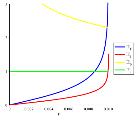
Figure 3. The magnitudes of the periods $\Pi_{c}$, $\Pi_{i}$ and $\Pi_{D}$ along the trajectory from the large volume limit to the field theory limit, for $2\pi^{2}\,u/M_{0}^{2}=-10^{4}$, $c_{0}=1$ and $\xi=10^{-4}$.

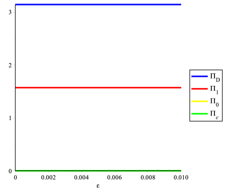
Figure 4. The arguments of the periods $\Pi_{c}$, $\Pi_{i}$ and $\Pi_{D}$ along the trajectory from the large volume limit to the field theory limit, for $2\pi^{2}\,u/M_{0}^{2}=-10^{4}$, $c_{0}=1$ and $\xi=10^{-4}$.

In particular, the phases of the periods $\Pi_{c},\Pi_{0},\Pi_{1},\Pi_{D}$ are almost constant on the trajectory $\gamma_{u}$, and approximatively equal to

(4.11) $$0,{\pi\over 2},{\pi\over 2},{\pi}$$

respectively. Moreover, numerical computations show that the maximum values of

$$|{\rm arg}(\Pi_{D})+{\rm arg}(\Pi_{c})-\pi|,\qquad|{\rm arg}(\Pi_{0})-{\rm arg}(\Pi_{1})|,\qquad|\Pi_{1}|/|\Pi_{0}|$$

over the trajectory can be made arbitrarily small by increasing $|u|/M_{0}^{2}$.

Now, starting at the upper end of the interval, suppose the first wall of marginal stability for a BPS state of charge $\Upsilon_{r,Q}$ encountered along the trajectory $\gamma_{u}$ corresponds to some decomposition

(4.12) $$\Upsilon_{r,Q}=\sum_{i=1}^{n}\Upsilon_{i},\qquad\Upsilon_{i}=r_{i}\Lambda^{1}+s_{i}\Upsilon_{0}+Q_{i}\Upsilon_{1}+q_{i}[{\mathcal{O}}_{p}],\quad 1\leq i\leq n,$$

$r_{i},Q_{i},s_{i},q_{i}\in\mathbb{Z}$ such that the central charge $Z(\Upsilon_{r,Q})$ is aligned with all central charges $Z(\Upsilon_{i})$. Recall that under the current assumptions $\Upsilon_{r,Q}$ must have finite central charge in the field theory limit, hence either $r=0$ and $|Q|=1$ or $r=1$ and $Q\in\mathbb{Z}$ arbitrary.

Then there exist positive real numbers $\lambda_{i}\in\mathbb{R}_{>0}$ such that

$$r_{i}\Pi_{D}+s_{i}\Pi_{0}+Q_{i}\Pi_{1}+q_{i}=\lambda_{i}(r\Pi_{D}+Q\Pi_{1})$$

for all $1\leq i\leq n$ at any point on the marginal stability wall. Given the above behavior of the phases of $\Pi_{c},\Pi_{0},\Pi_{1},\Pi_{D}$ along a path $\gamma_{u}$, by taking $|u|/M_{0}^{2}$ sufficiently large, it follows that

(4.13) $$s_{i}\Pi_{0}+(Q_{i}-\lambda_{i}Q)\Pi_{1}=0,\qquad(r_{i}-\lambda_{i}r)\Pi_{D}+q_{i}=0$$

for all $1\leq i\leq n$ at the intersection point with the wall. Since the ratio $|\Pi_{1}|/|\Pi_{0}|$ can be made arbitrarily small by a suitable choice of $|u|/M_{0}^{2}>>1$, it follows that

(4.14) $$s_{i}=0,\qquad Q_{i}=\lambda_{i}Q$$

for all $1\leq i\leq n$. Since $\lambda_{i}>0$, $n\geq 2$ and $\sum_{i=1}^{n}Q_{i}=Q$, this rules out the case $r=0$, $Q=\pm 1$. Therefore in order for such an intersection point to exist one must have $r=1$ and $Q\in\mathbb{Z}$.

Next we show that if $Q=0$ the BPS degeneracy of the charge $\Upsilon_{r,Q}$ does not jump across a wall of the form (4.12). If $Q=0$, equation (4.14) implies that $Q_{i}=0$ for all $1\leq i\leq n$. The symplectic pairing of any two $K$-theory classes $\Upsilon_{i},\Upsilon_{j}$ with $s_{i}=s_{j}=0$ is

$$\langle\Upsilon_{i},\Upsilon_{j}\rangle=2(r_{j}Q_{i}-r_{i}Q_{j}).$$

Hence if $Q_{i}=Q_{j}=0$ the charges are orthogonal. Since this holds in this case for any pair of charges $\Upsilon_{i},\Upsilon_{j}$, the Kontsevich-Soibelman wallcrossing formula implies that the BPS degeneracy does not jump across such a wall. This holds for refined BPS degeneracies as well.

Finally, suppose $r=1$ and $Q\neq 0$. Then equations (4.13), (4.14) imply

$$(r_{i}Q-Q_{i})\Pi_{D}+q_{i}=0$$

at the intersection point for all $1\leq i\leq n$. However $\Pi_{D}$ is locally a holomorphic function, after choosing appropriate branch cuts. Hence for given $(r,Q_{i},q_{i})$, the equations $(r_{i}Q-Q_{i})\Pi_{D}+q_{i}=0$ can hold at most on a complex codimension one locus in the moduli space. Therefore there will exist a smooth local deformation ${\tilde{\gamma}}_{u}$ of the path $\gamma_{u}$ in an arbitrarily small tubular neighborhood of the marginal stability wall avoiding the subspace $(r_{i}Q-Q_{i})\Pi_{D}+q_{i}=0$, $1\leq i\leq n$. The above argument implies that such a perturbation cannot intersect the wall.

The above argument applies to any marginal stability wall of the form (4.12), with the caveat that the required lower bound on $|u|^{2}/M_{0}^{2}$ will depend on the wall. Therefore, if the number of possible marginal stability walls of the form (4.12) is finite, one can find a uniform lower bound on $|u|^{2}/M_{0}^{2}$ such that the argument applies simultaneously to all the walls. In this case, for sufficiently large $|u|/M_{0}^{2}>>1$, there will exist a smooth small deformation ${\tilde{\gamma}}_{u}$ of the path ${\gamma}_{u}$ such that the BPS degeneracy of charge $\Upsilon_{r,Q}$ is constant along ${\tilde{\gamma}}_{u}$.

Motivated by this example we will formulate next an absence of walls conjecture for all values of $N\geq 2$.

4.3. Limit weak coupling spectrum and absence of walls

Summarizing the facts, there are two distinct scaling limits of Kähler parameters, the field theory limit in Section 2.3, and the large radius limit in Section 4.1. The basic idea of the absence of walls conjecture is that these two limits commute in an appropriate sense, as far as the BPS spectrum is concerned. The goal of this section is to cast this idea in a precise mathematical form.

First we define the limit weak coupling BPS spectrum in gauge theory by analogy with the large radius limit spectrum in string theory. Suppose $a=(a_{i})$ as defined in Section 2.3 is a fixed point on the Coulomb branch within the radius of convergence of the semiclassical expansion such that

$$\qquad{\rm Im}(a_{i})>0,\qquad 1\leq i\leq N-1.$$

In this section the units will be chosen such that $\Lambda=1$, hence the $a_{i}$ are dimensionless. Let $\tau_{0}$, ${\rm Im}(\tau_{0})>0$, be a fixed complex number in the upper half plane. The limit weak coupling spectrum will be defined as the large $\lambda$ limit of the BPS spectrum at points of the form

$$a_{i}(\lambda)={\rm Re}(a_{i})+\lambda\sqrt{-1}{\rm Im}(a_{i}),\qquad\lambda\in\mathbb{R}_{>0},$$

on the Coulomb branch in a gauge theory with tree level coupling

$$\tau_{0}(\lambda)={\rm Re}(\tau_{0})+\lambda\sqrt{-1}{\rm Im}(\tau_{0}).$$

In order to justify the existence of such a limit, note that the leading terms in the large $\lambda$ expansion of the dual periods $a_{i}^{D}$ derived from the prepotential (2.45) are

$$(a_{i}^{D})_{\lambda}= -N{\rm Im}(\tau_{0})\lambda^{2}\sum_{j=1}^{N-1}{\sf C}_{ij}^{-1}{\rm Im}(a_{j})$$

$$\ +N\lambda\sqrt{-1}\big{[}{\rm Re}(\tau_{0})\sum_{j=1}^{N-1}{\sf C}_{ij}^{-1}{\rm Im}(a_{j})+{\rm Im}(\tau_{0})\sum_{j=1}^{N-1}{\sf C}_{ij}^{-1}{\rm Re}(a_{j})\big{]}+\cdots$$

The subleading terms are of order $\lambda\ln\lambda$ for the real part and $\ln\lambda$ for the imaginary part. The leading terms in the expansion of the stability parameters (2.51) are

(4.15) $$z_{i,\lambda} =\big{(}\sum_{j=1}^{N-1}{\sf C}_{ij}(a_{j}^{D})_{\lambda}-\lambda(i+1)\sqrt{-1}{\rm Im}(a_{i})\big{)}$$

$$w_{i,\lambda} =\big{(}-\sum_{j=1}^{N-1}{\sf C}_{ij}(a_{j}^{D})_{\lambda}+\lambda i\sqrt{-1}{\rm Im}(a_{i})\big{)}$$

Equations (4.15) determine a linear function on the charge lattice $\Gamma\simeq K^{0}({\mathcal{G}})$ whose $\lambda$-dependence is of the form:

$$Z_{(\tau_{0},a,\lambda)}=\lambda^{2}Z^{(2)}_{(\tau_{0},a)}+\lambda\sqrt{-1}Z^{(1)}_{(\tau_{0},a)}:\Gamma\to\mathbb{C}.$$

Recall that ${\mathcal{G}}\subset D^{b}(X_{N})$ is the triangulated subcategory spanned by the fractional branes $(P_{i},Q_{i})$, $1\leq i\leq N-1$. The abelian category of $(Q,W)$-modules is the heart of a $t$-structure on ${\mathcal{G}}$ and its $K$-theory is isomorphic to $\Gamma$. The same will hold for any quiver with potential $(Q^{\prime},W^{\prime})$ related to $(Q,W)$ by a finite sequence of mutations. Namely the $K$-theory of the abelian category of $(Q^{\prime},W^{\prime})$-modules will be isomorphic to $\Gamma$. Let $\Gamma_{(Q^{\prime},W^{\prime})}\subset\Gamma$ be the cone spanned by the simple representations of $(Q^{\prime},W^{\prime})$ in the charge lattice. In order to define the limit weak coupling spectrum we will make the following assumption:

For sufficiently generic $(\tau_{0},a)$ there exists $\lambda_{0}>0$, depending on $(\tau_{0},a)$, a quiver with potential $(Q,W)_{(\tau_{0},a)}$, mutation equivalent to $(Q,W)$, and $\sigma\in\{-1,1\}$ such that $\sigma Z^{(1)}_{(\tau_{0},a,\lambda)}$ takes positive values on $\Gamma_{(Q,W)_{(\tau_{0},a)}}\setminus\{0\}$.

Granting this assumption, for any sufficiently generic $(\tau_{0},a)$ there is a slope function

(4.16) $$\mu_{(\tau_{0},a)}:\Gamma\to\mathbb{C},\qquad\mu_{(\tau_{0},a)}(\gamma)=-{Z^{(2)}_{(\tau_{0},a)}(\gamma)\over Z^{(1)}_{(\tau_{0},a)}(\gamma)}=-\sigma{Z^{(2)}_{(\tau_{0},a)}(\gamma)\over\big{|}Z^{(1)}_{(\tau_{0},a)}(\gamma)\big{|}}$$

Since the denominator takes positive values on the effective cone, this yields a well-defined stability condition for $(Q^{\prime},W^{\prime})$-modules. A representation $\rho$ of the quiver with potential $(Q^{\prime},W^{\prime})$ with dimension vector $\gamma$ will be called $\mu_{(\tau_{0},a)}$-(semi)stable if

$$\mu_{(\tau_{0},a)}(\gamma^{\prime})\ (\leq)\ \mu_{(\tau_{0},a)}(\gamma)$$

for any nontrivial proper subrepresentation $0\subset\rho^{\prime}\subset\rho$ with dimension vector $\gamma^{\prime}$. The moduli space of $\mu_{(\tau_{0},a)}$-semistable representations of $(Q^{\prime},W^{\prime})$ with fixed charge $\gamma$ will be denoted by ${\mathcal{M}}^{gauge}_{(\tau_{0},a)}(\gamma)$. This moduli space defines the limit weak coupling spectrum. More precisely, the limit protected spin characters $\Omega_{(\tau_{0},a)}^{gauge}(\gamma;y)$ are identified as explained in Section 2.5 with refined counting invariants of these moduli spaces.

As a concrete example, note that

$$z_{i,\lambda} =\lambda^{2}z^{(2)}_{i}+\lambda\sqrt{-1}z^{(1)}_{i}$$

$$w_{i,\lambda} =\lambda^{2}w^{(2)}_{i}+\lambda\sqrt{-1}w^{(1)}_{i}$$

where

(4.17) $$z^{(2)}_{i} =-N{\rm Im}(\tau_{0}){\rm Im}(a_{i})$$

$$z^{(1)}_{i} =N{\rm Re}(\tau_{0}){\rm Im}(a_{i})+N{\rm Im}(\tau_{0}){\rm Re}(a_{i})-(i+1){\rm Im}(a_{i})$$

$$w^{(2)}_{i} =N{\rm Im}(\tau_{0}){\rm Im}(a_{i})$$

$$w^{(1)}_{i} =-N{\rm Re}(\tau_{0}){\rm Im}(a_{i})-N{\rm Im}(\tau_{0}){\rm Re}(a_{i})+i{\rm Im}(a_{i})$$

for $1\leq i\leq N-1$. Next note that

$$z^{(1)}_{i}<0,\qquad w^{(1)}_{i}<0,\qquad 1\leq i\leq N-1$$

if the inequalities

(4.18) $$0<N{\rm Re}(\tau_{0}){\rm Im}(a_{i})+{\rm Im}(\tau_{0}){\rm Re}(a_{i})-i{\rm Im}(a_{i})<{\rm Im}(a_{i})$$

hold for all $1\leq i\leq N-1$. Therefore the main assumption formulated above holds in this case with $\sigma=-1$ if $a$ belongs to the wedge (4.18).

The absence of walls conjecture will be formulated as an identification between the limit weak coupling spectrum defined above and the limit large radius defined in Section 4.1 spectrum in a specific $(\omega,B)$-stability chamber to be defined below.

Recall that the complex Kähler class was written as

$$B+\sqrt{-1}\omega=(b_{0}+\sqrt{-1}t_{0})H+\sum_{i=1}^{N-1}(b_{i}+\sqrt{-1}t_{i})D_{i}$$

where $s_{i}=b_{i}+\sqrt{-1}t_{i}$, $i=0,\ldots,N-1$, are the periods of $B+\sqrt{-1}\omega$ on the Mori cone generators $\Sigma_{0},C_{i}$, $i=1,\ldots,N-1$. The field theory limit was defined in Section 2.3 by setting

(4.19) $$b_{0}+t_{0}\sqrt{-1} ={-N\over\pi}(c_{0}+\ln\epsilon)\sqrt{-1},$$

$$b_{i}+\sqrt{-1}t_{i} =\epsilon{a_{i}\over M_{0}}$$

for $1\leq i\leq N-1$, with $0<\epsilon<e^{-c_{0}}$, and keeping the leading terms of the central charge (4.1) in the small $\epsilon$ expansion. Since $\Lambda$ has been set to $1$, equation (2.36) yields

$$M_{0}=2\pi\left(2{e^{c_{0}}}\right)^{-N/(N-1)}$$

The parameter $c_{0}>0$ is related to the field theory coupling constant $\tau_{0}$ by the equation

(4.20) $$\tau_{0}={1\over 2}+{\sqrt{-1}\over\pi}\left({c_{0}+N\ln 2\over N-1}-{3\over 2}\right)$$

obtained from (2.45). This has led to the conclusion that finite mass BPS states in this limit must be objects of the subcategory ${\mathcal{G}}\subset D^{b}(X_{N})$ generated by the fractional branes $(P_{i},Q_{i})_{1\leq i\leq N-1}$.

Now note that ${\mathcal{G}}$ is identified with the subcategory of $D^{b}_{cpt}(X_{N})$ defined by the orthogonality conditions

(4.21) $${\rm RHom}_{X_{N}}({\mathcal{O}}_{X_{N}}(aH),F)=0,\qquad a=0,1.$$

This follows from the expression (2.9) of the tilting functor:

$$F\mapsto{\rm RHom}_{X_{N}}(T,F),\qquad T=\bigoplus_{i=1}^{N}({\mathcal{L}}_{i}\oplus{\mathcal{M}}_{i}).$$

For each $1\leq i\leq N$, the complexes of vector spaces ${\rm RHom}_{X_{N}}({\mathcal{L}}_{i},F)$, ${\rm RHom}_{X_{N}}({\mathcal{M}}_{i},F)$ are quasi-isomorphic to

$$\bigoplus_{k\in\mathbb{Z}}H^{k}(X_{N},{\mathcal{L}}_{i}^{-1}\otimes_{X_{N}}F)[-k],\qquad\bigoplus_{k\in\mathbb{Z}}H^{k}(X_{N},{\mathcal{M}}_{i}^{-1}\otimes_{X_{N}}F)[-k].$$

Then ${\rm RHom}_{X_{N}}(T,F)$ is a complex $\rho_{F}$ of $({\mathcal{Q}},{\mathcal{W}})$-modules such that the $k$-th term of the complex $\rho_{F}^{k}$ has underlying vector spaces

$$H^{k}(X_{N},{\mathcal{L}}_{i}^{-1}\otimes_{X_{N}}F),\qquad H^{k}(X_{N},{\mathcal{M}}_{i}^{-1}\otimes_{X_{N}}F)$$

respectively at the nodes $p_{i},q_{i}$, $1\leq i\leq N$. Therefore, for a sheaf $F$ satisfying conditions (4.21), all $\rho_{F}^{k}$ have trivial vector spaces at the nodes $(p_{N},q_{N})$. This implies that $\rho_{F}$ belongs to the subcategory spanned by the fractional branes $(P_{i},Q_{i})$, $1\leq i\leq N-1$.

Next note that any compactly supported sheaf $F$ satisfying conditions (4.21) must have numerical invariants

(4.22) $${\mathrm{ch}}_{0}(F)=0,\qquad{\mathrm{ch}}_{1}(F)=\sum_{i=1}^{N-1}m_{i}S_{i},\qquad{\mathrm{ch}}_{2}(F)=\sum_{i=1}^{N-1}n_{i}C_{i},\qquad\chi(F)=0,$$

where $m_{i},n_{i},\in\mathbb{Z}$ with $m_{i}\geq 0$, $i=1,\ldots,N-1$. If $F$ has two dimensional support, ${\mathrm{ch}}_{1}(F)\neq 0$, hence the $m_{i}$, $i=1,\ldots,N-1$ cannot all be zero. In comparison with (4.5), note that the invariants $p,n$ in (4.5) must vanish.

Finally, note that the following result holds by a standard boundedness argument which will be omitted.

For fixed $(c_{0},a_{i})$ and a fixed effective $K$-theory class $\gamma\in K_{0}({\mathcal{G}})$ there exists $0<\epsilon_{0}<e^{-c_{0}}$ depending on $(c_{0},a_{i};\gamma)$ such that the moduli space of $(\omega,B)$-semistable sheaves $F$ with $K$-theory class $[F]=\gamma$ is constant (as a scheme) and independent of $\epsilon$, for $0<\epsilon<\epsilon_{0}$.

Let ${\mathcal{M}}^{string}_{(\tau_{0},a)}(\gamma)$ denote the small $\epsilon$ limit of the moduli space of $(\omega,B)$-semistable sheaves with $K$-theory class $\gamma=[F]$. For classes of the form $\gamma=-[F]$, with a compactly supported sheaf, let ${\mathcal{M}}^{string}_{(\tau_{0},a)}(\gamma)={\mathcal{M}}^{string}_{(\tau_{0},a)}(-\gamma)$. If $\gamma$ is not of the form $\pm[F]$ with $F$ a sheaf with compact support, by convention, ${\mathcal{M}}^{string}_{(\tau_{0},a)}(\gamma)$ will be empty. Similarly, let $\Omega_{(\tau_{0},a)}^{string}(\gamma;y)$, denote the small $\epsilon$ limit of the corresponding protected spin characters. We extend the assignment

$$\gamma\mapsto\Omega_{(\tau_{0},a)}^{string}(\gamma;y)$$

to a function on the whole $K$-theory lattice $K^{0}({\mathcal{G}})$, setting

$$\Omega_{(\tau_{0},a)}^{string}(\gamma;y)=\left\{\begin{array}[]{ll}\Omega_{(\tau_{0},a)}^{string}(\gamma;y),&{\rm if}\ \gamma=[F]\ {\rm for\ some\ compactly\ supported\ sheaf}\ F,\\ &\\ \Omega_{(\tau_{0},a)}^{string}(-\gamma;y),&{\rm if}\ \gamma=-[F]\ {\rm for\ some\ compactly\ supported\ sheaf}\ F,\\ &\\ 0,&{\rm otherwise}.\\ \end{array}\right.$$

Finally, the absence of walls conjecture states that:

For a given charge vector $\gamma\in\Gamma$, there is a one-to-one correspondence

(4.23) $${\mathcal{P}}_{\gamma}:\big{\{}{\mathcal{C}}^{gauge}(\gamma)\}\longrightarrow\big{\{}{\mathcal{C}}^{string}(\gamma)\big{\}}$$

between quiver stability chambers ${\mathcal{C}}^{gauge}(\gamma)$ with respect to $\mu_{(\tau_{0},a)}$-stability and geometric stability chambers ${\mathcal{C}}^{string}(\gamma)$ with respect to small $\epsilon$ $(\omega,B)$-stability such that there is an isomorphism of moduli spaces

(4.24) $${\mathcal{M}}^{gauge}_{{\mathcal{C}}^{gauge}(\gamma)}(\gamma)\simeq{\mathcal{M}}^{string}_{{\mathcal{P}}_{\gamma}({\mathcal{C}}^{gauge}(\gamma))}(\gamma)$$

and relation of the form

(4.25) $$\Omega^{gauge}_{{\mathcal{C}}^{gauge}(\gamma)}(\gamma;y)=\Omega_{{\mathcal{P}}_{\gamma}({\mathcal{C}}^{gauge}(\gamma))}^{string}(\gamma;y)$$

for any chamber ${\mathcal{C}}^{gauge}(\gamma)$.

Recall that the stability chambers ${\mathcal{C}}^{gauge}(\gamma)$ are subsets of the universal cover of the Coulomb branch. Similarly, the chambers ${\mathcal{C}}^{string}(\gamma)$ are subsets of the universal cover of the complex Kähler moduli space, which is parameterized by $(\omega,B)$ in a neighborhood of the large radius limit.

As a first consistency check of this conjecture, note that a priori the limit moduli spaces ${\mathcal{M}}^{string}_{(\tau_{0},a)}(\gamma)$ might include $(\omega,B)$-semistable sheaves $F$ which do not belong to the subcategory ${\mathcal{G}}$. The orthogonality conditions (4.21) are equivalent to the vanishing results

(4.26) $$H^{k}(X_{N},F(-aH))=0,\qquad k=0,1,2,\qquad a=0,1.$$

Any semistable sheaf $F$ with $K$-theory class $[F]\in K^{0}({\mathcal{G}})$ satisfies

(4.27) $$0=\chi(F(-aH))=\sum_{k=0}^{2}(-1)^{k}{\rm dim}H^{k}(X_{N},F(-aH)),$$

where the first equality follows because $K^{0}({\mathcal{G}})$ is generated by the $K$-theory classes $[P_{i}],[Q_{i}]$, $1\leq i\leq N-1$, and $\chi(P_{i})=\chi(Q_{i})=0$, $1\leq i\leq N-1$. (See equation (2.15) above.) However, the dimensions of the cohomology groups can be nontrivial. In fact, the dimensions of these groups are expected to jump as $F$ moves in the moduli space. Hence a priori the orthogonality conditions (4.21) are not guaranteed to hold throughout the moduli space even for classes $\gamma\in K^{0}({\mathcal{G}})$. The following result proves that they do in fact hold at all points of the limit moduli spaces ${\mathcal{M}}^{string}_{(\tau_{0},a)}(\gamma)$.

For fixed parameters $a_{i}$, $i=0,\ldots,N-1$ satisfying

(4.28) $$\qquad{\rm Re}(a_{i})\neq 0,\qquad{\rm Im}(a_{i})>0,\qquad i=1,\ldots,N-1$$

and fixed $m_{i},n_{i}\in\mathbb{Z}$, there exists $0<\epsilon_{1}<1$ such that for all $0<\epsilon<\epsilon_{1}$, any $(\omega,B)$-semistable sheaf $F$ with numerical invariants (4.22) satisfies conditions (4.21). In particular all such objects belong to the subcategory ${\mathcal{G}}\subset D^{b}(X_{N})$.

In order to prove this statement, recall that any pure dimension two $(\omega,B)$-semistable sheaf $F$ with compact support must be scheme theoretically supported on $S$. This implies

$$H^{k}(X_{N},F(-aH))\simeq H^{k}(S,F(-aH))$$

for all $k,a$. Therefore the required vanishing results for $k=0$ follow if one can prove that

$${\rm Hom}_{S}({\mathcal{O}}_{S}(aH),F)\simeq{\rm Hom}_{X_{N}}({\mathcal{O}}_{S}(aH),F),$$

with $a=0,1$, vanishes. Moreover note that Serre duality holds on $S$ since $S\subset X_{N}$ is a divisor, and the dualizing sheaf is given by the adjunction formula

$$\omega_{S}\simeq{\mathcal{O}}_{S}(S).$$

Hence

$$H^{2}(S,F(-aH)) \simeq{\rm Ext}^{2}_{S}({\mathcal{O}}_{S}(aH),F)\simeq{\rm Ext}^{0}_{S}(F,{\mathcal{O}}_{S}(aH+S))^{\vee}$$

$$\simeq{\rm Ext}^{0}_{X_{N}}(F,{\mathcal{O}}_{S}(aH+S))^{\vee},$$

where the last isomorphism holds because both $F$ and ${\mathcal{O}}_{S}(aH+S)$ are extensions by zero of sheaves on $S$. Then the vanishing results for $k=2$ also follow if one can prove that

$${\rm Hom}_{X_{N}}(F,{\mathcal{O}}_{S}(aH+S))=0,\qquad a=0,1.$$

If the vanishing results (4.26) hold for $k=0,2$, then equation (4.27) implies that they must also hold for $k=1$.

In conclusion it suffices to prove that

(4.29) $${\rm Hom}_{X_{N}}({\mathcal{O}}_{S}(aH),F)=0,\qquad{\rm Hom}_{X_{N}}(F,{\mathcal{O}}_{S}(S+aH))=0,\qquad a=0,1,$$

for any $(\omega,B)$-semistable sheaf $F$, provided that $\epsilon>0$ is sufficiently small.

To explain the main idea of the proof, note that given any nontrivial morphism $\phi:{\mathcal{O}}_{S}(aH)\to F$, the image subsheaf ${\rm Im}(\phi)\subset F$ must satisfy the stability condition

$$\mu_{(\omega,B)}({\rm Im}(\phi))\leq\mu_{(\omega,B)}(F).$$

At the same time ${\rm Im}(\phi)$ is a nontrivial quotient of ${\mathcal{O}}_{S}(aH)$. Below we will show that for sufficiently small $\epsilon>0$ any nontrivial quotient of ${\mathcal{O}}_{S}(aH)$ violates the above slope inequality. This implies that there cannot exist nontrivial morphisms $\phi:{\mathcal{O}}_{S}(aH)\to F$. The argument for the second vanishing result in (4.29) is similar. Given any nontrivial morphism $\psi:F\to{\mathcal{O}}_{S}(aH+S)$, its image ${\rm Im}(\psi)$ is simultaneously a quotient of $F$ and a subsheaf of ${\mathcal{O}}_{S}(aH+S)$. In particular it must satisfy

$$\mu_{(\omega,B)}({\rm Im}(\psi))\geq\mu_{(\omega,B)}(F).$$

We will show below that this yields a contradiction for sufficiently small $\epsilon>0$.

To this end, using equations (2.32),(4.2), (4.19) and (4.22), the leading term of the slope $\mu_{(\omega,B)}(F)$ in the small $\epsilon$ expansion is

(4.30) $$\mu_{(\omega,B)}(F)\sim-{\sum_{i=1}^{N-1}m_{i}{\rm Re}(a_{i})\over\sum_{i=1}^{N-1}m_{i}{\rm Im}(a_{i})}.$$

Next note that

$${\mathrm{ch}}_{1}({\mathcal{O}}_{S}(aH))=\sum_{i=1}^{N-1}S_{i},\qquad{\mathrm{ch}}_{2}({\mathcal{O}}_{S}(aH))=\Sigma_{0}+\sum_{i=1}^{N-1}(i+1+a)C_{i}$$

$${\mathrm{ch}}_{1}({\mathcal{O}}_{S}(S+aH))=\sum_{i=1}^{N-1}S_{i},\qquad{\mathrm{ch}}_{2}({\mathcal{O}}_{S}(S+aH))=-\Sigma_{0}-\sum_{i=1}^{N-1}(i+1-a)C_{i}.$$

Moreover any pure dimension two quotient ${\mathcal{O}}_{S}\twoheadrightarrow G$ must be the structure sheaf, $G\simeq{\mathcal{O}}_{Z}$, of a closed subscheme $Z\subseteq S$. Since $S$ is a reduced divisor defined by the equation

$$\prod_{i=1}^{N-1}x_{i}=0$$

any such subscheme will be a reduced divisor $S_{j_{1},\ldots,j_{k}}$ defined by an equation of the form

$$\prod_{j=1}^{k}x_{i_{j}}=0$$

for some subset $\{j_{1},\ldots,j_{k}\}\subset{1,\ldots,N-1}$. A straightforward computation shows that

$${\mathrm{ch}}_{1}({\mathcal{O}}_{S_{j_{1},\ldots,j_{k}}})=\sum_{j=1}^{k}S_{i_{j}},$$

and

$${\mathrm{ch}}_{2}({\mathcal{O}}_{S_{j_{1},\ldots,j_{k}}})=p(j_{1},\ldots,j_{k})\Sigma_{0}+\sum_{i=1}^{N-1}n_{i}(j_{1},\ldots,j_{k})C_{i}$$

where $p(j_{1},\ldots,j_{k})$ is the number of connected components of $S_{j_{1},\ldots,j_{k}}$.

In order to prove the last statement, note that

$${\mathrm{ch}}({\mathcal{O}}_{S_{j_{1},\ldots,j_{k}}})=1-e^{-S_{j_{1},\ldots,j_{k}}}$$

since $S_{j_{1},\ldots,j_{k}}$ is a divisor. Hence

$${\mathrm{ch}}_{2}({\mathcal{O}}_{S_{j_{1},\ldots,j_{k}}})=-{1\over 2}\big{(}{S_{j_{1},\ldots,j_{k}}}\big{)}^{2}=-{1\over 2}\sum\big{(}{S^{c}_{j_{1},\ldots,j_{k}}}\big{)}^{2}$$

where the sum is over the connected components of ${S_{j_{1},\ldots,j_{k}}}$. Therefore it suffices to compute $\big{(}{S_{j_{1},\ldots,j_{k}}}\big{)}^{2}$ assuming $S_{j_{1},\ldots,j_{k}}$ is connected. This implies that $j_{1},\ldots,j_{k}$ must be consecutive integers in the set $\{1,\ldots,N-1\}$ up to a permutation. Without loss of generality one can assume $j_{i+1}=j_{i}+1$ for all $1\leq i\leq k-1$. Then, using the linear relation

$${S_{j_{1},\ldots,j_{k}}}=\sum_{j=j_{1}}^{j_{k}}S_{j},$$

and the intersection products

$$(S_{i}\cdot S_{j})_{X_{N}}=\left\{\begin{array}[]{ll}\Sigma_{i},&{\rm for}\ j=i+1\\ \Sigma_{j},&{\rm for}\ i=j+1\\ -\Sigma_{i-1}-\Sigma_{i}-2C_{i},&{\rm for}\ i=j,\\ 0,&{\rm otherwise}\\ \end{array}\right.$$

one obtains

$$\big{(}{S_{j_{1},\ldots,j_{k}}}\big{)}^{2} =\sum_{j=j_{1}}^{j_{k}}(S_{j})^{2}+2\sum_{j=j_{1}+1}^{j_{k}-1}(S_{j}\cdot S_{j+1})$$

$$=-\sum_{j=j_{1}}^{j_{k}}(\Sigma_{j-1}+\Sigma_{j}+2C_{j})+2\sum_{j=j_{1}+1}^{j_{k}-1}\Sigma_{j}$$

By convention, the sum from $j_{1}+1$ to $j_{k}-1$ in the above equations is 0 if $j_{1}+1>j_{k}-1$. Using the relations $\Sigma_{j}=\Sigma_{j-1}+2jC_{j}$ recursively, it follows that

$$\big{(}{S_{j_{1},\ldots,j_{k}}}\big{)}^{2}=-2\Sigma_{0}+\cdots$$

where $\cdots$ is a linear combination of fiber classes $C_{j}$. This proves the claim.

The coefficients $n_{i}(j_{1},\ldots,j_{k})$ can be computed but explicit expressions are not needed in the following. The essential fact is that $p(j_{1},\ldots,j_{k})\geq 1$ for any nonempty subset $\{j_{1},\ldots,j_{k}\}$. Twisting by ${\mathcal{O}}_{X_{N}}(S)$, it follows that

$${\mathrm{ch}}_{1}({\mathcal{O}}_{S_{j_{1},\ldots,j_{k}}}(S))=\sum_{j=1}^{k}S_{i_{j}},$$

and

$${\mathrm{ch}}_{2}({\mathcal{O}}_{S_{j_{1},\ldots,j_{k}}}(S)) ={\mathrm{ch}}_{2}({\mathcal{O}}_{S_{j_{1},\ldots,j_{k}}})+(S\cdot S_{j_{1},\ldots,j_{k}})_{X_{N}}$$

$$=({\tilde{p}}(j_{1},\ldots,j_{k})-p(j_{1},\ldots,j_{k}))\Sigma_{0}+\sum_{i=1}^{N-1}{\tilde{n}}_{i}(j_{1},\ldots,j_{k})C_{i}$$

where ${\tilde{p}}_{j_{1}\ldots,j_{k}}$ is the number of connected components of the intersection $S_{j_{1},\ldots,j_{k}}\cap\left(S\setminus S_{j_{1},\ldots,j_{k}}\right)$. Since $S$ is a linear chain of divisors, it is straightforward to check that

$${\tilde{p}}(j_{1},\ldots,j_{k})-p(j_{1},\ldots,j_{k})\geq 0$$

This implies that the kernel $K(j_{1},\ldots j_{k})={\rm Ker}({\mathcal{O}}_{S}(S)\twoheadrightarrow{\mathcal{O}}_{S_{j_{1},\ldots,j_{k}}}(S))$ has second Chern character

$${\mathrm{ch}}_{2}(K(j_{1},\ldots,j_{k}))=q(j_{1},\ldots,j_{k})\Sigma_{0}-\sum_{i=1}^{N-1}(i+1-{\tilde{n}}_{i}(j_{1},\ldots,j_{k}))C_{i}$$

with $q(j_{1},\ldots,j_{k})<0$. In conclusion any quotient of ${\mathcal{O}}_{S}(aH)$ must be of the form ${\mathcal{O}}_{S_{j_{1},\ldots,j_{k}}}(aH)$ and the leading term of its $(\omega,B)$-slope is

(4.31) $$\mu_{(\omega,B)}({\mathcal{O}}_{S_{j_{1},\ldots,j_{k}}}(aH))\sim{M_{0}\over\epsilon}{p(j_{1},\ldots,j_{k})\over\sum_{j=1}^{k}{\rm Im}(a_{j_{k}})}\qquad p(j_{1},\ldots,j_{k})\geq 1.$$

Any nontrivial subsheaf of ${\mathcal{O}}_{S}(S+aH)$ must be of the form $K(j_{1},\ldots,j_{k})(aH)$ and the leading term of its $(\omega,B)$-slope is

(4.32) $$\mu_{(\omega,B)}(K({j_{1},\ldots,j_{k}})(aH))\sim{M_{0}\over\epsilon}{q(j_{1},\ldots,j_{k})\over\sum_{j=1}^{k}{\rm Im}(a_{j_{k}})},\qquad q(j_{1},\ldots,j_{k})\leq-1.$$

Therefore

$$\mu_{(\omega,B)}(K({j_{1},\ldots,j_{k}})(aH))<\mu_{(\omega,B)}(F)<\mu_{(\omega,B)}({\mathcal{O}}_{S_{j_{1},\ldots,j_{k}}}(aH))$$

for sufficiently small $0<\epsilon<<1$. Moreover, given the numerical invariants (4.22), $F$ cannot be isomorphic to a quotient of ${\mathcal{O}}_{S}(aH)$ or to a subobject of ${\mathcal{O}}_{S}(S+aH)$. As explained below equation (4.29), the above inequalities lead to a contradiction for sufficiently small $0<\epsilon<\epsilon_{0}$. Since there are finitely many subsets $\{j_{1},\ldots,j_{k}\}\subset\{1,\ldots,N-1\}$, the upper bound $\epsilon_{0}$ depends only on $a_{i}$, $m_{i}$, $i=1,\ldots,N-1$.

Since the presentation has been so far fairly general, it may be helpful to study some examples in detail. The simplest example is $N=2$, which was discussed in detail in Section 4.2. For $N=3$, the moduli spaces of stable sheaves in the field theory region are very complicated for arbitrary numerical invariants $(m_{1},m_{2})$. However, the case $(m_{1},m_{2})=(1,1)$ is tractable and will be treated next.

4.4. $SU(3)$ spectrum with magnetic charges $(1,1)$

Using the results of Sections 4.1 and 4.3, any $(\omega,B)$-semistable sheaf $F$ must be scheme theoretically supported on the reduced divisor $S=S_{1}+S_{2}$ and have numerical invariants

$${\mathrm{ch}}_{1}(F)=m_{1}S_{1}+m_{2}S_{2},\qquad{\mathrm{ch}}_{2}(F)=n_{1}C_{1}+n_{2}C_{2},\qquad\chi(F)=0.$$

The $K$-theory class of such a sheaf will be denoted by $\gamma(m_{1},m_{2},n_{1},n_{2})\in\Gamma\simeq K^{0}({\mathcal{G}})$. The symplectic pairing of two $K$-theory classes $\gamma(m_{1},m_{2},n_{1},n_{2})$, $\gamma(m^{\prime}_{1},m^{\prime}_{2},n^{\prime}_{1},n^{\prime}_{2})$ is given by

(4.33) $$\langle\gamma(m_{1},m_{2},n_{1},n_{2}),\gamma(m^{\prime}_{1},m^{\prime}_{2},n^{\prime}_{1},n^{\prime}_{2})\rangle=$$

$$m_{1}^{\prime}(n_{2}-2n_{1})+m_{2}^{\prime}(n_{1}-2n_{2})-m_{1}(n^{\prime}_{2}-2n^{\prime}_{1})-m_{2}(n^{\prime}_{1}-2n_{2}^{\prime}).$$

Suppose $F$ is such a sheaf with $(m_{1},m_{2})\neq(0,0)$. Then there is an exact sequence

(4.34) $$0\to F_{1}\to F\to F_{2}\to 0$$

uniquely determined by $F$, with $F_{1},F_{2}$ pure dimension two sheaves with scheme theoretic support on $S_{1},S_{2}$ respectively. Recall that $S_{1}\simeq{\mathbb{F}}_{2}$, $S_{2}\simeq{\mathbb{F}}_{4}$. Note that $F_{2}$ is the quotient of $F\otimes_{X_{3}}{\mathcal{O}}_{S_{2}}$ by its maximal dimension subsheaf of dimension at most one, and $F_{1}$ the kernel of the resulting projection $F\twoheadrightarrow F_{2}$. Recall that $\otimes_{X_{3}}$ denotes the tensor product of ${\mathcal{O}}_{X_{3}}$-modules. Obviously,

$${\mathrm{ch}}_{1}(F_{1})=m_{1}S_{1},\qquad{\mathrm{ch}}_{1}(F_{2})=m_{2}S_{2},$$

and

$${\mathrm{ch}}_{2}(F_{1})=-p\Sigma_{1}+n_{1}C_{1},\qquad{\mathrm{ch}}_{2}(F_{2})=p\Sigma_{1}+n_{2}C_{2}$$

with $p\in\mathbb{Z}$.

By analogy with [51, Lemma 2.6], the adjunction formula yields an isomorphism

(4.35) $${\rm Ext}^{1}_{X_{3}}(F_{2},F_{1})\simeq{\rm Hom}_{S_{2}}(F_{2},F_{1}\otimes_{X_{3}}{\mathcal{O}}_{S_{2}}(S_{2})).$$

Therefore there is a one to one correspondence between extension classes $e\in{\rm Ext}^{1}_{X_{3}}(F_{2},F_{1})$ and morphisms $\phi_{e}:F_{2}\to F_{1}\otimes_{X_{3}}{\mathcal{O}}_{S_{2}}(S_{2})$. Moreover, this correspondence is functorial. This implies that given any subsheaf $F_{2}^{\prime}\subseteq F_{2}$, the class $e$ is in the kernel of the natural map

$${\rm Ext}^{1}_{X_{3}}(F_{2},F_{1})\to{\rm Ext}^{1}_{X_{3}}(F^{\prime}_{2},F_{1})$$

if and only if $F_{2}^{\prime}\subseteq{\rm Ker}(\phi_{e})$. In particular there is a commutative diagram with exact rows and columns

(4.36)

where ${\widetilde{F}}_{2}={\rm Ker}(\phi_{e})$ and $I={\rm Im}(\phi_{e})$. A slightly more involved argument analogous to [51, Lemma 2.8] shows that ${\widetilde{F}}_{1}$ must be pure of dimension two. Since $I$ is a subsheaf of $F_{1}\otimes_{X_{3}}{\mathcal{O}}_{S_{2}}(S_{2})$, which is dimension one, supported on $\Sigma_{1}$,

$${\mathrm{ch}}_{2}(I)=q\Sigma_{1}$$

for some $q\in\mathbb{Z}$, $0\leq q\leq m_{1}$. This implies that

$${\mathrm{ch}}_{2}({\widetilde{F}}_{1})=(q-p)\Sigma_{1}+n_{1}C_{1},\qquad{\mathrm{ch}}_{2}({\widetilde{F}}_{2})=(p-q)\Sigma_{1}+n_{2}C_{2}.$$

For future reference note that completely analogous considerations apply to the middle vertical column in diagram (4.36). Namely there is an isomorphism

(4.37) $${\rm Ext}^{1}_{X_{3}}({\widetilde{F}}_{1},{\widetilde{F}}_{2})\simeq{\rm Hom}_{S_{1}}({\widetilde{F}}_{1},{\widetilde{F}}_{2}\otimes_{X_{3}}{\mathcal{O}}_{S_{1}}(S_{1})).$$

Hence the associated extension class ${\widetilde{e}}$ corresponds to a morphism $\phi_{\widetilde{e}}:{\widetilde{F}}_{2}\to{\widetilde{F}}_{1}\otimes_{X_{3}}{\mathcal{O}}_{S_{1}}(S_{1})$ whose image will be denoted by ${\widetilde{I}}$. Then a standard diagram chasing argument using the snake lemma proves that ${\widetilde{I}}\simeq I$.

Next recall that in the field theory limit

(4.38) $$b_{0}+t_{0}\sqrt{-1}={-3\over\pi}(c_{0}+\ln(\epsilon/2))\sqrt{-1},\qquad b_{i}+\sqrt{-1}t_{i}=\epsilon{a_{i}\over M_{0}},\qquad i=1,2,$$

with $0<\epsilon<e^{-c_{0}}$, and

$$M_{0}=2\pi\left(2{e^{c_{0}}}\right)^{-3/2}$$

since $\Lambda$ has been set to $1$. Moreover, $c_{0}$ is related to the field theory coupling constant $\tau_{0}$ by

$$\tau_{0}={1\over 2}+{\sqrt{-1}\over\pi}\left({c_{0}+3\ln 2\over 2}-{3\over 2}\right).$$

Note that $t_{i}>0$, hence ${\rm Im}(a_{i})>0$, for $i=1,2$. The coupling constant $\tau_{0}$ must belong to the upper half-plane, hence

$$c_{0}>3(1-\ln 2).$$

In addition, we will also work in the wedge (4.18) on the Coulomb branch, which specializes to

(4.39) $$\left(i-{3\over 2}\right){{\rm Im}(a_{i})\over{\rm Im}(\tau_{0})}<{{\rm Re}(a_{i})}<\left(i-{1\over 2}\right){{\rm Im}(a_{i})\over{\rm Im}(\tau_{0})},\qquad i=1,2.$$

The $(\omega,B)$-slopes have a small $\epsilon$ expansion of the form

$$\mu_{(\omega,B)}(F_{1})\sim -{p\over\epsilon}{M_{0}\over m_{1}{\rm Im}(a_{1})}-{{\rm Re}(a_{1})\over{\rm Im}(a_{1})},\qquad\mu_{(\omega,B)}({\widetilde{F}}_{2})\sim{(p-q)\over\epsilon}{M_{0}\over m_{2}{\rm Im}(a_{2})}-{{\rm Re}(a_{2})\over{\rm Im}(a_{2})},$$

$$\qquad\mu_{(\omega,B)}(F)\sim-{m_{1}{\rm Re}(a_{1})+m_{2}{\rm Re}(a_{2})\over m_{1}{\rm Im}(a_{1})+m_{2}{\rm Im}(a_{2})}.$$

Then, taking the small $\epsilon$ limit with $(\tau_{0},a_{i})$ fixed the necessary semistability conditions

(4.40) $$\mu_{(\omega,B)}(F_{1})\leq\mu_{(\omega,B)}(F),\qquad\mu_{(\omega,B)}({\widetilde{F}}_{2})\leq\mu_{(\omega,B)}(F)$$

yield

$$0\leq p\leq q.$$

By construction we also have $q\leq m_{1}$ as explained above. Therefore $p,q$ must satisfy the constraints

(4.41) $$0\leq p\leq q\leq m_{1}$$

This is as far as we can go for arbitrary magnetic charges $(m_{1},m_{2})$.

Now suppose $m_{1}=m_{2}=1$ and $a_{1},a_{2}$ generic, such that

$${\rm Re}(a_{i})\neq 0,\qquad i=1,2.$$

In order to determine the moduli space, note that the sheaves $F_{i}$ in (4.34) must be extensions by zero of rank one torsion free sheaves $E_{i}$ on the smooth divisors $S_{i}$, $i=1,2$. Any such sheaf must be a twisted ideal sheaf i.e. $E_{i}={J}_{i}\otimes L_{i}$, where $L_{i}$ are line bundles and ${J}_{i}$ ideal sheaves of zero dimensional subschemes $Z_{i}\subset S_{i}$ for $i=1,2$. Then there are exact sequences of ${\mathcal{O}}_{S_{i}}$-modules

$$0\to E_{i}\to L_{i}\to{\mathcal{O}}_{Z_{i}}\to 0$$

for $i=1,2$. As $\chi(F)=0$ by assumption, it follows that

(4.42) $$\chi(L_{1})+\chi(L_{2})-\chi({\mathcal{O}}_{Z_{1}})-\chi({\mathcal{O}}_{Z_{2}})=0.$$

The Grothendieck-Riemann-Roch theorem for the closed immersions $S_{i}\hookrightarrow X_{3}$ yields

$${\mathrm{ch}}_{1}(L_{1})=-(p+1)\Sigma_{1}+n_{1}C_{1},\qquad{\mathrm{ch}}_{1}(L_{2})=(p-1)\Sigma_{1}+(n_{2}-3)C_{2}.$$

Since $S_{1},S_{2}$ are rational, these relations uniquely determine

$$L_{1}\simeq{\mathcal{O}}_{S_{1}}(-(p+1)\Sigma_{1}+n_{1}C_{1}),\qquad L_{2}\simeq{\mathcal{O}}_{S_{2}}((p-1)\Sigma_{1}+(n_{2}-3)C_{2}).$$

Then the Riemann-Roch theorem yields

$$\chi(L_{1})=p^{2}-pn_{1},\qquad\chi(L_{2})=-2p^{2}+pn_{2}.$$

Hence relation (4.42) is equivalent to

$$-p^{2}+p(n_{2}-n_{1})-\chi({\mathcal{O}}_{Z_{1}})-\chi({\mathcal{O}}_{Z_{2}})=0.$$

Since $Z_{1},Z_{2}$ are zero dimensional, this yields in particular

(4.43) $$p(n_{2}-n_{1}-p)=\chi({\mathcal{O}}_{Z_{1}})+\chi({\mathcal{O}}_{Z_{2}})\geq 0.$$

Analogous considerations apply to the middle exact column in diagram (4.36). The sheaves ${\widetilde{F}}_{i}$, $i=1,2$ must be extensions by zero of rank one torsion free sheaves ${\widetilde{E}}_{i}$ on $S_{i}$, $i=1,2$, with

$${\mathrm{ch}}_{1}({\widetilde{E}}_{1})=(q-p-1)\Sigma_{1}+n_{1}C_{1},\qquad{\mathrm{ch}}_{1}({\widetilde{E}}_{2})=(p-q-1)\Sigma_{1}+(n_{2}-3)C_{2}.$$

Again, ${\widetilde{E}}_{i}\simeq{\widetilde{L}}_{i}\otimes_{S_{i}}{\widetilde{J}}_{i}$, where ${\widetilde{L}}_{i}$ are line bundles on $S_{i}$ and ${\widetilde{J}}_{i}$ ideal sheaves of zero dimensional subschemes ${\widetilde{Z}}_{i}\subset S_{i}$, $i=1,2$. In complete analogy with (4.43), the following must hold

(4.44) $$(q-p)(n_{1}-n_{2}-(q-p))=\chi({\mathcal{O}}_{{\widetilde{Z}}_{1}})+\chi({\mathcal{O}}_{{\widetilde{Z}}_{2}})\geq 0.$$

Now note that inequalities (4.41) yield the following cases

• $p=0$, $q=1$,

• $p=1$, $q=1$,

• $p=0$, $q=0$.

The moduli space is determined as follows in each case.

$(i)$ Since $p=0$ inequality (4.43) implies that $Z_{1},Z_{2}$ are empty. Therefore $E_{i}=L_{i}$, $i=1,2$. The necessary conditions (4.40) yield

$${\rm Re}(a_{2}){\rm Im}(a_{1})-{\rm Re}(a_{1}){\rm Im}(a_{2})<0.$$

Since $m_{1}=m_{2}=1$ these conditions are also sufficient provided that the extension class $e$ is nonzero. This means that the extension group ${\rm Ext}^{1}_{X_{3}}(F_{2},F_{1})$ must have dimension at least 1. The isomorphism (4.35) implies that

$${\rm Ext}^{1}_{X_{3}}(F_{2},F_{1})\simeq{\rm Hom}_{S_{2}}(L_{2},L_{1}\otimes_{S_{1}}{\mathcal{O}}_{\Sigma_{1}}(S_{2}))\simeq H^{0}({\mathcal{O}}_{\mathbb{P}^{1}}(n_{1}-n_{2}-1)).$$

Therefore $n_{1}\geq n_{2}+1$. The moduli space in this case is isomorphic to the projective space $\mathbb{P}^{n_{1}-n_{2}-1}$ and the BPS degeneracies in this chamber are

$$\Omega^{string}_{(\tau_{0},a)}(\gamma(1,1,n_{1},n_{2});y)=y^{-(n_{1}-n_{2}-1)}P_{y}(\mathbb{P}^{n_{1}-n_{2}-1}).$$

Here $P_{y}(\mathbb{P}^{n_{1}-n_{2}-1})$ denotes the Poincaré polynomial of the projective space. The cohomology is an irreducible $SL(2,\mathbb{C})$ representation of highest weight $n_{1}-n_{2}-1$. Moreover, the Hodge numbers are $h^{r,s}(\mathbb{P}^{n_{1}-n_{2}-1})=\delta_{r,s}$ with $0\leq r,s\leq n_{1}-n_{2}-1$. Therefore, according to Section 2.5, each of these states has spin $j_{spin}={n_{1}-n_{2}-1\over 2}$ and trivial $R$-charge.

$(ii)$ Since $p=q=1$, inequalities (4.44) imply that ${\widetilde{Z}}_{1},{\widetilde{Z}}_{2}$ are trivial, hence ${\widetilde{E}}_{i}={\widetilde{L}}_{i}$, $i=1,2$. Again, necessary and sufficient stability conditions are

$${\rm Re}(a_{2}){\rm Im}(a_{1})-{\rm Re}(a_{1}){\rm Im}(a_{2})>0,$$

the extension class ${\widetilde{e}}$ being required to be nonzero. Then the extension group ${\rm Ext}^{1}_{X_{3}}({\widetilde{F}}_{1},{\widetilde{F}}_{2})$ must have dimension at least 1. Using the isomorphism (4.37),

$${\rm Hom}_{S_{1}}({\widetilde{L}}_{1},{\widetilde{L}}_{2}\otimes_{S_{2}}{\mathcal{O}}_{\Sigma_{1}})\simeq H^{0}({\mathcal{O}}_{\mathbb{P}^{1}}(n_{2}-n_{1}+2(q-p)-1)).$$

Therefore $n_{2}\geq n_{1}+1$. The moduli space in this case is isomorphic to $\mathbb{P}^{n_{2}-n_{1}-1}$ and the BPS degeneracies in this chamber are

$$\Omega^{string}_{(\tau_{0},a)}(\gamma(1,1,n_{1},n_{2});y)=y^{-(n_{2}-n_{1}-1)}P_{y}(\mathbb{P}^{n_{2}-n_{1}-1}).$$

Again, each of these states has spin $j_{spin}={n_{2}-n_{1}-1\over 2}$ and trivial $R$-charge.

$(iii)$ Since $p=q=0$, inequalities (4.43), (4.44) imply that $Z_{1},Z_{2}$, as well as ${\widetilde{Z}}_{1},{\widetilde{Z}}_{2}$ are trivial. Hence $E_{i}=L_{i}$ and ${\widetilde{E}}_{i}={\widetilde{L}}_{i}$, $i=1,2$. This implies that the sheaf $I$ in diagram (4.36) must be either pure dimension one or zero. Since $q=0$, $I$ has to be zero, which implies that the extension class $e$ is trivial. Then $E$ is isomorphic to the direct sum $F_{1}\oplus F_{2}$, which cannot be stable for generic Kähler parameters. Therefore in this case the moduli space is empty for generic $a_{1},a_{2}$.

In conclusion the field theory region is divided in this case in two stability chambers separated by the wall

(4.45) $${\rm Re}(a_{2}){\rm Im}(a_{1})-{\rm Re}(a_{1}){\rm Im}(a_{2})=0.$$

The BPS spectrum with magnetic charges $(m_{1},m_{2})=(1,1)$ and arbitrary electric charges $(n_{1},n_{2})$ is of type $(i)$ for ${\rm Re}(a_{2}){\rm Im}(a_{1})-{\rm Re}(a_{1}){\rm Im}(a_{2})<0$ and type $(ii)$ for ${\rm Re}(a_{2}){\rm Im}(a_{1})-{\rm Re}(a_{1}){\rm Im}(a_{2})>0$.

The above results will be compared with similar computations based on algebraic stability conditions in the Section 4. They can also be compared with semiclassical analysis of BPS states based on zeromodes of suitable Dirac-like operators on the moduli spaces of monopoles in $\mathbb{R}^{3}$. There is nice agreement with the results of [71, 133].

5. The $SU(3)$ quiver at weak coupling

The main goal of this section is to confirm the large radius results for large radius $SU(3)$ BPS states with $(m_{1},m_{2})=(1,1)$ by a direct analysis of moduli spaces of quiver representations. As a byproduct of this approach similar results will be derived for magnetic charges $(1,m)$, $m\in\mathbb{Z}_{>0}$.

5.1. General considerations

A representation $\rho$ of the $N=3$ truncated quiver $(Q,W)$ is a diagram of the form

(5.1)

where $V_{i},W_{i}$, $i=1,2$ are finite dimensional vector spaces. Using the notation introduced in Section 2.4, the dimensions of $V_{i},W_{i}$, $i=1,2$ will be denoted by

$$\dim(V_{i})=d_{i},\qquad\dim(W_{i})=e_{i},\qquad i=1,2.$$

Using equation (7.9), the symplectic pairing on the $K$-theory lattice is

(5.2) $$\langle[\rho],[\rho^{\prime}]\rangle= 2(d_{1}e_{1}^{\prime}-d_{1}^{\prime}e_{1})+2(d_{2}e_{2}^{\prime}-d_{2}^{\prime}e_{2})+2(e_{1}d_{2}^{\prime}-e_{1}^{\prime}d_{2})$$

$$+(d_{2}d_{1}^{\prime}-d_{1}d_{2}^{\prime})+(e_{2}e_{1}^{\prime}-e_{1}e_{2}^{\prime}).$$

Abusing notation, the linear maps $\rho$ have been denoted by the same symbols as the corresponding arrows of the quiver diagram. The meaning will be clear from the context. The potential (2.11) yields the relations

(5.3) $$r_{1}a_{1}=0,\qquad s_{1}a_{1}=0,\qquad b_{1}r_{1}=0,\qquad b_{1}s_{1}=0$$

$$c_{1}r_{1}+d_{1}s_{1}=0,\qquad r_{1}c_{2}+s_{1}d_{2}=0$$

$$a_{1}c_{1}-c_{2}b_{1}=0,\qquad a_{1}d_{1}-d_{2}b_{1}=0.$$

A very useful observation is that the horizontal rows of the above quiver representation are Kronecker modules

$$\rho_{i}:\quad\lx@xy@svg{\hbox{\raise 0.0pt\hbox{\kern 9.3813pt\hbox{\ignorespaces\immediate\immediate\immediate{\ignorespaces{\immediate}{\immediate}{\immediate}{\immediate}{\immediate}{\immediate}{\immediate}{\immediate}{\immediate}{\immediate}{\immediate}{\immediate}{\immediate}{\immediate}{\immediate}{\immediate}{\immediate}{\immediate}{\immediate}{\immediate}{\immediate}{\immediate}{\immediate}{\immediate}\hbox{\vtop{{\immediate}\kern 0.0pt\offinterlineskip\halign{\entry@#!@&&\entry@@#!@\cr{\immediate}{\immediate}{\immediate}&{\immediate}{\immediate}{\immediate}&{\immediate}{\immediate}{\immediate}&{\immediate}{\immediate}{\immediate}\crcr}{\immediate}}}{\immediate}{\immediate}\ignorespaces{\immediate}{\immediate}\ignorespaces}\immediate\immediate\ignorespaces\ignorespaces\ignorespaces{\hbox{\kern-9.3813pt\raise 0.0pt\hbox{\hbox{\kern 0.0pt\raise 0.0pt\hbox{\hbox{\kern 3.0pt\raise 0.0pt\hbox{$\textstyle{W_{i}\ignorespaces\ignorespaces\ignorespaces\ignorespaces\ignorespaces\ignorespaces\ignorespaces\ignorespaces\ignorespaces\ignorespaces}$}}}}}}}\ignorespaces\ignorespaces\ignorespaces\ignorespaces{}{\hbox{\lx@xy@droprule}}\ignorespaces{\hbox{\kern 49.17764pt\raise 2.15277pt\hbox{\hbox{\kern 0.0pt\raise-0.84743pt\hbox{$\scriptstyle{c_{i}}$}}}}}{\hbox{\lx@xy@droprule}}\ignorespaces{\hbox{\kern 93.3813pt\raise 2.15277pt\hbox{\hbox{\kern 0.0pt\raise 0.0pt\hbox{\lx@xy@tip{1}\lx@xy@tip{-1}}}}}}{\hbox{\lx@xy@droprule}}{\hbox{\lx@xy@droprule}}\ignorespaces\ignorespaces\ignorespaces\ignorespaces{}{\hbox{\lx@xy@droprule}}\ignorespaces{\hbox{\kern 48.87057pt\raise-2.15277pt\hbox{\hbox{\kern 0.0pt\raise-1.77103pt\hbox{$\scriptstyle{d_{i}}$}}}}}{\hbox{\lx@xy@droprule}}\ignorespaces{\hbox{\kern 93.3813pt\raise-2.15277pt\hbox{\hbox{\kern 0.0pt\raise 0.0pt\hbox{\lx@xy@tip{1}\lx@xy@tip{-1}}}}}}{\hbox{\lx@xy@droprule}}{\hbox{\lx@xy@droprule}}{\hbox{\kern 33.3813pt\raise 0.0pt\hbox{\hbox{\kern 0.0pt\raise 0.0pt\hbox{\hbox{\kern 3.0pt\raise 0.0pt\hbox{$\textstyle{}$}}}}}}}{\hbox{\kern 63.3813pt\raise 0.0pt\hbox{\hbox{\kern 0.0pt\raise 0.0pt\hbox{\hbox{\kern 3.0pt\raise 0.0pt\hbox{$\textstyle{}$}}}}}}}{\hbox{\kern 93.3813pt\raise 0.0pt\hbox{\hbox{\kern 0.0pt\raise 0.0pt\hbox{\hbox{\kern 3.0pt\raise 0.0pt\hbox{$\textstyle{V_{i},}$}}}}}}}}}}}\ignorespaces\qquad i=1,2. \textstyle{W_{i}\ignorespaces\ignorespaces\ignorespaces\ignorespaces\ignorespaces\ignorespaces\ignorespaces\ignorespaces\ignorespaces\ignorespaces} \scriptstyle{c_{i}} \scriptstyle{d_{i}} \textstyle{V_{i},}$$

Some basic facts on such modules, their homological algebra and Harder-Narasimhan filtrations are summarized for completeness in Appendix C. In particular equations (C.1), (C.2) imply that the linear space of solutions $(a_{1},b_{1})$ to the relations

$$a_{1}c_{1}-c_{2}b_{1}=0,\qquad a_{1}d_{1}-d_{2}b_{1}=0$$

is isomorphic to the space of morphisms ${\rm Ext}^{0}_{{\mathcal{K}}}(\rho_{1},\rho_{2})$, while the linear space of solutions $(r_{1},s_{1})$ to the relations

$$c_{1}r_{1}+d_{1}s_{1}=0,\qquad r_{1}c_{2}+s_{1}d_{2}=0$$

is isomorphic to the dual vector space ${\rm Ext}^{1}_{{\mathcal{K}}}(\rho_{1},\rho_{2})^{\vee}$, where ${\mathcal{K}}$ denotes the abelian category of Kronecker modules. In conclusion there is a one-to-one correspondence between representations $\rho$ of the quiver with potential (5.1) and data

(5.4) $$(\rho_{1},\rho_{2}),\qquad(a_{1},b_{1})\in{\rm Ext}^{0}_{{\mathcal{K}}}(\rho_{1},\rho_{2}),\qquad(r_{1},s_{1})\in{\rm Ext}^{1}_{{\mathcal{K}}}(\rho_{1},\rho_{2})^{\vee}$$

satisfying the remaining relations

(5.5) $$r_{1}a_{1}=0,\qquad s_{1}a_{1}=0,\qquad b_{1}r_{1}=0,\qquad b_{1}s_{1}=0.$$

For future reference note also the isomorphisms of extension groups

(5.6) $${\rm Ext}^{1}_{(Q,W)}(\rho_{1},\rho_{2}) \simeq{\rm Ext}^{0}_{\mathcal{K}}(\rho_{1},\rho_{2}),\qquad{\rm Ext}^{1}_{(Q,W)}(\rho_{2},\rho_{1}) \simeq{\rm Ext}^{1}_{\mathcal{K}}(\rho_{1},\rho_{2})^{\vee},$$

(5.7) $${\rm Ext}^{k}_{(Q,W)}(\rho_{1},\rho_{1}) \simeq{\rm Ext}^{k}_{\mathcal{K}}(\rho_{1},\rho_{1}),\qquad{\rm Ext}^{k}_{(Q,W)}(\rho_{2},\rho_{2}) \simeq{\rm Ext}^{k}_{\mathcal{K}}(\rho_{2},\rho_{2})^{\vee},$$

where $k=0,1$. On the left hand side of the above equations, $\rho_{1},\rho_{2}$ are representations of the $SU(3)$ quiver $(Q,W)$ with $V_{2}=W_{2}=0$, respectively $V_{1}=W_{1}=0$. In the right hand side, they are just Kronecker modules. The first is proven in Appendix D, equations (D.6) and (D.8). The proof of the second is similar, the details being left to reader.

Finally, note that in this section we will use the algebraic stability conditions constructed in Section 2.4, taking the stability parameters $(z_{i},w_{i})$ as in equation (2.49).

5.2. $W$-bosons

According to the field theory limit discussed in Section 2.3, at weak coupling the massive $W$-bosons are bound states of $D2$-branes wrapping the fibers of the compact divisors $S_{1},S_{2}$. The goal of this section is to identify the corresponding quiver representations and the region in the parameter space of stability conditions $(\theta,\eta)=(\theta_{i},\eta_{i})$ where such bound states are stable. Recall that the parameters $(\theta,\eta)$ were introduced in Section 2.4, equation (2.49).

First note that the tilting functor (2.9) maps any compactly supported complex $F$ with numerical invariants

$${\mathrm{ch}}_{1}(F)=\sum_{i=1}^{N-1}m_{i}S_{i},\qquad{\mathrm{ch}}_{2}(F)=\sum_{i=1}^{N-1}n_{i}C_{i},\qquad\chi(F)=0$$

to a complex of representations with dimension vector

(5.8) $$d_{i}=n_{i}-im_{i},\qquad e_{i}=n_{i}-(i+1)m_{i},\qquad 1\leq i\leq N-1.$$

In particular, an object with $m_{i}=0$ will be mapped to a complex of representations with $d_{i}=e_{i}=n_{i}$ for $1\leq i\leq N-1$.

The massive $W$-bosons corresponding to the simple roots $\alpha_{1},\alpha_{2}$ are D2-branes of the form ${\mathcal{O}}_{C_{1}}(-1)$, ${\mathcal{O}}_{C_{2}}(-1)$ in the derived category which fit in exact triangles

$$P_{i}[-2]\to{\mathcal{O}}_{C_{i}}(-1)\to Q_{i}[-2],\qquad i=1,2,$$

where $P_{i}$, $Q_{i}$ are supported on the divisor $S_{i}$, $i=1,2$. Therefore the tilting functor (2.9) maps ${\mathcal{O}}_{C_{i}}(-1)$ to $\rho_{i}[-2]$, where $\rho_{i}$, $i=1,2$, are $(Q,W)$-modules of dimension vectors $(d_{i},e_{i})=(1,0,1,0)$, respectively $(d_{i},e_{i})=(0,1,0,1)$. Note that the fractional branes $Q_{i}$ are not to be confused with the Kronecker modules $Q_{n}$ introduced in Appendix C.

In addition the $W$ boson corresponding to the positive root $\alpha_{1}+\alpha_{2}$ is a D2-brane wrapping a reducible vertical curve with components $C_{1},C_{2}$ meeting at a point. The corresponding object in the derived category is ${\mathcal{O}}_{C}(-1)$, where $C$ is a complete intersection curve of the form $S\cap H$. The tilting functor maps ${\mathcal{O}}_{C}(-1)$ to representation $\rho[-1]$, where $\rho$ is a $(Q,W)$-module of dimension vector $(1,1,1,1)$. Using standard results on Kronecker modules, as reviewed in Appendix C, the representations $\rho_{1},\rho_{2}$ are $(\theta,\eta)$-stable if and only if conditions

(5.9) $$\theta_{i}<\eta_{i},\qquad i=1,2.$$

If conditions (5.9) are satisfied $\rho_{i}$ are isomorphic to Kronecker modules of the form $R_{p_{i}}$, $p_{i}\in\mathbb{P}^{1}$, $i=1,2$ given in Appendix C. In each case, the moduli space of stable representations is isomorphic to $\mathbb{P}^{1}$, and the BPS degeneracy $(-2)$, as expected.

For representations $\rho$ with dimension vector $(1,1,1,1)$ note that the relations (5.3) imply that $r_{1},s_{1}$ must be zero if $a_{1}$ or $b_{1}$ is nonzero, and $a_{1},b_{1}$ are zero if $r_{1}$ or $s_{1}$ are nonzero. Therefore, using the isomorphisms (5.6), such a representation must be either an extension

(5.10) $$0\to\rho^{\prime}_{1}\to\rho\to\rho^{\prime}_{2}\to 0$$

or

(5.11) $$0\to\rho^{\prime}_{2}\to\rho\to\rho^{\prime}_{1}\to 0$$

in the abelian category of $SU(3)$ quiver representations, where $\rho^{\prime}_{1},\rho^{\prime}_{2}$ are representations with dimension vectors $(1,0,1,0)$, $(0,1,0,1)$ respectively. Note that $\rho_{1}^{\prime},\rho_{2}^{\prime}$ are identified at the same time with Kronecker modules of dimension vector $(1,1)$. As explained in Appendix C, any such Kronecker module is either of the form $R_{p}$, $p\in\mathbb{P}^{1}$, or a direct sum of simple modules. Using relations (5.3) and isomorphisms (5.6), it follows that $\rho$ is stable only if $\rho_{1}^{\prime}\simeq\rho_{2}^{\prime}\simeq R_{p}$ for some $p\in\mathbb{P}^{1}$. Then the space of stability conditions $(\theta,\eta)$ satisfying (5.9) is divided into two regions as follows.

The first region consists of stability parameters satisfying

(5.12) $$\theta_{i}<\eta_{i},\qquad i=1,2,\qquad\eta_{1}+\theta_{1}<\eta_{2}+\theta_{2}$$

In this case all nontrivial extensions of the form (5.10) are stable and all extensions of the form (5.11) are unstable. Since ${\rm Ext}^{1}_{{\mathcal{K}}}(R_{p},R_{p^{\prime}})\simeq\delta_{p,p^{\prime}}\mathbb{C}$, one obtains a nontrivial extension in (5.10) only if $\rho_{1}^{\prime}\simeq\rho_{2}^{\prime}\simeq R_{p}$ for some $p\in\mathbb{P}^{1}$. Moreover, for each $p\in\mathbb{P}^{1}$ there is a a unique nontrivial extension of the form (5.10) up to isomorphism. Therefore the moduli space of stable extensions is again isomorphic to $\mathbb{P}^{1}$. Using the correspondence explained in Section 2.5, we obtain a spin ${1\over 2}$ multiplet with trivial $R$-charge, as expected.

The second region is defined by

(5.13) $$\theta_{i}<\eta_{i},\qquad i=1,2,\qquad\eta_{1}+\theta_{1}>\eta_{2}+\theta_{2}$$

In this case all nontrivial extensions of the form (5.11) are stable and all extensions of the form (5.10) are unstable. The moduli space of stable extensions is again isomorphic to $\mathbb{P}^{1}$, hence we obtain again a spin ${1\over 2}$ multiplet with trivial $R$-charge.

In conclusion, if inequalities (5.9) are satisfied, the BPS spectrum contains three massive $W$ bosons with electric charges $\alpha_{1},\alpha_{2},\alpha_{1}+\alpha_{2}$ and degeneracy $(-2)$. However, the $W$ boson with electric charges $(2,2)$ is realized as a bound state of the first two in two different ways corresponding to two regions separated by a marginal stability wall. The moduli space is isomorphic to $\mathbb{P}^{1}$ on both sides of the wall but it parameterizes different extensions of the form (5.10), (5.11) in the two regions.

5.3. Moduli spaces and stability chambers for magnetic charges $(1,m)$

5.3.1. Magnetic charges $(1,1)$

This is the case studied in detail in Section 4.4 at large radius, where BPS configurations are $(\omega,B)$-stable sheaves $F$ with Chern character

$${\mathrm{ch}}(F)=S_{1}+S_{2}+n_{1}C_{1}+n_{2}C_{2}.$$

It is straightforward to check that if

(5.14) $$n_{i}\geq(i+1)m_{i},\qquad i=1,2,$$

the tilting functor will map a sheaf $F$ to a one-term complex $\rho[-1]$, where $\rho$ is a representation of the quiver (5.1) with dimension vector

(5.15) $$d_{i}=n_{i}-im_{i},\qquad e_{i}=n_{i}-(i+1)m_{i},\qquad i=1,2.$$

This will be assumed in the following, as well as $m_{1}=m_{2}=1$, $e_{i}\geq 1$ for $i=1,2$. Special cases where $e_{1}=0$ or $e_{2}=0$ can be easily treated analogously.

Note that if inequalities (5.14) are not satisfied, the tilting functor will map the sheaf $F$ with $(m_{1},m_{2})=(1,1)$ to an object of the form $\rho[-2]$ where $\rho$ is a representation with dimension vector

$$d_{i}=i-n_{i},\qquad e_{i}=i+1-n_{i}.$$

The stability analysis is similar and will be left to the reader.

Let $(\theta,\eta)=({\theta}_{i},\eta_{i})_{1\leq i\leq 2}$, be King stability parameters for $(Q,W)$-modules of numerical type (5.15). Therefore $(\theta_{i},\eta_{i})_{1\leq i\leq 2}$ satisfy the linear relations

(5.16) $$\sum_{i=1}^{2}(d_{i}{\theta}_{i}+e_{i}\eta_{i})=0$$

in $\mathbb{R}^{4}$. At the end of Section 2.4 such stability parameters were denoted by $({\bar{\theta}}_{i},{\bar{\eta}}_{i})_{1\leq i\leq 2}$ in order to emphasize the difference with respect to more general stability parameters not satisfying equations (5.16). In this section all stability parameters will be assumed to satisfy equations (5.16), hence this notational distinction will not be necessary.

As shown in Appendix C.2, if

(5.17) $$\eta_{i}>0,\qquad\theta_{i}<0,\qquad|\theta_{i}|<|\eta_{i}|,\qquad i=1,2,$$

the Kronecker modules $\rho_{i}$, $i=1,2$, of any $(\theta,\eta)$-semistable module $\rho$ must be of the form

(5.18) $$\rho_{i}\simeq\oplus_{j=1}^{h_{i}}Q_{k_{i,j}}^{\oplus r_{i,j}},\qquad i=1,2$$

for some integers $h_{i}\geq 1,k_{i,j}\geq 0,r_{i,j}\geq 1$ such that

$$k_{i,1}>k_{i,2}>\cdots>k_{i,h_{i}}\geq 0.$$

Since $d_{i}-e_{i}=1$, $i=1,2$, for magnetic charges $(m_{1},m_{2})=(1,1)$, the decomposition (5.18) must reduce to

$$\rho_{i}\simeq Q_{e_{i}},\qquad i=1,2.$$

Hence $(a_{1},b_{1})\in{\rm Ext}^{0}_{\mathcal{K}}(Q_{e_{1}},Q_{e_{2}})$ and $(r_{1},s_{1})\in{\rm Ext}^{1}_{\mathcal{K}}(Q_{e_{1}},Q_{e_{2}})^{\vee}$. However, as explained in Appendix C.1, below equation (C.7), in this case the maps $(a_{1},b_{1})$, respectively $(r_{1},s_{1})$ must be simultaneously injective or trivial. Then relations (5.5) imply that either $(a_{1},b_{1})$ or $(r_{1},s_{1})$ must be trivial. Therefore, using the isomorphisms (5.6), one obtains two cases

• $(r_{1},s_{1})=0$ and $\rho$ is an extension of the form

  (5.19) $$0\to\rho_{2}\to\rho\to\rho_{1}\to 0$$

  in the abelian category of $(Q,W)$-modules with extension class determined by $(a_{1},b_{1})$. Note that such an extension is trivial unless $e_{2}\geq e_{1}$ i.e $n_{2}\geq n_{1}+1$.

• $(a_{1},b_{1})=0$ and $\rho$ is an extension of the form

  (5.20) $$0\to\rho_{1}\to\rho\to\rho_{2}\to 0$$

  in the abelian category of $(Q,W)$-modules with extension class determined by $(r_{1},s_{1})$. Note that such an extension is trivial unless $e_{1}\geq e_{2}+1$ i.e $n_{1}\geq n_{2}+1$.

Suppose the stability parameters $(\theta,\eta)$, satisfy

(5.21) $$d_{i}\theta_{i}+e_{i}\eta_{i}=0,\qquad i=1,2,$$

in addition to (5.17), and are otherwise generic. Given the linear relation (5.16), these equations determine a real codimension one wall in the hyperplane (5.16). Since $\theta_{i}<0<\eta_{i}$, $i=1,2$ by assumption, each module $\rho_{i}$ is $(\theta_{i},\eta_{i})$-stable of slope zero for $i=1,2$. Therefore all extensions of the form (5.19) or (5.20) (including the trivial ones) are $(\theta,\eta)$-semistable on the wall (5.21).

Moreover, it is also straightforward to determine the moduli spaces of stable representations in the adjacent chambers. For example, let $(\theta^{+},\eta^{+})$ be stability parameters such that

$$d_{1}\theta_{1}^{+}+e_{1}\eta^{+}_{1}=-d_{2}\theta^{+}_{2}-e_{2}\eta^{+}_{2}=\epsilon,$$

with $\epsilon\in\mathbb{R}_{>0}$ is a positive real number which may be taken arbitrarily small. Then it is easy to prove that $\rho$ is $(\theta^{+},\eta^{+})$-semistable if and only if it is $(\theta^{+},\eta^{+})$-stable and if and only if it fits in a nontrivial extension of the form (5.19). Therefore in this case the moduli space is isomorphic to $\mathbb{P}^{n_{2}-n_{1}-1}$, and the protected spin character

$$\Omega(\gamma(1,1,n_{1},n_{2});y)=y^{-(n_{2}-n_{1}-1)/2}P_{y}(\mathbb{P}^{n_{2}-n_{1}-1}).$$

The opposite chamber is defined analogously by

$$d_{1}\theta_{1}^{-}+e_{1}\eta^{-}_{1}=-d_{2}\theta^{-}_{2}-e_{2}\eta^{-}_{2}=-\epsilon,$$

with $\epsilon\in\mathbb{R}_{>0}$. Then $\rho$ is $(\theta^{-},\eta^{-})$-semistable if and only if it is $(\theta^{-},\eta^{-})$-stable and if and only if it fits in a nontrivial extension of the form (5.20). In this case the moduli space is isomorphic to $\mathbb{P}^{n_{1}-n_{2}-1}$, and the protected spin character

$$\Omega(\gamma(1,1,n_{1},n_{2});y)=y^{-(n_{1}-n_{2}-1)/2}P_{y}(\mathbb{P}^{n_{1}-n_{2}-1}).$$

5.3.2. Magnetic charges $(1,m)$

One can extend the above analysis to $m_{1}=1$, $m_{2}>1$ noting that in this case the decomposition (5.18) reduces to

$$\rho_{1}\simeq Q_{n_{1}-2},\qquad\rho_{2}\simeq\oplus_{j=1}^{h_{2}}Q_{k_{2,j}}^{\oplus r_{2,j}}$$

where

$$\sum_{j=1}^{h_{2}}r_{2,j}k_{2,j}=n_{2}-3m_{2}.$$

Obviously, the electric charges are taken such that $n_{1}>2$, $n_{2}>3m_{2}$. If $n_{1}\geq n_{2}-3m_{2}+3$, equations (C.4) show that

$${\rm Hom}_{{\mathcal{K}}}(\rho_{1},\rho_{2})=0.$$

Therefore the maps $a_{1},b_{1}$ must be trivial, and isomorphism (5.6) implies that $\rho$ fits in an extension

$$0\to\rho_{1}\to\rho\to\rho_{2}\to 0$$

in the category of $(Q,W)$-modules.

Now consider the wall

$$(n_{1}-1)\theta_{1}+(n_{1}-2)\eta_{1}=0$$

in the moduli space of King stability parameters $(\theta,\eta)$ satisfying (5.17). Let $(\theta^{+},\eta^{+})$ be stability parameters satisfying

$$(n_{1}-1)\theta^{+}_{1}+(n_{1}-2)\eta^{+}_{1}=-(n_{2}-2m_{2})\theta^{+}_{2}-(n_{2}-3m_{2})\eta^{+}_{2}=\epsilon$$

with $\epsilon>0$ sufficiently small. Obviously $\rho_{1}\subset\rho$ destabilizes $\rho$ on this side of the wall. Therefore the moduli space of $(\theta^{+},\eta^{+})$ representations with dimension vector

$$(n_{1}-1,n_{1}-2,n_{2}-2m_{2},n_{2}-3m_{2}),\qquad n_{1}\geq n_{2}-3m_{2}+3,\qquad n_{2}\geq 3m_{2}+1$$

is empty. Moreover, note also that semistable representations $\rho$ can exist for generic values of the stability parameters on the wall only if

$$\rho_{2}\simeq Q_{k_{2}}^{\oplus r_{2}}$$

for some $k_{2},r_{2}\geq 1$. This implies

$$m_{2}=r_{2},\qquad n_{2}=(k_{2}+2)r_{2}.$$

If this is not the case, the moduli space of semistable representations at generic points on the wall is empty, which implies that the moduli spaces in the adjacent chambers are empty as well. Assuming

$$(m_{2},n_{2})=(r_{2},(k_{2}+2)r_{2}),\qquad k_{2},r_{2}\geq 1,\qquad n_{1}\geq(k_{2}-1)r_{2}+3$$

the refined Donaldson-Thomas invariants in the opposite chamber

$$(n_{1}-1)\theta_{1}+(n_{1}-2)\eta_{1}=-(n_{2}-2m_{2})\theta_{2}-(n_{2}-3m_{2})\eta_{2}=-\epsilon$$

can be computed by wallcrossing.

To this end, we first list the non-vanishing DT-invariants. The moduli space of $Q_{k_{2}}$ is just a point, and therefore the refined DT-invariant is given by:

(5.22) $$\Omega(Q_{k_{2}},y)=1.$$

Moreover the isomorphisms (5.6), (C.4), imply that the $(Q,W)$-module $\rho_{2}\simeq Q_{k_{2}}$ is rigid. This implies that the only semi-stable objects with charge $r_{2}(0,1,0,1)$, $r_{2}\geq 1$ are isomorphic to the direct sums of the form $Q_{k_{2}}^{\oplus 2}$. Then $\Omega(Q_{k_{2}}^{\oplus r_{2}})=0$ for $r_{2}\geq 2$, and the rational invariant $J(\gamma,y)$ defined in equation (7.12) is given by:

(5.23) $$J(Q_{k_{2}}^{\oplus r_{2}},y)=(-1)^{r_{2}-1}\frac{y-y^{-1}}{r_{2}\,(y^{r_{2}}-y^{-r_{2}})}$$

Using the refined wall-crossing formula of [106] in the form derived by [111] in terms of rational invariants, one finds for the generating function of $\Omega((1,r_{2},n_{1},r_{2}n_{2});y)$:

$$\sum_{r_{2}\geq 0}\Omega((1,r_{2},n_{1},r_{2}n_{2});y)\,q^{r_{2}}$$

$$=1+\sum_{\sum_{i}\ell_{i}r_{2,i}=r_{2}>0}\prod_{i}\frac{1}{\ell_{i}!}\left(\frac{y^{r_{2,i}(n_{1}-n_{2})}-y^{r_{2,i}(n_{2}-n_{1})}}{y-y^{-1}}\right)^{\ell_{i}}J((0,r_{2,i},0,r_{2,i}n_{2});y)^{\ell_{i}}\,q^{\ell_{i}r_{2,i}}$$

$$=\exp\left(-\sum_{r>0}\frac{y^{r(n_{1}-n_{2})}-y^{-r(n_{1}-n_{2})}}{r(y^{r}-y^{-r})}(-q)^{r}\right)=\prod_{s\geq 0}\frac{(1+y^{n_{2}-n_{1}+2s+1}q)}{(1+y^{n_{1}-n_{2}+2s+1}q)}$$

$$=\prod_{s=0}^{n_{1}-n_{2}-1}(1+y^{n_{2}-n_{1}+2s+1}q),$$

where we assumed $|y|<1$. The last line in the above formula is in agreement with the semiprimitive wallcrossing formula of [48]. This corresponds to the numerical invariants:

(5.24) $$\sum\Omega((1,r_{2},n_{1},r_{2}n_{2}))\,q^{r_{2}}=(1-(-1)^{n_{1}-n_{2}}q)^{n_{1}-n_{2}},$$

which shows that for charges $(1,r_{2},n_{1},r_{2}n_{2})$, $r_{2}$ is bounded above by $n_{1}-n_{2}$. In the “+” chamber, the charges $(1,r_{2},n_{1},r_{2}n_{2})$ satisfy $n_{2}-n_{1}>0$; the invariants follow from the formulas above by interchanging $n_{1}$ and $n_{2}$.

These examples show that, in strong contrast to the $SU(2)$ theory, there are arbitrarily high spin BPS states and we can have higher magnetic charges.

5.4. Comparison with large radius spectrum

Let us recall the large radius BPS spectrum with charges $\gamma(1,1,n_{1},n_{2})$ found in Section 4.4. Using the parameterization (4.38), for sufficiently small $\epsilon$, the complex Kähler moduli spaces is divided into two chambers separated by the wall

(5.25) $${\rm Re}(a_{2}){\rm Im}(a_{1})-{\rm Re}(a_{1}){\rm Im}(a_{2})=0.$$

which does not depend on the electric charges $(n_{1},n_{2})$.

In the chamber ${\mathcal{C}}^{string}_{-}(\gamma(1,1,n_{1},n_{2}))$ given by

(5.26) $${\rm Re}(a_{2}){\rm Im}(a_{1})-{\rm Re}(a_{1}){\rm Im}(a_{2})<0$$

the BPS spectrum consists of states with charges $\gamma(1,1,n_{1},n_{2})$ with $n_{2}+1\leq n_{1}$. The corresponding supersymmetric D-brane configurations are nontrivial extensions

$$0\to L_{1}\to F\to L_{2}\to 0$$

where $L_{1}={\mathcal{O}}_{S_{1}}(-\Sigma_{1}+n_{1}C_{1})$, $L_{2}={\mathcal{O}}_{S_{2}}(-\Sigma_{1}+(n_{2}-3)C_{2})$ are line bundles supported on the surfaces $S_{1},S_{2}$ respectively. Therefore the moduli space is isomorphic to the projective space $\mathbb{P}^{n_{1}-n_{2}-1}$. These states have spins $j_{(n_{1},n_{2})}={n_{1}-n_{2}-1\over 2}$ and protected spin characters

(5.27) $$\Omega_{(\tau_{0},a)}^{string}(\gamma(1,1,n_{1},n_{2});y)=y^{-(n_{1}-n_{2}-1)}\chi_{y}(\mathbb{P}^{n_{1}-n_{2}-1}).$$

In the opposite chamber, ${\mathcal{C}}^{gauge}_{+}(\gamma(1,1,n_{1},n_{2}))$, the spectrum consists states with $n_{1}+1\leq n_{2}$. The supersymmetric D-brane configurations are now nontrivial extensions of the form

$$0\to L_{2}\to F\to L_{1}\to 0,$$

which are parameterized by $\mathbb{P}^{n_{2}-n_{1}-1}$. These states have spins $j_{(n_{1},n_{2})}={n_{2}-n_{1}-1\over 2}$ and protected spin characters

$$\Omega_{(\tau_{0},a)}^{string}(\gamma(1,1,n_{1},n_{2});y)=y^{-(n_{2}-n_{1}-1)}\chi_{y}(\mathbb{P}^{n_{2}-n_{1}-1}).$$

On the other hand, the above analysis of quiver moduli spaces yields a wall of the form

$$(n_{1}-1)\theta_{1}+(n_{1}-2)\eta_{1}=(n_{2}-2)\theta_{2}+(n_{2}-3)\eta_{2}=0$$

in the moduli space of King stability parameters for each pair $(n_{1},n_{2})$. Each of these walls is the intersection of a wall of the form

(5.28) $$(n_{1}-1)z_{1}+(n_{1}-2)w_{1}=\lambda\big{(}(n_{2}-2)z_{2}+(n_{2}-3)w_{2}\big{)},\qquad\lambda\in\mathbb{R}_{>0},$$

in the moduli space of Bridgeland stability parameters with the subspace of King stability parameters. For a physical Bridgeland stability condition corresponding to a point $(a_{i},a_{i}^{D})$ on the universal cover of the Coulomb branch, the parameters $(z_{i},w_{i})$ are given by (2.51). These are the walls where the central charges of the Kronecker modules $\rho_{1},\rho_{2}$ of dimension vectors $(n_{1}-2,n_{1}-1)$, $(n_{2}-3,n_{2}-2)$ respectively, are aligned.

Now suppose the parameters $(\tau_{0},a_{i})$ satisfy conditions

$${\rm Im}(\tau_{0})>0,\qquad{\rm Im}(a_{i})>0,\qquad i=1,2,$$

and (4.39) as in Section 4.4 and take the large $\lambda\to\infty$ limit as defined in Section 4.3. In this limit, the walls (5.28) become marginal stability walls for the limit stability condition defined by the slope function (4.16). That is, loci where

$$\mu_{(\tau_{0},a)}(\rho_{1})=\mu_{(\tau_{0},a)}(\rho_{2}).$$

Since inequalities (4.39) are assumed to be satisfied, the main assumption in Section 4.3 will hold for the $SU(3)$ quiver $(Q,W)$. No mutations are necessary. Then, using equations (4.17),

$$\mu_{(\tau_{0},a)}(\rho_{i})^{-1}=\left({1\over 2}-{n_{i}\over 3}\right){1\over{\rm Im}(\tau_{0})}+{{\rm Re}(a_{i})\over{\rm Im}(a_{i})}$$

for $i=1,2$. Therefore the large $\lambda$ limit of the walls (5.28) is given by

(5.29) $${{\rm Re}(a_{2})\over{\rm Im}(a_{2})}-{{\rm Re}(a_{1})\over{\rm Im}(a_{1})}={n_{2}-n_{1}\over 3\,{\rm Im}(\tau_{0})}.$$

Then the quiver stability analysis in the previous section implies that the $\mu_{(\tau_{0},a)}$-limit semistable quiver representations in the chamber

(5.30) $${\mathcal{C}}^{gauge}_{-}(\gamma(1,1,n_{1},n_{2})):\qquad{{\rm Re}(a_{2})\over{\rm Im}(a_{2})}-{{\rm Re}(a_{1})\over{\rm Im}(a_{1})}<{n_{2}-n_{1}\over 3\,{\rm Im}(\tau_{0})}.$$

must be nontrivial extensions of the form

$$0\to\rho_{1}\to\rho\to\rho_{2}\to 0.$$

Such nontrivial extensions exist only if $n_{2}+1\leq n_{1}$, and the moduli space is isomorphic to $\mathbb{P}^{n_{1}-n_{2}-1}$. The protected spin character is

(5.31) $$\Omega^{gauge}_{(\tau_{0},a)}(\gamma(1,1,n_{1},n_{2});y)=y^{-(n_{1}-n_{2}-1)}\chi_{y}(\mathbb{P}^{n_{1}-n_{2}-1})$$

In the opposite chamber, ${\mathcal{C}}^{gauge}_{+}(\gamma(1,1,n_{1},n_{2}))$, the semistable representations have to be nontrivial extensions of the form

$$0\to\rho_{2}\to\rho\to\rho_{1}\to 0.$$

which exist only if $n_{1}+1\leq n_{2}$. The moduli space is again isomorphic to $\mathbb{P}^{n_{2}-n_{1}-1}$ and

$$\Omega^{gauge}_{(\tau_{0},a)}(\gamma(1,1,n_{1},n_{2});y)=y^{-(n_{2}-n_{1}-1)}\chi_{y}(\mathbb{P}^{n_{2}-n_{1}-1}).$$

These results are in agreement with the absence of walls conjecture formulated in Section 4.3. The bijection (4.23) is given in this case by

$${\mathcal{P}}_{\gamma(1,1,n_{1},n_{2})}({\mathcal{C}}^{gauge}_{\pm}(\gamma(1,1,n_{1},n_{2})))={\mathcal{C}}^{string}_{\pm}(\gamma(1,1,n_{1},n_{2})).$$

Equations (4.25) are clearly satisfied.

However the gauge theory limit weak coupling spectrum exhibits a more refined wall structure, the walls (5.29) being obviously dependent on the charges $(n_{1},n_{2})$, as opposed to (5.25). For very large ${\rm Im}(\tau_{0})>>1$, keeping $n_{1},n_{2}$ fixed, the walls (5.29) approach asymptotically the large radius wall (5.25). To complete the picture, note that the Kronecker modules $\rho_{1},\rho_{2}$ forming gauge theory bound states are related by tilting to the line bundles $L_{1},L_{2}$ (up to a shift) forming D-brane bound states.

This is not a contradiction since $(\omega,B)$-stability employed in Section 4.4 is not a Bridgeland stability condition on $D^{b}(X_{3})$. Therefore the unique wall found there is a limit wall which does not actually exist in the moduli space of Bridgeland stability conditions. Instead for each pair $(n_{1},n_{2})$, there is a wall where the string theory central charges of the line bundles $L_{1},L_{2}$ are aligned. At large radius, the central charges of $L_{1},L_{2}$ are given by (2.28). Omitting world-sheet-instanton corrections, one finds

$$Z_{(\omega,B)}(L_{1})=t_{0}t_{1}+t_{1}^{2}-b_{1}^{2}+n_{1}b_{1}+\sqrt{-1}\left(-t_{0}b_{1}-2t_{1}b_{1}+n_{1}t_{1}\right)$$

$$Z_{(\omega,B)}(L_{2})= t_{0}t_{2}+2t_{1}t_{2}+2t_{2}^{2}-2(b_{1}b_{2}+b_{2}^{2})+n_{2}b_{2}$$

$$+\sqrt{-1}\left(-t_{0}b_{2}-2t_{1}b_{2}-2t_{2}b_{1}-4t_{2}b_{2}+n_{2}t_{2}\right)$$

In the small $\epsilon$ limit defined in Section 4.3, equation (4.19), the leading terms of the central charges are

$$Z_{(\omega,B)}(L_{i})\sim t_{0}t_{i}-t_{0}b_{i}\sqrt{-1},\qquad i=1,2.$$

Therefore all these walls approach asymptotically the limit wall

$$t_{1}b_{2}=t_{2}b_{1}$$

which is the same as (5.25) using the parameterization (4.38). A similar situation has been encountered in a similar context in [52, Sect. 3] (see in particular Fig. 1. in loc. cit.)

6. Strong coupling chamber for the $SU(N)$ quiver

According to [3], [69], there exist strong coupling chambers of the $SU(N)$ theory where the BPS spectrum consists of a finite set of stable BPS states equipped with a natural two-to-one map to the set $\Delta_{N}^{+}$ of positive roots of $SU(N)$. The purpose of this section is to identify an analogous chamber in the space of stability parameters $(\theta,\eta)$ of the $SU(N)$ quiver obtained by geometric engineering. More precisely, for certain values of $(\theta,\eta)$ the set ${\mathcal{S}}_{(\theta,\eta)}(Q,W)$ of all stable quiver modules should be finite, and equipped with a natural two-to-one map ${\mathcal{S}}_{(\theta,\eta)}(Q,W)\to\Delta^{+}_{N}$. As a corollary, an adjacent chamber – called deceptive – will also be identified where all massive $W$-bosons are stable and the BPS spectrum is completely determined by wallcrossing.

Using the same conventions as in the previous section a representation $\rho$ of the the $SU(N)$ quiver will be a diagram of the form

(6.1)

with potential

(6.2) $${\mathcal{W}}=\sum_{i=1}^{N-2}{\rm Tr}\left[r_{i}(a_{i}c_{i}-c_{i+1}b_{i})+s_{i}(a_{i}d_{i}-d_{i+1}b_{i})\right].$$

As in Section 2.4, the dimension vector of $\rho$ will be denoted by $(d,e)$, where $d=(d_{1},\ldots,d_{N-1})$ are the dimensions of $(V_{1},\ldots,V_{N-1})$ and $e=(e_{1},\ldots,e_{N-1})$ the dimensions of $(W_{1},\ldots,W_{N-1})$. The stability parameters $(z_{i},w_{i})_{1\leq i\leq N-1}$ will be assumed of the form (2.49), where $\theta=(\theta_{1},\ldots,\theta_{N-1})$ are assigned to the nodes $(V_{1},\ldots,V_{N-1})$ and $\eta=(\eta_{1},\ldots,\eta_{N-1})$ to $(W_{1},\ldots,W_{N-1})$. It will be assumed that $N\geq 3$ in this section.

As a starting point, note that if the stability parameters satisfy

(6.3) $$\eta_{i}<\eta_{i-1},\qquad\theta_{i}<\theta_{i-1},\qquad i=2,\ldots,N-1,$$

one can construct two simple, rigid, stable representations $\rho^{\pm}(\alpha)$ of the $SU(N)$ quiver for each positive root $\alpha\in\Delta^{+}_{N}$ as follows.

A representation with $e_{i}=0$ for all $i=1,\ldots,N-1$, reduces to a representation of the linear quiver with $N-1$ nodes

with stability parameters $(\theta_{1},\ldots,\theta_{N-1})$. Using gauge transformations, all linear maps can be set in canonical form, ${\bar{a}}_{i-1}:\mathbb{C}^{d_{i-1}}\to\mathbb{C}^{d_{i}}$ where ${\bar{a}}_{i-1}$ is a diagonal matrix of the form

$$({\bar{a}}_{i-1})_{kl}=\left\{\begin{array}[]{ll}1,&{\rm for}\ 1\leq k=l\leq{\bar{d}}_{i-1},\\ &\\ 0,&{\rm otherwise},\\ \end{array}\right.$$

for some $0\leq{\bar{d}}_{i-1}\leq{\rm min}(d_{i-1},d_{i})$. If ${\bar{d}}_{i-1}=0$, by convention ${\bar{a}}_{i-1}=0$. If the stability parameters $\theta_{i}$ are ordered as in (6.3), it is straightforward to prove that that such a representation is stable if and only if it has dimension vector of the form

$$d_{i}=\left\{\begin{array}[]{ll}1,&{\rm for}\ j\leq i\leq k,\\ &\\ 0,&{\rm otherwise},\\ \end{array}\right.$$

for some $j,k\in\{1,\ldots,N-1\}$, $j\leq k$. Then there is an obvious 1-1 correspondence between stable representations and positive roots $\alpha\in\Delta_{N}^{+}$, sending $\rho$ to $\alpha=\sum_{i=1}^{N-1}d_{i}\alpha_{i}$. Similar considerations apply similarly to representations with $d_{i}=0$ for all $i=1,\ldots,N-1$.

In order to complete the picture, it will be shown below that these are the only stable representations of the $SU(N)$ quiver if in addition the stability parameters $(\eta,\theta)$ satisfy

(6.4) $$\eta_{i}<\theta_{i}<\eta_{i-1}<\theta_{i-1}$$

for all $2\leq i\leq N-1$. Thus equation (6.4) defines a single chamber.

The proof will be inductive. Consider first $N=3$. Then (6.4) specializes to

(6.5) $$\eta_{2}<\theta_{2}<\eta_{1}<\theta_{1}.$$

Let $\rho$ be a stable representation of dimension vector $(d_{1},d_{2},e_{1},e_{2})$ such that $(d_{1},d_{2})$ and $(e_{1},e_{2})$ are simultaneously nontrivial. In this case note that inequalities (6.5) imply

$$\eta_{2}<\mu_{(\theta,\eta)}(\rho)<\theta_{1}.$$

For any $(\theta,\eta)$-stable representation $\rho$, this implies that $a_{1}$ must be injective if $V_{1}\neq 0$ and $b_{1}$ must be surjective if $W_{2}\neq 0$. In particular if $V_{1}$ and $W_{2}$ are both nontrivial, $V_{2},W_{1}$ must be nontrivial as well. Moreover the relations

$$r_{1}a_{1}=s_{1}a_{1}=0$$

imply that

$${\rm Im}(a_{1})\subseteq{\rm Ker}(r_{1})\cap{\rm Ker}(s_{1}),$$

and

$$b_{2}r_{2}=b_{2}s_{2}=0$$

imply that

$${\rm Im}(r_{2})+{\rm Im}(s_{2})\subseteq{\rm Ker}(b_{2}).$$

This further implies that the data $\rho^{\prime}=(V_{1},{\rm Im}(a_{1}),a_{1})$ determines a proper nontrivial subobject of $\rho$ of slope

$$\mu_{(\theta,\eta)}(\rho^{\prime})={\theta_{1}+\theta_{2}\over 2}.$$

Furthermore $b_{1}:W_{1}\to W_{2}$ induces an isomorphism ${\bar{b}}_{1}:W_{1}/{\rm Ker}(b_{1}){\buildrel\sim\over{\longrightarrow}}W_{2}$, and the data $\rho^{\prime\prime}=(W_{1}/{\rm Ker}(b_{2}),W_{2},{\bar{b}}_{1})$ determines a nontrivial quotient of $\rho$ of slope

$$\mu_{(\theta,\eta)}(\rho^{\prime\prime})={\eta_{1}+\eta_{2}\over 2}.$$

Then inequalities (6.5) imply that

$$\mu_{(\theta,\eta)}(\rho^{\prime\prime})<\mu_{(\theta,\eta)}(\rho^{\prime})$$

which contradicts the stability of $\rho$.

In conclusion at least one of $V_{1}$ or $W_{2}$ must be trivial. If both are trivial, $\rho$ reduces to the Kronecker module $(V_{2},W_{1},r_{1},r_{2})$. Since $\theta_{2}<\eta_{1}$ the only stable modules of this form are the simple ones. This is not allowed by the assumption that $(d_{1},d_{2})$ and $(e_{1},e_{2})$ are simultaneously nontrivial.

Suppose $V_{1}$ is trivial and $W_{3}$ nontrivial. Then $V_{2}$ must be nontrivial since $(d_{1},d_{2})\neq(0,0)$ by assumption. Moreover, if $b_{1}:W_{1}\to W_{2}$ is not injective, ${\rm Ker}(b_{1})\neq 0$, is a subobject of $\rho$ of slope

$$\eta_{1}>\mu_{(\theta,\eta)}(\rho).$$

This leads again to a contradiction, hence ${\rm Ker}(b_{1})=0$. Then relations

$$b_{1}r_{1}=b_{1}s_{1}=0$$

imply that $r_{1},s_{1}$ are trivial. Hence $\rho$ splits as a direct sum of subrepresentations, contradicting stability. The remaining case, $W_{3}$ trivial and $V_{1}$ nontrivial, is similar and will be left to the reader.

Next suppose the claim holds for the $SU(N-1)$ quiver for some $N>3$. Let $\rho$ be a $(\theta,\eta)$-stable representation of the $SU(N)$ quiver. If $(V_{1},W_{1})$ are simultaneously trivial or $(V_{N-1},W_{N-1})$ are simultaneously trivial, $\rho$ is a representation of an $SU(N-1)$ quiver and the inductive step is trivial. Therefore in the following suppose $(d_{1},e_{1})\neq(0,0)$, $(d_{N},e_{N})\neq(0,0)$ and $(d_{1},\ldots,d_{N-1})\neq(0,\ldots,0)$, $(e_{1},\ldots,e_{N-1})\neq(0,\ldots,0)$. Let

$$I_{j}={\rm Im}(r_{j})+{\rm Im}(s_{j})\subseteq W_{j},\qquad j=1,\ldots,N-2$$

and

$$K_{j}={\rm Ker}(r_{j})\cap{\rm Ker}(s_{j})\subseteq V_{j+1},\qquad j=1,\ldots,N-1.$$

Set $K_{1}=V_{1}$ and $I_{N-1}=0$. For each $j=1,\ldots,N-2$ let ${\bar{a}}_{j}=a_{j}|_{K_{j}}$ and ${\bar{b}}_{j}:W_{j}/I_{j}\to W_{j+1}/I_{j+1}$ be the linear maps induced by $b_{j}:W_{j}\to W_{j+1}$. Then the relations derived from the potential (6.2) imply that

$$b_{j}(I_{j})\subseteq I_{j+1},\qquad a_{j}(K_{j})\subseteq K_{j+1}$$

for $j=1,\ldots,N-1$. Therefore the data

$$\rho^{\prime}=(K_{1},\ldots,K_{N},{\bar{a}}_{1},{\bar{a}}_{2},\ldots,{\bar{a}}_{N-1}|_{K_{N-1}})$$

determines a subobject of $\rho$ with $(e_{1},\ldots,e_{N-1})=(0,\ldots,0)$ while the data

$$\rho^{\prime\prime}=(W_{1}/I_{1},\ldots,W_{N-1}/I_{N-1},{\bar{b}}_{1},\ldots,{\bar{b}}_{N-1})$$

determines a quotient of $\rho$ with $(d_{1},\ldots,d_{N-1})=(0,\ldots,0)$. At this point there are several cases.

$1)$ $V_{1},W_{N-1}$ are both nontrivial. Let $L_{1}\subseteq K_{1}=V_{1}$ be a one dimensional subspace, and set

$$L_{j}=(a_{j}\circ a_{j-1}\circ\cdots\circ a_{1})(L_{1})\subseteq K_{j+1}$$

for $j=1,\ldots,N-2$. Let $k\in\{1,\ldots N-1\}$ be the smallest label such that $L_{k}\neq 0$ and $L_{k+1}=0$. Then the data

$$\lambda_{k}=\left(L_{1},\ldots,L_{k},{\bar{a}}_{1}|_{L_{1}},\ldots,{\bar{a}}_{k-1}|{L_{k-1}}\right)$$

is a subrepresentation of $\rho$ contained in $\rho^{\prime}$, and

$$\mu_{(\theta,\eta)}(\lambda_{k})={1\over k}\sum_{i=1}^{k}\theta_{i}.$$

Similarly, let $p_{N-1}:W_{N-1}\twoheadrightarrow Q_{N-1}$ be a one dimensional quotient of $W_{N-1}$. By successive compositions, there is a sequence of one dimensional quotients and induced linear maps

Let $l\in\{1,\ldots,N-2\}$ be the largest label such that $q_{l}\neq 0$, but $q_{l-1}=0$. Then the data

$$\sigma_{l}=(Q_{l},\cdots,Q_{N-1},q_{l},\cdots,q_{N-2})$$

is a quotient of $\rho$ of slope

$$\mu_{(\theta,\eta)}(\sigma_{l})={1\over N-1-l}\sum_{j=l}^{N-1}\eta_{j}.$$

Now note that inequalities (6.4) imply

$$\mu_{(\theta,\eta)}(\lambda_{k})\geq{1\over N-1}\sum_{i=1}^{N-1}\theta_{i}>{1\over N-1}\sum_{i=1}^{N-1}\eta_{i}\geq\mu_{(\theta,\eta)}(\sigma_{l})$$

for any $k,l$, contradicting stability of $\rho$.

2) Suppose $V_{1}$ is trivial, but $W_{N-1}$ is nontrivial. Then the bottom part of $\rho$ is of the form

For each $j=1,\ldots,N-1$, let $U_{j}={\rm Ker}(c_{j})\cap{\rm Ker}(d_{j})\subseteq W_{j}$. Note that $U_{1}=W_{1}$ since $c_{1},d_{1}$ are trivial. Moreover the relations determined by (6.2) show that

$$b_{j}(U_{j})\subset U_{j+1},\qquad j=1,\ldots,N-1.$$

Therefore the data

$$(U_{1},\ldots,U_{N-1},b_{1}|_{U_{1}},\ldots,b_{N_{2}}|_{U_{N-2}})$$

is a subobject of $\rho$. Proceeding by analogy with the construction of the subobject $\lambda_{k}$ above one finds a further subobject $\gamma_{k}$ for some $k\in\{1,\ldots,N-1\}$ with dimension vector

$$d_{i}=0,\qquad i=1,\ldots,N_{1},\qquad e_{i}=\left\{\begin{array}[]{ll}1,&{\rm for}\ 1\leq i\leq k\\ 0,&{\rm otherwise}.\end{array}\right.$$

Then

$$\mu_{(\theta,\eta)}(\gamma_{k})={1\over k}\sum_{i=1}^{k}\eta_{i}\geq{1\over N-1}\sum_{i=1}^{N-1}\eta_{i}\geq\mu_{(\theta,\eta)}(\sigma_{l})$$

and equality holds only if $k=l=N-1$. Again this contradicts stability.

3) The remaining case, $W_{N-1}$ trivial and $V_{1}$ nontrivial, is treated analogously, details being omitted.

In conclusion, in the chamber (6.4) there is indeed a finite set of ${\mathcal{S}}_{(\theta,\eta)}(Q,W)$ of stable representations which maps two-to-one to $\Delta^{+}_{N}$. For each positive root

$$\alpha=\sum_{i=1}^{N-1}n_{i}(\alpha)\alpha_{i},\qquad n_{i}(\alpha)\in\{0,1\},\qquad i=1,\ldots,N-1,$$

there are exactly two representations $\rho_{\alpha}^{\pm}$ with dimension vectors

$$d_{i}(\rho_{\alpha}^{+})=n_{i}(\alpha),\qquad e_{i}(\rho_{\alpha}^{+})=0,\qquad i=1,\ldots,N-1$$

respectively

$$d_{i}(\rho_{\alpha}^{-})=0,\qquad e_{i}(\rho_{\alpha}^{-})=n_{i}(\alpha)\qquad i=1,\ldots,N-1.$$

These states are in one-to-one correspondence to the strong coupling spectrum obtained in [3], [69] using different techniques. In fact, one can check that the quiver used here is related to that of [3] by a mutation. For brevity, this will be explained below only for $N=3$.

6.1. A mutation of the $SU(3)$ quiver

The $SU(3)$ quiver of [3] is of the form

with a superpotential of the form

$${\widetilde{\mathcal{W}}}={\tilde{a}_{1}}{\tilde{c}_{1}}{\tilde{b}_{1}}{\tilde{c}_{2}}-{\tilde{a}_{1}}{\tilde{d}_{1}}{\tilde{b}_{1}}{\tilde{d}_{2}}.$$

Let ${\tilde{\gamma}}_{i}$, $i=1,\ldots,4$ denote the generators of the charge lattice associated to the nodes. The strong coupling spectrum found in [3] consists of six states with charges

(6.6) $${\tilde{\gamma}}_{i},\qquad 1\leq i\leq 4,\qquad{\tilde{\gamma}}_{1}+{\tilde{\gamma}}_{4},\qquad{\tilde{\gamma}}_{2}+{\tilde{\gamma}}_{3}.$$

Using the rules listed for example on page 2 of [134], it is straightforward to check that the above quiver with potential is related to the $SU(3)$ quiver used in this paper by a mutation at node 4. In more detail, a mutation at node 4, reverses all arrows beginning and ending at 4, and also adds two more arrows corresponding to the paths ${\tilde{b}}_{1}{\tilde{c}}_{2}$, ${\tilde{b}}_{1}{\tilde{d}}_{2}$. This yields the diagram

where $b_{1},c_{2},d_{2}$ are obtained by reversing ${\tilde{b}}_{1},{\tilde{c}}_{2},{\tilde{d}}_{2}$ and the new arrows $r_{1},s_{1}$ correspond to the paths ${\tilde{b}}_{1}{\tilde{c}}_{2}$, ${\tilde{b}}_{1}{\tilde{d}}_{2}$. All other arrows are unchanged. The superpotential of the new quiver is

$$r_{1}(a_{1}c_{1}+c_{2}b_{1})-s_{1}(a_{1}d_{1}-d_{2}b_{1}).$$

This expression is related to the superpotential (6.2) by an automorphism of the path algebra changing $b_{1}$ to $-b_{1}$.

Let $\gamma_{i}$, $1\leq i\leq 4$ denote the generators of the K-theory lattice corresponding to the nodes of the new quiver. Then the stable BPS states found in this section have charges

(6.7) $$\gamma_{i},\qquad 1\leq i\leq 4,\qquad\gamma_{1}+\gamma_{4},\qquad\gamma_{2}+\gamma_{3}.$$

These are related to the generators ${\tilde{\gamma}}_{i}$, $1\leq i\leq 4$ by the linear transformations

$$\gamma_{1}={\tilde{\gamma}_{1}}+{\tilde{\gamma}}_{4},\qquad\gamma_{2}={\tilde{\gamma}}_{2},\qquad\gamma_{3}={\tilde{\gamma}}_{3},\qquad\gamma_{4}=-{\tilde{\gamma}}_{4}.$$

This transformation maps the charge vectors (6.7) to

$${\tilde{\gamma}}_{1}+{\tilde{\gamma}}_{4},\qquad{\tilde{\gamma}}_{2},\qquad{\tilde{\gamma}}_{3},\qquad-{\tilde{\gamma}}_{4},\qquad{\tilde{\gamma}}_{1},\qquad{\tilde{\gamma}}_{2}+{\tilde{\gamma}}_{3}.$$

By comparison with (6.6), it follows that (6.7) is the strong coupling spectrum in a different region of the Coulomb branch, where the BPS particle of charge ${\tilde{\gamma}}_{4}$ has been replaced with its antiparticle. Mathematically, this is expected since the two quivers related by mutations determine different t-structures on the derived category, corresponding to different regions in the moduli space of Bridgeland stability conditions.

6.2. A deceptive chamber

Using the above results, the wallcrossing formula of [106] determines the BPS spectrum in an adjacent chamber where all $W$-bosons are stable. Let

$$\eta_{i}=\theta_{i}+\epsilon_{i},\qquad\epsilon_{i}\in\mathbb{R},\qquad i=1,\ldots,N-1.$$

Let $\theta_{i}$, $i=1,\ldots,N-1$ be some fixed parameters such that

$$\theta_{N-1}<\cdots<\theta_{1}.$$

Then $(\theta_{i},\eta_{i})$ is in the strong coupling chamber (6.4) for $\epsilon_{i}<0$ and sufficiently small $|\epsilon_{i}|<<1$, $i=1,\ldots,N-1$. The adjacent chamber is defined by $\epsilon_{i}>0$ and $|\epsilon_{i}|<<1$, $i=1,\ldots,N_{1}$. Using equation (2.49) for the stability parameters, central charges are of the form

(6.8) $$Z(\rho_{\alpha}^{+}) =-r\sum_{i=1}^{N-1}n_{i}(\alpha)\theta_{i}+\sqrt{-1}r\sum_{i=1}^{N-1}n_{i}(\alpha),$$

$$Z(\rho_{\alpha}^{-}) =-r\sum_{i=1}^{N-1}n_{i}(\alpha)(\theta_{i}+\epsilon_{i})+\sqrt{-1}r\sum_{i=1}^{N-1}n_{i}(\alpha)$$

for some $r\in\mathbb{R}_{>0}$. As $\epsilon_{i}$ changes from negative to positive values the ordering of $Z(\rho_{\alpha}^{+}),Z(\rho_{\alpha}^{-})$ is reversed for each $\alpha$. Moreover if $|\epsilon_{i}|$ are sufficiently small the ordering of any pair $Z(\rho_{\alpha}^{\pm}),Z(\rho_{\beta}^{\pm})$ with $\alpha\neq\beta$ is preserved. In order to apply the wallcrossing formula of [106] note that the symplectic pairing on the K-theory lattice of charges is given by

(6.9) $$\chi([{\rho}_{1}],[{\rho}_{2}])=\sum_{{\sf a}}d_{t({\sf a})}(\rho_{2})d_{h({\sf a})}(\rho_{1})-d_{t({\sf a})}(\rho_{1})d_{h({\sf a})}(\rho_{2})$$

where the sum is over all arrows ${\sf a}$ of $Q$ and $h({\sf a})$, $t({\sf a})$ denote the head and the tail of ${\sf a}$. For the strong coupling representations this yields

$$\chi(\rho_{\alpha}^{+},\rho_{\alpha}^{-})=2$$

Let $\gamma_{\alpha}^{\pm}$ denote the charge vectors of the representations $\rho_{\alpha}^{\pm}$. Then, applying the standard $SU(2)$ wallcrossing formula [106, 67]

$$K_{\gamma_{\alpha}^{+}}K_{\gamma_{\alpha}^{-}}=\big{(}K_{\gamma_{\alpha}^{-}}K_{\gamma_{\alpha}^{+}+2\gamma_{\alpha}^{-}}K_{2\gamma_{\alpha}^{+}+3\gamma_{\alpha}^{-}}\cdots\big{)}K_{\gamma_{\alpha}^{+}+\gamma_{\alpha}^{-}}^{-2}\big{(}\cdots K_{3\gamma_{\alpha}^{+}+2\gamma_{\alpha}^{-}}K_{2\gamma_{\alpha}^{+}+\gamma_{\alpha}^{-}}K_{\gamma_{\alpha}^{+}}\big{)}$$

for each root, the BPS spectrum in the deceptive chamber will consist of a tower of states with dimension vectors

$$(d_{i},e_{i})=(n_{i}(\alpha),n_{i}(\alpha)+k),\qquad k\in\mathbb{Z}$$

for each $\alpha\in\Delta_{N}^{+}$. The $k\neq 0$ have degeneracy 1 and spin 0. The $k=0$ states are massive vector multiplets with degeneracy 2 and spin $1/2$. Formally, there is a one-to-one correspondence between the above states and the weak coupling states found in [65, 39] by monodromy arguments. However, a more careful analysis reveals important physical differences, showing that the chamber studied in this section is not a weak coupling chamber. This follows from the observation that for a fixed $\alpha$ the central charges of the tower of states obtained by wallcrossing are contained in the cone cut by the central charges (6.8) in the upper half-plane as shown in Fig. 5.

Figure 5. Schematic representation of the BPS charge vectors in equation (6.8) for $SU(3)$ with positive roots $\alpha_{1},\alpha_{2},\alpha_{1}+\alpha_{2}$.

For small $0<\epsilon_{i}<<1$, $i=1,\ldots,N-1$, the opening angle of the cone is also very small,

$$\Delta\phi_{\alpha}\sim{\sum_{i=1}^{N-1}n_{i}(\alpha)\epsilon_{i}\over\sum_{i=1}^{N-1}n_{i}(\alpha)}$$

and there is no overlap between cones associated to different positive roots. The massive $W$ bosons are stable but have a very small binding energy unlike the semiclassical regime where they are dyon/anti-monopole bound states, and the monopoles are very massive. In fact were this spectrum to occur in the semiclassical regime, the opening angle of these cones would have to be very close to $\pi$. Hence any two cones would have to have a very big overlap since they must all be contained in a complex half-plane.

7. Line defects and framed BPS states

This section is focused on a geometric construction of magnetic line defects and the resulting mathematical model for framed BPS states. In particular it will be shown that framed BPS states for simple magnetic line defects are modeled by framed quiver representations. This will lead to a mathematical derivation of the framed wallcrossing formula of [68] for these special line defects, as well as a recursive algorithm for unframed BPS states. The latter completely determines the unframed BPS spectrum at any point on the Coulomb branch in terms of noncommutative Donaldson-Thomas invariants of framed quivers. This section is concluded with an application of framed wallcrossing to the absence of exotics conjecture.

7.1. Geometric construction of magnetic line defects

It has been already observed in Section 2 that noncompact D4-branes wrapping divisors $D_{i}$ of the form (2.7) are natural candidates for infrared line operators carrying magnetic charge. In order to generalize the previous quiver construction to such configurations one has to specify the Chan-Paton line bundle on the noncompact D4-brane. More precisely, the noncompact D4-brane supported on $D_{i}$ must be presented as an object $N_{i}$ in the derived category $D^{b}(X_{N})$. Then open string zero modes between the D4-brane $N_{i}$ and the fractional branes $(P_{i},Q_{i})_{1\leq i\leq N}$ are determined by the extension groups ${\rm Ext}^{1}(N_{i},P_{i})$ etc. The low energy dynamics of a bound state of fractional branes in the presence of such a noncompact D4-brane will be a quantum mechanical model determined by an enhancement $({\widetilde{Q}},{\widetilde{W}})$ of the quiver with potential $(Q,W)$. The enhanced quiver will contain an extra node corresponding to $N_{i}$ and extra arrows corresponding to the additional open string zero modes. The effective superpotential ${\widetilde{W}}$ will also include new terms, ${\widetilde{W}}=W+\cdots$, which are determined in principle by the $A_{\infty}$-structure of the derived category. While conceptually clear, an explicit form of ${\widetilde{W}}$ is quite difficult to derive in practice.

A simple set of D4-branes $N_{i}$, $i=1,\ldots,N-1$, where this problem is easily solved can be constructed starting with the exceptional collection of line bundles

$$L_{i}={\mathcal{O}}_{X_{N}}(D_{i}),\qquad M_{i}={\mathcal{O}}_{X_{N}}(D_{i}+H),\qquad 1\leq i\leq N$$

given in equation (2.8), Section 2.1. Note that the orthogonality conditions (2.12) and the canonical exact sequences

$$0\to{\mathcal{O}}_{X_{N}}\to{\mathcal{O}}_{X_{N}}(D_{i})\to{\mathcal{O}}_{D_{i}}(D_{i})\to 0$$

yield isomorphisms

(7.1) $${\rm RHom}({\mathcal{O}}_{D_{i}}(D_{i}),P_{j})\simeq\delta_{i,j}{\underline{\mathbb{C}}},\qquad{\rm RHom}({\mathcal{O}}_{D_{i}}(D_{i}),Q_{j})=0,\qquad 1\leq j\leq N-1$$

$${\rm RHom}({\mathcal{O}}_{D_{i}}(D_{i}),P_{N}[1])\simeq{\underline{\mathbb{C}}},\qquad{\rm RHom}({\mathcal{O}}_{D_{i}}(D_{i}),Q_{N})\simeq 0,$$

where ${\underline{\mathbb{C}}}$ stands for the one term complex of vector spaces consisting of $\mathbb{C}$ in degree zero. Since $(P_{i},Q_{i})_{1\leq i\leq N}$ have compact support, for each isomorphism listed in (7.1), there is a second one obtained by Serre duality. For example the first isomorphism in (7.1) yields

$${\rm RHom}(P_{j},{\mathcal{O}}_{D_{i}}(D_{i}))\simeq\delta_{i,j}{\underline{\mathbb{C}}}[-3].$$

Now let $N_{j}={\mathcal{O}}_{D_{j}}(D_{j})[1]$ for some fixed $1\leq j\leq N-1$. Note that

$${\rm RHom}(P_{j},N_{j})\simeq{\underline{\mathbb{C}}}[-2],$$

therefore

$${\rm Ext}^{2}_{X_{N}}(P_{j},N_{j})\simeq\mathbb{C}$$

So by Serre duality,

(7.2) $${\rm Ext}^{1}_{X_{N}}(N_{j},P_{j})\simeq\mathbb{C}.$$

Then, using equations (7.1) and (7.2), the ${\rm Ext}^{1}$-quiver ${\widetilde{\mathcal{Q}}}$ of the collection of D-branes $(P_{i},Q_{i})_{1\leq i\leq N}$ in the presence of the extra noncompact object $N_{j}$ is

(7.3)

As explained above, a priori the superpotential ${\widetilde{\mathcal{W}}}$ may contain additional terms

$${\widetilde{\mathcal{W}}}={\mathcal{W}}+\cdots$$

corresponding to closed loops in the path algebra of ${\widetilde{\mathcal{Q}}}$ containing the arrows $f_{j},g_{j}$. However, according to Sections 2.3 and 2.4, the fractional branes $P_{N},Q_{N}$ are very heavy and decouple in the field theory limit. One arrives therefore at the natural conjecture that the framed BPS states will be configurations of the fractional branes $(P_{i},Q_{i})_{1\leq i\leq N-1}$ bound to the noncompact D4-brane $N_{j}$. Such bound states are quantum wavefunctions in the quantum mechanics determined by the framed truncated quiver with potential $({\widetilde{Q}},{\widetilde{W}})$, obtained by omitting $(P_{N},Q_{N})$ and all adjacent arrows in the above diagram. Now an important point is that there are no closed loops containing the framing arrow $f_{j}$ in the path algebra of ${\widetilde{Q}}$. Therefore the truncated potential ${\widetilde{W}}$ must be equal to the potential

$$W=\sum_{i=1}^{N-2}\left[r_{i}(a_{i}c_{i}-c_{i+1}b_{i})+s_{i}(a_{i}d_{i}-d_{i+1}b_{i})\right]$$

of the unframed (truncated) quiver $Q$ defined in Section 2.4.

In conclusion, supersymmetric D-brane bound states in the presence of a noncompact D4-brane $N_{j}$ must be mathematically defined in terms of Bridgeland stable representations of the quiver with potential $({\widetilde{Q}},W)$. Generalizing the correspondence conjectured in Sections 2.4,2.5 for unframed BPS states, the framed BPS degeneracies defined in [68] will be identified with Donaldson-Thomas invariants of framed quiver representations. A more precise statement will be formulated in Section 7.3 after a detailed discussion of stability conditions for framed quiver representations.

7.2. Framed stability conditions

By analogy with the unframed case, stability conditions for framed quiver representations are determined by the central charges assigned to each node, provided they belong to some half-plane ${\mathbb{H}}_{\phi}$ of the complex plane. Suppose $z_{i},w_{i}$, are the central charges associated to the vertices $P_{i},Q_{i}$, $i=1,\ldots,N-1$ and $\xi$ the central charge assigned to the extra framing vertex. The new aspect in the present case is that one has to take a limit where the absolute value $|\xi|$ is much larger than $|z_{i}|,|w_{i}|$ since the extra D4-brane is noncompact. For fixed numerical invariants, this will yield a limit stability condition presented in detail below. Note that a similar effect of the phase of a noncompact D-brane was previously studied in [93].

Suppose ${\tilde{\rho}}$ is a representation of $({\widetilde{Q}},W)$ with dimension vector $(d,e,1)$ where $d=(d_{i})_{1\leq i\leq N-1}$, $e=(e_{i})_{1\leq i\leq N-1}$, where the last entry corresponds to the extra node. The central charge of ${\tilde{\rho}}$ is given by

$$Z({\tilde{\rho}})=\xi+\sum_{i}^{N-1}(d_{i}z_{i}+e_{i}w_{i})$$

Let

$$\mu_{(z,w,\xi)}({\tilde{\rho}})=-{{\rm Re}(e^{-i\phi}Z({\tilde{\rho}}))\over{\rm Im}(e^{-i\phi}Z({\tilde{\rho}}))}.$$

Then ${\tilde{\rho}}$ is $(z,w,\xi)$-(semi)stable if

$$\mu_{(z,w,\xi)}({\tilde{\rho}}^{\prime})\ (\leq)\ \mu_{(z,w,\xi)}({\tilde{\rho}})$$

for any proper nontrivial subrepresentation $0\subset{\tilde{\rho}}^{\prime}\subset{\tilde{\rho}}$. Note that the subrepresentation ${\tilde{\rho}}^{\prime}$ is allowed to have both multiplicity $0$ and $1$ at the extra node.

In the present case the extra framing vertex corresponds to a noncompact D4-brane, hence the relevant stability conditions will be limit stability conditions obtained by sending $|\xi|\to\infty$, keeping at the same time $|z_{i}|,|w_{i}|$, $i=1,\ldots,N-1$ finite. It is straightforward to show that with fixed numerical invariants $(d,e,1)$, for sufficiently large $|\xi|>>0$, $(z,w,\xi)$-stability specializes to the conditions below, where $\varphi\in[\phi,\phi+\pi)$ is the phase of $\xi$.

• Any nontrivial subrepresentation $0\subset\rho^{\prime}\subset{\tilde{\rho}}$ with numerical invariants $(d^{\prime},e^{\prime},0)$ satisfies

  (7.4) $$\mu_{(z,w)}(\rho^{\prime})\ (\leq)\ -{\rm cot}(\varphi-\phi).$$

• Any nontrivial quotient ${\tilde{\rho}}\twoheadrightarrow\rho^{\prime\prime}$ with numerical invariants $(d^{\prime\prime},e^{\prime\prime},0)$ satisfies

  (7.5) $$\mu_{(z,w)}(\rho^{\prime\prime})\ (\geq)\ -{\rm cot}(\varphi-\phi).$$

For simplicity let $\delta=-{\rm cot}(\varphi-\phi)$. The above conditions will be referred to as framed $(z,w,\delta)$-stability.

7.3. Framed BPS states, Donaldson-Thomas invariants, and wallcrossing

Donaldson-Thomas invariants and wallcrossing formulas for framed quiver representations are obtained by applying the formalism [106, 95] to the abelian category of $({\widetilde{Q}},W)$-modules. Note that similar results for framed quiver representations were obtained in [120]. We will present below a self-contained treatment because the details will be needed for applications in later sections.

To fix notation, extension groups in the category of $({\widetilde{Q}},W)$-modules will be denoted by ${\rm Ext}^{k}_{({\widetilde{Q}},W)}({\tilde{\rho}}_{1},{\tilde{\rho}}_{2})$ while extension groups of $(Q,W)$-modules will be similarly denoted by ${\rm Ext}^{k}_{({Q},W)}(\rho_{1},\rho_{2})$. A few basic facts on extensions of quiver representations are summarized, for completeness, in Appendix D.

A necessary condition for the results of [106, 95] to apply to the present case is that the pairing defined by

(7.6) $$\chi({\widetilde{\rho}}_{1},{\widetilde{\rho}}_{2})=\sum_{k=0}^{1}(-1)^{k}\big{(}{\rm dim}{\rm Ext}^{k}_{({\widetilde{Q}},W)}({\widetilde{\rho}}_{1},{\widetilde{\rho}}_{2})-{\rm dim}{\rm Ext}^{k}_{({\widetilde{Q}},W)}({\widetilde{\rho}}_{2},{\widetilde{\rho}}_{1})\big{)}$$

depend only on the dimension vectors of ${\widetilde{\rho}}_{1}$, ${\widetilde{\rho}}_{2}$, for any pair of objects. More specifically, this is required for the construction of a well defined integration map from the motivic Hall algebra of the category of $({\widetilde{Q}},W)$-modules to a Poisson algebra spanned by numerical $K$-theory classes of objects over $\mathbb{Q}$. The integration map constructed in [106] uses motivic weight functions while the one constructed in [95] uses the constructible function of [17]. However the above condition is a necessary prerequisite in both constructions.

Note that the pairing (7.6) is not an index because the $k$-th extension groups with $k=2,3$ might be nonzero. If the category were a CY3-category, the above pairing would reduce to an index by Serre duality, in which case the required condition is obvious. This is not the case for framed quiver modules, therefore some work is needed to check the above condition using the results in Appendix D.

First note that any $({\widetilde{Q}},W)$-module fits in a canonical exact sequence

(7.7) $$0\to\rho\to{\tilde{\rho}}\to\lambda_{0}^{\oplus r}\to 0$$

where $\lambda_{0}$ is the simple module supported at the framing node and $r\geq 0$ the dimension of ${\tilde{\rho}}$ at the framing node. Then $\rho$ has dimension zero at the framing node, i.e. it is a $(Q,W)$-module. Then using the standard long exact sequences (D.9), (D.10), and equations (D.11)-(D.13), it follows easily that

(7.8) $$\chi({\widetilde{\rho}}_{1},{\widetilde{\rho}}_{2})=\chi({\rho}_{1},{\rho}_{2})-r_{1}d_{j}(\rho_{2})+r_{2}d_{j}(\rho_{1}).$$

where $\chi({\rho}_{1},{\rho}_{2})$ is the same pairing restricted to $(Q,W)$-modules. As explained at end of Appendix D, $\chi({\rho}_{1},{\rho}_{2})$ coincides with the natural symplectic pairing of the K-theory classes $[\rho_{1}],[\rho_{2}]$ and is given by

(7.9) $$\chi({\rho}_{1},{\rho}_{2})=\langle[\rho_{1}],[\rho_{2}]\rangle=\sum_{{\sf a}}(d_{t({\sf a})}(\rho_{2})d_{h({\sf a})}(\rho_{1})-d_{t({\sf a})}(\rho_{1})d_{h({\sf a})}(\rho_{2})),$$

where the sum is over all arrows of $Q$. In particular this implies that the pairing (7.8) is indeed determined by numerical invariants.

Since only $({\widetilde{Q}},W)$-modules of multiplicity $r\leq 1$ will be considered in this paper, it will be more convenient to work with the subcategory ${\mathcal{A}}_{\leq 1}({\widetilde{Q}},W)$ consisting of objects with $r\in\{0,1\}$. Note that this is not an abelian category but it is closed under extensions of any two objects with $0\leq r_{1}+r_{2}\leq 1$. Therefore there is no obstruction in applying the formalism of [106] to ${\mathcal{A}}_{\leq 1}({\widetilde{Q}},W)$. Then for any dimension vector ${\gamma}=(d,e)$ and any stability parameters $(z,w,\delta)$ one obtains motivic Donaldson-Thomas invariants $DT^{mot}_{({\widetilde{Q}},W)}(\gamma,r;z,w,\delta)$, $r=0,1$. Following the same steps as in Section 2.5 one further defines Hodge type as well as refined framed Donaldson-Thomas invariants.

The relation between framed invariants and physical framed BPS degeneracies is analogous to the unframed case discussed in Section 2.5. For any line defect $L_{\zeta}$ of charge $\gamma$ and phase $\zeta=-e^{i\varphi}$, one defines [68] a protected spin character

(7.10) $${\overline{\underline{\Omega}}}(L_{\zeta},u,\gamma;y)={\rm Tr}_{{\mathcal{H}}^{BPS}_{u,L,\zeta,\gamma}}y^{2J_{spin}}(-y)^{2J_{R}}$$

at any point $u$ on the Coulomb branch. The map $\varrho:{{\mathcal{C}}}_{\mathcal{G}}^{\sf alg}\to{\rm Stab}^{\sf alg}({\mathcal{G}})$ constructed in Section 2.4 assigns to each $u\in{\mathcal{C}}_{\mathcal{G}}$ a set of stability parameters $(z_{i}(u),w_{i}(u))_{1\leq i\leq N-1}$. Then, if $L_{\zeta}$ is one of the line defects determined by the noncompact D4-brane $N_{j}$, the geometric engineering conjecture states that

(7.11) $${\overline{\underline{\Omega}}}(L_{\zeta},u,\gamma;y)=DT^{ref}_{({\widetilde{Q}},W)}(\gamma,1;z(u),w(u),\delta;y)$$

where $\delta=-{\rm cot}(\varphi-\phi)$. The framed refined Donaldson-Thomas invariants are defined in terms of the motivic ones in complete analogy with Section 2.5.

Note also that one has a positivity as well as absence of exotics conjecture for framed BPS states [68]. These conjectures are obvious generalizations of those stated in the unframed case in Section 2.5.

Once a framed quiver $({\widetilde{Q}},W)$ is fixed by making a choice of $N_{j}$ for some $j=1,\ldots,N-1$ the refined Donaldson-Thomas invariants will be denoted by $DT^{ref}(\gamma,1;z,w,\delta;y)$ for simplicity.

For clarification, note that one can choose to work either with integral refined Donaldson-Thomas invariants as defined in [106] or rational ones obtained by a conjectural refinement of [95]. The two sets of invariants are rational refined invariants related to each other by refined multicover formulas [44, 111]. In the present case, the integral and rational invariants coincide for framed $r=1$ objects since any charge vector $(\gamma,1)$ is primitive. However, the rational unframed invariants are related to the integral ones by

(7.12) $$J(\gamma;z,w;y):=\sum_{k\geq 1,\gamma=k\gamma^{\prime}}{1\over k[k]_{(-y)}}{DT^{ref}}(\gamma^{\prime};z,w;-(-y)^{k})$$

where for any $n\in\mathbb{Z}$,

$$[n]_{y}={y^{n}-y^{-n}\over y-y^{-1}}.$$

As a test of the identification (7.11), we will now show that the wallcrossing formulas derived from the mathematical formalism [106], [95] coincide with the physical wallcrossing formula for framed BPS degeneracies derived in [68].

For fixed charge vector $\gamma$ and fixed stability parameters $(z,w)$, strictly $(z,w,\delta)$-semistable representations can exist only for finitely many values of $\delta$, called critical values of type $(\gamma;z,w)$. Physically, these are the framed BPS walls found in [68], where there exists a charge vector $\gamma^{\prime}=(d^{\prime}_{i},e^{\prime}_{i})_{1\leq i\leq N-1}$, such that $\gamma^{\prime\prime}=\gamma-\gamma^{\prime}$ has non-negative entries and

$$\zeta^{-1}\sum_{i=1}^{N-1}(z_{i}d_{i}^{\prime}+w_{i}e_{i}^{\prime})\in\mathbb{R}_{<0}.$$

Note that $\delta_{0}(\gamma)=\mu_{(z,w)}(\gamma)$ is always a critical value of type $(\gamma;z,w)$ with $\gamma^{\prime\prime}=0$. Moreover, this is the only critical value with this property; for all other critical values $\gamma^{\prime\prime}\neq 0$.

Suppose $\delta_{c}\in\mathbb{R}$ is a critical value for given $\gamma$, $(z,w)$. For each $\gamma=(d,e)$ let $d_{j}(\gamma)$ be the component of $\gamma$ at the node $j$ which receives the framing map $f$. Then set

$$\langle\langle\gamma,\gamma^{\prime}\rangle\rangle=(-1)^{\chi(\gamma,\gamma^{\prime})+d_{j}(\gamma)}(\chi(\gamma,\gamma^{\prime})+d_{j}(\gamma)).$$

Moreover, for any ordered sequence $(\gamma_{s})_{1\leq s\leq l}$ of dimension vectors, with $l\geq 2$, set

$$C_{y}((\gamma_{s}))=\prod_{s=1}^{l-1}[\langle\langle\gamma_{s},\sum_{v=s+1}^{l}\gamma_{v}\rangle\rangle]_{y}.$$

Since $(z,w)$ are fixed, let also $\mu(\gamma)=\mu_{(z,w)}(d,e)$.

Consider two stability parameters $\delta_{-}<\delta_{c}<\delta_{+}$ sufficiently close to $\delta_{c}$. Then the wallcrossing formula for framed BPS degeneracies reads

(7.13) $${DT^{ref}}(\gamma,1;z,w,\delta_{-};y)(\gamma)-{DT^{ref}}(\gamma,1;z,w,\delta_{+};y)=$$

$$\sum_{l\geq 2}{1\over(l-1)!}\sum_{\begin{subarray}{c}\gamma_{1}+\cdots+\gamma_{l}=\gamma\\ \gamma_{s}\neq(0,0),\ 1\leq s\leq l-1\\ \mu(\gamma_{s})=\delta_{c},\ 1\leq s\leq l-1\end{subarray}}C_{(-y)}((\gamma_{s}))DT^{ref}(\gamma_{l},1;z,w,\delta_{+};y)\prod_{s=1}^{l-1}J(\gamma_{s};z,w;y).$$

In this form, the wallcrossing formula follows from explicit Hall algebra computations by analogy with [42, 43]. We will explain below that it agrees with the refined wallcrossing formula of [106], as well as the physical wallcrossing formula of [68].

Note that for generic $(z,w)$ all dimension vectors $\gamma_{j}$, $j=1,\ldots,l-1$ in the right hand side of (7.13) are parallel. Therefore they are all multiples, $\gamma_{j}=q_{j}\alpha$, $q_{j}\in\mathbb{Z}_{>0}$, of a dimension vector $\alpha$. Moreover there exists a second dimension vector $\beta$ such that $\gamma_{l}=\beta+q_{l}\alpha$ for some $q_{l}\in\mathbb{Z}_{\geq 0}$. Then $\gamma=\beta+q\alpha$ with $q=\sum_{j=1}^{l}q_{j}$.

The refined wallcrossing formula of [106] is formulated in terms of an associative algebra over $\mathbb{Q}$ generated by ${\hat{e}}_{q}$, ${\hat{f}}_{q}$, $q\in\mathbb{Z}$, satisfying

(7.14) $${\hat{e}}_{q}{\hat{e}}_{q^{\prime}}={\hat{e}}_{q^{\prime}}{\hat{e}}_{q}={\hat{e}}_{q+q^{\prime}}$$

$${\hat{e}}_{q}{\hat{f}}_{p}=y^{qd_{j}(\alpha)}{\hat{f}}_{q+p}$$

$${\hat{f}}_{p}{\hat{e}}_{q}=y^{-qd_{j}(\alpha)}{\hat{f}}_{q+p}$$

$${\hat{f}}_{p}{\hat{f}}_{q}={\hat{f}}_{q}{\hat{f}}_{p}=0$$

The last of the above equations may look puzzling, but it reflects the choice of working in the truncated subcategory ${\mathcal{A}}_{\leq 1}({\widetilde{Q}},W)$ made in the previous section. In particular, no extensions of rank $r\geq 2$ occur in the Hall algebra identities underlying the wallcrossing formula (7.13) (see in particular [42, Lemma 2.4 ].) Consider the Laurent expansion of the DT invariants

$$DT^{ref}(\beta+q\alpha;z,w,\delta_{\pm};y)=\sum_{n\in\mathbb{Z}}\Omega_{n}^{\pm}(q)y^{n}$$

and

$$DT^{ref}(\beta+q\alpha,1;z,w,\delta_{\pm};y)=\sum_{n\in\mathbb{Z}}{\overline{\underline{\Omega}}}_{n}^{\pm}(q)y^{n}.$$

The geometric engineering conjecture (7.11) identifies the coefficients $\Omega_{n}^{\pm}(q)$, ${\overline{\underline{\Omega}}}_{n}^{\pm}(q)$ with gauge theory BPS degeneracies of given spin. Let

$${\bf E}(x)=\prod_{i=0}^{+\infty}(1+y^{2i+1}x)^{-1}$$

be the quantum dilogarithm. For each $q\in\mathbb{Z}$ let

$$S_{q}=\prod_{n\in\mathbb{Z}}{\bf E}((-y)^{n}{\hat{e}}_{q})^{(-1)^{n}{\Omega}_{n}(q)},\qquad U_{q}^{\pm}=\prod_{n\in\mathbb{Z}}{\bf E}((-y)^{n}{\hat{f}}_{q})^{(-1)^{n}{\overline{\underline{\Omega}}}_{n}^{\pm}(q)}$$

Then the refined wallcrossing formula of [106, 54] for the wall $\delta=\delta_{c}$ on the $\delta$-axis is

(7.15) $$\prod_{p}U_{p}^{+}\prod_{q}S_{q}=\prod_{q}S_{q}\prod_{p}U_{p}^{-}.$$

Using the last equation in (7.14),

$$U_{q}^{\pm} =1-\sum_{n\in\mathbb{Z}}\sum_{i=0}^{\infty}{\overline{\underline{\Omega}}}^{\pm}_{n}(q)y^{2i+1+n}{\hat{f}}_{q}=1+{1\over y-y^{-1}}\sum_{n\in\mathbb{Z}}y^{n}{\overline{\underline{\Omega}}}_{n}^{\pm}(q){\hat{f}}_{q}$$

$$=1+{1\over y-y^{-1}}DT(\beta+q\alpha,1;z,w,\delta_{\pm};y){\hat{f}}_{q}$$

By substitution in (7.15) and using again (7.14) it follows that the wallcrossing formula becomes

(7.16) $$F^{+}\prod_{q}S_{q}=(\prod_{q}S_{q})F^{-}$$

where

$$F^{+}=\sum_{q}DT(\beta+q\alpha,1;z,w,\delta_{\pm};y){\hat{f}}_{q}.$$

In the view of equation (7.11), this is the same as the wallcrossing formula [68, Eq. (3.43)].

For comparison with (7.13) note that the latter may be rewritten as

(7.17) $$DT^{ref}(\beta+q\alpha,1;z,w,\delta_{-};y)-DT^{ref}(\beta+q\alpha,1;z,w,\delta_{+};y)=$$

$$\sum_{l\geq 2}{1\over(l-1)!}\sum_{\begin{subarray}{c}q_{1}+\cdots+q_{l}=q\\ q_{s}\neq 0,\ 1\leq s\leq l\\ \end{subarray}}DT^{ref}(\beta+q_{l}\alpha,1;z,w,\delta_{+};y)$$

$$\qquad\qquad\qquad\qquad\prod_{s=1}^{l-1}[\sum_{v=s+1}^{l}-1(q_{s}-q_{v})\langle\langle\alpha,\beta\rangle\rangle]_{(-y)}J(q_{s}\alpha;z,w;y).$$

Then note that

$${\rm ln}\,S_{q} =\sum_{n\in\mathbb{Z}}(-1)^{n}\Omega_{n}(q)\sum_{i=0}^{\infty}\sum_{k=1}^{\infty}{(-1)^{(n+1)k}\over k}\big{(}y^{2i+1+n}{\hat{e}}_{q}\big{)}^{k}$$

$$=-\sum_{k=1}^{+\infty}{1\over k((-y)^{k}-(-y)^{-k})}\sum_{n\in\mathbb{Z}}[-(-y^{k})]^{n}\Omega_{n}(q){\hat{e}}_{kq}$$

$$={1\over y-y^{-1}}\sum_{k=1}^{+\infty}{1\over k[k]_{(-y)}}DT^{ref}(q\alpha;z,w;-(-y)^{k}){\hat{e}}_{kq}$$

which explains the refined multicover formula (7.12). Equation (7.17) follows by collecting the terms in (7.15) as in [42, Sect. 4], [43, Sect 4.].

7.4. A recursion formula for unframed BPS states

As an application of the mathematical formalism developed so far, a recursion formula will be derived next for unframed BPS invariants at any values of the stability parameters $(z,w)$. This will follow from the chamber structure of the framed BPS spectrum on the $\delta$-line, keeping the parameters $(z,w)$ fixed. Note that any framed representation ${\tilde{\rho}}$ of numerical type $(d,e,1)$ has a canonical subrepresentation $\rho$ of type $(d,e,0)$ obtained by simply removing the framing data. According to condition $(a)$ above, if $(d,e)\neq(0,0)$, $\rho$ destabilizes ${\tilde{\rho}}$ if

(7.18) $$\delta<\mu_{(z,w)}(\rho)\equiv\mu_{(z,w)}(d,e).$$

Therefore in the chamber (7.18), the only semistable framed representation is the simple module associated to the framing node. Therefore

$$DT^{ref}(d,e,1;z,w,\delta)=0$$

for all $(d,e)\neq(0,0)$, for any $\delta$ satisfying inequality (7.18). In this chamber the only nontrivial invariant is

$$DT^{ref}(0,0,1;z,w,\delta)=1,$$

which is in fact independent of the stability parameters.

At the same time condition $(b)$ at the end of Section 7.2 rules out any quotient ${\tilde{\rho}}\twoheadrightarrow\rho^{\prime\prime}$ for

$$\delta>>0.$$

This is equivalent to the statement that the quiver module ${\tilde{\rho}}$ is generated by the framing vector as a module over the path algebra i.e. it is a cyclic module. Therefore for any charge vector $\gamma$ and any parameters $(z,w)$ there is an asymptotic chamber $\delta>>0$ where $(z,w,\delta)$-stability is equivalent to cyclicity. This usually called the noncommutative Donaldson-Thomas (NCDT) chamber in the quiver literature [130].

An important feature of the NCDT chamber is that it usually leads to explicit combinatorial formulas for unrefined framed DT invariants by virtual localization [74, 19]. Typically one uses an algebraic torus action on the moduli space of stable objects induced by a scaling action on the linear maps of the quiver representations which preserves the potential $W$. The virtual localization formula then expresses the unrefined DT invariants as a sum of local contributions associated to the fixed loci of the torus action on the moduli space. For generic values of $\delta$, the classification of stable representations fixed by the torus action up to isomorphism is very difficult, and the fixed loci are often higher dimensional. In contrast, for a sufficiently generic torus action

$$\mathbb{C}^{\times}\times{\mathcal{M}}_{cyclic}(\gamma,1)\to{\mathcal{M}}_{cyclic}(\gamma,1)$$

on the moduli space of framed cyclic modules, the fixed loci are isolated and have a relatively simple classification in terms of collections of colored partitions [138, 139, 130, 121]. Then the fixed point theorems of [74, 19] yield an expression of the form

(7.19) $$DT(\gamma,1;z,w,+\infty)=\sum_{{\tilde{\rho}}\in{\mathcal{M}}_{cyclic}(\gamma,1)^{\bf\mathbb{C}^{\times}}}(-1)^{w({\tilde{\rho}})}$$

for the unrefined NCDT invariants, where $w({\tilde{\rho}})$ is the dimension of the Zariski tangent space $T_{\tilde{\rho}}{\mathcal{M}}_{cyclic}(\gamma,1)$. An explicit torus action with isolated fixed loci is given for framed $SU(N)$ quivers in Appendix E. Since the classification of the fixed points is still fairly involved for general $N$, explicit computations using formula (7.19) are carried out only for $N=3$. In this case we also prove that there are only finitely many cyclic modules up to isomorphism, i.e the asymptotic framed BPS spectrum is finite.

Motivic NCDT invariants can also be explicitly computed in certain examples using different techniques [130, 121, 117, 118, 116]. A computation based on [116] is outlined for $SU(N)$ quivers in Section 7.5.

In conclusion, the framed BPS invariants are explicitly computable both for $\delta<<0$ and $\delta>>0$. Then the unframed ones can be recursively determined summing the contributions of all intermediate walls, according to equation (7.13). In close analogy with [44], this yields the following formula

(7.20) $$(-1)^{d_{j}(\gamma)}d_{j}(\gamma)J(\gamma;z,w;y)+\sum_{l\geq 2}{1\over l!}\sum_{\begin{subarray}{c}\gamma_{1}+\cdots+\gamma_{l}=\gamma\\ \gamma_{s}\neq(0,0),\ 1\leq s\leq l\\ \mu(\gamma_{s})=\mu(\gamma),\ 1\leq s\leq l\end{subarray}}{C}_{(-y)}((\gamma_{s}))\prod_{s=1}^{l}J(\gamma_{s};z,w;y)+$$

$$DT^{ref}(\gamma,1;z,w,+\infty;y)+\sum_{l\geq 2}\sum_{\begin{subarray}{c}\gamma_{1}+\cdots+\gamma_{l}=\gamma\\ \gamma_{s}\neq(0,0),\ 1\leq s\leq l\\ \mu(\gamma)<\mu(\gamma_{1})\leq\mu(\gamma_{2})\leq\cdots\leq\mu(\gamma_{l-1})\end{subarray}}$$

$$\qquad\qquad\qquad\bigg{[}{C_{(-y)}((\gamma_{s}))\over s(\gamma_{1},\ldots,\gamma_{l-1})}DT^{ref}(\gamma_{l},1;z,w,+\infty;y)\prod_{s=1}^{l-1}J(\gamma_{s};z,w;y)\bigg{]}=0,$$

where $s(\gamma_{1},\ldots,\gamma_{l-1})$ is the order of the subgroup ${\mathcal{S}}(\gamma_{1},\ldots,\gamma_{l-1})\subset{\mathcal{S}}_{l-1}$ of the permutation group of $(l-1)$ letters consisting of permutations $\sigma$ preserving the slope ordering, i.e.

$$\mu(\gamma_{\sigma(1)})\leq\mu(\gamma_{\sigma(2)})\leq\cdots\mu(\gamma_{\sigma(l-1)}).$$

More explicitly, for any sequence $(\gamma_{1},\ldots,\gamma_{l-1})$ satisfying the slope inequalities

$$\mu(\gamma_{1})\leq\mu(\gamma_{2})\leq\cdots\leq\mu(\gamma_{l-1})$$

there exists a unique partition $l-1=\sum_{i=1}^{k}l_{i}$ with $l_{i}\geq 1$, such that

$$\mu(\gamma_{1})=\cdots=\mu(\gamma_{l_{1}})<\mu(\gamma_{l_{1}+1})=\cdots=\mu(\gamma_{l_{1}+l_{2}})<\cdots<\mu(\gamma_{l-l_{k}})=\cdots=\mu(\gamma_{l-1})$$

Then ${\mathcal{S}}(\gamma_{1},\ldots,\gamma_{l-1})\simeq\times_{i=1}^{k}{\mathcal{S}}_{l_{i}}$ and

$$s(\gamma_{1},\ldots,\gamma_{l-1})=\prod_{i=1}^{k}l_{i}!.$$

For any charge vector $\gamma=(d_{i},e_{i})_{1\leq i\leq N-1}$ define the height $|\gamma|=\sum_{i=1}^{N-1}(d_{i}+e_{i})$. Then, the above formula determines all $J(\gamma;z,w;y)$ recursively in the height $|\gamma|$ provided that the asymptotic invariants $DT^{ref}(\gamma,1;z,w,+\infty;y)$ are known.

Note that numerical Donaldson-Thomas invariants and wallcrossing formulas are obtained taking the limit $y\to(-1)$ in the above formulas. Abusing notation, the numerical invariants will be denoted by the same symbols, the distinction residing in the absence of the argument $y$. Note that the $y\to(-1)$ limit of $C_{(-y)}((\gamma_{s}))$ is

$$C((\gamma_{s}))=\prod_{s=1}^{l-1}\langle\langle\gamma_{s},\sum_{v=s+1}^{l}\gamma_{v}\rangle\rangle.$$

For illustration, the numerical version of the recursion formula (7.20) will be tested below in the strong coupling chamber found in Section 6. The stability parameters $(z,w)$ are of the form

$$z_{i}=-\theta_{i}+\sqrt{-1},\qquad w_{i}=-\eta_{i}+\sqrt{-1},\qquad i=1,2,$$

where $\theta_{i},\eta_{i}\in\mathbb{R}$, $i=1,2$, satisfy

$$\eta_{2}<\theta_{2}<\eta_{1}<\theta_{1}.$$

Consider for example the dimension vector $\gamma=(1,1,0,0)$ and let $j=2$. There is only one decomposition of $\gamma$ up to permutations

$$\gamma=(1,0,0,0)+(0,1,0,0).$$

The $(\theta,\eta)$-slopes,

$$\mu(1,0,0,0)=\theta_{1},\qquad\mu(0,1,0,0)=\theta_{2},\qquad\mu(1,1,0,0)={\theta_{1}+\theta_{2}\over 2}$$

are ordered as follows

$$\mu(1,0,0,0)>\mu(1,1,0,0)>\mu(0,1,0,0).$$

Given the summation conditions in (7.20), it follows that the sum over $l\geq 2$ in the first row is trivial, while the sum over $l\geq 2$ in the second row reduces to a single term,

$$C((\gamma_{1},\gamma_{2}))DT(\gamma_{2},1;z,w,+\infty)J(\gamma_{1};z,w)$$

where

$$\gamma_{1}=(1,0,0,0),\qquad\gamma_{2}=(0,1,0,0).$$

By direct substitution,

$$d_{2}(\gamma)=1,\qquad\chi(\gamma_{1},\gamma_{2})=-1,\qquad d_{2}(\gamma_{1})=0,$$

hence

$$(-1)^{d_{2}(\gamma)}d_{2}(\gamma)=-1,\qquad C((\gamma_{1},\gamma_{2}))=1.$$

Therefore (7.20) reduces to

$$-J(\gamma;z,w)+DT(\gamma,1;z,w,+\infty)+DT(\gamma_{2},1;z,w,+\infty)J(\gamma_{1};z,w)=0.$$

According to Appendix E, $DT(\gamma,1;z,w,+\infty)=0$ and $DT(\gamma_{2},1;z,w,+\infty)=1$. Moreover $J(\gamma;z,w)=J(\gamma_{1};z,w)=1$ at strong coupling, hence the $y\to(-1)$ limit of formula (7.20) holds in this case.

As an alternative to the recursion formula, note that the spectrum of framed BPS states at $\delta>>0$ can be also related to the spectrum at $\delta<<0$ applying directly the wall crossing formula of [106]. Again, using the $SU(3)$ strong coupling chamber found in Section 6 as an example, recall that there are 6 unframed BPS states with dimension vectors

$$\gamma_{1}=(1,0,0,0),\qquad\gamma_{2}=(0,1,0,0),\qquad\gamma_{3}=(0,0,1,0),$$

$$\gamma_{4}=(0,0,0,1),\qquad\gamma_{5}=(1,1,0,0),\qquad\gamma_{6}=(0,0,1,1).$$

In addition in the chamber $\delta<<0$ there is only one framed BPS states with dimension vector $\gamma=0$ corresponding to the simple module supported at the framing node. Consider the Lie algebra over $\mathbb{Q}$ generated by $\{e_{\gamma},f_{\gamma}\}$ satisfying

$$[e_{\gamma},e_{\gamma^{\prime}}]=(-1)^{\chi(\gamma,\gamma^{\prime})}\chi(\gamma,\gamma^{\prime})e_{\gamma+\gamma^{\prime}},\qquad[e_{\gamma},f_{\gamma^{\prime}}]=(-1)^{d_{j}(\gamma)+\chi(\gamma,\gamma^{\prime})}(d_{j}(\gamma)+\chi(\gamma,\gamma^{\prime}))f_{\gamma+\gamma^{\prime}}.$$

Define $U_{i}$, $i=1,\ldots,6$ by

$$U_{i}=\text{exp}(\sum\frac{{e}_{m\gamma_{i}}}{m^{2}}),$$

Then the framed spectrum in the chamber $\delta>>0$ is determined by

$$(U_{4}U_{2}U_{6}U_{5}U_{3}U_{1})^{-1}\text{exp}({f}_{0})U_{4}U_{2}U_{6}U_{5}U_{3}U_{1}\ .$$

Note that $U_{2}$ and $U_{6}$ commute and $U_{3}$ and $U_{5}$ commute. After the algebraic manipulation we obtain the 7 invariants listed in Appendix E, equation (E.7).

7.5. Absence of exotics I

This section will be concluded with an application of the above results to the absence of exotics conjecture formulated in Section 2.5. As explained there, assuming a Lefschetz type construction for the $SL(2,\mathbb{C})_{spin}$ action on the space of BPS states, absence of exotics translates into the vanishing of off-diagonal virtual Hodge numbers ${\mathfrak{h}}^{r,s}(\gamma;z,w)$ of the moduli space of $(z,w)$-stable representations with charge $\gamma$. Equivalently, the Hodge type Donaldson-Thomas invariants $DT(\gamma;z,w;x,y)$ in equation (2.58) are required to be Laurent polynomials in $(xy)^{1/2}$. Laurent polynomials in $x^{1/2},y^{1/2}$ satisfying this condition will be called rational in the following. There is of course an entirely analogous statement for framed BPS states, where the virtual Hodge numbers depend on the extra stability parameter $\delta$. Below it will be shown that the required vanishing results follow by wallcrossing from the chamber structure of framed BPS states studied in the previous subsection.

Using the formalism of [106], the wallcrossing formula (7.13) admits a natural motivic version written in terms of motivic DT invariants $DT^{mot}(\gamma_{l},1;z,w,\delta_{\pm}))$, $J^{mot}(\gamma_{s};z,w)$. The coefficients $C_{(-y)}((\gamma_{s}))$ must be accordingly replaced by their motivic versions $C_{(-{\mathbb{L}}^{1/2})}((\gamma_{s}))$. Taking virtual Hodge polynomials, the motivic wallcrossing formula yields a polynomial wallcrossing formula for Hodge type Donaldson-Thomas invariants:

(7.21) $${DT}(\gamma,1;z,w,\delta_{-};x,y)(\gamma)-{DT}(\gamma,1;z,w,\delta_{+};x,y)=$$

$$\sum_{l\geq 2}{1\over(l-1)!}\sum_{\begin{subarray}{c}\gamma_{1}+\cdots+\gamma_{l}=\gamma\\ \gamma_{s}\neq(0,0),\ 1\leq s\leq l-1\\ \mu(\gamma_{s})=\delta_{c},\ 1\leq s\leq l-1\end{subarray}}C_{(-(xy)^{1/2})}((\gamma_{s}))DT(\gamma_{l},1;z,w,\delta_{+};x,y)\prod_{s=1}^{l-1}J(\gamma_{s};z,w;x,y),$$

where the $J(\gamma_{s};z,w;x,y)$ are the images of the motivic invariants $J^{mot}(\gamma_{s};z,w)$ via the virtual Hodge polynomial map. Analogous considerations hold of course for the recursion formula (7.20) which is an iteration of the wallcrossing formula. Using these formulas, absence of exotics for framed and unframed invariants reduces to absence of exotics for the framed asymptotic ones. The latter will then be proven shortly using the results of [116]. Therefore, in short, rationality of both framed and unframed invariants is established, granting the motivic wallcrossing formula of [106] for $SU(N)$ quivers.

The proof of absence of exotics for asymptotic framed invariants will be based on the main result of [116], where they are expressed in terms of Chow motives of certain affine varieties. In order to apply the results of [116] one first has to check that the potential

$$W=\sum_{i=1}^{N-2}[r_{i}(a_{i}c_{i}-c_{i+1}b_{i})+s_{i}(a_{i}d_{i}-d_{i+1}b_{i})]$$

of the $SU(N)$ quiver has a linear factor according to [116, Def. 2.1]. First note that any potential $W^{\prime}$ which differs from $W$ by cyclic permutations in each term is equivalent to $W$ since they define the same relations in the path algebra. Therefore $W$ is equivalent to

$$W^{\prime}=\sum_{i=1}^{N-2}(a_{i}c_{i}r_{i}-b_{i}r_{i}c_{i+1}+a_{i}d_{i}s_{i}-b_{i}s_{i}d_{i+1})$$

Then note that $W^{\prime}$ has a factorization of the form $W^{\prime}=LR$ in the path algebra of the quiver without relations, where

$$L=\sum_{i=1}^{N-2}(a_{i}+b_{i}),\qquad R=\sum_{i=1}^{N-2}(c_{i}r_{i}-c_{i+1}b_{i}+a_{i}d_{i}-d_{i+1}b_{i}).$$

Since the product is defined by concatenation of paths it is straightforward to check that all terms in the expansion of $LR$ not belonging to $W^{\prime}$ are trivial. For example

$$a_{i}c_{i+1}b_{i}=0$$

since the tail of $a_{i}$ does not coincide with the head of $c_{i+1}$. Moreover, any two distinct nodes of the quiver are connected by at most one of the arrows $a_{i},b_{i}$, $1\leq i\leq N_{2}$ in $L$. These are precisely the conditions required by [116, Def 2.1].

Then [116, Thm. 7.1] provides an explicit expression for the motivic Donaldson-Thomas invariants $DT^{mot}(\gamma,1;z,w,+\infty)$ in terms of Chow motives of general linear groups $GL(n,\mathbb{C})$, $n\geq 1$ and Chow motives of “reduced quiver varieties”, which are constructed as follows. For a fixed dimension vector $\gamma=(d_{i},e_{i})_{1\leq i\leq N-1}$ let

$${\mathcal{V}}(\gamma)=\bigoplus_{{\sf a}\in\{a_{j},b_{j},c_{j},d_{j},r_{j},s_{j}\}}{\rm Hom}(\mathbb{C}^{d_{t({\sf a})}},\mathbb{C}^{d_{h({\sf a})}})$$

be the linear space of all quiver representations. The potential $W$ determines a gauge invariant polynomial function $W_{\gamma}$ on ${\mathcal{V}}(\gamma)$. The “reduced quiver variety” ${\mathcal{R}}(\gamma)$ is defined as the zero locus of the F-term equations

$$a_{i}=b_{i}=0,\qquad\partial_{a_{i}}W_{\gamma}=0,\qquad\partial_{b_{i}}W_{\gamma}=0$$

in ${\mathcal{V}}(\gamma)$. In the present case, one obtains the quadratic equations

(7.22) $$c_{i}r_{i}+d_{i}s_{i}=0,\qquad r_{i}c_{i+1}+s_{i}d_{i+1}=0.$$

According to equation (B.1) in Appendix B,

$$[GL(n,\mathbb{C})]=\prod_{k=1}^{n}({\mathbb{L}}^{k}-1),$$

hence its virtual Hodge polynomial is $\prod_{k=1}^{n}((xy)^{k}-1)$. Therefore, thanks to the above result of [116], in order to prove absence of exotics in the asymptotic chamber it suffices to prove that the virtual Hodge polynomials with compact support of the reduced varieties ${\mathcal{R}}(\gamma)$ are polynomial functions on $(xy)$. This will be done below using the compatibility of the virtual Hodge polynomial with motivic decompositions.

Note that ${\mathcal{R}}(\gamma)$ admits a natural projection $\pi:{\mathcal{R}}(\gamma)\to{\mathcal{B}}(\gamma)$ to the linear space ${\mathcal{B}}(\gamma)=\bigoplus_{{\sf a}\in\{c_{j},d_{j}\}}{\rm Hom}(\mathbb{C}^{d_{t({\sf a})}},\mathbb{C}^{d_{h({\sf a})}})$ given by

$$\pi(c_{i},d_{i},r_{i},s_{i})\mapsto(c_{i},d_{i}).$$

For each $i=1,\ldots,N-1$ the pair of linear maps $(c_{i},d_{i})$ determine a Kronecker module $\kappa_{i}$ of dimension vector $(e_{i},d_{i})$. Therefore ${\mathcal{B}}(\gamma)$ is a direct product

$${\mathcal{B}}(\gamma)=\times_{i=1}^{N-1}{\mathcal{V}}(e_{i},d_{i})$$

where ${\mathcal{V}}(e_{i},d_{i})$ denotes the linear space of all Kronecker modules of dimension vector $(d_{i},e_{i})$. Using equation (C.2), the space of solution $(r_{i},s_{i})$ to equations (7.22) is isomorphic to the dual extension group of Kronecker modules ${\rm Ext}^{1}(\kappa_{i},\kappa_{i+1})^{\vee}$. Therefore the fiber of $\pi$ over a point $(\kappa_{i})\in{\mathcal{B}}(\gamma)$ is isomorphic to the linear space

$$\bigoplus_{i=1}^{N-2}{\rm Ext}^{1}_{\mathcal{K}}(\kappa_{i},\kappa_{i+1})^{\vee},$$

where ${\mathcal{K}}$ denotes the abelian category of Kronecker modules.

If the dimension of the fiber $\pi^{-1}(\kappa_{1},\ldots,\kappa_{N-1})$ were constant, ${\mathcal{R}}(\gamma)$ would be isomorphic to a product of linear spaces, which is obviously rational. This is in fact not the case; the dimensions of the fiber jumps as the point $(\kappa_{1},\ldots,\kappa_{N_{1}})$ moves in ${\mathcal{B}}(\gamma)$. However, suppose there is a finite stratification of ${\mathcal{B}}$ with locally closed strata ${{\mathcal{S}}_{\alpha}}$ such that the fiber of $\pi$ has constant dimension $p_{\alpha}$ over the stratum ${\mathcal{S}}_{\alpha}$. Then the following relation holds in the ring of motives

$$[{\mathcal{R}}(\gamma)]=\sum_{\alpha}{\mathbb{L}}^{p_{\alpha}}[{\mathcal{S}}_{\alpha}].$$

This yields a similar relation,

$$P_{(x,y)}({\mathcal{R}}(\gamma))=\sum_{\alpha}(xy)^{p_{\alpha}}P_{(x,y)}({\mathcal{S}}_{\alpha})$$

for virtual Hodge polynomials with compact support. Therefore in order to prove the claim it suffices to construct a stratification ${\mathcal{S}}_{\alpha}$ such that each polynomial $P_{(x,y)}({\mathcal{S}}_{\alpha})$ is only a function of $(xy)$. It will be shown next that the natural stratification of ${\mathcal{B}}(\gamma)$ by gauge group orbits satisfies this condition.

Let ${\mathcal{V}}(e,d)\simeq{\rm Hom}(\mathbb{C}^{e},\mathbb{C}^{d})^{\oplus 2}$ be the linear space of all Kronecker modules of dimension vector $(e,d)$. Suppose ${\mathcal{S}}$ is an orbit of the natural $GL(e,\mathbb{C})\times GL(d,\mathbb{C})$ action on ${\mathcal{V}}(e,d)$ and let $G_{\mathcal{S}}\subset GL(e,\mathbb{C})\times GL(d,\mathbb{C})$ be its stabilizer. Given any Kronecker module $\kappa\in{\mathcal{S}}$ corresponding to a point in ${\mathcal{S}}$, the stabilizer $G_{\mathcal{S}}$ is isomorphic to the group of invertible elements in the endomorphism algebra ${\rm End}_{\mathcal{K}}(\kappa)$. Recall that ${\mathcal{K}}$ denotes the abelian category of Kronecker modules. According to [94] (see below Def. 2.1), this implies that $G_{\mathcal{S}}$ is special, which means that any principal $G_{\mathcal{S}}$-bundle over a complex variety is locally trivial in the Zariski topology. In particular this holds for the natural principal $G_{\mathcal{S}}$-bundle

which yields a relation of the form

$$[GL(e,\mathbb{C})][GL(d,\mathbb{C})]=[G_{\mathcal{S}}][{\mathcal{S}}]$$

in the ring of motives. Taking virtual Hodge polynomials with compact support one further obtains

$$P_{(x,y)}({\mathcal{S}})P_{(x,y)}(G_{\mathcal{S}})=\prod_{k=1}^{d}((xy)^{k}-1)\prod_{l=1}^{e}((xy)^{l}-1).$$

Note that the right hand side of this identity is a product of irreducible factors $(xy-\zeta)$, with $\zeta$ a root of unity. Since the polynomial ring is a unique factorization domain, it follows that the same must hold for both factors in the left hand side. Therefore $P_{(x,y)}({\mathcal{S}})$ is a polynomial function of $(xy)$ as claimed above.

In order to conclude this section, one can ask the question whether absence of exotics may hold for the BPS spectrum of any toric Calabi-Yau threefold. We expect this to be the case for general BPS states on toric Calabi-Yau threefolds, based on similar arguments. Using dimer technology [92, 21] any toric Calabi-Yau threefold $X$ has an exceptional collection of line bundles which identifies the derived category $D^{b}(X)$ with the derived category of a quiver with potential $(Q,,W)$. There is moreover a region in the Kähler moduli space where one can construct Bridgeland stability conditions where the heart of the underlying $t$-structure is the abelian category of $(Q,W)$-modules. In this region, BPS states will be mathematically modeled by supersymmetric quantum states of moduli spaces of stable quiver representations. Moreover, explicit formulas for motivic Donaldson-Thomas invariants of moduli spaces of framed cyclic representations have been obtained in [121], and they depend only on ${\mathbb{L}}^{1/2}$. Therefore one can employ a similar strategy, defining $\delta$-stability conditions for framed representations, and studying motivic wallcrossing. This provides a framework for a mathematical study of absence of exotics for dimer models. The details will be left for future work.

A much harder problem is absence of exotics in geometric regions of the Kähler moduli space [15] where there are no stability conditions with algebraic t-structures. In those cases, one has to employ perverse t-structures in the construction of stability conditions, and the role of framed quiver representations is played by large radius stable pair invariants. Explicit motivic formulas for such invariants are known only in cases where $X$ has no compact divisors [117, 118]. If $X$ has compact divisors, no explicit large radius motivic computations have been carried up to date. However absence of exotics is expected based on the refined vertex formalism [91]. Moreover, the cohomology of smooth moduli spaces of semi-stable sheaves on rational surfaces is known to be of Hodge type $(p,p)$ [16, 73], which suggests that also for toric Calabi-Yau’s with compact divisors no exotic BPS states arise. For completeness note that absence of exotics is known to fail [4, 44] on non-toric Calabi-Yau threefolds.

8. BPS states and cohomological Hall algebras

This section explains the relation between BPS states and the mathematical formalism of cohomological Hall algebras [108]. Although cohomological and motivic Donaldson-Thomas invariants are known to be equivalent [108], the cohomological construction provides more insight into the geometric construction of the $SL(2,\mathbb{C})_{spin}$-action on the space of BPS states [105]. Moreover, it also offers a new perspective on the absence of exotics, which is now related to a conjectural Atiyah-Bott fixed point theorem for the cohomology groups defined in [108].

8.1. Cohomological Hall algebras

The algebra of BPS states was first constructed in [81] in terms of scattering amplitudes for D-brane bound states. In the semiclassical approximation, the algebraic structure is encoded in the overlap of three quantum BPS wave functions on an appropriate correspondence variety. This formulation can be made very explicit for quiver quantum mechanics. More recently, a rigorous mathematical formalism for BPS states has been proposed in [108] for quivers with potential. A detailed comparison between the physical definition of [81] and the formalism of [108] has not been carried out so far in the literature. Leaving this for future work, the construction of [108] will be briefly summarized below.

The most general definition of the corresponding algebraic structure is given in the framework of Cohomological Hall algebra (COHA for short) in [108]. In the loc. cit. the authors defined the category of Exponential Mixed Hodge Structures (EMHS for short) as a tensor category which encodes “exponential periods”, i.e. integrals of the type $\int_{C}exp(W)\alpha$, where $C$ is a cycle in an algebraic variety $X$, $W:X\to{\bf C}$ is a regular function (or even a formal series) and $\alpha$ is a top degree form on $C$. There are different “cohomology theories” which give “realizations” of EMHS. Every such theory is a tensor functor ${\bf H}$ from the category $EMHS$ to the category of graded vector spaces. Similarly to the conventional theory of motives there are several standard realizations:

a) Betti realization which is given by the cohomology of pairs $H^{\bullet}(X,W^{-1}(t))$, where $t$ is a negative number with a very large absolute value (it is also called “rapid decay cohomology”);

b) De Rham realization which is given by the cohomology $H^{\bullet}(X,d+dW\wedge\,\bullet)$ of the twisted de Rham complex (or, better, the hypercohomology of the corresponding complex in the Zariski topology on $X$);

c) critical realization which is given by the cohomology of $X$ with the coefficients in the sheaf of vanishing cycles of $W$.

It is convenient to combine all those versions of COHA into the following definition proposed in [108].

Definition 8.1.

Cohomological Hall algebra of $(Q,W)$ (in realization $\bf H$) is an associative twisted graded algebra in the target tensor category $\mathcal{C}$ of the cohomology functor ${\bf H}$ defined by the formula

$$\mathcal{H}:=\oplus_{\gamma}\mathcal{H}_{\gamma}\,,\,\,\,\,\mathcal{H}_{\gamma}:={\bf H}^{\bullet}(M_{\gamma}/G_{\gamma},W_{\gamma}):={\bf H}^{\bullet}(M_{\gamma}^{univ},W_{\gamma}^{univ}),$$

where $I$ is the set of vertices of the quiver, and $\gamma=(\gamma^{i})_{i\in I}\in{\bf Z}_{\geq 0}^{I}$ is the dimension vector.

In the above definition $M_{\gamma}$ is the space of representations of $Q$ of dimension $\gamma=(\gamma^{i})_{i\in I}\in{\bf Z}_{\geq 0}^{I}$, and $M_{\gamma}^{univ}=EG_{\gamma}\times_{BG_{\gamma}}M_{\gamma}$ is be the standard universal space used in the definition of equivariant cohomology. The group $G_{\gamma}=\prod_{i\in I}GL(\gamma^{i},{\bf C})$ acts by changing basis at each vertex of the quiver and $M_{\gamma}/G_{\gamma}$ denotes the corresponding stack. It was proved in the loc. cit. that COHA is an associative algebra.

It is important to explain the relationship of COHA to the space of BPS states. By definition COHA does not depend on the central charge $Z$, hence it does not depend on stability parameters. It was conjectured in loc.cit. that after a choice of the central charge, the algebra $\mathcal{H}$ “looks like” the universal enveloping algebra of a Lie algebra $g$ which is a direct sum (as a vector space) of the “fixed slope“ Lie algebras. More precisely $g=\oplus_{l}g_{l}$ where the summation is taken over the set of rays $l$ in the upper-half plane, and each algebra $g_{l}$ depends on the moduli spaces of semistable objects with central charges in $l$. Therefore a choice of stability conditions should determine a space of “good“ generators of COHA. This space of generators is not known aside from a of few simple examples. Furthermore, it is not known whether there is a space $V$ of generators of $\mathcal{H}$ which carries a Lie algebra structure (hence we cannot identify the Lie algebra $g$ with such a set). It is expected (and proved in the case of symmetric quivers) that there is a space of (graded) generators of the form $V=V^{prim}\otimes{\bf C}[x]$, where $deg\,x=2$ and $V$ is vector space graded by ${\bf Z}_{\geq 0}^{I}\times{\bf Z}$. One should think of this grading as a charge-cohomological degree grading. From the point of view of the above discussion one can think that $V^{prim}=\oplus_{(\gamma,k)}V_{\gamma,k}$ corresponds to $\mathcal{H}_{BPS}(\gamma)$. This space of generators plays the role of the space of single-particle BPS states. Full COHA “looks like“ the algebra of multiparticle states. In practice the space of stability parameters $u$ has the size of one-half of the full space of stability conditions. After a choice of such subspace of “physical” stability conditions one defines the DT-invariants (which correspond of course to BPS invariants) as $\Omega(\gamma,u)=\sum_{k}y^{k}dimV_{\gamma,k}$. The summands in this sum can be interpreted as refined BPS invariants. Furthermore, the above considerations can be performed directly in the category EMHS. In this case $V^{prim}$ is an object of EMHS. As in the usual Hodge theory which is mathematically described by the category of Mixed Hodge Structures (MHS for short), objects of EMHS carry (exponential version of) Hodge and weight filtrations defined in [108]. Then the motivic and numerical DT-invariants are defined by taking Serre polynomial (a.k.a. virtual Poincaré polynomial) and Euler characteristic of the corresponding objects. This definition agrees with the above conjectural description via the set $V$ of generators of COHA. Notice that the motivic version of COHA carries the action of the motivic Galois group (the group of automorphisms of the corresponding cohomology functor ${\bf H})$. Therefore, instead of considering the trace of the element $-1$ which gives the Euler characteristic, one can consider the trace of another element of the motivic Galois group (or the character function as a function on the Galois group). It might lead to some new interesting invariants.

8.2. Framing and $SL(2,\mathbb{C})_{spin}$ action

According to Section 2.5, physics arguments predict an $SU(2)_{spin}$ action on the space of BPS states. If one is mainly interested in algebraic aspects, forgetting the Hilbert space structure, the natural induced $SL(2,\mathbb{C})_{spin}$ action may be considered instead. As explained in Section 2.5, the $SL(2,\mathbb{C})_{spin}$ action is identified with the Lefschetz action on the cohomology of the D-brane moduli space [135], which is well defined when the latter is smooth. Therefore, as a physical test of the formalism proposed in [108], the cohomology groups constructed there should carry a natural Lefschetz type action. This construction was developed by Kontsevich and Soibelman in [105], and is briefly recalled below.

Let $\mathcal{C}$ be a triangulated $A_{\infty}$-category over ${\bf C}$. We also fix a stability condition $\tau$, (and hence a slope function $\mu$), and a functor $F$ from $\mathcal{C}$ to the category of complexes. For a fixed slope $\mu=\theta$ we denote by $\mathcal{C}^{ss}_{\theta}$ the abelian category of $\tau$-semistable objects having the slope $\theta$. We will impose the following assumption: $F$ maps $\mathcal{C}^{ss}_{\theta}$ to the complexes concentrated in non-negative degrees.

Definition 8.2.

Framed object is a pair $(E,f)$ where $E\in Ob(\mathcal{C}^{ss}_{\theta})$ and $f\in H^{0}(F(E))$.

The above definition can be given in the case of abelian categories as well. In the case of the quiver with potential $(Q,W)$ we can define the above structure by adding an extra vertex $i_{0}$ and $d_{i}$ arrows from $i_{0}$ to the vertex $i\in I$. Then the functor $F$ maps a representation $E=(E_{i})_{i\in I}$ to $F(E)=\oplus_{i}Hom({\bf C}^{d_{i}},E_{i})$.

There is an obvious notion of morphism of framed objects and hence of isomorphic framed objects.

Definition 8.3.

We call framed object stable if there is no exact triangle $E^{\prime}\to E\to E^{\prime\prime}$ such that both $E^{\prime},E^{\prime\prime}\in Ob(\mathcal{C}^{ss}_{\theta})$ and such that there is $f^{\prime}\in H^{0}(F(E^{\prime}))$ which is mapped to $f\in H^{0}(F(E))$.

Proposition 8.4.

If $(E,f)$ is a stable framed object then $Aut(E,f)=\{1\}$.

Therefore one can speak about a scheme (not a stack) of stable framed objects. There are versions of this notion which involve polystable objects (i.e. sums of stables with the same slope). Conjecturally for a wide class of triangulated categories the moduli space of stable framed objects ${\mathcal{M}}^{sfr}$ is a projective variety. In particular this should be true in the case of quivers with potential. The following conjecture was formulated in the loc. cit.

Conjecture 8.5.

Suppose that ${\mathcal{C}}$ is a $3CY$ category. Then there is a formal manifold $\widehat{\mathcal{M}}^{sfr}$ and a formal function $W\in\widehat{\mathcal{O}}({\mathcal{M}}^{sfr})$ such that:

a) ${\mathcal{M}}^{sfr}$ is the set of critical points of $W$.

b) For every $i\geq 0$ the cohomology group $H^{i}({\mathcal{M}}^{sfr},\phi_{W})$ with the coefficients in the sheaf of vanishing cycles $\phi_{W}({\bf Z}_{{\mathcal{M}}^{sfr}})$ carries a pure Hodge structure of weight $0$ as well as the Lefshetz decomposition.

Assuming the Conjecture we arrive to the following:

Corollary 8.6.

The series $A^{sfr}:=\sum_{\gamma\in{\bf Z}_{\geq 0}^{I}}[H^{\bullet}({\mathcal{M}}^{sfr},\phi_{W})]\widehat{e}_{\gamma}$ enjoys the wall-crossing formulas. Here the symbol $[H^{\bullet}({\mathcal{M}}^{sfr},\phi_{W})]$ denotes an element of the $K_{0}$ ring of an appropriate subcategory of EMHS, while $\widehat{e}_{\gamma}$ are generators of the quantum torus over this $K_{0}$ ring, $\widehat{e}_{\gamma_{1}}\widehat{e}_{\gamma_{2}}={{\mathbb{L}}}^{\chi(\gamma_{1},\gamma_{2})/2}\widehat{e}_{\gamma_{1}+\gamma_{2}}$ and $\chi(\gamma_{1},\gamma_{2})$ is the Euler-Ringel form.

In particular a mutation of the quiver with potential gives rise to a conjugation of $A^{sfr}$ by the quantum dilogarithm. Applying Serre polynomial we obtain the series with coefficients which are characters of finite-dimensional $SL(2,\mathbb{C})$-representations. Specialization of the Serre polynomial to ${\mathbb{L}}^{1/2}=-1$ is therefore a non-negative integer number.

The geometric construction of framed BPS states in Section 7 suggests in fact a generalization of the above conjectures to weak stability conditions, as explained below.

Suppose ${\mathcal{A}}_{\tau}$ is the heart of the underlying t-structure of $\tau$ and suppose $F$ maps ${\mathcal{A}}_{\tau}$ to the complexes concentrated in non-negative degrees. Then a framed object will be defined as a pair $(E,f)$ where $E\in Ob({\mathcal{A}}_{\tau})$ and $f\in H^{0}(F(E))$. Again, there is an obvious notion of morphism of framed objects and hence of isomorphic framed objects.

The stability condition for framed objects is also generalized as follows to a condition depending on an extra parameter $\xi\in\mathbb{C}$. In addition to a t-structure the stability condition $\tau$ also contains a compatible stability function $Z_{\tau}:K({\mathcal{C}})\to\mathbb{C}$, where $K({\mathcal{C}})$ is an appropriate quotient of the Grothendieck group of ${\mathcal{C}}$. The compatibility condition requires $Z_{\tau}(E)$ to take values in a fixed half-plane ${\mathbb{H}}_{\phi}\subset\mathbb{C}$ for any object $E$ of ${\mathcal{A}}_{\tau}$. Let $\xi\in{\mathbb{H}}_{\phi}$ be an arbitrary complex parameter. For any object $E$ of ${\mathcal{A}}_{\tau}$, define

$$Z_{(\tau,\xi)}(E)=Z_{\tau}(E)+h^{0}(F(E))\xi$$

and

$$\mu_{(\tau,\xi)}(E)=-{{\rm Re}(e^{-i\phi}Z_{(\tau,\xi)}(E))\over{\rm Im}(e^{-i\phi}Z_{(\tau,\xi)}(E))},$$

where $h^{k}(F(E))={\rm dim}H^{k}(F(E))$, $k\geq 0$. Moreover for any morphism $d:E_{1}\to E_{2}$ in ${\mathcal{A}}_{\tau}$ let $F^{k}(d):H^{k}(E_{1})\to H^{k}(E_{2})$, $k\geq 0$ be the induced linear maps on cohomology.

Definition 8.7.

A framed object $(E,f)$, $E\in Ob({\mathcal{A}}_{\tau})$ is called $(\tau,\xi)$-(semi)stable if the following conditions hold.

$(a)$ Any framed object $(E^{\prime},f^{\prime})$ where $0\subset E^{\prime}\subset E$ is a nontrivial proper subobject in ${\mathcal{A}}_{\tau}$ such that $F^{0}(f^{\prime})=f$ satisfies

$$\mu_{(\tau,\xi)}(E^{\prime})\ (\leq)\ \mu_{(\tau,\xi)}(E).$$

$(b)$ Any framed object $(E^{\prime\prime},f^{\prime\prime})$ where $E\twoheadrightarrow E^{\prime\prime}\neq 0$ is a quotient of $E$ in ${\mathcal{A}}_{\tau}$, not isomorphic to $E$, such that $F^{0}(f)=f^{\prime\prime}$ satisfies

$$\mu_{(\tau,\xi)}(E)\ (\leq)\ \mu_{(\tau,\xi)}(E^{\prime\prime}).$$

If appropriate boundedness results hold for fixed numerical invariants, making $|\xi|$ very large yields the following notion of (weak) limit stability condition.

Definition 8.8.

A framed object $(E,f)$, $E\in Ob({\mathcal{A}}_{\tau})$ is called limit $(\tau,\delta)$-(semi)stable if the following conditions hold.

$(a)$ Any framed object $(E^{\prime},f^{\prime})$ where $0\subset E^{\prime}\subset E$ is a nontrivial proper subobject in ${\mathcal{A}}_{\tau}$ such that $F^{0}(f^{\prime})=0$ satisfies

$$\mu_{\tau}(E^{\prime})\ (\leq)\ \delta$$

$(b)$ Any framed object $(E^{\prime\prime},f^{\prime\prime})$ where $E\twoheadrightarrow E^{\prime\prime}\neq 0$ is a quotient of $E$ in ${\mathcal{A}}_{\tau}$, not isomorphic to $E$, such that $F^{0}(f)=0$ satisfies

$$\mu_{\tau}(E^{\prime\prime})\ (\geq)\ \delta.$$

Here $\delta=-{\rm cot}(\varphi-\phi)$, where $\varphi\in[\phi,\phi+\pi)$ is the phase of $\xi$.

Then note that Proposition 8.4 holds for both $(\tau,\xi)$-stable objects and $(\tau,\delta)$-limit stable objects. The case of framed BPS states studied in Section 7 suggests that Conjecture 8.5 and Corollary 8.6 should also hold in this more general framework, perhaps with appropriate amendments.

8.3. Absence of exotics II

In addition to the $SL(2,\mathbb{C})$ action, the space of BPS states is also expected to carry an action of the $R$-symmetry group, which is $SU(2)_{R}$ in the field theory limit. Again, if one is mainly interested in algebraic aspects, this extends naturally to an action of the complex $R$-symmetry group $SL(2,\mathbb{C})_{R}$. More generally the space of BPS states in the low energy IIA effective theory of a toric threefold $X$ is expected to carry only an action of a Cartan subgroup, $\mathbb{C}^{\times}_{R}\subset SL(2,\mathbb{C})_{R}$. As explained in Section 2.5, for a smooth projective D-brane moduli space ${\mathcal{M}}$, the space of BPS states is identified with the cohomology of ${\mathcal{M}}$ and $\mathbb{C}_{R}^{\times}$ acts with weight $p-q$ on the Dolbeault cohomology group $H^{p,q}({\mathcal{M}})$. Then it is natural to conjecture that $\mathbb{C}^{\times}_{R}$ acts analogously on the cohomology groups constructed in [108, 105]. Hence absence of exotics is equivalent to the statement that the Hodge numbers of the cohomology groups in Definition (8.1) are trivial unless $p=q$. Given the equivalence between motivic and cohomological Donaldson-Thomas invariants [108, Prop. 14, Sect. 7], it suffices to to prove that the former depend on ${\mathbb{L}}^{1/2}$ only, as discussed in detail in Section 7.5. However, it is worth noting absence of exotics would follow in the presence of a suitable torus action provided one can prove an Atiyah-Bott fixed point theorem in the cohomological formalism of [108, 105].

Recall that on a smooth projective variety ${\mathcal{M}}$ equipped with an algebraic torus action $\mathbb{C}^{\times}\times{\mathcal{M}}\to{\mathcal{M}}$, the Atiyah-Bott theorem yields a direct sum decomposition

(8.1) $$H^{p,q}({\mathcal{M}})\simeq\bigoplus_{\Xi}H^{p-n_{\Xi},q-n_{\Xi}}(\Xi)$$

of Dolbeault cohomology groups. Here $\Xi\subset{\mathcal{M}}$ are the connected components of the $\mathbb{C}^{\times}$-fixed locus, which are smooth compact subvarieties of ${\mathcal{M}}$, and the index $n_{\Xi}$ is defined as follows. The normal bundle $N_{\Xi/{\mathcal{M}}}$ has a natural ${\mathbb{C}^{\times}}$-equivariant structure. Since ${{\mathbb{C}^{\times}}}$ leaves $\Xi$ pointwise fixed the normal bundle decomposes as a direct sum over irreducible representations of ${{\mathbb{C}^{\times}}}$

$$N_{\Xi/{\mathcal{M}}}\simeq\bigoplus_{k\neq 0}N_{\Xi/{\mathcal{M}}}^{k}$$

where $t\in{{\mathbb{C}^{\times}}}$ acts on each direct summand $N_{\Xi/{\mathcal{M}}}^{k}$ by scaling by $t^{k}$. By definition, the index $n_{\Xi}$ is the rank of

$$N_{\Xi/{\mathcal{M}}}^{-}=\bigoplus_{k<0}N_{\Xi/{\mathcal{M}}}^{k}.$$

In particular if the fixed loci are isolated points, all Hodge numbers $h^{p,q}({\mathcal{M}})$ vanish unless $p=q$.

A similar result for the cohomology groups defined in (8.1) would reduce absence of exotics to the existence of a torus action with isolated fixed points. More precisely, one would need a torus action ${{\mathbb{C}^{\times}}}\times M_{\gamma}\to M_{\gamma}$ on the affine space of representations of type $\gamma$, which leaves the superpotential $W_{\gamma}$ invariant and commutes with the gauge group action. If a result analogous to (8.1) holds, absence of exotics follows immediately if the ${\mathbb{C}^{\times}}$-fixed locus in the moduli space is a finite set of isolated points. According to Appendix E, this is the case for moduli spaces of cyclic framed representations of the $SU(N)$ quiver.

Appendix A Exceptional collections and quivers for $X_{N}$

The main goal of this section is to show that (2.8) is a full strong exceptional collection of line bundles on $X_{N}$, and the objects (2.13) are the dual fractional branes.

As a first step, it will be helpful to review the analogous constructions for canonical resolutions of two dimensional quotient $A_{N}$ singularities. These are noncompact toric surfaces $Y_{N}$ determined by the fan in Fig. 6.

Figure 6. The toric fan for the resolution of the $\mathbb{C}^{2}/\mathbb{Z}_{3}$ singularity. For arbitrary $N\geq 1$ there are $N-1$ inner rays determined by the $N-1$ equidistant inner points on the horizontal line.

The toric data for $Y_{N}$ is encoded in the following charge matrix

(A.1) $$\begin{array}[]{llllllll}&x_{0}&x_{1}&x_{2}&x_{3}&\ldots&x_{N-1}&x_{N}\\ \mathbb{C}^{\times}_{(1)}&1&-2&1&0&\ldots&0&0\\ \mathbb{C}^{\times}_{(2)}&0&1&-2&1&\ldots&0&0\\ &&&&&&&\\ &&&&&\vdots&&\\ \mathbb{C}^{\times}_{(N-1)}&0&0&0&0&\ldots&-2&1\\ \end{array}$$

The rays of the fan correspond to $N$ curves curves $C_{0},\ldots,C_{N}$ on $Y_{N}$ defined by the equations $x_{i}=0$, $0\leq i\leq N$ respectively. The curves $C_{1},\ldots,C_{N-1}$ corresponding to the inner rays are the exceptional compact cycles of the resolution, and have intersection matrix

$$C_{i}\cdot C_{j}=\left\{\begin{array}[]{ll}0,&\mathrm{if}\ |i-j|\geq 2\\ &\\ 1,&\mathrm{if}\ |i-j|=1\\ &\\ -2,&\mathrm{if}\ i=j.\\ \end{array}\right.$$

The curves $C_{0},C_{N}$ corresponding to the outer rays are isomorphic to the complex line.

The results of [97] imply that the following line bundles

$$L_{i}={\mathcal{O}}_{Y_{N}}(E_{i}),\qquad 1\leq i\leq N$$

form a full strong exceptional collection on $Y_{N}$, where

$$E_{i}=\sum_{j=0}^{N-i}jC_{i+j},\qquad 1\leq i\leq N.$$

Note that the $E_{i}$ are effective divisors determined by

$$x_{i+1}x_{i+2}^{2}\cdots x_{N}^{N-i}=0.$$

The dual fractional branes are the objects

$$F_{N}={\mathcal{O}}_{C_{1}+\cdots+C_{N}},\qquad F_{i}={\mathcal{O}}_{C_{i}}(-1)[1],\qquad i=1,\ldots,N-1.$$

Straightforward computations confirm that

$${\rm RHom}_{Y_{N}}(L_{i},F_{j})=\delta_{i,j}{\underline{\mathbb{C}}}.$$

Moreover, according to [14, 24, 124], the endomorphism algebra ${\rm End}_{Y_{N}}(L,L)$, with $L=\oplus_{i=1}^{N}L_{i}$, is isomorphic to the path algebra of the affine $A_{N-1}$-quiver,

where

$$f_{i,i-1}=\prod_{j=0}^{i-1}x_{j},\quad g_{i-1,i}=\prod_{j=i}^{N}x_{,}\quad 2\leq i\leq N,\quad f_{1,N}=x_{0},\quad g_{N,1}=\prod_{j=1}^{N}x_{j}.$$

For simplicity, set $f_{1,0}=f_{1,N}$ and $g_{0,1}=g_{N,1}$. Then note that the quadratic relations

$$f_{i,i-1}g_{i-1,i}-g_{i,i+1}f_{i+1,i}=0$$

are obviously satisfied for all $i=1,\ldots,N$.

The toric threefolds $X_{N}$ are smooth toric fibrations over $\mathbb{P}^{1}$ with fibers isomorphic to $Y_{N}$. Exceptional collections for compact toric fibrations over projective spaces have been constructed in [45]. Proceeding by analogy with [45], one obtains the collection (2.8). However since the fibers $Y_{N}$ are noncompact one has to check directly that (2.8) is a full strong exceptional collection. The first property, namely that the line bundles (2.8) generate $D^{b}(X_{N})$ is entirely analogous to [45]. The vanishing results

$${\rm Ext}^{m}_{X_{N}}(L_{i},L_{k}(aH))=H^{m}(X_{N},L_{i}^{-1}\otimes_{X_{N}}L_{k}(aH))=0,$$

for any $i,k=0,\ldots,N-1$ and any $a=0,\pm 1$, require more work.

Recall first that for any line bundle $L$ on $X_{N}$ there is a Leray spectral sequence

$$H^{p}(\mathbb{P}^{1},R^{q}\pi_{*}L)\Rightarrow H^{p+q}(X_{N},L)$$

where the direct images $R^{q}\pi_{*}L$ are quasi-coherent sheaves on $\mathbb{P}^{1}$. Moreover, since ${\mathcal{O}}_{X_{N}}(H)=\pi^{*}{\mathcal{O}}_{\mathbb{P}^{1}}(1)$, we have $R^{q}\pi_{*}L(aH)\simeq R^{q}\pi_{*}L\otimes_{\mathbb{P}^{1}}{\mathcal{O}}_{\mathbb{P}^{1}}(a)$ for any $a\in\mathbb{Z}$.

By construction, the line bundles $\{L_{i}\}_{0\leq i\leq N-1}$ restrict to an exceptional collection on each fiber. Furthermore, recall that for any morphism $f:{\sf X}\to{\sf Y}$ of complex algebraic varieties where ${\sf Y}={\mathrm{Spec}}({\sf R})$ is affine, and for any quasi-coherent ${{\mathcal{O}}}_{\sf X}$-module $F$, the direct image $R^{q}f_{*}(F)$ is isomorphic to the quasi-coherent sheaf determined by the ${\sf R}$-module $H^{q}(F)$. Then, using the standard affine open cover of $\mathbb{P}^{1}$, and the fact that the restriction of the collection $\{L_{i}\}_{0\leq i\leq N-1}$ is an exceptional collection on each fiber, it follows that

$$R^{q}\pi_{*}(L_{i}^{-1}\otimes L_{k})=0$$

for all $0\leq i,k\leq N-1$ and all $q>0$. This yields an isomorphism

$$H^{m}(X_{N},L_{i}^{-1}\otimes L_{k}(aH))\simeq H^{m}(\mathbb{P}^{1},R^{0}\pi_{*}(L_{i}^{-1}\otimes L_{k})\otimes_{\mathbb{P}^{1}}{\mathcal{O}}_{\mathbb{P}^{1}}(a)).$$

In order to prove vanishing for all $m\geq 1$, let $U_{1}$, $U_{2}$ be the affine open subsets $y_{1}\neq 0$, respectively $y_{2}\neq 0$ in $\mathbb{P}^{1}$. Then note that $\pi^{-1}(U_{s})$, $s=1,2$, is a toric variety determined by the data

(A.2) $$\begin{array}[]{ccccccccc}&u_{s}&x_{1}&x_{2}&x_{3}&\ldots&x_{N-1}&x_{N}&z_{s}\\ &1&-2&1&0&\ldots&0&0&0\\ &0&1&-2&1&\ldots&0&0&0\\ &&&&&\vdots&&&\\ &0&0&0&0&\ldots&-2&1&0\\ \end{array}$$

where

$$u_{s}=x_{0}y_{s}^{2},\qquad s=1,2,\qquad z_{1}=y_{1}^{-1}y_{2},\qquad z_{2}=y_{1}y_{2}^{-1}.$$

The transition functions on the overlap $\pi^{-1}(U_{1}\cap U_{2})$ are

(A.3) $$z_{2}=z_{1}^{-1},\qquad u_{2}=z_{1}^{2}u_{1},$$

$(x_{1},\ldots,x_{N})$ being obviously unchanged. The varieties $\pi^{-1}(U_{s})$, $s=1,2$ are isomorphic to $Y_{N}\times\mathbb{C}$.

Next let $L={\mathcal{O}}_{X_{N}}(\sum_{i=1}^{N-1}m_{i}D_{i}+aH)$ on $X_{N}$ for some arbitrary $m_{i}\in\mathbb{Z}$, $1\leq i\leq N-1$, and $a\in\{-1,0,1\}$. The spaces of local sections $\Gamma(U_{s},R\pi_{*}L)$, $s=1,2$, are spanned by monomials of the form

$$u_{s}^{k_{s}}z_{s}^{l_{s}}\prod_{i=1}^{N}x_{i}^{n_{s,i}},\qquad k_{s},l_{s},n_{s,i}\in\mathbb{Z}_{\geq 0},\qquad s=1,2,\qquad 1\leq i\leq N$$

which have the same scaling behavior as the monomial $\prod_{i=1}^{N-1}\prod_{j=1}^{N-i}x_{i+j}^{jm_{i}}$ under the torus action (A.2). Using the transition functions (A.3),

$$u_{2}^{k_{2}}z_{2}^{l_{2}}\prod_{i=1}^{N}x_{i}^{n_{2,i}}\bigg{|}_{U_{1}\cap U_{2}}=u_{1}^{k_{2}}z_{1}^{2k_{2}-l_{2}-a}\prod_{i=1}^{N}x_{i}^{n_{2,i}}\bigg{|}_{U_{1}\cap U_{2}}.$$

Since $l_{2}\geq 0$, the exponent $2k_{2}-l_{2}-a$ takes all values in $\mathbb{Z}\cap(-\infty,\ 2k_{2}-a]$ for fixed $k_{2}$. Since $k_{2}\geq 0$ as well, and $a\in\{-1,0,1\}$, this implies that the $\check{\rm C}$ech differential has trivial cokernel, hence $H^{m}(\mathbb{P}^{1},R^{0}\pi_{*}L)=0$, $m\geq 1$. This proves the required vanishing results.

Note also that that the endomorphism algebra ${\rm End}(T)$, where $T$ is the direct sum of all line bundles $L_{i},M_{i}$, $1\leq i\leq N$, is generated by the toric monomials

(A.4)

where

$$\phi_{i,1}=y_{1},\qquad\phi_{i,2}=y_{2},\qquad 1\leq i\leq N$$

$$\psi_{i}=\prod_{j=i+1}^{N}x_{j},\qquad\lambda_{i}=\prod_{j=i+1}^{N}x_{j},\qquad 1\leq i\leq N-1$$

$$\psi_{N}=\prod_{j=1}^{N}x_{j},\qquad\lambda_{N}=\prod_{j=1}^{N}x_{j}$$

$$\gamma_{i,1}=y_{1}\prod_{j=0}^{i}x_{j},\qquad\gamma_{i,2}=-y_{2}\prod_{j=0}^{i}x_{j},\qquad 1\leq i\leq N-1.$$

$$\gamma_{N,1}=x_{0}y_{1},\qquad\gamma_{N,2}=-x_{0}y_{2}.$$

The above generators satisfy the quadratic relations

(A.5) $$\phi_{i,1}\psi_{i}=\lambda_{i}\phi_{i+1,1},\qquad\phi_{i,2}\psi_{i}=\lambda_{i}\phi_{i+1,2},\qquad 1\leq i\leq N-1$$

$$\phi_{i+1,1}\gamma_{i,2}+\phi_{i+1,2}\gamma_{i,1}=0,\qquad 1\leq i\leq N-1$$

$$\phi_{1,1}\gamma_{N,2}+\phi_{1,2}\gamma_{N,1}=0,$$

$$\psi_{i}\gamma_{i,1}=\gamma_{i-1,1}\lambda_{i-1},\qquad\psi_{i}\gamma_{i,2}=\gamma_{i-1,2}\lambda_{i-1},\qquad 1\leq i\leq N,$$

where by convention $\gamma_{0,1}=\gamma_{N,1}$, $\gamma_{0,2}=\gamma_{N,2}$ and $\lambda_{0}=\Lambda_{N}$.

The next task is to check that the objects (2.13) indeed satisfy the orthogonality conditions (2.12). This claim follows by straightforward although somewhat tedious computations. A simple computation using equations (2.5) and the intersection products

$$(S_{i}\cdot S_{j})_{X_{N}}=\left\{\begin{array}[]{ll}\Sigma_{i},&{\rm for}\ j=i+1\\ \Sigma_{j},&{\rm for}\ i=j+1\\ -\Sigma_{i-1}-\Sigma_{i}-2C_{i},&{\rm for}\ i=j\\ 0,&{\rm otherwise}\\ \end{array}\right.$$

of divisors on $X_{N}$ yields

(A.6) $$L_{i}^{-1}\big{|}_{S_{j}}\simeq\left\{\begin{array}[]{ll}{\mathcal{O}}_{S_{j}},&{\rm for}\ i\geq j+1,\\ {\mathcal{O}}_{S_{j}}(-\Sigma_{j}),&{\rm for}\ i=j,\\ {\mathcal{O}}_{S_{j}}(-2C_{j}),&{\rm for}\ i\leq j-1,\\ \end{array}\right.$$

where $i=1,\ldots,N-1$.

Now let ${\mathbb{F}}_{m}=\mathbb{P}({\mathcal{O}}_{\mathbb{P}^{1}}\oplus{\mathcal{O}}_{\mathbb{P}^{1}}(m))$ be a Hirzebruch surface of any degree $m\in\mathbb{Z}$, $\Sigma$ a section such that $\Sigma^{2}=m$, and $C$ the fiber class. Then note the following isomorphisms

(A.7) $$H^{k}({\mathbb{F}}_{m},{\mathcal{O}}_{{\mathbb{F}}_{m}}(aC))\simeq H^{k}(\mathbb{P}^{1},{\mathcal{O}}_{\mathbb{P}^{1}}(a)),$$

(A.8) $$H^{k}({\mathbb{F}}_{m},{\mathcal{O}}_{{\mathbb{F}}_{m}}(-\Sigma+aC))=0,$$

and

(A.9) $$H^{k}({\mathbb{F}}_{m},{\mathcal{O}}_{{\mathbb{F}}_{m}}(-2\Sigma+aC))\simeq H^{k-1}(\mathbb{P}^{1},{\mathcal{O}}_{\mathbb{P}^{1}}(a-m))$$

for all $k,a\in\mathbb{Z}$. Equations (A.7),(A.8) follow easily from the Leray spectral sequence for the canonical projection $\pi:{\mathbb{F}}_{m}\to\mathbb{P}^{1}$. Equation (A.9) follows from the long exact sequence associated to the exact sequence

$$0\to{\mathcal{O}}_{{\mathbb{F}}_{m}}(-2\Sigma+aC)\to{\mathcal{O}}_{{\mathbb{F}}_{m}}(-\Sigma+aC)\to{\mathcal{O}}_{\Sigma}(-\Sigma+aC)\to 0$$

using equation (A.8).

Equations (A.6) - (A.9) imply the orthogonality conditions (2.12) for $i=1,\ldots,N$, $j=1,\ldots,N-1$. For example

$${\rm RHom}^{k}(L_{i},P_{i}) \simeq{H}^{k+1}(X_{N},L_{i}^{-1}\otimes F_{i})$$

$$\simeq H^{k+1}(S_{i},{\mathcal{O}}_{S_{i}}(-\Sigma_{i-1}-\Sigma_{i}))$$

$$\simeq H^{k+1}(S_{i},{\mathcal{O}}_{S_{i}}(-2\Sigma_{i-1}-2iC_{i}))\quad{\rm since}\quad\Sigma_{i}=\Sigma_{i-1}+2iC_{i}$$

$$\simeq H^{k}(\mathbb{P}^{1},{\mathcal{O}}_{\mathbb{P}}^{1})\simeq\mathbb{C}\delta_{k,0}$$

where the next to last isomorphism follows from equation (A.9) with $a=-2i$ and $m=(\Sigma_{i-1})^{2}_{S_{i}}=-2i=a$.

The remaining cases, $i=1,\ldots,N$ and $j=N$, require an inductive argument. For concreteness let $i=1$, the other cases being completely analogous. The inductive step is based on the observation that for any two effective divisors $D,D^{\prime}$ in $X_{N}$ there is an exact sequence of ${\mathcal{O}}_{X_{N}}$-modules

$$0\to{\mathcal{O}}_{D^{\prime}}(-D)\to{\mathcal{O}}_{D+D^{\prime}}\to{\mathcal{O}}_{D}\to 0.$$

Applying this to the decomposition $S=S_{1}+\sum_{j=2}^{N-1}S_{j}$, and using relations (A.6), one obtains an exact sequence

$$0\to{\mathcal{O}}_{\sum_{j=2}^{N-1}S_{j}}(-S_{1}-2H)\to{\mathcal{O}}_{S}(-D_{1})\to{\mathcal{O}}_{S_{1}}(-\Sigma_{1})\to 0$$

The vanishing results (A.7) imply that all cohomology groups of ${\mathcal{O}}_{S_{1}}(-\Sigma_{1})$ are trivial. Therefore the associated long exact sequence breaks into isomorphisms

$$H^{k}(X_{N},{\mathcal{O}}_{\sum_{j=2}^{N-1}S_{j}}(-S_{1}-2H))\simeq H^{k}(X_{N},{\mathcal{O}}_{S}(-D_{1}))$$

for all $k\geq 0$. Repeating the above argument, there is an exact sequence

$$0\to{\mathcal{O}}_{\sum_{j=3}^{N-1}S_{j}}(-S_{2}-2H)\to{\mathcal{O}}_{\sum_{j=2}^{N-1}S_{j}}(-S_{1}-2H)\to{\mathcal{O}}_{S_{2}}(-\Sigma_{1}-2H)\to 0$$

since ${\mathcal{O}}_{X_{N}}(S_{1})|_{S_{j}}\simeq{\mathcal{O}}_{S_{j}}$ for all $j\geq 3$. Again the vanishing results (A.7) and the associated long exact sequence yield isomorphisms

$$H^{k}(X_{N},{\mathcal{O}}_{\sum_{j=3}^{N-1}S_{j}}(-S_{2}-2H))\simeq H^{k}(X_{N},{\mathcal{O}}_{\sum_{j=2}^{N-1}S_{j}}(-S_{1}-2H))$$

for all $k\geq 0$. Proceeding inductively, the required vanishing results for cohomology groups will be reduced to (A.7) in finitely many steps.

Appendix B Motives for pedestrians

The basic construction of motives of complex algebraic varieties will be briefly reviewed here for completeness, following, for example [94, 25]. The ring of motives $K_{0}({\sf Var}/\mathbb{C})$ is a quotient of the ${\mathbb{Q}}$-vector space generated by all isomorphism classes of algebraic varieties ${\sf X}$ over $\mathbb{C}$ by the equivalence relation

$$[{\sf X}]\sim[{\sf Y}]+[{\sf X}\setminus{\sf Y}]$$

for any closed subvariety ${\sf Y}\subset{\sf X}$. The ring structure is determined by the direct product ${\sf X}\times{\sf Y}$ which is compatible with equivalence relation $\sim$, hence descends to $\mathbb{Q}$-linear associative product $[{\sf X}][{\sf Y}]=[{\sf X}\times{\sf Y}]$. The equivalence class of a variety ${\sf X}$ in this ring will be called the Chow motive of ${\sf X}$. The Chow motive of the complex line is denoted by ${\mathbb{L}}$ and called the Tate motive for historical reasons.

Note that one can construct in complete analogy a ring of motives of complex schemes of finite type. An important result for Donaldson-Thomas invariants is that the ring of motives of schemes of finite type is in fact isomorphic to the ring of motives of varieties,

$$K_{0}({\sf Sch}/\mathbb{C})\simeq K_{0}({\sf Var}/\mathbb{C}).$$

The Chow motive of a scheme ${\sf X}$ encodes more refined information than the topology of the topological space ${\sf X}$, but is obviously coarser than the algebraic scheme structure. In order to understand this in more detail, note that for ${\sf X}\subset\mathbb{P}^{k}$ a projective or quasi-projective scheme, the Chow motive $[{\sf X}]$ is equal to the Chow motive of the reduced scheme ${\sf X}^{red}$, obtained by taking a quotient of the structure sheaf ${\mathcal{O}}_{\sf X}$ by its nilpotent ideal. For example the Chow motive of any multiple line $x^{n}=0$ in $\mathbb{C}^{2}$ is ${\mathbb{L}}$ for any $n\geq 1$.

For concrete computations it is worth noting that if ${\sf X}\to{\sf Y}$ is a smooth morphism of schemes such that all fibers are isomorphic to a scheme ${\sf Z}$, then $[{\sf X}]=[{\sf Z}][{\sf Y}]$. This result yields for example the following identity [25, Lemma 2.6]

(B.1) $$[GL(n,\mathbb{C})]=\prod_{k=1}^{n}({\mathbb{L}}^{k}-1),$$

where $GL(n,\mathbb{C})$ is the underlying algebraic variety of the general linear group. This follows from the fact that there is a smooth map $f_{v}:GL(n,\mathbb{C})\to\mathbb{C}^{n}\setminus\{0\}$, sending $g\in GL(n,\mathbb{C})$ to $g(v)$, where $v\in\mathbb{C}^{n}\setminus\{0\}$ is a fixed nonzero vector. This map is surjective, and the fiber over any point $v^{\prime}\in\mathbb{C}^{n}\setminus\{0\}$ is the stabilizer of $v^{\prime}$ in $GL(n,\mathbb{C})$, which is isomorphic to $GL(n-1,\mathbb{C})$. Therefore the general result stated above yields

$$[GL(n,\mathbb{C})]=[GL(n-1,\mathbb{C})][\mathbb{C}^{n}\setminus\{0\}]=({\mathbb{L}}^{n}-1)[GL(n-1,\mathbb{C})].$$

This implies (B.1) by recursion.

Any geometric invariant of schemes or stacks which depends only on their Chow motive is called a motivic invariant. A good example example is the Hodge polynomial with compact support. For a smooth compact variety ${\sf X}$, this is just the usual Hodge polynomial with compact support,

$$P_{(x,y)}({\sf X})=\sum_{p,q}x^{p}y^{q}h_{c}^{p,q}({\sf X})$$

where $h^{p,q}_{c}({\sf X})$ are the Hodge numbers of ${\sf X}$ for compactly supported cohomology. For singular varieties a suitable generalization must be defined using Deligne’s theory of mixed Hodge structures. See for example [94, Ex. 4.3] for a brief summary in a similar context and for further references. According to loc. cit. the Hodge polynomial with compact support determines a ring morphism

(B.2) $$P:K_{0}({\sf Var}/\mathbb{C})\longrightarrow\mathbb{Q}(x,y).$$

The construction of [106] yields motivic Donaldson-Thomas invariants for moduli spaces of Bridgeland stable objects in triangulated CY3-categories equipped with a cyclic $A_{\infty}$-structure and a choice of “orientation data”. For the purpose of the present paper the discussion can be confined to derived categories of quivers with potential $(Q,W)$. Suppose $\tau$ is a Bridgeland stability condition on $D^{b}(Q,W)$ and $\gamma$ is a fixed dimension vector such that the (coarse) moduli space of stable objects ${\mathcal{M}}^{s}_{\tau}(\gamma)$ is a projective or quasi-projective scheme. Then the construction of [106] assigns to ${\mathcal{M}}^{s}_{\tau}(\gamma)$ an element $DT^{mot}_{\tau}(\gamma)$ in an extension $K_{0}({\sf Var}/\mathbb{C})[{\mathbb{L}}^{1/2},{\mathbb{L}}^{-1/2}]$ of the ring of motives. It is crucial to note that, $DT^{mot}_{\tau}(\gamma)$ is not identical to the Chow motive $[{\mathcal{M}}^{s}_{\tau}(\gamma)]$ of the moduli space. By construction, $DT^{mot}_{\tau}(\gamma)$ depends in an essential manner on the homotopy class of the cyclic $A_{\infty}$ structure on the derived category, while $[{\mathcal{M}}^{s}_{\tau}(\gamma)]$ does not. The motivic Donaldson-Thomas invariant $DT^{mot}_{\tau}(\gamma)$ is also called the virtual motive of the moduli space in order to avoid any confusion with the Chow motive.

The motivic Donaldson-Thomas invariants for moduli spaces of stable $(Q,W)$-representations admit a very explicit presentation in terms of Chow motives due to [18]. The basic observation is that the moduli space ${\mathcal{M}}^{s}_{\tau}(\gamma)$ of $\tau$-stable representations is in this case isomorphic to the critical locus of a polynomial function $W_{\gamma}$ on a smooth quasi-projective variety. The ambient variety is the moduli space ${\mathcal{N}}^{s}_{\tau}(\gamma)$ of $\tau$-stable representations of the quiver $Q$ with no relations and the polynomial function $W_{\gamma}:{\mathcal{N}}^{s}_{\tau}(\gamma)\to\mathbb{C}$ is naturally determined by $W$. Suppose $W$ is chosen such that the critical locus of $W_{\gamma}$ is contained in the fiber at zero, $W_{\gamma}^{-1}(0)$. In addition, one requires a torus action on ${\mathcal{N}}^{s}_{\tau}(\gamma)$ preserving $W_{\gamma}$ and satisfying some mild technical conditions. Then, the results of [18], imply the following formula

(B.3) $$DT^{mot}_{\tau}(\gamma)=-{\mathbb{L}}^{w(\gamma)}([W_{\gamma}^{-1}(\lambda)]-[W_{\gamma}^{-1}(0)])$$

for any $\lambda\neq 0$, where the terms on the right hand side are Chow motives. The exponent $w(\gamma)$ is a half-integral weight depending on $\gamma$ whose exact expression will not be needed here.

Once the virtual motivic invariants are constructed, one can easily obtain various polynomial Donaldson-Thomas invariants applying the Hodge polynomial map (B.2). More precisely, (B.2) can be extended to a ring morphism

$${\mathfrak{P}}:K_{0}({\sf Var}/\mathbb{C})[{\mathbb{L}}^{1/2},{\mathbb{L}}^{-1}]\to\mathbb{Q}(x^{1/2},y^{1/2})$$

sending ${\mathbb{L}}^{1/2}$ to $(xy)^{1/2}$. Then the virtual Hodge numbers ${\mathfrak{h}}^{r,s}(\gamma,\tau)\in\mathbb{Z}$, $r,s\in{1\over 2}\mathbb{Z}$ are defined by

(B.4) $${\mathfrak{P}}(DT^{mot}_{\tau}(\gamma))=\sum_{r,s\in{1\over 2}\mathbb{Z}}{\mathfrak{h}}^{r,s}(\gamma,\tau)x^{r}y^{s}.$$

Equation (B.3) implies that $r-s\in\mathbb{Z}$ for all nonzero ${\mathfrak{h}}^{r,s}(\gamma,\tau)$. If the moduli space ${\mathcal{M}}^{s}_{\tau}(\gamma)$ is smooth and projective, of dimension $m$, the virtual Hodge numbers are related to the usual ones by

$${\mathfrak{h}}^{r,s}(\gamma,\tau)=h^{r+m/2,s+m/2}({\mathcal{M}}^{s}_{\tau}(\gamma)).$$

However, in general the numbers ${\mathfrak{h}}^{r,s}(\gamma,\tau)$ will be different from the ones obtained by applying the map (B.2) to the Chow motive $[{\mathcal{M}}^{s}_{\tau}(\gamma)]$.

Appendix C Kronecker modules

Kronecker modules are finite dimensional representations of a quiver with two nodes, two arrows and no relations as below

They form an abelian category ${\mathcal{K}}$ of homological dimension one. The extension groups ${\rm Ext}^{j}_{\mathcal{K}}(\kappa_{1},\kappa_{2})$, $j=0,1$, of any two Kronecker modules $\kappa_{i}=(W_{i},V_{i},f_{i},g_{i}:W_{i}\to V_{i})$, $i=1,2$, are the cohomology groups of the two term complex

(C.1) $${\rm Hom}(V_{1},V_{2})\oplus{\rm Hom}(W_{1},W_{2}){\buildrel\delta\over{\longrightarrow}}{\rm Hom}(W_{1},V_{2})^{\oplus 2}$$

where the first term is in degree 0, and

$$\delta(\alpha,\beta)=\big{(}f_{2}\beta-\alpha f_{1},g_{2}\beta-\alpha g_{1}\big{)}.$$

In particular note that the dual vector space ${\rm Ext}^{1}_{\mathcal{K}}(\kappa_{1},\kappa_{2})^{\vee}$ is the kernel of the map

(C.2) $${\rm Hom}(V_{2},W_{1})^{\oplus 2}{\buildrel\delta^{\vee}\over{\longrightarrow}}{\rm Hom}(V_{2},V_{1})\oplus{\rm Hom}(W_{2},W_{1}),$$

$$\delta^{\vee}(\gamma,\eta)=(-f_{1}\gamma-g_{1}\eta,\gamma f_{2}+\eta g_{2}).$$

C.1. Harder-Narasimhan filtrations

Now suppose $(\psi,\phi)$ are stability parameters for Kronecker modules assigned to the nodes as follows

For any nontrivial Kronecker module $\kappa=(W,V,f,g:W\to V)$ let

$$\mu_{(\psi,\phi)}(\kappa)={\phi\dim(V)+\psi\dim(W)\over\dim(V)+\dim(W)}.$$

As usual, $\kappa$ is called $(\psi,\phi)$-(semi)stable if

$$\mu_{(\psi,\phi)}(\kappa^{\prime})\ (\leq)\ \mu_{(\psi,\phi)}(\kappa)$$

for any nontrivial proper submodule $\kappa^{\prime}\subset\kappa$. If $\psi<\phi$ the only $(\psi,\phi)$-stable Kronecker modules are the two simple ones determined by the two nodes. If $\psi>\phi$, the $(\psi,\phi)$-stable Kronecker modules form three groups up to isomorphism, as follows

• $Q_{n}$, $n\geq 0$ are indecomposable Kronecker modules of dimension vector $(n,n+1)$ of the form

  $$\lx@xy@svg{\hbox{\raise 0.0pt\hbox{\kern 32.72476pt\hbox{\ignorespaces\immediate\immediate\immediate{\ignorespaces{\immediate}{\immediate}{\immediate}{\immediate}{\immediate}{\immediate}{\immediate}{\immediate}{\immediate}{\immediate}{\immediate}{\immediate}{\immediate}{\immediate}{\immediate}{\immediate}{\immediate}{\immediate}{\immediate}{\immediate}{\immediate}{\immediate}{\immediate}{\immediate}\hbox{\vtop{{\immediate}\kern 0.0pt\offinterlineskip\halign{\entry@#!@&&\entry@@#!@\cr{\immediate}{\immediate}{\immediate}&{\immediate}{\immediate}{\immediate}&{\immediate}{\immediate}{\immediate}&{\immediate}{\immediate}{\immediate}\crcr}{\immediate}}}{\immediate}{\immediate}\ignorespaces{\immediate}{\immediate}\ignorespaces}\immediate\immediate\ignorespaces\ignorespaces\ignorespaces{\hbox{\kern-32.72476pt\raise 0.0pt\hbox{\hbox{\kern 0.0pt\raise 0.0pt\hbox{\hbox{\kern 3.0pt\raise 0.0pt\hbox{$\textstyle{H^{0}({\mathcal{O}}_{\mathbb{P}^{1}}(n-1))\ignorespaces\ignorespaces\ignorespaces\ignorespaces\ignorespaces\ignorespaces\ignorespaces\ignorespaces\ignorespaces\ignorespaces}$}}}}}}}\ignorespaces\ignorespaces\ignorespaces\ignorespaces{}{\hbox{\lx@xy@droprule}}\ignorespaces{\hbox{\kern 68.74873pt\raise 2.15277pt\hbox{\hbox{\kern 0.0pt\raise-0.8625pt\hbox{$\scriptstyle{z_{1}}$}}}}}{\hbox{\lx@xy@droprule}}\ignorespaces{\hbox{\kern 116.72476pt\raise 2.15277pt\hbox{\hbox{\kern 0.0pt\raise 0.0pt\hbox{\lx@xy@tip{1}\lx@xy@tip{-1}}}}}}{\hbox{\lx@xy@droprule}}{\hbox{\lx@xy@droprule}}\ignorespaces\ignorespaces\ignorespaces\ignorespaces{}{\hbox{\lx@xy@droprule}}\ignorespaces{\hbox{\kern 68.74873pt\raise-2.15277pt\hbox{\hbox{\kern 0.0pt\raise-0.8625pt\hbox{$\scriptstyle{z_{2}}$}}}}}{\hbox{\lx@xy@droprule}}\ignorespaces{\hbox{\kern 116.72476pt\raise-2.15277pt\hbox{\hbox{\kern 0.0pt\raise 0.0pt\hbox{\lx@xy@tip{1}\lx@xy@tip{-1}}}}}}{\hbox{\lx@xy@droprule}}{\hbox{\lx@xy@droprule}}{\hbox{\kern 56.72476pt\raise 0.0pt\hbox{\hbox{\kern 0.0pt\raise 0.0pt\hbox{\hbox{\kern 3.0pt\raise 0.0pt\hbox{$\textstyle{}$}}}}}}}{\hbox{\kern 86.72476pt\raise 0.0pt\hbox{\hbox{\kern 0.0pt\raise 0.0pt\hbox{\hbox{\kern 3.0pt\raise 0.0pt\hbox{$\textstyle{}$}}}}}}}{\hbox{\kern 116.72476pt\raise 0.0pt\hbox{\hbox{\kern 0.0pt\raise 0.0pt\hbox{\hbox{\kern 3.0pt\raise 0.0pt\hbox{$\textstyle{H^{0}({\mathcal{O}}_{\mathbb{P}^{1}}(n))}$}}}}}}}}}}}\ignorespaces, \textstyle{H^{0}({\mathcal{O}}_{\mathbb{P}^{1}}(n-1))\ignorespaces\ignorespaces\ignorespaces\ignorespaces\ignorespaces\ignorespaces\ignorespaces\ignorespaces\ignorespaces\ignorespaces} \scriptstyle{z_{1}} \scriptstyle{z_{2}} \textstyle{H^{0}({\mathcal{O}}_{\mathbb{P}^{1}}(n))} \textstyle{H^{0}({\mathcal{O}}_{\mathbb{P}^{1}}(n-1))\ignorespaces\ignorespaces\ignorespaces\ignorespaces\ignorespaces\ignorespaces\ignorespaces\ignorespaces\ignorespaces\ignorespaces} \scriptstyle{z_{1}} \scriptstyle{z_{2}} \textstyle{H^{0}({\mathcal{O}}_{\mathbb{P}^{1}}(n))}$$

  the linear maps being multiplication by the homogeneous coordinates $[z_{1},z_{2}]$.

• $R_{p}$ are indecomposable Kronecker modules of the form

  $$\lx@xy@svg{\hbox{\raise 0.0pt\hbox{\kern 6.61111pt\hbox{\ignorespaces\immediate\immediate\immediate{\ignorespaces{\immediate}{\immediate}{\immediate}{\immediate}{\immediate}{\immediate}{\immediate}{\immediate}{\immediate}{\immediate}{\immediate}{\immediate}{\immediate}{\immediate}{\immediate}{\immediate}{\immediate}{\immediate}{\immediate}{\immediate}{\immediate}{\immediate}{\immediate}{\immediate}\hbox{\vtop{{\immediate}\kern 0.0pt\offinterlineskip\halign{\entry@#!@&&\entry@@#!@\cr{\immediate}{\immediate}{\immediate}&{\immediate}{\immediate}{\immediate}&{\immediate}{\immediate}{\immediate}&{\immediate}{\immediate}{\immediate}\crcr}{\immediate}}}{\immediate}{\immediate}\ignorespaces{\immediate}{\immediate}\ignorespaces}\immediate\immediate\ignorespaces\ignorespaces\ignorespaces{\hbox{\kern-6.61111pt\raise 0.0pt\hbox{\hbox{\kern 0.0pt\raise 0.0pt\hbox{\hbox{\kern 3.0pt\raise 0.0pt\hbox{$\textstyle{\mathbb{C}\ignorespaces\ignorespaces\ignorespaces\ignorespaces\ignorespaces\ignorespaces\ignorespaces\ignorespaces\ignorespaces\ignorespaces}$}}}}}}}\ignorespaces\ignorespaces\ignorespaces\ignorespaces{}{\hbox{\lx@xy@droprule}}\ignorespaces{\hbox{\kern 45.82951pt\raise 2.15277pt\hbox{\hbox{\kern 0.0pt\raise-0.8625pt\hbox{$\scriptstyle{z_{1}}$}}}}}{\hbox{\lx@xy@droprule}}\ignorespaces{\hbox{\kern 90.61111pt\raise 2.15277pt\hbox{\hbox{\kern 0.0pt\raise 0.0pt\hbox{\lx@xy@tip{1}\lx@xy@tip{-1}}}}}}{\hbox{\lx@xy@droprule}}{\hbox{\lx@xy@droprule}}\ignorespaces\ignorespaces\ignorespaces\ignorespaces{}{\hbox{\lx@xy@droprule}}\ignorespaces{\hbox{\kern 45.82951pt\raise-2.15277pt\hbox{\hbox{\kern 0.0pt\raise-0.8625pt\hbox{$\scriptstyle{z_{2}}$}}}}}{\hbox{\lx@xy@droprule}}\ignorespaces{\hbox{\kern 90.61111pt\raise-2.15277pt\hbox{\hbox{\kern 0.0pt\raise 0.0pt\hbox{\lx@xy@tip{1}\lx@xy@tip{-1}}}}}}{\hbox{\lx@xy@droprule}}{\hbox{\lx@xy@droprule}}{\hbox{\kern 30.61111pt\raise 0.0pt\hbox{\hbox{\kern 0.0pt\raise 0.0pt\hbox{\hbox{\kern 3.0pt\raise 0.0pt\hbox{$\textstyle{}$}}}}}}}{\hbox{\kern 60.61111pt\raise 0.0pt\hbox{\hbox{\kern 0.0pt\raise 0.0pt\hbox{\hbox{\kern 3.0pt\raise 0.0pt\hbox{$\textstyle{}$}}}}}}}{\hbox{\kern 90.61111pt\raise 0.0pt\hbox{\hbox{\kern 0.0pt\raise 0.0pt\hbox{\hbox{\kern 3.0pt\raise 0.0pt\hbox{$\textstyle{\mathbb{C}}$}}}}}}}}}}}\ignorespaces, \textstyle{\mathbb{C}\ignorespaces\ignorespaces\ignorespaces\ignorespaces\ignorespaces\ignorespaces\ignorespaces\ignorespaces\ignorespaces\ignorespaces} \scriptstyle{z_{1}} \scriptstyle{z_{2}} \textstyle{\mathbb{C}} \textstyle{\mathbb{C}\ignorespaces\ignorespaces\ignorespaces\ignorespaces\ignorespaces\ignorespaces\ignorespaces\ignorespaces\ignorespaces\ignorespaces} \scriptstyle{z_{1}} \scriptstyle{z_{2}} \textstyle{\mathbb{C}}$$

  where $p=[z_{1},z_{2}]$ is a point on $\mathbb{P}^{1}$.

• $J_{n}$, $n\geq 0$ are the indecomposable Kronecker modules of dimension vector $(n+1,n)$ obtained by dualizing $Q_{n}$.

Moreover, a straightforward computation shows that

(C.3) $$\mu_{(\psi,\phi)}(Q_{n})<\mu_{(\psi,\phi)}(Q_{n^{\prime}})<\mu_{(\psi,\phi)}(R_{p})<\mu_{(\psi,\phi)}(J_{m})<\mu_{(\psi,\phi)}(J_{m^{\prime}})$$

for all $n<n^{\prime}$, $m>m^{\prime}$, as long as $\psi>\phi$.

The above list of stable Kronecker modules is closely related to the classification of indecomposable modules in [13, Ch. VIII, Thm. 7.5]. According to loc. cit. there are three groups of indecomposable modules, $\{Q_{n}\}_{n\geq 0}$, $\{J_{n}\}_{n\geq 0}$ and a third group $\{R_{p;j}\}$ labelled by a point $p\in\mathbb{P}^{1}$ and a positive integer $j\in\mathbb{Z}_{\geq 1}$, such that $R_{p,1}=R_{p}$. The explicit form of the modules $R_{p,j}$ with $j>1$ will not be needed in the following. Moreover, [13, Ch. VIII, Thm. 7.5] also computes all nontrivial extension groups of indecomposable Kronecker modules, obtaining

(C.4) $${\rm Ext}^{0}_{\mathcal{K}}(Q_{n},Q_{n^{\prime}}) \simeq\mathbb{C}^{n^{\prime}-n+1},\qquad n^{\prime}\geq n,$$

$${\rm Ext}^{1}_{\mathcal{K}}(Q_{n},Q_{n^{\prime}}) \simeq\mathbb{C}^{n-n^{\prime}-1},\qquad n\geq n^{\prime}+1,$$

(C.5) $${\rm Ext}^{0}_{\mathcal{K}}(J_{n},J_{n^{\prime}}) \simeq\mathbb{C}^{n-n^{\prime}+1},\qquad n\geq n^{\prime},$$

$${\rm Ext}^{1}_{\mathcal{K}}(J_{n},J_{n^{\prime}}) \simeq\mathbb{C}^{n^{\prime}-n-1},\qquad n^{\prime}\geq n+1,$$

(C.6) $${\rm Ext}^{0}_{\mathcal{K}}(R_{p},R_{q})\simeq\delta_{p,q}\mathbb{C},$$

$${\rm Ext}^{1}_{\mathcal{K}}(R_{p},R_{q})\simeq\delta_{p,q}\mathbb{C}$$

(C.7) $${\rm Ext}^{0}_{\mathcal{K}}(Q_{n},R_{p}) \simeq\mathbb{C},\qquad{\rm Ext}^{0}_{\mathcal{K}}(R_{p},J_{n}) \simeq\mathbb{C},$$

$${\rm Ext}^{1}_{\mathcal{K}}(R_{p},Q_{n}) \simeq\mathbb{C},\qquad{\rm Ext}^{1}_{\mathcal{K}}(J_{n},R_{p}) \simeq\mathbb{C}.$$

All extension groups not listed above are trivial. Moreover, note that the space of morphisms ${\rm Ext}^{0}_{\mathcal{K}}(Q_{n},Q_{n^{\prime}})$, $n^{\prime}\geq n$, consists of maps of the form

where $f$ denotes multiplication by a degree $n^{\prime}-n$ homogeneous polynomial in $z_{1},z_{2}$. In particular any such map is either injective or zero. Similarly the dual vector space ${\rm Ext}^{1}_{\mathcal{K}}(Q_{n},Q_{n}^{\prime})^{\vee}$ consists of maps of the form

where $(\gamma,\eta)$ are degree $n-n^{\prime}-1$ homogeneous polynomials of $z_{1},z_{2}$ satisfying

$$z_{1}\gamma+z_{2}\eta=0.$$

Again, $(\gamma,\eta)$ are either both injective or zero.

Given an arbitrary Kronecker module $\kappa$, let

(C.8) $$0=HN_{0}(\kappa)\subset HN_{1}(\kappa)\subset\cdots\subset HN_{k}(\kappa)=\kappa,\qquad k\geq 1,$$

be its Harder-Narasimhan filtration with respect to $(\psi,\phi)$-stability, where $\psi>\phi$. Then the slope inequalities (C.3) and equations (C.4)-(C.7) imply that there exists $1\leq k_{1}\leq k$ and integers

$$0\leq n_{1}<n_{2}<\cdots<n_{k_{1}-1},\qquad n_{k_{1}+1}>\cdots>n_{k}\geq 0,$$

$$s_{1},\ldots,s_{k_{1}-1},s_{k_{1}+1},\ldots,s_{k}>0$$

such that

(C.9) $$HN_{l}(\kappa)/HN_{l-1}(\kappa)\simeq\left\{\begin{array}[]{ll}J_{n_{l}}^{\oplus s_{l}}&{\rm for}\ 1\leq l\leq k_{1}-1\\ &\\ R&{\rm for}\ l=k_{1}\\ &\\ Q_{n_{l}}^{\oplus s_{l}}&{\rm for}\ k_{1}+1\leq l\leq k.\end{array}\right.$$

Here $R$ is a $(\psi,\phi)$-semistable module with slope $(\psi+\phi)/2$ which admits a Jordan-Hölder filtration such that all successive quotients are isomorphic to some $R_{p}$. In particular (C.8) admits a subfiltration

(C.10) $$0={\kappa}_{0}\subset{\kappa}_{1}\subset{\kappa}_{2}\subset{\kappa}_{3}=\kappa$$

such that $\kappa_{1}/\kappa_{0}=J(\kappa)$ is a successive extension of stable modules of type $(c)$, $\kappa_{2}/\kappa_{1}=R(\kappa)$ a successive extension of stable modules of type $(b)$, and $\kappa_{3}/\kappa_{2}=Q(\kappa)$ a successive extension of stable modules of type $(a)$. Moreover, the slope inequalities (C.3) and equations (C.4)-(C.7) imply that

(C.11) $$J(\kappa)\simeq\oplus_{l=1}^{k_{1}-1}J_{n_{l}}^{\oplus s_{l}},\qquad Q(\kappa)\simeq\oplus_{l=k_{1}+1}^{k}Q_{n_{l}}^{\oplus s_{l}}.$$

C.2. Application to representations of the $SU(3)$ quiver

This section consists of some results on Kronecker modules used in Sections 5.1, 5.2, 5.3. Let $\rho$ be a representation of the quiver with potential (5.1). As observed in Section 7, the horizontal rows of $\rho$ determine two Kronecker modules $\rho_{1},\rho_{2}$. Each of them has a filtration

(C.12) $$0=\rho_{i,0}\subset\rho_{i,1}\subset\rho_{i,2}\subset\rho_{i,3}=\rho_{i},\qquad i=1,2,$$

of the form (C.10). Let $\{V_{i,j}\}$, $\{W_{i,j}\}$, $i=1,2$, $j=0,\ldots,3$ be the induced filtrations on the underlying vector spaces. Then equations (C.4)-(C.7) imply via straightforward exact sequences

$$a_{1}(V_{1,j})\subseteq V_{2,j},\qquad b_{1}(W_{1,j})\subseteq W_{2,j},\qquad r_{1}(V_{2,j})\subseteq W_{1,j},\qquad s_{1}(V_{2,j})\subseteq W_{1,j}$$

for $j=1,\ldots,3$. This shows implies that $\rho$ has a filtration of the form

$$0=K^{0}(\rho)\subset K^{1}(\rho)\subset K^{2}(\rho)\subset K^{3}(\rho)=\rho$$

in the abelian category of $(Q,W)$-modules such that the two Kronecker modules determined by the horizontal maps of each quotient $K^{j+1}(\rho)/K^{j}(\rho)$, $0\leq j\leq 2$ are isomorphic to $\rho_{1,j+1}/\rho_{1,j}$, $\rho_{2,j+1}/\rho_{2,j}$ respectively. In particular, there is a quotient $\rho\twoheadrightarrow\rho^{\prime\prime}$ with $\rho^{\prime\prime}=K^{3}(\rho)/K^{2}(\rho)$, such that the underlying Kronecker modules of $\rho^{\prime\prime}$ are modules $(Q(\rho_{1}),Q(\rho_{2}))$ and the linear maps $(a_{1}^{\prime\prime},b_{1}^{\prime\prime},r_{1}^{\prime\prime},s_{1}^{\prime\prime})$ are induced by $(a_{1},b_{1},r_{1},s_{1})$.

Now suppose $\rho$ is a $(Q,W)$-module of dimension vector $(d_{i},e_{i})_{1\leq i\leq 2}$ such that

$$d_{i}-e_{i}=m_{i},$$

with $m_{i}\geq 0$, $i=1,2$. The next goal is to show that there exist King stability parameters $(\theta_{i},\eta_{i})_{1\leq i\leq 2}$,

$$\sum_{i=1}^{2}(d_{i}\theta_{i}+e_{i}\eta_{i})=0,$$

such that the quotient $\rho\twoheadrightarrow\rho^{\prime\prime}$ destabilizes $\rho$ unless $\rho=\rho^{\prime\prime}$. Let $(d^{\prime\prime}_{i},e_{i}^{\prime\prime})$, $i=1,2$ denote the dimension vector of $\rho^{\prime\prime}$ and suppose the projection $\rho\twoheadrightarrow\rho^{\prime\prime}$ is not an isomorphism. This implies

$$\sum_{i=1}^{2}((d_{i}-d^{\prime\prime}_{i})+(e_{i}-e_{i}^{\prime\prime}))>0.$$

Note that by construction

(C.13) $$d_{i}^{\prime\prime}-e_{i}^{\prime\prime}=m_{i}^{\prime\prime}\geq d_{i}-e_{i}=m_{i},\qquad i=1,2,$$

and at least one of these inequalities is strict under the current assumptions. Suppose

(C.14) $$\eta_{i}>0,\qquad\theta_{i}<0,\qquad|\theta_{i}|<|\eta_{i}|,\qquad i=1,2.$$

Then, using inequality (C.13), it follows that

$$e_{i}^{\prime\prime}|\eta_{i}|-d_{i}^{\prime\prime}|\theta_{i}| \leq(e_{i}-d_{i})|\eta_{i}|+d_{i}^{\prime\prime}(|\eta_{i}|-|\theta_{i}|).$$

The right hand side of this inequality is

$$(e_{i}-d_{i})|\eta_{i}|+d_{i}^{\prime\prime}(|\eta_{i}|-|\theta_{i}|)=e_{i}|\eta_{i}|-d_{i}|\theta_{i}|+(d_{i}-d_{i}^{\prime\prime})(|\theta_{i}|-|\eta_{i}|).$$

Therefore inequalities (C.14) imply

$$e_{i}^{\prime\prime}\eta_{i}+d_{i}^{\prime\prime}\theta_{i}\leq e_{i}\eta_{i}+d_{i}\theta_{i}$$

for $i=1,2$. Since at least one of inequalities (C.13) is strict, this implies

$$\sum_{i=1}^{2}(e_{i}^{\prime\prime}\eta_{i}+d_{i}^{\prime\prime}\theta_{i})<\sum_{i=1}^{2}(e_{i}\eta_{i}+d_{i}\theta_{i})=0.$$

Therefore indeed the quotient $\rho\twoheadrightarrow\rho^{\prime\prime}$ destabilizes $\rho$ under the current assumptions. In conclusion, if inequalities (C.14) are satisfied, for any $(\theta,\eta)$-semistable representation $\rho$, the filtrations (C.12) collapse to

$$0\subset\rho_{i,3}=\rho_{i}.$$

Therefore the Harder-Narasimhan filtration of each Kronecker module $\rho_{i}$, $i=1,2$ with respect to $(\psi,\phi)$ stability reduces to

(C.15) $$0=\rho_{i}^{0}\subset\rho_{i}^{1}\subset\cdots\rho_{i}^{h_{i}}=\rho_{i},\qquad h_{i}\geq 1,\qquad i=1,2$$

such that the successive quotients are

$$\rho_{i}^{j}/\rho_{i}^{j-1}\simeq Q_{k_{i,j}}^{\oplus r_{i,j}}$$

for some $k_{i,j}\in\mathbb{Z}_{\geq 0}$, $r_{i,j}\in\mathbb{Z}_{\geq 1}$, $i=1,2$, $j=1,\ldots,h_{i}$, satisfying

$$k_{i,1}>k_{i,2}>\cdots>k_{i,h_{i}}.$$

Moreover equations (C.4) imply that the filtrations (C.15) must be split, that is

(C.16) $$\rho_{i}\simeq\oplus_{i=1}^{h_{i}}Q_{k_{i,j}}^{\oplus r_{i,j}},\qquad i=1,2$$

This yields strong constraints on the structure of representations $\rho$ with underlying Kronecker modules $\rho_{1},\rho_{2}$ as above.

Appendix D Background material on extensions

The purpose of this section is to summarize some background material on extension groups in abelian categories of quiver modules following for example [72, Ch. 2.3, Ch. 2.4]. Here ${\sf Q}$ will denote a quiver with finitely many nodes and arrows and ${\sf R}$ an ideal of relations in the path algebra. The vertices of ${\sf Q}$ will be denoted by $\nu$, the arrows by ${\sf a}$ and the relations by ${\sf r}$. The latter are linear combinations of paths with integral coefficients such that all these paths have the same starting and ending points. Therefore one can naturally define the tail $t({\sf r})$ and head $h({\sf r})$.

A $({\sf Q},{\sf R})$-module is a module for the path algebra of the quiver ${\sf Q}$ with relations ${\sf R}$. These modules form an abelian category. Extension groups in the abelian category of $({\sf Q},{\sf R})$-modules will be denoted by ${\rm Ext}^{k}_{({\sf Q},{\sf R})}(\rho_{1},\rho_{2})$, $k\in\mathbb{Z}$. They are defined in terms of projective resolutions as follows. A$({\sf Q},R)$-module $\Pi$ is projective if for any surjective morphism ${\rho}\twoheadrightarrow{\rho}^{\prime\prime}$ and any morphism $\phi^{\prime\prime}:\Pi\to\rho^{\prime\prime}$ there exists a morphism $\phi:\Pi\to{\rho}$ such that the following diagram commutes

It is a basic fact that to any node $\nu$ of the quiver diagram ${\sf Q}$ one can assign a projective module $\Pi_{\nu}$, which is the module consisting of all paths starting at $\nu$. Moreover, any finite dimensional representation ${\rho}$ has a projective resolution

(D.1) $$\cdots\Pi^{-1}{\buildrel d^{-1}\over{\longrightarrow}}\Pi^{0}\to{\rho}\to 0,$$

where each term $\Pi^{k}$ is a direct sum of modules of the form $\Pi_{\nu}$ and the differentials are defined in terms of natural concatenation of paths.

For illustration, suppose $\rho_{\nu}$ is the simple module assigned to the node $\nu$. In this case

(D.2) $$\Pi^{0}\simeq\Pi_{\nu},\qquad\Pi^{-1}\simeq\bigoplus_{{\sf a},\,t({\sf a})=\nu}\Pi_{h({\sf a})},\qquad\Pi^{-2}\simeq\bigoplus_{{\sf r},\,t({\sf r})=\nu}\Pi_{h({\sf r})}$$

and the differentials $d^{-2},d^{-1}$ are defined by natural concatenation of paths. Given a collection of paths $(p_{h(\sf a)})_{t({\sf a})=\nu}\in\Pi^{-1}$,

$$d^{-1}((p_{h({\sf a})})_{t({\sf a})=\nu})=\sum_{{\sf a},\,t({\sf a})=\nu}p_{h(\sf a)}{\sf a}.$$

There is a similar expression for $d^{-2}$ derived by linearizing the relations in the path algebra. The higher terms $\Pi^{k}$, $k\leq-2$, are determined by the higher syzygies of the ideal of relations, i.e. relations on relations etc. For a systematic approach see [75, 79, 129] and references therein.

Returning to the general case, the extension groups ${\rm Ext}^{k}_{({\sf Q},{\sf R})}({\rho},{\rho}^{\prime})$ are the cohomology groups of the complex of vector spaces

(D.3) $$0\to{\rm Hom}_{({\sf Q},{\sf R})}(\Pi^{0},{\rho}^{\prime}){\buildrel\circ d^{-1}\over{\longrightarrow}}{\rm Hom}_{({\sf Q},{\sf R})}(\Pi^{-1},{\rho}^{\prime}){\buildrel\circ d^{-2}\over{\longrightarrow}}\cdots$$

Using projective resolutions, one can prove that the extension groups ${\rm Ext}^{k}_{({\sf Q},{\sf R})}(\rho,\rho^{\prime})$, $k=0,1$ are isomorphic to the first two cohomology groups of the complex

(D.4) $$0\to\bigoplus_{\nu}{\rm Hom}(V_{\nu}(\rho),V_{\nu}(\rho^{\prime})){\buildrel\delta_{0}\over{\longrightarrow}}\bigoplus_{\sf a}{\rm Hom}(V_{t({\sf a})}(\rho),V_{h({\sf a})}(\rho^{\prime})){\buildrel\delta_{1}\over{\longrightarrow}}\bigoplus_{\sf r}{\rm Hom}(V_{t({\sf r})}(\rho),V_{h({\sf r})}(\rho^{\prime}))$$

where $V_{\nu}(\rho)$ is the vector space assigned to the node $\nu$ in the representation $\rho$. The differential $\delta_{0}$ is given by

$$\delta_{0}(\alpha_{\nu})=(\rho^{\prime}({\sf a})\circ\alpha_{t({\sf a})}-\alpha_{h({\sf a})}\circ\rho({\sf a}))$$

where $\rho({\sf a}):V_{t({\sf a})}\to V_{h({\sf a})}$ is the linear map assigned to the arrow ${\sf a}$ in the representation $\rho$. There is a a similar expression for $\delta_{1}$ obtained by linearizing the relations. As an application, will give here a proof of the first isomorphism in (5.6), as well as equations (7.8), (7.9).

Recall that representations of the $SU(3)$ quiver are of the form

with relations

(D.5) $$r_{1}a_{1}=0,\qquad s_{1}a_{1}=0,\qquad b_{1}r_{1}=0,\qquad b_{1}s_{1}=0$$

$$c_{1}r_{1}+d_{1}s_{1}=0,\qquad r_{1}c_{2}+s_{1}d_{2}=0$$

$$a_{1}c_{1}-c_{2}b_{1}=0,\qquad a_{1}d_{1}-d_{2}b_{1}=0.$$

Consider two representations of $(Q,W)$ of the form

$$\rho_{i}:\quad\lx@xy@svg{\hbox{\raise 0.0pt\hbox{\kern 9.3813pt\hbox{\ignorespaces\immediate\immediate\immediate{\ignorespaces{\immediate}{\immediate}{\immediate}{\immediate}{\immediate}{\immediate}{\immediate}{\immediate}{\immediate}{\immediate}{\immediate}{\immediate}{\immediate}{\immediate}{\immediate}{\immediate}{\immediate}{\immediate}{\immediate}{\immediate}{\immediate}{\immediate}{\immediate}{\immediate}\hbox{\vtop{{\immediate}\kern 0.0pt\offinterlineskip\halign{\entry@#!@&&\entry@@#!@\cr{\immediate}{\immediate}{\immediate}&{\immediate}{\immediate}{\immediate}&{\immediate}{\immediate}{\immediate}&{\immediate}{\immediate}{\immediate}\crcr}{\immediate}}}{\immediate}{\immediate}\ignorespaces{\immediate}{\immediate}\ignorespaces}\immediate\immediate\ignorespaces\ignorespaces\ignorespaces{\hbox{\kern-9.3813pt\raise 0.0pt\hbox{\hbox{\kern 0.0pt\raise 0.0pt\hbox{\hbox{\kern 3.0pt\raise 0.0pt\hbox{$\textstyle{W_{i}\ignorespaces\ignorespaces\ignorespaces\ignorespaces\ignorespaces\ignorespaces\ignorespaces\ignorespaces\ignorespaces\ignorespaces}$}}}}}}}\ignorespaces\ignorespaces\ignorespaces\ignorespaces{}{\hbox{\lx@xy@droprule}}\ignorespaces{\hbox{\kern 49.17764pt\raise 2.15277pt\hbox{\hbox{\kern 0.0pt\raise-0.84743pt\hbox{$\scriptstyle{c_{i}}$}}}}}{\hbox{\lx@xy@droprule}}\ignorespaces{\hbox{\kern 93.3813pt\raise 2.15277pt\hbox{\hbox{\kern 0.0pt\raise 0.0pt\hbox{\lx@xy@tip{1}\lx@xy@tip{-1}}}}}}{\hbox{\lx@xy@droprule}}{\hbox{\lx@xy@droprule}}\ignorespaces\ignorespaces\ignorespaces\ignorespaces{}{\hbox{\lx@xy@droprule}}\ignorespaces{\hbox{\kern 48.87057pt\raise-2.15277pt\hbox{\hbox{\kern 0.0pt\raise-1.77103pt\hbox{$\scriptstyle{d_{i}}$}}}}}{\hbox{\lx@xy@droprule}}\ignorespaces{\hbox{\kern 93.3813pt\raise-2.15277pt\hbox{\hbox{\kern 0.0pt\raise 0.0pt\hbox{\lx@xy@tip{1}\lx@xy@tip{-1}}}}}}{\hbox{\lx@xy@droprule}}{\hbox{\lx@xy@droprule}}{\hbox{\kern 33.3813pt\raise 0.0pt\hbox{\hbox{\kern 0.0pt\raise 0.0pt\hbox{\hbox{\kern 3.0pt\raise 0.0pt\hbox{$\textstyle{}$}}}}}}}{\hbox{\kern 63.3813pt\raise 0.0pt\hbox{\hbox{\kern 0.0pt\raise 0.0pt\hbox{\hbox{\kern 3.0pt\raise 0.0pt\hbox{$\textstyle{}$}}}}}}}{\hbox{\kern 93.3813pt\raise 0.0pt\hbox{\hbox{\kern 0.0pt\raise 0.0pt\hbox{\hbox{\kern 3.0pt\raise 0.0pt\hbox{$\textstyle{V_{i},}$}}}}}}}}}}}\ignorespaces\qquad i=1,2 \textstyle{W_{i}\ignorespaces\ignorespaces\ignorespaces\ignorespaces\ignorespaces\ignorespaces\ignorespaces\ignorespaces\ignorespaces\ignorespaces} \scriptstyle{c_{i}} \scriptstyle{d_{i}} \textstyle{V_{i},}$$

where only the horizontal maps $(c_{1},d_{1})$, respectively $(c_{2},d_{2})$ are nontrivial. Specializing the complex (D.4) to the pair $(\rho_{1},\rho_{2})$ yields

(D.6) $$0\to{\rm Hom}(V_{1},V_{2})\oplus{\rm Hom}(W_{1},W_{2}){\buildrel\delta_{1}\over{\longrightarrow}}{\rm Hom}(W_{1},V_{2})^{\oplus 2}.$$

Note that the degree $0$ term in (D.4) is trivial in this case since $\rho_{1},\rho_{2}$ are supported at disjoint sets of nodes. The differential $\delta_{1}$ is obtained by linearizing the relations (D.5),

(D.7) $$\delta_{1}(\beta,\alpha)=(c_{2}\circ\beta-\alpha\circ c_{1},d_{2}\circ\beta-\alpha\circ d_{1}),$$

where $\alpha={\dot{a}}_{1}$, $\beta={\dot{b}}_{1}$. The extension group ${\rm Ext}^{1}_{(Q,W)}(\rho_{1},\rho_{2})$ is isomorphic to ${\rm Ker}(\delta_{1})$.

On the other hand, regarding $(\rho_{1},\rho_{2})$ as Kronecker modules, the complex (C.1) takes the form

(D.8) $$0\to{\rm Hom}(V_{1},V_{2})\oplus{\rm Hom}(W_{1},W_{2}){\buildrel\delta_{0}\over{\longrightarrow}}{\rm Hom}(W_{1},V_{2})^{\oplus 2}\to 0$$

with

$$\delta_{0}(\beta,\alpha)=(c_{2}\circ\beta-\alpha\circ c_{1},d_{2}\circ\beta-\alpha\circ d_{1}).$$

Comparing (D.7) and (D.8), we deduce ${\rm Ext}^{0}_{{\mathcal{K}}}(\rho_{1},\rho_{2})\simeq{\rm Ker}(\delta_{0})$. It follows that there is an isomorphism ${\rm Ext}^{1}_{(Q,W)}(\rho_{1},\rho_{2})\simeq{\rm Ext}^{0}_{{\mathcal{K}}}(\rho_{1},\rho_{2})$. Similarly, using ${\rm Ext}^{1}_{{\mathcal{K}}}(\rho_{1},\rho_{2})\simeq{\rm Coker}(\delta_{0})$ one can establish the second isomorphism in (5.6).

We now prove equation (7.9). Given an exact sequence

$$0\to\rho_{1}\to\rho_{2}\to\rho_{3}\to 0$$

there are two long exact sequences,

(D.9) $$\cdots\to{\rm Ext}^{k}_{({\sf Q},{\sf R})}(\rho_{3},\rho)\to{\rm Ext}^{k}_{({\sf Q},R)}(\rho_{2},\rho)\to{\rm Ext}^{k}_{({\sf Q},R)}(\rho_{1},\rho)\to{\rm Ext}^{k+1}_{({\sf Q},R)}(\rho_{3},\rho)\cdots\to$$

respectively

(D.10) $$\cdots\to{\rm Ext}^{k}_{({\sf Q},{\sf R})}(\rho,\rho_{1})\to{\rm Ext}^{k}_{({\sf Q},{\sf R})}(\rho,\rho_{2})\to{\rm Ext}^{k}_{({\sf Q},{\sf R})}(\rho,\rho_{3})\to{\rm Ext}^{k+1}_{({\sf Q},{\sf R})}(\rho,\rho_{1})\to\cdots$$

for any $({\sf Q},{\sf R})$-module $\rho$.

Now consider in more detail the case where $({\sf Q},{\sf R})$ is the framed (truncated) quiver with potential $({\widetilde{Q}},W)$ obtained in Section 7.1. Let $\lambda_{0}$ the simple module supported at the framing node. Then the following hold.

$(P.1)$ Suppose $\rho$ is a representation of $({\widetilde{Q}},W)$ with dimension vector 0 at the framing node. Then a projective resolution of $\rho$ as a $({\widetilde{Q}},W)$-module is identical with the projective resolution of $\rho$ as an unframed $(Q,W)$-module. This follows from the fact that ${\widetilde{Q}}$ has only one extra arrow $f_{j}$ compared to $Q$, which joins the framing node to the fixed node $j$. So any path starting at any node of $Q$ will never contain $f_{j}$. In particular this implies that

(D.11) $${\rm Ext}^{k}_{({\widetilde{Q}},W)}(\rho_{1},\rho_{2})\simeq{\rm Ext}^{k}_{({Q},W)}(\rho_{1},\rho_{2})$$

for any $(Q,W)$-modules $\rho_{1},\rho_{2}$ and all $k\in\mathbb{Z}$, and also

(D.12) $${\rm Ext}^{k}_{({\widetilde{Q}},W)}(\rho,\lambda_{0})=0$$

for any $(Q,W)$-module $\rho$ and all $k\in\mathbb{Z}$.

$(P.2)$ The simple module $\lambda_{0}$ has a two term projective resolution

$$0\to\Pi_{j}\to\Pi_{0}\to\lambda_{0}\to 0$$

since there are no relations containing $f_{j}$. Here $\Pi_{0}$ is the projective module starting at the framing node. Therefore, for any $(Q,W)$-module $\rho$,

(D.13) $${\rm Ext}^{k}_{({\widetilde{Q}},W)}(\lambda_{0},\rho)\simeq V_{j}\delta_{k,1}$$

where $V_{j}$ is the vector space of $\rho$ at the node $j$ which receives the framing arrow $f_{j}$. As stated in the main text, the long exact sequences (D.9), (D.10) and equations (D.11), (D.12), (D.13), imply equation (7.8).

Next we prove equation (7.9). Given two finite dimensional $(Q,W)$-modules $\rho_{1},\rho_{2}$ one can check using projective resolutions that the pairing

$$\chi({\rho}_{1},{\rho}_{2})=\sum_{k=0}^{1}(-1)^{k}\big{(}{\rm dim}{\rm Ext}^{k}_{({Q},W)}({\rho}_{1},{\rho}_{2})-{\rm dim}{\rm Ext}^{k}_{({Q},W)}({\rho}_{2},{\rho}_{1})\big{)}$$

is given by equation (7.9). Since this is a fairly long computation, details will be omitted. For the skeptical reader, note that there is a different derivation of equation (7.9) based on the equivalence of derived categories $D^{b}({\mathcal{Q}},{\mathcal{W}})\simeq D^{b}(X_{N})$ explained in detail in Section 2.1. This equivalence assigns compactly supported objects $E_{1},E_{2}$ in $D^{b}(X_{N})$ to $\rho_{1},\rho_{2}$, with $K$-theory classes

$$[E_{l}]=\sum_{i=1}^{N-1}(d_{i}(\rho_{l})[P_{i}]+e_{i}(\rho_{l})[Q_{i}]),\qquad l=1,2,$$

where $P_{i},Q_{i}$ are the fractional branes defined in Section 2.1. Then, using Serre duality, the above pairing becomes

$$\chi(\rho_{1},\rho_{2}) =\sum_{k=0}^{3}(-1)^{k}{\rm dim}{\rm Ext}^{k}_{X_{N}}(E_{1},E_{2})$$

$$=\int_{X_{N}}({\mathrm{ch}}_{1}(E_{2}){\mathrm{ch}}_{2}(E_{1})-{\mathrm{ch}}_{1}(E_{1}){\mathrm{ch}}_{2}(E_{2})).$$

The second identity follows from the Riemann-Roch theorem since $E_{1},E_{2}$ must have at most two dimensional support. Then a straightforward intersection theory computation confirms (7.9).

Appendix E Classifications of fixed points

In this section we classify torus fixed points in moduli spaces of cyclic modules of the $N=3$ gauge theory framed quiver. The unframed quiver diagram is in (5.1), with the potential $W$ given by

$$W=r_{1}(a_{1}c_{1}-c_{2}b_{1})+s_{1}(a_{1}d_{1}-d_{2}b_{1})\ .$$

This gives the following 8 relations:

$$r_{1}:a_{1}c_{1}-c_{2}b_{1}=0\ ,\ \ s_{1}:a_{1}d_{1}-d_{2}b_{1}=0\ ,\ \ a_{1}:c_{1}r_{1}+d_{1}s_{1}=0\ ,\ \ b_{1}:r_{1}c_{2}+s_{1}d_{2}=0\ .$$

$$c_{1}:r_{1}a_{1}=0\ ,\ \ c_{2}:b_{1}r_{1}=0\ ,\ \ d_{1}:s_{1}a_{1}=0\ ,\ \ d_{2}:b_{1}s_{1}=0\ .$$

Path algebra. First we consider the case in which the framing map takes values in $V_{2}$ and construct the path algebra. Denote by $e$ the framing vector and by $\mathcal{H}_{n}$ the set of vectors obtained by acting with $n$ arrows on $e$. We have the decomposition of the path algebra $\mathbb{C}Q/dW=\oplus\mathcal{H}_{n}$, where

(E.1) $$\mathcal{H}_{0}=\{e\}\ ,$$

$$\mathcal{H}_{1}=\{r_{1}e,\ s_{1}e\}\ ,$$

$$\mathcal{H}_{2}=\{d_{1}r_{1}e,\ c_{1}r_{1}e=d_{1}s_{1}e,\ c_{1}s_{1}e\}\ ,$$

$$\mathcal{H}_{3}=\{a_{1}d_{1}r_{1}e=d_{2}b_{1}r_{1}e=0,\ a_{1}c_{1}r_{1}e=c_{2}b_{1}r_{1}e=0,\ a_{1}c_{1}s_{1}e=c_{2}b_{1}s_{1}e=0\}\ ,$$

The path algebra is finite dimensional and therefore there are only finitely many fixed modules of the path algebra.

Now suppose the framing vector $e$ is in $V_{1}$. The decomposition of the path algebra is given by

(E.2) $$\mathcal{H}_{0}=\{e\}\ ,$$

$$\mathcal{H}_{1}=\{a_{1}e\}\ ,$$

$$\mathcal{H}_{2}=\{0\}\ (\because r_{1}a_{1}=s_{1}a_{1}=0).$$

$\mathbb{C}^{\times}$ torus action. Let $T_{F}=(\mathbb{C}^{\times})^{8}$ be the flavor torus acting on the $i$-th arrow by a scaling factor $\lambda_{i}$, where $i$ is in the set of all arrows $S_{a}$. Therefore the $T_{F}$ action acts on the whole path algebra and has a subtorus $T_{F,dW}\subset T_{F}$ which leaves invariant the relations $dW=0$. $T_{F,dW}$ is isomorphic to $(\mathbb{C}^{\times})^{4}$ and is given by

(E.3) $$T_{F,dW}=\{\lambda_{i}\in\mathbb{C}^{\times},\ i\in S_{a}\ | \ \ \lambda_{a_{1}}\lambda_{c_{1}}=\lambda_{c_{2}}\lambda_{b_{1}},\ \ \lambda_{a_{1}}\lambda_{d_{1}}=\lambda_{d_{2}}\lambda_{b_{1}},$$

$$\ \ \lambda_{c_{1}}\lambda_{r_{1}}=\lambda_{d_{1}}\lambda_{s_{1}},\ \ \lambda_{r_{1}}\lambda_{c_{2}}=\lambda_{s_{1}}\lambda_{d_{2}}\}\simeq(\mathbb{C}^{\times})^{4}.$$

However the subtorus $T_{F,dW}$ might contain part induced by gauge group action, which we have to mod out.

Let $(\mu_{1},\mu_{2},\tilde{\mu}_{1},\tilde{\mu}_{2})\in(\mathbb{C}^{\times})^{4}$ be the diagonal torus in the gauge group $GL(V_{1})\times GL(V_{2})\times GL(W_{1})\times GL(W_{2})$. This $(\mathbb{C}^{\times})^{4}$ action will have an induced torus action $T_{\text{sub}}$ on the arrows, which can be seen to be isomorphic to $(\mathbb{C}^{\times})^{3}$. We can always use this action to make $\lambda_{a_{1}}=1,\ \lambda_{b_{1}}=1,\ \lambda_{r_{1}}=1$. Note that this is not a unique choice. So we define our torus action $T_{Q}$ to be

(E.4) $$T_{Q}\equiv T_{F,dW}/T_{\text{sub}}=\{ (\lambda_{c_{1}},\lambda_{d_{1}},\lambda_{c_{2}},\lambda_{d_{2}},\lambda_{s_{1}})\in(\mathbb{C}^{\times})^{5}\ |$$

$$\lambda_{c_{1}}=\lambda_{c_{2}},\ \lambda_{d_{1}}=\lambda_{d_{2}},\ \lambda_{c_{1}}=\lambda_{d_{1}}\lambda_{s_{1}}\}\simeq(\mathbb{C}^{\times})^{2}.$$

Classifications of $T_{Q}$-fixed points. Recall the fact that there exists a one-to-one correspondence between the framed $T_{Q}$-fixed $\mathbb{C}Q/dW$-module and the $T_{Q}$-fixed annihilator $I$ of the framed vector $e$. The annihilator $I$ is a left ideal in the path algebra $\mathbb{C}Q/dW$.

In the current example the path algebra is finite dimensional, so we could perform the analysis explicitly. First we list the weights of the path algebra elements in terms of $(\lambda_{d_{1}},\lambda_{s_{1}})=(\lambda_{1},\lambda_{2})$. In the framed $V_{2}$ case we have

(E.5) $$\{w(e)=1\}\ ,$$

$$\{w(r_{1}e)=1,\ w(s_{1}e)=\lambda_{2}\}\ ,$$

$$\{w(d_{1}r_{1}e)=\lambda_{1},\ w(c_{1}r_{1}e)=\lambda_{1}\lambda_{2},\ w(c_{1}s_{1}e)=\lambda_{1}\lambda_{2}^{2}\}\ .$$

The $T_{Q}$-fixed left ideal must be generated by linear combinations of the elements of the same weight. For example an element $r\in I$ of weight $\lambda_{1}\lambda_{2}$ should be of the form $r=\xi\ (c_{1}r_{1}e)$. Therefore from the list we conclude the $T_{Q}$-fixed annihilator $I$ of framing vector $e$ is generated by monomials of the path algebra and the class $[I]$ is an isolated point in the moduli space of cyclic representations.

Weights of the fixed points. The deformation complex of the quiver is 4-term complex,

$$0\to\mathcal{T}_{1}\stackrel{{\scriptstyle\delta_{1}}}{{\to}}\mathcal{T}_{2}\stackrel{{\scriptstyle\delta_{2}}}{{\to}}\mathcal{T}_{3}\stackrel{{\scriptstyle\delta_{3}}}{{\to}}\mathcal{T}_{4}\to 0,$$

where $\mathcal{T}_{1}=\text{End}(V_{1})\oplus\text{End}(V_{2})\oplus\text{End}(W_{1})\oplus\text{End}(W_{2})$, $\mathcal{T}_{2}$ is the space of all arrows including the framing, $\delta_{1}$ the linearized gauge transformation and $\delta_{2}$ the linearized relations of $\partial W=0$.

The complex is self-dual and therefore the weight of a fixed point $p$ with dimension vector $(d_{1},d_{2},e_{1},e_{2},1)$ is $(-1)^{\text{dim}T_{p}}$, where $T_{p}$ is the tangent space at the fixed point $p$. If the framing map takes values in $V_{i}$, $i=1,2$, we have

$$\text{dim}T_{p} =d_{1}d_{2}+e_{1}e_{2}+2d_{1}e_{1}+2d_{2}e_{2}+2d_{2}e_{1}+d_{i}-d_{1}^{2}-d_{2}^{2}-e_{1}^{2}-e_{2}^{2}$$

$$=d_{1}^{2}+d_{2}^{2}+d_{i}+d_{1}d_{2}+e_{1}^{2}+e_{2}^{2}+e_{1}e_{2}.(\text{mod}2)\ ,$$

The framed numerical DT invariants for cyclic modules are given by [19]

$$DT(\gamma,1;z,w,+\infty)=\sum_{p}(-1)^{{\rm dim}T_{p}}.$$

Invariants $F_{\infty}(\gamma)$. Here we list all the nonvanishing invariants $DT(d_{1},d_{2},e_{1},e_{2},1;z,w,+\infty)$. Since they are independent of $(z,w)$, it is convenient to simplify the notation omitting these arguments.

• Framed $V_{1}$ case:

  (E.6) $$DT((1,0,0,0),1;+\infty)=1,\qquad DT((1,1,0,0),1;+\infty)=1.$$

• Framed $V_{2}$ case:

  (E.7) $$DT((0,1,0,0),1;+\infty)=1,\qquad\ \ \,DT((0,1,1,0),1;+\infty)=-2,$$

  $$DT((1,1,1,0),1;+\infty)=-2,\qquad DT((0,1,2,0),1;+\infty)=1,$$

  $$DT((1,1,2,0),1;+\infty)=3,\qquad\ \ \,DT((2,1,2,0),1;+\infty)=3,$$

  $$DT((3,1,2,0),1;+\infty)=1.$$

$T_{Q}$-fixed loci for $N\geq 4$. We now show that the $T_{Q}$-fixed loci are isolated points for $N\geq 4$. The superpotential for the truncated framed quiver is

$$W=\sum_{i=1}^{N-2}[r_{i}(a_{i}c_{i}-c_{i+1}b_{i})+s_{i}(a_{i}d_{i}-d_{i+1}b_{i})]\ .$$

This gives the following $(6N-10)$ relations.

(E.8) $$a_{i}c_{i}-c_{i+1}b_{i}=0\ ,\ a_{i}d_{i}-d_{i+1}b_{i}=0\ ,\ \forall\ i=1,\cdots,N-2\ ,$$

$$c_{i}r_{i}+d_{i}s_{i}=0\ ,\ r_{i}c_{i+1}+s_{i}d_{i+1}=0\ ,\ \forall\ i=1,\cdots,N-2\ ,$$

$$r_{1}a_{1}=0\ ,\ s_{1}a_{1}=0\ ,\ b_{N-2}r_{N-2}=0\ ,\ b_{N-2}s_{N-2}=0\ ,$$

$$b_{i}r_{i}+r_{i+1}a_{i+1}=0\ ,\ b_{i}s_{i}+s_{i+1}a_{i+1}=0\ ,\ \forall\ i=1,\cdots,N-3\ .$$

Suppose the framing node is in $V_{k+1}$. Consider the subset $\mathcal{P}_{k+1}\subset\mathbb{C}Q/dW$, generated by 3 elements $a_{k}c_{k}r_{k}=a_{k}d_{k}s_{k}$ , $a_{k}d_{k}r_{k}$ and $a_{k}c_{k}s_{k}$. They are three triangle paths starting from $V_{k}$. Using (E.8) repeatedly we can show

$$(a_{k}c_{k}r_{k})(a_{k}d_{k}r_{k})=(a_{k}d_{k}r_{k})(a_{k}c_{k}r_{k})\ ,$$

$$(a_{k}c_{k}r_{k})(a_{k}c_{k}s_{k})=(a_{k}c_{k}s_{k})(a_{k}c_{k}r_{k})\ ,$$

$$(a_{k}c_{k}s_{k})(a_{k}d_{k}r_{k})=(a_{k}c_{k}r_{k})^{2}\ .$$

For examples, up to minus signs, we have the following:

$$(a_{k}c_{k}r_{k})(a_{k}d_{k}r_{k})=a_{k}c_{k}(b_{k-1}r_{k-1})d_{k}r_{k}=a_{k}(a_{k-1}c_{k-1})r_{k-1}d_{k}r_{k}=$$

$$a_{k}a_{k-1}(d_{k-1}s_{k-1})d_{k}r_{k}=a_{k}(d_{k}b_{k-1})s_{k-1}d_{k}r_{k}=a_{k}d_{k}b_{k-1}(r_{k-1}c_{k})r_{k}=$$

$$a_{k}d_{k}(r_{k}a_{k})c_{k}r_{k}=(a_{k}d_{k}r_{k})(a_{k}c_{k}r_{k})\ .$$

$$(a_{k}c_{k}s_{k})(a_{k}d_{k}r_{k})=a_{k}c_{k}(b_{k-1}s_{k-1})d_{k}r_{k}=a_{k}c_{k}b_{k-1}(r_{k-1}c_{k})r_{k}=$$

$$a_{k}c_{k}(r_{k}a_{k})c_{k}r_{k}=(a_{k}c_{k}r_{k})^{2}\ .$$

Therefore we conclude $\mathcal{P}_{k+1}$ can be represented as

$$\mathcal{P}_{k+1}=\{(a_{k}d_{k}r_{k})^{n_{1}}(a_{k}c_{k}r_{k})^{n_{2}},(a_{k}c_{k}s_{k})^{n_{1}}(a_{k}c_{k}r_{k})^{n_{2}}\ |\ n_{1},n_{2}\in\mathbb{Z}_{\geq 0}\}$$

Now we want to express a general element in the path algebra $\mathbb{C}Q/dW$. Define $\overline{\mathcal{P}}_{k+1}\subset\mathbb{C}Q/dW$ to be the set of paths starting from $V_{k+1}$. Obviously we have $\mathcal{P}_{k+1}\subset\overline{\mathcal{P}}_{k+1}$.

We have the following properties for the paths.

• P1. By using the relation $c_{k}r_{k}a_{k}=c_{k}b_{k-1}r_{k-1}=a_{k-1}c_{k-1}r_{k-1}$ and the relations of the same type, we can transform the triangles starting from $V_{i}$ into the forms of $acr$, $adr$ and $acs$. A similar statement holds for the triangles starting from $W_{i}$.

• P2. Triangles of type $\{acr,adr,acs\}$ and the hooks of type $\{cr,dr,cs\}$ commute. For example, $(c_{k}r_{k})(a_{k}c_{k}r_{k})=(a_{k-1}c_{k-1}r_{k-1})(c_{k}r_{k})$.

• P3. Triangles starting from $V_{i}$ commute with $a_{i}$. Triangles starting from $W_{i}$ commute with $b_{i}$. For example, $(c_{k+1}r_{k+1}a_{k+1})a_{k}=a_{k}(a_{k-1}c_{k-1}r_{k-1})$.

• P4. Composition rules for hooks. $(c_{k-1}r_{k-1})(c_{k}s_{k})=(c_{k-1}s_{k-1})(c_{k}r_{k})$, $(c_{k-1}r_{k-1})(d_{k}r_{k})=(d_{k-1}r_{k-1})(c_{k}r_{k})$, $(c_{k-1}s_{k-1})(d_{k}r_{k})=(c_{k-1}r_{k-1})(c_{k}r_{k})$.

Using P1, P2, P3, P4 and (E.8) to group together all the triangles for a given path, one can show that any monomial elements in $\overline{\mathcal{P}}_{k+1}$ can be arranged into an element in $\mathcal{P}_{k+1}$, followed by $r_{k}$, $s_{k}$, $c_{k}r_{k}$, $c_{k}s_{k}$, $d_{k}r_{k}$, $\cdots$ (ie. certain power of hooks), $b_{k}r_{k}$, $b_{k}s_{k}$, $b_{k+1}b_{k}r_{k}$, $b_{k+1}b_{k}s_{k}$, $\cdots$ (ie. a sequence of $b_{i}$ times $r$ or $s$), or a sequence of $a_{i}$. Namely we have

(E.9) $$\overline{\mathcal{P}}_{k+1}= \{p\ ,\ r_{k}p\ ,\ s_{k}p\ ,\ c_{k}r_{k}p\ ,\ c_{k}s_{k}p\ ,\ d_{k}r_{k}p\ ,$$

$$\ c_{k-1}r_{k-1}c_{k}r_{k}p\ ,\ c_{k-1}r_{k-1}c_{k}s_{k}p\ ,\ c_{k-1}r_{k-1}d_{k}r_{k}p\ ,\ \cdots$$

$$\ b_{k+1}b_{k}r_{k}p\ ,\ b_{k+1}b_{k}s_{k}p\ ,\cdots\ ,\ a_{k}p\ ,a_{k+1}a_{k}p\ ,\cdots\ |\ p\in\mathcal{P}_{k+1}\ \}$$

We associate to each arrow a $\mathbb{C}^{\times}$ action and obtain the flavor torus $T_{F}=(\mathbb{C}^{\times})^{6N-10}$. And the subtorus $T_{F,dW}\subset T_{F}$ fixing the relations is again isomorphic to $\mathbb{C}^{4}$.

We now analyze the torus action in $T_{F,dW}$ which can be induced by the gauge group action $GL(V_{1})\times\cdots\times GL(V_{N-1})\times GL(W_{1})\times\cdots\times GL(W_{N-1})$. The induced action is isomorphic to $(\mathbb{C}^{\times})^{2N-3}$, which we use to fix the following torus weight,

(E.10) $$\lambda_{a_{i}}=\lambda_{b_{i}}=\lambda_{r_{1}}=1\ ,\ \forall\ i=1,\cdots,N-2\ .$$

Using (E.10) to scale (E.8) we find all the torus weight of $c_{i}$, $d_{i}$, $r_{i}$, and $s_{i}$ should be the same.

$$\lambda_{c_{1}}=\lambda_{c_{2}}=\cdots=\lambda_{c_{N-1}}\equiv\lambda_{c}\ ,$$

$$\lambda_{d_{1}}=\lambda_{d_{2}}=\cdots=\lambda_{d_{N-1}}\equiv\lambda_{d}\ ,$$

$$\lambda_{r_{1}}=\lambda_{r_{2}}=\cdots=\lambda_{r_{N-2}}=1\ ,$$

$$\lambda_{s_{1}}=\lambda_{s_{2}}=\cdots=\lambda_{s_{N-2}}\equiv\lambda_{s}\ .$$

So we have our final torus action $T_{Q}$ as,

(E.11) $$T_{Q}=\{(\lambda_{c},\lambda_{d},\lambda_{s})\in(\mathbb{C}^{\times})^{3}\ |\ \lambda_{c}=\lambda_{d}\lambda_{s}\}\simeq(\mathbb{C}^{\times})^{2}.$$

Similarly define $(\lambda_{d},\lambda_{s})\equiv(\lambda_{1},\lambda_{2})$. Torus weights of the elements in $\overline{\mathcal{P}}_{k+1}$ are given by

(E.12) $$\{ w(p)\ ,\ w(r_{k}p)=w(p)\ ,\ w(s_{k}p)=\lambda_{2}w(p)\ ,$$

$$w(c_{k}r_{k}p)=\lambda_{1}\lambda_{2}w(p)\ ,\ w(c_{k}s_{k}p)=\lambda_{1}\lambda_{2}^{2}w(p)\ ,\ w(d_{k}r_{k}p)=\lambda_{1}w(p)\ ,$$

$$w(c_{k-1}r_{k-1}c_{k}r_{k}p)=\lambda_{1}^{2}\lambda_{2}^{2}w(p)\ ,\ w(c_{k-1}r_{k-1}c_{k}s_{k}p)=\lambda_{1}^{2}\lambda_{2}^{3}w(p)\ ,$$

$$\ w(c_{k-1}r_{k-1}d_{k}r_{k}p)=\lambda_{1}^{2}\lambda_{2}w(p)\ ,\ \cdots$$

$$\ w(b_{k+1}b_{k}r_{k}p)=w(p)\ ,\ w(b_{k+1}b_{k}s_{k}p)=\lambda_{2}w(p)\ ,\cdots$$

$$\ w(a_{k}p)=w(p)\ ,w(a_{k+1}a_{k}p)=w(p)\ ,\cdots\ |\ p\in\mathcal{P}_{k+1}\ \}\ ,$$

and the weight of $p\in\mathcal{P}_{k+1}$ is

$$w(p)=\left\{\begin{array}[]{ll}\lambda_{1}^{n_{1}+n_{2}}\lambda_{2}^{n_{2}}&\mbox{if $p=(a_{k}d_{k}r_{k})^{n_{1}}(a_{k}c_{k}r_{k})^{n_{2}}$}\\ \lambda_{1}^{n_{1}+n_{2}}\lambda_{2}^{2n_{1}+n_{2}}&\mbox{if $p=(a_{k}c_{k}s_{k})^{n_{1}}(a_{k}c_{k}r_{k})^{n_{2}}$}\end{array}\right..$$

The $T_{Q}$-fixed annihilator $I$ is generated by linear combinations of the path monomials of the same weights. Given a torus weight $\lambda_{1}^{\alpha_{1}}\lambda_{2}^{\alpha_{2}}$ we can solve for finitely many monomial paths $p_{i}\in\mathcal{P}_{k+1}$ from (E.12) . The elements in the $I$ with weight $\lambda_{1}^{\alpha_{1}}\lambda_{2}^{\alpha_{2}}$ are most generally written as a finite sum $\sum_{i}\xi_{i}p_{i}$. If $\xi_{j}$ is not vanishing, $p_{j}$ should be included as one of the monomial generators of the $T_{Q}$-fixed annihilator, since each $p_{j}$ is a linear map from framing vector $e$ to a different vector space. We can exhaust all the monomial generators of $I$ this way. This illustrates that torus fixed $I$ is generated by monomials and corresponds to an isolated point in the moduli space of representations.

References

• [1] M. Aganagic, A. Klemm, M. Mariño, and C. Vafa. The topological vertex. Comm. Math. Phys., 254(2):425–478, 2005.
• [2] M. Alim, S. Cecotti, C. Cordova, S. Espahbodi, A. Rastogi, et al. BPS Quivers and Spectra of Complete N=2 Quantum Field Theories. 2011. arXiv:1109.4941.
• [3] M. Alim, S. Cecotti, C. Cordova, S. Espahbodi, A. Rastogi, et al. N=2 Quantum Field Theories and Their BPS Quivers. 2011. arXiv:1112.3984.
• [4] E. Andriyash, F. Denef, D. L. Jafferis, and G. W. Moore. Bound state transformation walls. JHEP, 1203:007, 2012. arXiv:1008.3555.
• [5] P. S. Aspinwall. Enhanced gauge symmetries and Calabi-Yau threefolds. Phys.Lett., B371:231–237, 1996. hep-th/9511171.
• [6] P. S. Aspinwall. D-Branes on Toric Calabi-Yau Varieties. 2008. arXiv:0806.2612.
• [7] P. S. Aspinwall, T. Bridgeland, A. Craw, M. R. Douglas, M. Gross, A. Kapustin, G. W. Moore, G. Segal, B. Szendrői, and P. M. H. Wilson. Dirichlet branes and mirror symmetry, volume 4 of Clay Mathematics Monographs. American Mathematical Society, Providence, RI, 2009.
• [8] P. S. Aspinwall and M. R. Douglas. D-brane stability and monodromy. J. High Energy Phys., (5):no. 31, 35, 2002.
• [9] P. S. Aspinwall and L. M. Fidkowski. Superpotentials for quiver gauge theories. JHEP, 0610:047, 2006. hep-th/0506041.
• [10] P. S. Aspinwall and R. L. Karp. Solitons in Seiberg-Witten theory and D-branes in the derived category. J. High Energy Phys., (4):049, 19 pp. (electronic), 2003.
• [11] P. S. Aspinwall and S. H. Katz. Computation of superpotentials for D-branes. Commun.Math.Phys., 264:227–253, 2006. hep-th/0412209.
• [12] P. S. Aspinwall and A. E. Lawrence. Derived categories and zero-brane stability. JHEP, 0108:004, 2001. arXiv:hep-th/0104147.
• [13] M. Auslander, I. Reiten, and O. Smalo. Representation theory of Artin algebras, volume 36 of Cambridge Studies in Advanced Mathematics. Cambridge University Press, Cambridge, 1997. Corrected reprint of the 1995 original.
• [14] D. Baer. Tilting sheaves in representation theory of algebras. Manuscripta Math., 60(3):323–347, 1988.
• [15] A. Bayer and E. Macrì. The space of stability conditions on the local projective plane. Duke Math. J., 160(2):263–322, 2011. arXiv:0912.0043.
• [16] A. Beauville. Sur la cohomologie de certains espaces de modules de fibrés vectoriels. In Geometry and analysis (Bombay, 1992), pages 37–40. Tata Inst. Fund. Res., Bombay, 1995.
• [17] K. Behrend. Donaldson-Thomas type invariants via microlocal geometry. Ann. of Math. (2), 170(3):1307–1338, 2009. arXiv:math/0507523.
• [18] K. Behrend, J. Bryan, and B. Szendroi. Motivic degree zero Donaldson-Thomas invariants. arxiv.org:0909.5088.
• [19] K. Behrend and B. Fantechi. Symmetric obstruction theories and Hilbert schemes of points on threefolds. Algebra Number Theory, 2(3):313–345, 2008.
• [20] A. A. Beĭlinson, J. Bernstein, and P. Deligne. Faisceaux pervers. In Analysis and topology on singular spaces, I (Luminy, 1981), volume 100 of Astérisque, pages 5–171. Soc. Math. France, Paris, 1982.
• [21] M. Bender and S. Mozgovoy. Crepant resolutions and brane tilings II: Tilting bundles. arXiv:0909.2013.
• [22] A. Bilal and F. Ferrari. Curves of marginal stability, and weak and strong coupling BPS spectra in N=2 supersymmetric QCD. Nucl.Phys., B480:589–622, 1996. hep-th/9605101.
• [23] A. Bilal and F. Ferrari. The BPS spectra and superconformal points in massive N=2 supersymmetric QCD. Nucl.Phys., B516:175–228, 1998. hep-th/9706145.
• [24] A. I. Bondal. Representations of associative algebras and coherent sheaves. Izv. Akad. Nauk SSSR Ser. Mat., 53(1):25–44, 1989.
• [25] T. Bridgeland. An introduction to motivic Hall algebras. arXiv:1002.4374.
• [26] T. Bridgeland. t-structures on some local Calabi-Yau varieties. J. Algebra, 289(2):453–483, 2005. arXiv:0502050.
• [27] T. Bridgeland. Stability conditions on a non-compact Calabi-Yau threefold. Comm. Math. Phys., 266(3):715–733, 2006. arXiv:0509048.
• [28] T. Bridgeland. Stability conditions on triangulated categories. Ann. of Math. (2), 166(2):317–345, 2007.
• [29] T. Bridgeland. Stability conditions on $K3$ surfaces. Duke Math. J., 141(2):241–291, 2008.
• [30] T. Bridgeland, A. King, and M. Reid. Mukai implies Mckay: the Mckay correspondence as an equivalence of derived categories. arXiv:math/9908027.
• [31] T. Bridgeland and I. Smith. Quadratic differentials as stability conditions. preprint, 119pp.
• [32] T. Bridgeland and I. Smith. Quivers as Fukaya categories. in preparation.
• [33] S. Cecotti. The quiver approach to the bps spectrum of a 4d n=2 gauge theory. arXiv:1212.3431.
• [34] S. Cecotti. Categorical Tinkertoys for N=2 Gauge Theories. 2012. arXiv:1203.6734.
• [35] S. Cecotti and M. Del Zotto. 4d N=2 Gauge Theories and Quivers: the Non-Simply Laced Case. 2012. arXiv:1207.7205.
• [36] S. Cecotti and M. Del Zotto. Half–Hypers and Quivers. 2012. arXiv:1207.2275.
• [37] S. Cecotti, A. Neitzke, and C. Vafa. R-Twisting and 4d/2d Correspondences. 2010. arXiv:1006.3435.
• [38] S. Cecotti and C. Vafa. BPS Wall Crossing and Topological Strings. hep-th/0910.2615.
• [39] H.-Y. Chen, N. Dorey, and K. Petunin. Moduli Space and Wall-Crossing Formulae in Higher-Rank Gauge Theories. JHEP, 1111:020, 2011. 1105.4584.
• [40] T. Chiang, A. Klemm, S.-T. Yau, and E. Zaslow. Local mirror symmetry: Calculations and interpretations. Adv.Theor.Math.Phys., 3:495–565, 1999. hep-th/9903053.
• [41] J. Choi, S. Katz, and A. Klemm. The refined BPS index from stable pair invariants. arXiv:1210.4403.
• [42] W.-Y. Chuang, D.-E. Diaconescu, and G. Pan. Chamber structure and wallcrossing in the ADHM theory of curves II. arXiv:0908.1119.
• [43] W.-y. Chuang, D.-E. Diaconescu, and G. Pan. Rank Two ADHM Invariants and Wallcrossing. Commun.Num.Theor.Phys., 4:417–461, 2010. 1002.0579.
• [44] W.-y. Chuang, D.-E. Diaconescu, and G. Pan. Wallcrossing and Cohomology of The Moduli Space of Hitchin Pairs. Commun.Num.Theor.Phys., 5:1–56, 2011. arXiv:1004.4195.
• [45] L. Costa, S. Di Rocco, and R. M. Miró-Roig. Derived category of toric fibrations. arxiv:0908.0846.
• [46] B. Davison, D. Maulik, J. Schurmann, and B. Szendroi. Purity for graded potentials and quantum cluster positivity. preprint, 25pp.
• [47] F. Denef. Quantum quivers and Hall / hole halos. JHEP, 0210:023, 2002. hep-th/0206072.
• [48] F. Denef and G. W. Moore. Split states, entropy enigmas, holes and halos. JHEP, 1111:129, 2011. hep-th/0702146.
• [49] D.-E. Diaconescu, R. Donagi, and T. Pantev. Intermediate Jacobians and ADE Hitchin Systems. 2006. hep-th/0607159.
• [50] D.-E. Diaconescu, J. Gomis, and M. R. Douglas. Fractional branes and wrapped branes. J. High Energy Phys., (2):Paper 13, 9 pp. (electronic), 1998.
• [51] D.-E. Diaconescu, Z. Hua, and Y. Soibelman. HOMFLY polynomials, stable pairs and motivic Donaldson-Thomas invariants. 2012. arXiv:1202.4651.
• [52] D. E. Diaconescu and G. W. Moore. Crossing the Wall: Branes vs. Bundles. Adv. Theor. Math. Phys., 14(2):1621–1650, 2010. arXiv.org:hep-th/0706.3193.
• [53] T. Dimofte and S. Gukov. Refined, Motivic, and Quantum. Lett. Math. Phys., 91:1, 2010. arXiv:0904.1420.
• [54] T. Dimofte, S. Gukov, and Y. Soibelman. Quantum Wall Crossing in N=2 Gauge Theories. Lett.Math.Phys., 95:1–25, 2011. 0912.1346.
• [55] R. Donagi, S. Katz, and E. Sharpe. Spectra of D-branes with higgs vevs. Adv.Theor.Math.Phys., 8:813–859, 2005. hep-th/0309270.
• [56] M. R. Douglas. D-branes, categories and ${N}=1$ supersymmetry. J. Math. Phys., 42(7):2818–2843, 2001. Strings, branes, and M-theory.
• [57] M. R. Douglas, B. Fiol, and C. Römelsberger. Stability and BPS branes. J. High Energy Phys., (9):006, 15 pp. (electronic), 2005.
• [58] M. R. Douglas and G. W. Moore. D-branes, Quivers, and ALE Instantons. 1996. hep-th/9603167.
• [59] A. Efimov. Quantum cluster variables via vanishing cycles. arXiv:1112.3601.
• [60] T. Eguchi and H. Kanno. Topological strings and Nekrasov’s formulas. JHEP, 12:006, 2003. hep-th/0310235.
• [61] F. Ferrari and A. Bilal. The Strong coupling spectrum of the Seiberg-Witten theory. Nucl.Phys., B469:387–402, 1996. hep-th/9602082.
• [62] B. Fiol. The BPS spectrum of N=2 SU(N) SYM and parton branes. 2000. hep-th/0012079.
• [63] S. Franco, A. Hanany, D. Martelli, J. Sparks, D. Vegh, et al. Gauge theories from toric geometry and brane tilings. JHEP, 0601:128, 2006. hep-th/0505211.
• [64] S. Franco and D. Vegh. Moduli spaces of gauge theories from dimer models: Proof of the correspondence. JHEP, 0611:054, 2006. hep-th/0601063.
• [65] C. Fraser and T. J. Hollowood. On the weak coupling spectrum of N=2 supersymmetric SU(n) gauge theory. Nucl.Phys., B490:217–238, 1997. hep-th/9610142.
• [66] D. Gaiotto. N=2 dualities. JHEP, 1208:034, 2012. arXiv:0904.2715.
• [67] D. Gaiotto, G. W. Moore, and A. Neitzke. Four-dimensional wall-crossing via three-dimensional field theory. arXiv.org:hep-th/0807.4723.
• [68] D. Gaiotto, G. W. Moore, and A. Neitzke. Framed BPS States. arXiv:1006.0146.
• [69] D. Gaiotto, G. W. Moore, and A. Neitzke. Spectral networks. arXiv:1204.4824.
• [70] D. Gaiotto, G. W. Moore, and A. Neitzke. Wall-crossing, Hitchin Systems, and the WKB Approximation. 2009. arXiv:0907.3987.
• [71] J. P. Gauntlett, N. Kim, J. Park, and P. Yi. Monopole dynamics and BPS dyons N=2 superYang-Mills theories. Phys.Rev., D61:125012, 2000. hep-th/9912082.
• [72] S. I. Gelfand and Y. I. Manin. Homological algebra. Springer-Verlag, Berlin, 1999. Translated from the 1989 Russian original by the authors, Reprint of the original English edition from the series Encyclopaedia of Mathematical Sciences [ıt Algebra, V, Encyclopaedia Math. Sci., 38, Springer, Berlin, 1994; MR1309679 (95g:18007)].
• [73] L. Göttsche. Theta functions and Hodge numbers of moduli spaces of sheaves on rational surfaces. Comm. Math. Phys., 206(1):105–136, 1999. arXiv:9808007.
• [74] T. Graber and R. Pandharipande. Localization of virtual classes. Invent. Math., 135(2):487–518, 1999.
• [75] E. Green, O. Solberg, and D. Zacharia. Minimal projective resolutions. Trans. Amer. Math. Soc., 353(7), 2001.
• [76] M. B. Green, J. A. Harvey, and G. Moore. $I$-brane inflow and anomalous couplings on D-branes. Classical Quantum Gravity, 14(1):47–52, 1997.
• [77] A. Hanany, C. P. Herzog, and D. Vegh. Brane tilings and exceptional collections. JHEP, 0607:001, 2006. hep-th/0602041.
• [78] A. Hanany and K. D. Kennaway. Dimer models and toric diagrams. 2005. hep-th/0503149.
• [79] D. Happel and D. Zacharia. Algebras of global finite dimension. arXiv:1209.2093.
• [80] R. Hartshorne. Algebraic geometry. Springer-Verlag, New York, 1977. Graduate Texts in Mathematics, No. 52.
• [81] J. A. Harvey and G. W. Moore. On the algebras of BPS states. Commun.Math.Phys., 197:489–519, 1998. hep-th/9609017.
• [82] M. Herbst, C.-I. Lazaroiu, and W. Lerche. Superpotentials, A(infinity) relations and WDVV equations for open topological strings. JHEP, 0502:071, 2005. hep-th/0402110.
• [83] C. P. Herzog and R. L. Karp. Exceptional collections and D-branes probing toric singularities. JHEP, 0602:061, 2006. hep-th/0507175.
• [84] C. P. Herzog and R. L. Karp. On the geometry of quiver gauge theories (Stacking exceptional collections). 2006. hep-th/0605177.
• [85] T. J. Hollowood. Strong coupling N=2 gauge theory with arbitrary gauge group. Adv.Theor.Math.Phys., 2:335–355, 1998. hep-th/9710073.
• [86] K. Hori and C. Vafa. Mirror symmetry. hep-th/0002222.
• [87] S. Hosono, A. Klemm, S. Theisen, and S.-T. Yau. Mirror symmetry, mirror map and applications to Calabi-Yau hypersurfaces. Commun.Math.Phys., 167:301–350, 1995. hep-th/9308122.
• [88] Z. Hua. Chern-Simons functions on toric Calabi-Yau threefolds and Donaldson-Thomas theory. arXiv:1103.1921.
• [89] A. Iqbal and A.-K. Kashani-Poor. Instanton counting and Chern-Simons theory. Adv. Theor. Math. Phys., 7:457–497, 2004. hep-th/0212279.
• [90] A. Iqbal and A.-K. Kashani-Poor. SU(N) geometries and topological string amplitudes. Adv. Theor. Math. Phys., 10:1–32, 2006. hep-th/0306032.
• [91] A. Iqbal, C. Kozcaz, and C. Vafa. The refined topological vertex. JHEP, 10:069, 2009. hep-th/0701156.
• [92] A. Ishii and K. Ueda. Dimer models and the special McKay correspondence. arXiv:0905.0059.
• [93] D. L. Jafferis and G. W. Moore. Wall crossing in local Calabi-Yau manifolds. arXiv.org:hep-th/0810.4909.
• [94] D. Joyce. Motivic invariants of Artin stacks and ‘stack functions’. Q. J. Math., 58(3):345–392, 2007. arXiv:math/0509722.
• [95] D. Joyce and Y. Song. A theory of generalized Donaldson-Thomas invariants. arxiv.org:0810.5645.
• [96] S. Kachru and C. Vafa. Exact results for N=2 compactifications of heterotic strings. Nucl.Phys., B450:69–89, 1995. hep-th/9505105.
• [97] M. Kapranov and E. Vasserot. Kleinian singularities, derived categories and Hall algebras. Math. Ann., 316(3):565–576, 2000.
• [98] S. Katz, P. Mayr, and C. Vafa. Mirror symmetry and exact solution of $4$D $N=2$ gauge theories. I. Adv. Theor. Math. Phys., 1(1):53–114, 1997.
• [99] S. H. Katz, A. Klemm, and C. Vafa. Geometric engineering of quantum field theories. Nucl.Phys., B497:173–195, 1997. hep-th/9609239.
• [100] A. D. King. Moduli of representations of finite-dimensional algebras. Quart. J. Math. Oxford Ser. (2), 45(180):515–530, 1994.
• [101] A. Klemm, W. Lerche, P. Mayr, C. Vafa, and N. P. Warner. Selfdual strings and N=2 supersymmetric field theory. Nucl.Phys., B477:746–766, 1996. hep-th/9604034.
• [102] A. Klemm, W. Lerche, and S. Theisen. Nonperturbative effective actions of N=2 supersymmetric gauge theories. Int.J.Mod.Phys., A11:1929–1974, 1996. hep-th/9505150.
• [103] Y. Konishi. Topological strings, instantons and asymptotic forms of Gopakumar-Vafa invariants. hep-th/0312090.
• [104] M. Kontsevich. Homological algebra of mirror symmetry. In Proceedings of the International Congress of Mathematicians, Vol. 1, 2 (Zürich, 1994), pages 120–139, Basel, 1995. Birkhäuser.
• [105] M. Kontsevich and Y. Soibelman. Lectures on motivic Donaldson-Thomas invariants and wallcrossing formulas. to appear.
• [106] M. Kontsevich and Y. Soibelman. Stability structures, Donaldson-Thomas invariants and cluster transformations. arXiv.org:0811.2435.
• [107] M. Kontsevich and Y. Soibelman. Wall-crossing structures in Donaldson-Thomas invariants, integrable systems and Mirror Symmetry. to appear.
• [108] M. Kontsevich and Y. Soibelman. Cohomological Hall algebra, exponential Hodge structures and motivic Donaldson-Thomas invariants . Commun.Num.Theor.Phys., 5:231–352, 2011. arXiv:1004.4195.
• [109] J. Li, K. Liu, and J. Zhou. Topological string partition functions as equivariant indices. Asian J. Math., 10(1):81–114, 2006. arXiv:math/0412089.
• [110] J. Manschot. BPS invariants of semi-stable sheaves on rational surfaces. 2011. 1109.4861.
• [111] J. Manschot, B. Pioline, and A. Sen. Wall Crossing from Boltzmann Black Hole Halos. JHEP, 1107:059, 2011. 1011.1258.
• [112] A. Mikhailov. BPS states and minimal surfaces. Nucl.Phys., B533:243–274, 1998. hep-th/9708068.
• [113] A. Mikhailov, N. Nekrasov, and S. Sethi. Geometric realizations of BPS states in N=2 theories. Nucl.Phys., B531:345–362, 1998. hep-th/9803142.
• [114] R. Minasian and G. W. Moore. K theory and Ramond-Ramond charge. JHEP, 9711:002, 1997. hep-th/9710230.
• [115] G. W. Moore. Four-dimensional N=2 Field Theory and Physical Mathematics. arXiv:1211.2331.
• [116] A. Morrison. Motivic invariants of quivers via dimensional reduction. arXiv:1103.3819.
• [117] A. Morrison, S. Mozgovoy, K. Nagao, and B. Szendroi. Motivic Donaldson-Thomas invariants of the conifold and the refined topological vertex. arXiv:1107.5017.
• [118] A. Morrison and K. Nagao. Motivic Donaldson-Thomas invariants of toric small crepant resolutions. arXiv:1110.5976.
• [119] D. R. Morrison and M. R. Plesser. Towards mirror symmetry as duality for two-dimensional abelian gauge theories. Nucl.Phys.Proc.Suppl., 46:177–186, 1996. hep-th/9508107.
• [120] S. Mozgovoy. Wall-crossing formulas for framed objects. arXiv:1104.4335.
• [121] S. Mozgovoy and M. Reineke. On the noncommutative Donaldson-Thomas invariants arising from brane tilings. Adv. Math., 223(5):1521–1544, 2010.
• [122] K. Nagao. Derived categories of small toric Calabi-Yau 3-folds and counting invariants. arxiv.org:0809.2992.
• [123] K. Nagao and H. Nakajima. Counting invariant of perverse coherent sheaves and its wall-crossing. arxiv.org:0809.2992, to appear in IMRN.
• [124] J. Rickard. Morita theory for derived categories. J. London Math. Soc. (2), 39(3):436–456, 1989.
• [125] N. Seiberg and E. Witten. Electric - magnetic duality, monopole condensation, and confinement in N=2 supersymmetric Yang-Mills theory. Nucl.Phys., B426:19–52, 1994. hep-th/9407087.
• [126] N. Seiberg and E. Witten. Monopoles, duality and chiral symmetry breaking in N=2 supersymmetric QCD. Nucl.Phys., B431:484–550, 1994. hep-th/9408099.
• [127] A. D. Shapere and C. Vafa. BPS structure of Argyres-Douglas superconformal theories. 1999. hep-th/9910182.
• [128] E. R. Sharpe. D-branes, derived categories, and Grothendieck groups. Nucl.Phys., B561:433–450, 1999. hep-th/9902116.
• [129] N. Smith. Projective resolutions from tensoring syzygies. Texas College Mathematics Journal, 1(1), 2002.
• [130] B. Szendrői. Non-commutative Donaldson-Thomas invariants and the conifold. Geom. Topol., 12(2):1171–1202, 2008.
• [131] B. J. Taylor. On the strong coupling spectrum of pure SU(3) Seiberg-Witten theory. JHEP, 0108:031, 2001. hep-th/0107016.
• [132] Y. Toda. Generating functions of stable pair invariants via wall-crossings in derived categories. arXiv.org:0806.0062.
• [133] D. Van den Bleeken, G. Moore, and A. Royston. to appear.
• [134] J. Vitória. Mutations vs. Seiberg duality. J. Algebra, 321(3):816–828, 2009. arXiv:0709.3939.
• [135] E. Witten. Phase transitions in M theory and F theory. Nucl.Phys., B471:195–216, 1996. hep-th/9603150.
• [136] E. Witten. Solutions of four-dimensional field theories via M theory. Nucl.Phys., B500:3–42, 1997. hep-th/9703166.
• [137] D. Xie. BPS spectrum, wall crossing and quantum dilogarithm identity. 2012. arXiv:1211.7071.
• [138] B. Young. Computing a pyramid partition generating function with dimer shuffling. arXiv:0709.3079.
• [139] B. Young. Generating functions for colored 3D Young diagrams and the Donaldson-Thomas invariants of orbifolds. arXiv:0802.3948.