Inducing Effect on the Percolation Transition in Complex Networks

Abstract

Percolation theory concerns the emergence of connected clusters that percolate through a networked system. Previous studies ignored the effect that a node outside the percolating cluster may actively induce its inside neighbours to exit the percolating cluster. Here we study this inducing effect on the classical site percolation and $K$-core percolation, showing that the inducing effect always causes a discontinuous percolation transition. We precisely predict the percolation threshold and core size for uncorrelated random networks with arbitrary degree distributions. For low-dimensional lattices the percolation threshold fluctuates considerably over realizations, yet we can still predict the core size once the percolation occurs. The core sizes of real-world networks can also be well predicted using degree distribution as the only input. Our work therefore provides a theoretical framework for quantitatively understanding discontinuous breakdown phenomena in various complex systems.

Percolation transition on complex networks occurs in a wide range of natural, technological and socioeconomic systems Stauffer-Aharony-1994 ; Dorogovtsev-Goltsev-Mendes-2008 ; Buldyrev-etal-2010 . The emergence of macroscopic network connectedness, due to either gradual addition or recursive removal of nodes or links, can be related to many fundamental network properties, e.g., robustness and resilience Albert-Jeong-Barabasi-2000 ; Cohen-etal-2000 , cascading failure Watts-2002 ; Buldyrev-etal-2010 ; Li-etal-2012 , epidemic or information spreading PastorSatorras-Vespignani-2001 ; Kitsak-etal-2010 ; Gleeson-2011 , and structural controllability Liu-Slotine-Barabasi-2011 ; Liu-etal-2012 . Particularly interesting are the emergence of a giant connected component Erdos-Renyi-1960 ; Callaway-etal-2000 ; Bollobas-2001 ; Achlioptas-DSouza-Spencer-2009 ; Riordan-Warnke-2011 ; Nagler-Levina-Timme-2011 ; Nagler-Tiessen-Gutch-2012 ; Boettcher-Singh-Ziff-2012 ; Cho-etal-2013 , the $K$-core (obtained by recursively removing nodes with degree less than $K$) Chalupa-Leath-Reich-1979 ; Pittel-etal-1996 ; Dorogovtsev-etal-2006 ; Baxter-etal-2010 , and the core (obtained by recursively removing nodes of degree one and their neighbours) Karp-Sipser-1981 ; Bauer-Golinelli-2001 ; Liu-etal-2012 .

These classical percolation processes are passive in the sense that whether or not a node belongs to the percolating cluster depends only on its number of links to the percolating cluster. However, in many physical or information systems, each node has an intrinsic state and after a node updates its state, it can actively induce its neighbours to update their states too. One example is the frozen-core formation in Boolean satisfiability problems Mezard-Zecchina-2002 , where non-frozen nodes can induce its frozen neighbours into the non-frozen state (the so-called whitening process Parisi-2002 ; Seitz-Alava-Orponen-2005 ; Li-Ma-Zhou-2009 ). In the glassy dynamics of kinetically constrained models, a spin in a certain state facilitates the flipping of its neighbouring spins Ritort-Sollich-2003 . In inter-dependent networks, a collapsed node of one network causes the failure of the connected dependent node in the other network Buldyrev-etal-2010 ; Brummitt-DSouza-Leicht-2012 , resulting in a damage cascading process. The inducing effect can also be related to information or opinion spreading, e.g., an early adopter of a new product or innovation might persuade his or her friends to adopt it either.

Despite its implications on a wide range of important problems, the inducing effect on percolation transitions has not been fully understood. In this work, we study the inducing effect on the classical site percolation and $K$-core percolation in complex networks. We analytically show that the inducing effect always causes a discontinuous percolation transition, therefore providing a new perspective on abrupt breakdown phenomena in complex networked systems. Our analytical calculations are confirmed by extensive numerical simulations.

I Results

I.1 Description of the model.

We assume each node of the network has a binary internal state: protected or unprotected. We allow an initial $p$ fraction of nodes randomly chosen from the network to be protected. If $p=1$, all the nodes are initially protected. As time evolves, a protected node spontaneously becomes unprotected if it has less than $K$ protected neighbours. (In case of $K=0$, a protected node will never spontaneously become unprotected.) A protected node with $K$ or more protected neighbours will be induced to the unprotected state if at least one of its unprotected neighbours has less than $K^{\prime}$ protected neighbours. (In case of $K^{\prime}=0$ or $1$, the inducing effect is absent and our model reduces to the classical site percolation or $K$-core percolation.) Note that once a node becomes unprotected it will remain unprotected.

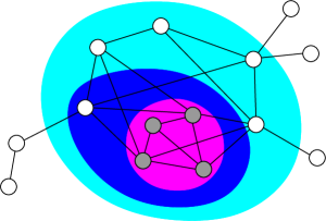
Figure 1: The $(2,2)$-protected core of a small network. The $(2,2)$-protected core (magenta region) is contained in the core (blue), which is then contained in the $2$-core (cyan). Protected and unprotected nodes are colored in gray and white, respectively.

We refer to the above-mentioned evolution process as the $(K,K^{\prime})$-protected core percolation. The $(K,K^{\prime})$-protected core, or simply, the protected core is the subnetwork formed by all the surviving protected nodes and the links among them (see Fig. 1 for an example). We denote the total number of nodes in the protected core as $N_{\mathrm{p\mathchar 45\relax core}}$. We can prove that the protected core is independent of the particular state evolution trajectory of the nodes and hence is well defined (see Supplementary note 1).

In the context of opinion spreading or viral marketing, the $(K,K^{\prime})$-protected core percolation can be described as follows: Consider a population of users to adopt a new product (or idea, opinion, innovation, etc.). Initially there is a $p$ fraction of users in the “protected” (or conservative) state and refuse to adopt the new product. The other $(1-p)$ fraction of users are in the “unprotected” state, i.e., they are early adopters. A conservative user will automatically adopt the new product if he/she has less than $K$ conservative friends. An adopted user with less than $K^{\prime}$ conservative friends will persuade all his or her conservative friends to adopt the new product. Then the protected core, if exists, can be viewed as the subnetwork of the most conservative individuals, who will never adopt the new product.

I.2 Analytical approach.

Consider a large uncorrelated random network containing $N$ nodes, with arbitrary degree distribution $P(k)$ and mean degree $c=\sum_{k\geq 0}kP(k)$ Newman-Strogatz-Watts-2001 ; Molloy-Reed-1995 . We assume that if any node $i$ is still in the protected state, its neighbours do not mutually influence each other and therefore their states are independently distributed. This is a slight extension of the Bethe-Peierls approximation widely used in spin-glass theory and statistical inference Mezard-Montanari-2009 . Note that a closely related approximation in network science is the tree approximation Callaway-etal-2000 ; Cohen-etal-2000 ; Newman-Strogatz-Watts-2001 , which assumes the neighbours of node $i$ become disconnected if $i$ is removed from the network. Under our assumption of state independence we can calculate the normalized size $n_{\mathrm{p\mathchar 45\relax core}}$ ($\equiv N_{\mathrm{p\mathchar 45\relax core}}/N$) of the protected core as

$$n_{\mathrm{p\mathchar 45\relax core}}=p\sum\limits_{s\geq K}\sum\limits_{k\geq s}P(k)C_{k}^{s}(1-\alpha-\beta)^{s}\beta^{k-s}\;,$$ (1)

with $C_{k}^{s}\equiv k!/[s!(k-s)!]$ being the binomial coefficient (Supplementary note 2). The parameter $\alpha$ denotes the probability that, starting from a node $i$ that is still in the protected state, a node $j$ reached by following a randomly chosen link $(i,j)$ is in the unprotected state and having at most $K^{\prime}-1$ protected neighbours (including $i$). The parameter $\beta$ is the probability that such a node $j$ is in the unprotected state but having at least $K^{\prime}$ protected neighbours. We further define $\gamma$ as the probability that such a node $j$ is in the protected state and having exactly $K$ protected neighbours. Note that if initially we randomly choose a finite $p$ fraction of nodes to be protected, then $(1-p)$ fraction of the nodes will be and remain unprotected. Let us define $\eta$ as the probability that, starting from such an initially unprotected node $m$, a node $n$ reached by following a randomly chosen link $(m,n)$ will eventually be in the unprotected state even if the inducing effect of node $m$ is not considered.

Because of the inducing effect, each node $j$ mediates strong correlations among the states of its neighbouring nodes if it is in the unprotected state. After a careful analysis of all the possible microscopic inducing patterns following the theoretical method of Zhou-2005a ; Zhou-2012 , we obtain a set of self-consistent equations for the probabilities $\alpha$, $\beta$, $\gamma$ and $\eta$:

$$\alpha = (1-p)\sum\limits_{s=0}^{K^{\prime}-2}\sum\limits_{k\geq s+1}Q(k)C_{k-1}^{s}(1-\eta)^{s}\eta^{k-1-s}$$

$$+p\ \biggl{\{}\sum\limits_{s=0}^{K-2}\sum\limits_{k\geq s+1}\sum\limits_{r=0}^{\min(s,K^{\prime}-2)}Q(k)C_{k-1}^{s}C_{s}^{r}(\alpha+\beta)^{k-1-s}(1-\alpha-\beta-\gamma)^{r}\gamma^{s-r}$$

$$+\sum\limits_{s\geq K-1}\sum\limits_{k\geq s+2}\sum\limits_{r=0}^{\min(s,K^{\prime}-2)}Q(k)C_{k-1}^{s}C_{s}^{r}\bigl{[}(\alpha+\beta)^{k-1-s}-\beta^{k-1-s}\bigr{]}(1-\alpha-\beta-\gamma)^{r}\gamma^{s-r}\biggr{\}}\;,$$

$$\beta = (1-p)\sum\limits_{s\geq K^{\prime}-1}\sum\limits_{k\geq s+1}Q(k)C_{k-1}^{s}(1-\eta)^{s}\eta^{k-1-s}$$

$$+ p\ \biggl{\{}\sum\limits_{s=K^{\prime}-1}^{K-2}\sum\limits_{k\geq s+1}\sum\limits_{r=K^{\prime}-1}^{s}Q(k)C_{k-1}^{s}C_{s}^{r}(\alpha+\beta)^{k-1-s}(1-\alpha-\beta-\gamma)^{r}\gamma^{s-r}$$

$$+ \sum\limits_{s\geq\max(K,K^{\prime})-1}\sum\limits_{k\geq s+2}\sum\limits_{r=K^{\prime}-1}^{s}Q(k)C_{k-1}^{s}C_{s}^{r}\bigl{[}(\alpha+\beta)^{k-1-s}-\beta^{k-1-s}\bigr{]}(1-\alpha-\beta-\gamma)^{r}\gamma^{s-r}\biggr{\}}\;,$$

$$\gamma = p\sum\limits_{k\geq K}Q(k)C_{k-1}^{K-1}(1-\alpha-\beta)^{K-1}\beta^{k-K}\;,$$ (4)

$$\eta = 1-p+p\ \biggl{\{}\sum\limits_{s=0}^{K-1}\sum\limits_{k\geq s+1}Q(k)C_{k-1}^{s}(1-\alpha-\beta)^{s}(\alpha+\beta)^{k-1-s}$$ (5)

$$\quad\quad\quad\quad\quad\quad+\sum\limits_{s\geq K}\sum\limits_{k\geq s+2}Q(k)C_{k-1}^{s}\bigl{[}(\alpha+\beta)^{k-1-s}-\beta^{k-1-s}\bigr{]}(1-\alpha-\beta)^{s}\biggr{\}}\;,$$

where $Q(k)\equiv kP(k)/c$ is the degree distribution for the node at an end of a randomly chosen link. These equations can be understood as follows. The first term on the r.h.s. of Eq. (LABEL:eq:alphaprob1) is the probability that a node $j$ reached by following a link $(i,j)$ is initially unprotected and having at most $K^{\prime}-2$ protected neighbours (excluding node $i$) without considering its inducing effect. The other two terms in the r.h.s. of Eq. (LABEL:eq:alphaprob1) yield the probability that an initially protected node $j$ at the end of a link $(i,j)$ will either spontaneously transit to or be induced to the unprotected state and, when it is still in the protected state, at most $K^{\prime}-2$ of its protected neighbours (excluding node $i$) have more than $K$ protected neighbours themselves. The terms in Eqs. (LABEL:eq:betaprob1)-(5) can be understood similarly (see Supplementary note 2 for more explanations).

The above self-consistent equations can be solved using a simple iterative scheme (see Supplementary note 3). When $K,K^{\prime}\geq 2$, these equations always have a trivial solution $(\alpha,\beta,\gamma,\eta)=(1,0,0,1)$, yielding no protected core ($n_{\mathrm{p\mathchar 45\relax core}}=0$). This solution is always locally stable, and it is the only solution if the mean degree $c$ of the network is small or the initial fraction $p$ of protected nodes is small (see Supplementary note 4). As $c$ (or $p$) increases, another stable solution of Eqs. (LABEL:eq:alphaprob1)-(5) appears at the critical mean degree $c=c^{*}$ (or the critical fraction $p=p^{*}$), corresponding to the percolation transition. In the limiting cases of $K\in\{0,1\}$, Equations (LABEL:eq:alphaprob1)-(5) also change from having only one stable solution to having two distinctive stable solutions at certain critical value $c=c^{*}$ or $p=p^{*}$ (see Supplementary note 4).

I.3 The minimal inducing effect.

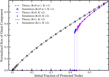
Figure 2: Normalized size of the giant connected component of protected nodes. Symbols are simulation results on a single ER random network of $N=10^{6}$ nodes and mean degree $c=10$, while the lines are theoretical predictions at $N=\infty$. The giant connected component of protected nodes continuously emerges in the $(0,1)$- and $(1,1)$-protected core percolation problems (without inducing effect), but it emerges discontinuously in the $(0,2)$- and $(1,2)$-protected core percolation problems (with minimal inducing effect).

The minimal inducing effect on percolation transitions can be demonstrated by comparing $(0,1)$- and $(1,1)$-protected core percolation transitions with $(0,2)$- and $(1,2)$-protected core percolation transitions as we tune the initial fraction of protected node $p$. Note that the $(K,1)$-protected core percolation with $K\in\{0,1\}$ is essentially the classical site percolation Stauffer-Aharony-1994 ; Cohen-etal-2000 ; Callaway-etal-2000 , because a protected node will remain protected if it has at least one protected neighbour and there is no inducing effect at all. In this case, a giant connected component of protected nodes gradually emerges in the network as $p$ exceeds $p^{*}=1/[\sum_{k\geq 1}(k-1)Q(k)]$ (see Fig. 2). The minimal inducing effect is naturally present in the $(0,2)$- and $(1,2)$-protected core percolation problems, namely if an unprotected node has only one protected neighbour, this neighbour will be induced to the unprotected state. In this case our analytical calculation shows that both the normalized size of the protected core and that of its giant connected component will jump from zero to a finite positive value at certain critical value $p^{*}$ (see Supplementary notes 4 and 5). For Erdös-Rényi (ER) random networks Albert-Barabasi-2002 ; He-Liu-Wang-2009 with mean degree $c=10$, this threshold fraction is $p^{*}\approx 0.44$ (for $K=1$) and $p^{*}\approx 0.42$ (for $K=0$), which are much larger than the threshold value $p^{*}=0.1$ of the classical continuous site percolation transition (see Fig. 2). Note that in case $K=0$, a protected node will never spontaneously become unprotected, hence the discontinuous $(0,2)$-protected core percolation transition is solely due to the inducing effect.

I.4 Inducing effect on $K$-core percolation.

The inducing effect can also be demonstrated by comparing the $K$-core percolation and the $(K,K^{\prime})$-protected core percolation as we tune the mean degree $c$. In the following discussions we set $p=1$ and focus on the representative case of $K^{\prime}=K$ (the results for $p<1$ and $2\leq K^{\prime}\neq K$ are qualitatively the same). And we refer to $(K,K)$-protected core simply as $K$-protected core.

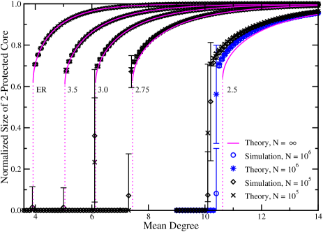
Figure 3: Normalized size of $2$-protected core for ER networks and SF networks. The degree exponents of the SF networks are $\lambda=3.5,3.0,2.75,2.5$ (from left to right). Lines are analytic predictions for infinite system ($N=\infty$), circles and diamonds are exact results obtained through the state evolution process; star and cross symbols are the analytic results using the exact degree sequences of the constructed networks. Each simulation point is obtained by averaging over $80$ independent network instances. Note that for $\lambda<3$, especially when $\lambda\to 2$, significant finite-size effect is observed. This is rooted in the intrinsic degree correlations in the static model when $\lambda<3$ Goh-Kahng-Kim-2001 ; Catanzaro-PastorSatorras-2005 ; Lee-etal-2006 .

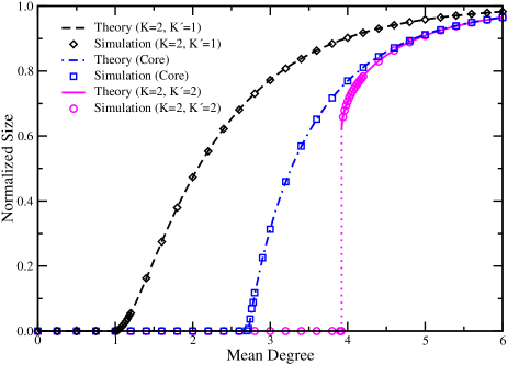
Figure 4: Comparing the percolation transitions. Symbols are simulation results on a single ER random network of $N=10^{6}$ nodes, while the lines are theoretical predictions at $N=\infty$. Both the $2$-core (equivalent to the $(2,1)$-protected core) and the core emerges continuously but the $2$-protected core emerges discontinuously.

We find that for any $K\geq 2$, as $c$ reaches the critical value $c^{*}$, $n_{\mathrm{p\mathchar 45\relax core}}$ jumps from $0$ to a finite value $n_{\mathrm{p\mathchar 45\relax core}}^{*}$ (see Supplementary note 4), indicating a discontinuous percolation transition. We also find that for any $K\geq 2$ and independent of network types, $n_{\mathrm{p\mathchar 45\relax core}}-n_{\mathrm{p\mathchar 45\relax core}}^{*}\propto(c-c^{*})^{1/2}$ in the supercritical regime where $c-c^{*}\to 0^{+}$ (see Supplementary note 6). Such a hybrid phase transition and the associated critical exponent $1/2$ were also observed in $K$-core percolation and core percolation Chalupa-Leath-Reich-1979 ; Pittel-etal-1996 ; Dorogovtsev-etal-2006 ; Liu-etal-2012 .

In the following, we study the discontinuous $2$-protected core percolation in a series of random networks with specific degree distributions. We first consider the ER random network with Poisson degree distribution $P(k)=e^{-c}c^{k}/k!$. We find that the discontinuous $2$-protected core percolation transition occurs at $c=c^{*}\approx 3.92$, with a jump of $n_{\mathrm{p\mathchar 45\relax core}}$ from $0$ to $n_{\mathrm{p\mathchar 45\relax core}}^{*}\approx 0.62$ (see Fig. 3). Note that for ER random networks the classical $2$-core and core percolation transitions occur at $c^{*}=1$ and $c^{*}=e\approx 2.72$, respectively, and they are both continuous Liu-etal-2012 ; Dorogovtsev-etal-2006 . Hence, allowing unprotected nodes to induce other nodes not only delays the occurrence of the percolation transition to a larger value of $c$ but also makes it discontinuous (see Fig. 4).

Scale-free (SF) networks characterized by a power-law degree distribution $P(k)\sim k^{-\lambda}$ with degree exponent $\lambda$ are ubiquitous in real-world complex systems Albert-Barabasi-2002 . Interestingly, we find that for purely scale-free networks with $P(k)=k^{-\lambda}/\zeta(\lambda)$ and $\zeta(\lambda)$ the Riemann $\zeta$ function, the $K$-protected core does not exist for any $\lambda>2$ (see Supplementary note 7). If the smallest degree $k_{\rm min}\geq K$ and a fraction $\rho$ of the links are randomly removed from the purely SF network, then a discontinuous $K$-protected core percolation transition will occur (see Supplementary note 7). For asymptotically SF networks generated by the static model with $P(k)\sim k^{-\lambda}$ for large $k$ only Goh-Kahng-Kim-2001 ; Catanzaro-PastorSatorras-2005 ; Lee-etal-2006 , the $K$-protected core develops when the mean degree $c$ exceeds a threshold value $c^{*}$. For this type of random networks with different values of $c$ and $\lambda$, we compare the theoretical and simulation results and find that they agree well with each other (see Fig. 3).

For random regular (RR) networks, all the nodes have the same degree $k_{0}$, and the $K$-protected core contains the whole network when $k_{0}\geq K$. If a randomly chosen fraction $\rho$ of the links are removed, the degree distribution of the diluted network is given by $P(k)=[k_{0}!/k!(k_{0}-k)!](1-\rho)^{k}\rho^{k_{0}-k}$ with mean degree $c=(1-\rho)k_{0}$. We predict that $n_{\mathrm{p\mathchar 45\relax core}}^{*}\approx 0.77$ (for $k_{0}=4$) and $n_{\mathrm{p\mathchar 45\relax core}}^{*}\approx 0.71$ (for $k_{0}=6$) at the $2$-protected core percolation transition, with $c^{*}\approx 3.08$ and $c^{*}\approx 3.37$, respectively. These predictions are in full agreement with simulation results (see Fig. 5).

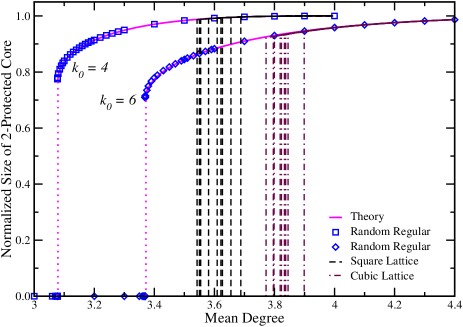
Figure 5: Normalized size of $2$-protected core for RR networks and regular lattices. Solid and dotted lines are analytic predictions for infinite system. Squares and diamonds are simulation results obtained on a diluted RR network instance with node degree $k_{0}=4$ and $k_{0}=6$, respectively, while dashed and long-dashed lines are the simulation results obtained on $20$ independent diluted network instances of the square and cubic lattice. Each simulated network has $N=10^{6}$ nodes.

We also study the $2$-protected core percolation in diluted $D$-dimensional hypercubic lattice and again find a discontinuous transition. Interestingly, in low dimensions the numerically observed transition point $c^{*}$ is remarkably larger than the theoretical prediction (see Figs. 5 and 6). We find that this difference is not a finite-size effect but intrinsic (it remains in the $N\rightarrow\infty$ limit), and the difference decreases quickly as $D$ increases. The transition point $c^{*}$ fluctuates considerably for low dimensions (especially for $D=2,3$) and depends considerably on the system size $N$ (for $D\leq 7$, see Supplementary note 8). Moreover, there is no critical scaling behavior in the supercritical regime (similar absence of critical scaling was also observed in $4$-core percolation on $D=4$ lattices Parisi-Rizzo-2008 ). Surprisingly, the value of $n_{\mathrm{p\mathchar 45\relax core}}$ at and after the percolation transition agrees well with our theoretical prediction (see Fig. 5).

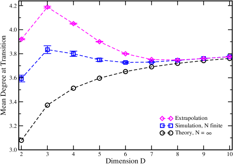
Figure 6: The $2$-protected core percolation transition point $c^{*}$ for the $D$-dimensional hypercubic lattice. Each square is the value of $c^{*}$ obtained by averaging over $1600$ independent diluted network instances with $N\simeq 2\times 10^{6}$ nodes, diamonds are extrapolated simulation results to $N=\infty$, and circles are analytical predictions of $c^{*}$ for an infinite RR network with vertex degree $k_{0}=2D$. The differences between the extrapolated simulation results and the theoretical predictions are due to the ignorance of lattice structures in the theory.

Finally, we apply our theory to a wide range of real-world networks of different sizes and topologies, and find that for most of these networks the normalized sizes of the $2$-protected core can be precisely predicted using the degree distribution as the only input (see Supplementary Tables 1 and 2 and Supplementary note 9).

II Discussion

Inducing effect plays an important role in many complex networked systems. Yet, little was known about how it will affect classical percolation transitions in complex networks. Here we develop analytical tools to address this problem for arbitrary network topologies. Our key finding, that the local inducing effect causes discontinuous site percolation and $K$-core percolation (for any $K\geq 1$), suggests a simple local mechanism to better understand and ultimately predict many abrupt breakdown phenomena observed in various systems, e.g., the global failure of a national-wide power grid, the sudden collapse of a governmental system or a network of financial institutions.

The results presented here also raise a number of questions, answers to which could further deepen our understanding of complex networked systems. First of all, we can improve the local inducing mechanism to be more realistic, e.g., by considering that the parameters $K$ and $K^{\prime}$ might be different for different nodes, an unprotected node may only be able to induce some particular neighbours (e.g., in a directed network), or an unprotected node may recover to the protected state with certain rate, etc.. Secondly, for low-dimensional lattice systems, the lattice structures and the associated short loops cause strong local and long-range correlations among the states of the nodes, which should be properly considered in a future refined theory, e.g., by changing the form of $Q(k)$ to include local degree-degree correlations and by exactly computing the effects of short loops up to certain length. Finally, an interesting optimization problem consists of identifying a minimal set of nodes such that perturbing these nodes to the unprotected state will cause the protected core of the whole network to breakdown. In the context of opinion dynamics or viral marketing, this amounts to identifying a minimal set of users for targeted advertisement so that we can dissolve the protected core and eventually all the users will adopt the new opinion or product. We hope our work will stimulate further research efforts on these and other related interesting and challenging questions.

Acknowledgement

J.-H. Zhao and H.-J. Zhou thank Prof. Zhong-Can Ou-Yang for support and Hong-Bo Jin for technical assistance on computer simulation. J.-H. Zhao and H.-J. Zhou were supported by the National Basic Research Program of China (No. 2013CB932804), the Knowledge Innovation Program of Chinese Academy of Sciences (No. KJCX2-EW-J02), and the National Science Foundation of China (grant Nos. 11121403, 11225526). Y.-Y. Liu was supported by the Network Science Collaborative Technology Alliance under Agreement Number W911NF-09-2-0053, the Defense Advanced Research Projects Agency under Agreement Number 11645021, the Defense Threat Reduction Agency-WMD award numbers HDTRA1-08-1-0027 and HDTRA1-10-1-0100, and the generous support of Lockheed Martin.

Author Contributions H.-J. Zhou conceived research; H.-J. Zhou, J.-H. Zhao and Y.-Y. Liu performed research; H.-J. Zhou and Y.-Y. Liu wrote the paper.

Competing Interests The authors declare that they have no competing financial interests.

Correspondence Correspondence should be addressed to H.-J. Zhou (email: zhouhj@itp.ac.cn).

Table 1: List of $37$ real-world networks analyzed in this work. For each network, we show its type, name, reference and brief description.

	Name	Description
Regulatory	TRN-Yeast-1 [51]	Transcriptional regulatory network of S. cerevisiae
	TRN-Yeast-2 [52]	Same as above (compiled by different group).
	TRN-EC-1 [53]	Transcriptional regulatory network of E. coli
	TRN-EC-2 [52]	Same as above (compiled by different group).
	Ownership-USCorp [54]	Ownership network of US corporations.
Trust	College student [55,56]	Social networks of positive sentiment (college students).
	Prison inmate [55,56]	Same as above (prison inmates).
	Slashdot [57]	Social network (friend/foe) of Slashdot users.
	WikiVote [57]	Who-vote-whom network of Wikipedia users.
	Epinions [58]	Who-trust-whom network of Epinions.com users.
Food Web	Ythan [59]	Food Web in Ythan Estuary.
	Little Rock [60]	Food Web in Little Rock lake.
	Grassland [59]	Food Web in Grassland.
	Seagrass [61]	Food Web in St. Marks Seagrass.
Power Grid	TexasPowerGrid [62]	Power grid in Texas.
Metabolic	E. coli [63]	Metabolic network of E. coli.
	S. cerevisiae [63]	Metabolic network of S. cerevisiae.
	C. elegans [63]	Metabolic network of C. elegans.
Electronic	s838 [52]	Electronic sequential logic circuit.
Circuits	s420 [52]	Same as above.
	s208 [52]	Same as above.
Neuronal	C. elegans [64]	Neural network of C. elegans.
Citation	ArXiv-HepTh [65]	Citation networks in HEP-TH category of Arxiv.
	ArXiv-HepPh [65]	Citation networks in HEP-PH category of Arxiv.
WWW	nd.edu [66]	WWW from nd.edu domain.
	stanford.edu [57]	WWW from stanford.edu domain.
	Political blogs [67]	Hyperlinks between weblogs on US politics.
Internet	p2p-1 [68]	Gnutella peer-to-peer file sharing network.
	p2p-2 [68]	Same as above (at different time).
	p2p-3 [68]	Same as above (at different time).
Social	UCIonline [69]	Online message network of students at UC, Irvine.
Communication	Email-epoch [70]	Email network in a university.
	Cellphone [71]	Call network of cell phone users.
Intra-	Freemans-2 [72]	Social network of network researchers.
organizational	Freemans-1 [72]	Same as above (at different time).
	Manufacturing [73]	Social network from a manufacturing company.
	Consulting [73]	Social network from a consulting company.

Table 2: $2$-protected core size of $37$ real-world networks. For each network, we show its type, name; number of nodes ($N$) and links ($M$); number of protected nodes in the $2$-protected core ($N_{\mathrm{p\mathchar 45\relax core}}^{\rm real}$); normalized size of $2$-protected core ($n_{\mathrm{p\mathchar 45\relax core}}^{\rm real}$), and theoretical prediction of normalized size of $2$-protected core ($n_{\mathrm{p\mathchar 45\relax core}}^{\rm theory}$). In the last two columns, if empirical value and theoretical prediction are significantly different, these items are highlighted by bold type.

	Name	$N$	$M$	$N_{\mathrm{p\mathchar 45\relax core}}^{\rm real}$	$n_{\mathrm{p\mathchar 45\relax core}}^{{\rm real}}$	$n_{\mathrm{p\mathchar 45\relax core}}^{{\rm theory}}$
Regulatory	TRN-Yeast-1	4,441	12,864	0	0	0
	TRN-Yeast-2	688	1,078	0	0	0
	TRN-EC-1	1,550	3,234	24	0.0155	0
	TRN-EC-2	418	519	0	0	0
	Ownership-USCorp	7,253	6,711	8	0.0011	0
Trust	College student	32	80	32	1	1
	Prison inmate	67	142	58	0.8657	0.7970
	Slashdot	82,168	504,230	229	0.0028	0
	WikiVote	7,115	100,762	0	0	0
	Epinions	75,888	405,740	261	0.0034	0
Food Web	Ythan	135	596	0	0	0
	Little Rock	183	2,434	181	0.9891	0.9889
	Grassland	88	137	0	0	0
	Seagrass	49	223	49	1	1
Power Grid	TexasPowerGrid	4,889	5,855	4	0.0008	0
Metabolic	E. coli	2,275	5,627	148	0.0651	0
	S. cerevisiae	1,511	3,807	311	0.2058	0
	C. elegans	1,173	2,842	806	0.6871	0
Electronic	s838	512	819	0	0	0
Circuits	s420	252	399	0	0	0
	s208	122	189	0	0	0
Neuronal	C. elegans	297	2,148	272	0.9158	0.8962
Citation	ArXiv-HepTh	27,770	352,285	23379	0.8419	0.8477
	ArXiv-HepPh	34,546	420,877	30704	0.8888	0.9075
WWW	nd.edu	325,729	1,090,108	85,469	0.2624	0
	stanford.edu	281,903	1,992,636	210,612	0.7471	0
	Political blogs	1,224	16,715	0	0	0.5763
Internet	p2p-1	10,876	39,994	0	0	0
	p2p-2	8,846	31,839	0	0	0
	p2p-3	8,717	31,525	0	0	0
Social	UCIonline	1,899	13,838	0	0	0
Communication	Email-epoch	3,188	31,857	0	0	0
	Cellphone	36,595	56,853	804	0.0220	0
Intra-	Freemans-2	34	474	34	1	1
organizational	Freemans-1	34	415	34	1	1
	Manufacturing	77	1,341	77	1	1
	Consulting	46	550	46	1	1

Supplementary Note 1

The $(K,K^{\prime})$-protected core of a network only depends on the initial states of the nodes. Here we prove that the same final $(K,K^{\prime})$-protected core will be reached independent of the particular state evolution trajectory of the nodes.

Proof: Let us suppose the contrary is true, namely there exist two different patterns (say $P_{1}$ and $P_{2}$) of final states for a given network. Denote by $S_{pp}$ the set of nodes that are in the protected state in both patterns $P_{1}$ and $P_{2}$, by $S_{uu}$ the set of nodes that are in the unprotected state in both patterns, and by $S_{pu}$ the set of nodes that are in the protected state in one pattern but are in the unprotected state in the other pattern. These three sets are mutually exclusive and their union contains all the nodes of the network. Because $P_{1}$ and $P_{2}$ are two different state patterns, the set $S_{pu}$ must be non-empty.

Consider a node $i\in S_{pu}$. By definition, node $i$ is protected in one pattern (say $P_{1}$) and unprotected in the other pattern ($P_{2}$). Since $i$ has the final protected state in pattern $P_{1}$, its final unprotected state in $P_{2}$ must not be induced by any of the unprotected nodes of set $S_{uu}$. Therefore, the protected-to-unprotected flipping of node $i$ in pattern $P_{2}$ must be preceded by at least one protected-to-unprotected flipping in pattern $P_{2}$ of another node $j\in S_{pu}$. But not all nodes of the set $S_{pu}$ can have this property. Therefore the set $S_{pu}$ must be empty and the two state patterns $P_{1}$ and $P_{2}$ must be identical. This proves the uniqueness of the $(K,K^{\prime})$-protected core.

Supplementary Note 2

We give more explanations on the mean field equations (1)-(5) of the main text. First consider a randomly chosen node $i$ that is initially in the protected state. The probability that this node has $k$ neighbours is just $P(k)$. We assume that, given the central node $i$ is still in the protected state, the states of its neighbouring nodes are completely independent of each other. Under this assumption we then obtain that, given node $i$ being in the protected state, the probability that $s$ of its neighbours are also in the protected state and $r$ of its neighbours are in the unprotected state with less than $K^{\prime}$ protected neighbours while the remaining $k-s-r$ neighbours are in the unprotected state with at least $K^{\prime}$ protected neighbours is expressed as

$$\frac{k!}{s!r!(k-s-r)!}(1-\alpha-\beta)^{s}\alpha^{r}\beta^{k-s-r}\;.$$

For node $i$ to remain in the protected state, the number $r$ must be zero and the number $s$ must be equal or greater than $K$. In other words, the probability for an initially protected node $i$ to keep its initial state is

$$\sum_{s=K}^{k}C_{k}^{s}(1-\alpha-\beta)^{s}\beta^{k-s}\;,$$

with $C_{k}^{s}\equiv k!/[s!(k-s)!]$ being the binomial coefficient. After considering all the possible values of the node degree $k$, we then obtain the expression (1) concerning the normalized size $n_{\mathrm{p\mathchar 45\relax core}}$ of the protected core, which is also the probability that a randomly chosen node $i$ is in the protected state.

We continue to discuss the expressions for $\alpha$, $\beta$ and $\gamma$ following the theoretical approach of Refs. [37, 38]. Consider a node $j$ that is neighbouring to a protected node $i$. In an uncorrelated network, the probability of node $j$ to have $k$ neighbours is expressed as

$$Q(k)=\frac{kP(k)}{c}\;,$$ (6)

with $c\equiv\sum_{k}kP(k)$ being the mean node degree of the network. For node $j$ to be in the protected state with exactly $K$ protected neighbours, it must have $K-1$ other protected neighbours besides node $i$, and it must not be connected to any unprotected node with less than $K^{\prime}$ protected neighbours. These conditions lead to the expression (4) for the probability $\gamma$.

If node $j$ is initially in the unprotected state but is not able to induce other protected nodes, it must have $s\geq K^{\prime}-1$ other protected neighbours besides node $i$. This leads to the first term on the r.h.s. of Eq. (3). If node $j$ is initially in the protected state but having less than $K$ protected neighbours, it will spontaneously become unprotected. If node $j$ is initially in the protected state but having at least $K$ protected neighbours, it will be induced to the unprotected state if $j$ is connected to at least one unprotected node (say node $l$) which has less than $K^{\prime}$ protected neighbours when node $j$ is still in the protected state. Some of the protected neighbours (excluding node $i$) of node $j$ may have exactly $K$ protected neighbours when $j$ is still in the protected state. Such nodes are referred to as critical protected nodes. All these critical protected nodes will spontaneously become unprotected after node $j$ becomes unprotected. If the remaining number of protected neighbours of node $j$ is still at least $K^{\prime}$ after all these critical protected nodes become unprotected, node $j$ will not be able to induce these remaining protected nodes. The second term on the r.h.s. of Eq. (3) is just the total probability for this situation to occur.

If node $j$ is initially in the unprotected state and having less than $K^{\prime}$ protected neighbours, it will be able to induce node $i$ and all its other protected neighbours to the unprotected state. This situation corresponds to the first term on the r.h.s. of Eq. (2). If node $j$ is initially in the protected state but having less than $K$ protected neighbours, it will spontaneously become unprotected. If node $j$ is initially in the protected state and having $K$ or more protected neighbours, it will be induced to the unprotected state if at least one of its unprotected neighbours has less than $K^{\prime}$ protected neighbours. Some of the protected neighbours (excluding node $i$) of node $j$ may have exactly $K$ protected neighbours when $j$ is still in the protected state. All these critical protected nodes will spontaneously become unprotected after node $j$ has changed to the unprotected state. The number of protected neighbours of node $j$ may become less than $K^{\prime}$ after all these critical protected nodes have transited to the unprotected state. If this is the case, node $j$ will then be able to induce its remaining protected neighbours to the unprotected state. The second term on the r.h.s. of Eq. (2) is just the total probability for this situation to occur.

To understand the expression (5) for the probability $\eta$, let us consider a neighbouring node $n$ of an initially unprotected node $m$. If $n$ is initially unprotected (with probability $1-p$), it will remain in the unprotected state. If $n$ is initially protected but having less than $K$ protected neighbours, it will spontaneously become unprotected. If node $n$ is initially protected and having $K$ or more protected neighbours, it will be induced to the unprotected state if at least one of its unprotected neighbours (excluding node $m$) has less than $K^{\prime}$ protected neighbours. The two terms inside the curly brackets of Eq. (5) are the probabilities for the initial protected node $n$ to spontaneously become unprotected and to be induced to the unprotected state, respectively.

Supplementary Note 3

The mean field equations (1)-(5) work both for finite networks and infinite networks ($N=\infty$). The only input to these equations is the degree distribution $P(k)$. The other degree distribution $Q(k)$ is determined from $P(k)$ through Eq. (6). Here we introduce a simple numerical scheme for determining the values of $\alpha$, $\beta$, $\gamma$ and $\eta$.

From Eqs. (2) and (3) we obtain that

$$\beta=g(\beta)\equiv 1-\alpha-p\sum\limits_{k\geq K}Q(k)\sum\limits_{s\geq K-1}^{k-1}C_{k-1}^{s}\beta^{k-1-s}(1-\alpha-\beta)^{s}\;.$$ (7)

The value of $\beta$ can be obtained by solving $\beta=g(\beta)$ at each fixed value of $\alpha$. When $K\geq 2$, this equation always has a solution $\beta=1-\alpha$. After the value of $\beta$ is determined from $\alpha$, then the value of $\gamma$ and the value of $\eta$ can be obtained through Eq. (4) and Eq. (5), respectively, using the values of $\alpha$ and $\beta$ as inputs. Notice that for $K\geq 2$, if $\beta=1-\alpha$ then $\gamma=0$ and $\eta=1$.

After the values of $\beta$, $\gamma$ and $\eta$ are obtained at a given value of $\alpha$, then we can obtain a new value of $\alpha$ through Eq. (2). In this way a mapping $\alpha\leftarrow f(\alpha)$ from $\alpha$ to $\alpha$ is constructed for $0\leq\alpha\leq 1$. The mapping function $f(\alpha)$ is just the r.h.s. of Eq. (2), namely

$$f(\alpha) = (1-p)\sum\limits_{s=0}^{K^{\prime}-2}\sum\limits_{k\geq s+1}Q(k)C_{k-1}^{s}(1-\eta)^{s}\eta^{k-1-s}$$

$$+p\ \biggl{\{}\sum\limits_{s=0}^{K-2}\sum\limits_{k\geq s+1}\sum\limits_{r=0}^{\min(s,K^{\prime}-2)}Q(k)C_{k-1}^{s}C_{s}^{r}(\alpha+\beta)^{k-1-s}(1-\alpha-\beta-\gamma)^{r}\gamma^{s-r}$$

$$+\sum\limits_{s\geq K-1}\sum\limits_{k\geq s+2}\sum\limits_{r=0}^{\min(s,K^{\prime}-2)}Q(k)C_{k-1}^{s}C_{s}^{r}\bigl{[}(\alpha+\beta)^{k-1-s}-\beta^{k-1-s}\bigr{]}(1-\alpha-\beta-\gamma)^{r}\gamma^{s-r}\biggr{\}}\;,$$

in which $\beta$, $\gamma$ and $\eta$ are all regarded as functions of $\alpha$. By solving the equation $\alpha=f(\alpha)$ we obtain the value of $\alpha$, which then fixes the values of $\beta$, $\gamma$ and $\eta$. For $K\geq 2$ and $K^{\prime}\geq 2$, it can be easily checked that $\alpha=1$ is always a solution of the equation $\alpha=f(\alpha)$.

Denote a generic solution of the equation $\alpha=f(\alpha)$ as $\alpha_{0}$. If starting from a value of $\alpha$ slightly different from $\alpha_{0}$, the iteration $\alpha\leftarrow f(\alpha)$ can drive $\alpha$ back to $\alpha_{0}$, then we regard $\alpha_{0}$ as a locally stable solution of $\alpha=f(\alpha)$. Otherwise $\alpha_{0}$ is regarded as an unstable solution of this equation.

Supplementary Note 4

We explain that the mean field equations (1)-(5) predict the $(K,K^{\prime})$-protected core percolation transition to be discontinuous if $K^{\prime}\geq 2$, independent of the value of $K$. We begin with the simpler cases of $K=2$ and $K\geq 3$, and then discuss the more difficult cases of $K=1$ and $K=0$.

(a) $K=2$

Figure 7: Function $g(\beta)$ at $K=K^{\prime}=2$ for the infinite ER random network with mean degree $c=4$. The initial fraction of protected nodes is $p=1$, and the probability $\alpha$ is $\alpha=0.2$ or $\alpha=0.4$. Both $g(\beta)$ and $\beta$ are normalized by $(1-\alpha)$ so that all the curves meet at the point $\beta/(1-\alpha)=1$. The solutions of the equation $\beta=g(\beta)$ can be read off from the crossing points of the $g(\beta)$ curve with the dashed line representing $\beta=\beta$. At $\alpha=0.4$ there is only one solution, while at $\alpha=0.2$ there are two solutions.

A protected node will spontaneously become unprotected if it has less than two protected neighbours. The function $g(\beta)$ is expressed as

$$g(\beta)=1-\alpha-p\sum\limits_{k\geq 1}Q(k)\bigl{[}(1-\alpha)^{k-1}-\beta^{k-1}\bigr{]}\;.$$ (9)

The first derivative of $g(\beta)$ with respective to $\beta$ is simply

$$\frac{\partial g(\beta)}{\partial\beta}=p\sum\limits_{k\geq 2}(k-1)Q(k)\beta^{k-2}\;,$$ (10)

which increases with $\beta$. Therefore $g(\beta)$ as a function of $\beta$ is convex in the interval $0\leq\beta\leq 1-\alpha$, see Fig. 7 for some examples obtained from the Erdös-Rényi (ER) random network of mean degree $c=4$. If $p\sum_{k\geq 2}(k-1)Q(k)>1$, then there exists a value of $\alpha_{t}$ such that

$$\left.\frac{\partial g(\beta)}{\partial\beta}\right|_{\beta=1-\alpha}\equiv p\sum_{k\geq 2}(k-1)Q(k)(1-\alpha)^{k-2}<1$$

for $\alpha>\alpha_{t}$. Notice that $\alpha_{t}$ is strictly less than $1$. Then for $\alpha\in[\alpha_{t},1]$, the equation $\beta=g(\beta)$ has only a unique solution $\beta=1-\alpha$. If $p\sum_{k\geq 2}(k-1)Q(k)\leq 1$, then $\left.\frac{\partial g(\beta)}{\partial\beta}\right|_{\beta=1-\alpha}\leq 1$ at any value of $\alpha\in[0,1]$. This means the solution of $\beta=g(\beta)$ is always $\beta=1-\alpha$ for any $\alpha_{t}\leq\alpha\leq 1$ with $\alpha_{t}=0$.

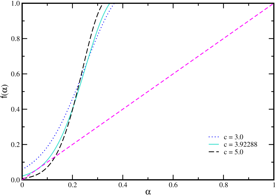
Figure 8: Function $f(\alpha)$ at $K=K^{\prime}=2$ for the infinite ER random network. The initial fraction of protected nodes is set to $p=1$, and the mean degree is $c=3.0$ (dotted line), $c=3.92288$ (solid line), or $c=5.0$ (long-dashed line). The function $f(\alpha)=1$ for $\alpha$ sufficiently close to $1$. When $c<3.92288$ the equation $\alpha=f(\alpha)$ has only the solution $\alpha=1$. When $c>3.92288$, there are three solutions of $\alpha=f(\alpha)$ as can be read off from the crossing points of $f(\alpha)$ with the dashed line representing $\alpha=\alpha$: the solutions $\alpha=1$ and the one with $\alpha\approx 0$ are stable, while the middle one is unstable.

From these discussions, we know that there exists a value $\alpha_{t}$ strictly less than $1$ such that $f(\alpha)=1$ for $\alpha_{t}\leq\alpha\leq 1$. Some example curves of $f(\alpha)$ are shown in Fig. 8 for infinite ER random networks. If $\alpha_{t}=0$, then $\alpha=1$ is the only solution of $\alpha=f(\alpha)$. If $0<\alpha_{t}<1$, then $f(\alpha_{t})=1>\alpha_{t}$ (notice that $\beta=1-\alpha_{t}$ at $\alpha=\alpha_{t}$). Consequently if $\alpha=f(\alpha)$ has another solution different from $\alpha=1$, this solution $\alpha$ must be strictly less than $\alpha_{t}$, and $\alpha+\beta$ at this solution must be strictly less than $1$.

According to Eq. (1), the normalized size of the protected core $n_{\mathrm{p\mathchar 45\relax core}}=0$ if $\alpha+\beta=1$. On the other hand, if $\alpha+\beta<1$ then $n_{\mathrm{p\mathchar 45\relax core}}$ will be strictly positive. We therefore conclude that, if the $(2,K^{\prime})$-protected core percolation transition occurs in a network, the normalized size of the $(2,K^{\prime})$-protected core will have a finite jump at the transition point.

(b) $K\geq 3$

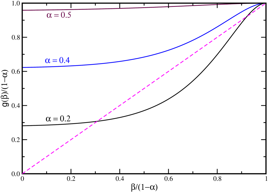
Figure 9: Function $g(\beta)$ at $K=K^{\prime}=3$ for the infinite ER random network with mean degree $c=7.5$. The initial fraction of protected nodes is $p=1$, and the probability $\alpha$ is $\alpha=0.2$, $0.4$ or $0.5$. Both $g(\beta)$ and $\beta$ are normalized by $(1-\alpha)$ so that all the curves meet at the point $\beta/(1-\alpha)=1$. The solutions of the equation $\beta=g(\beta)$ can be read off from the crossing points of the $g(\beta)$ curve with the dashed line representing $\beta=\beta$.

The function $g(\beta)$ has the following expression

$$g(\beta)=1-\alpha-p\sum\limits_{k\geq K}Q(k)\sum\limits_{s=K-1}^{k-1}C_{k-1}^{s}(1-\alpha-\beta)^{s}\beta^{k-1-s}\;.$$ (11)

Some representative curves of $g(\beta)$ are shown in Fig. 9 for the infinite ER random network of mean degree $c=7.5$. The first derivative of $g(\beta)$ with respective to $\beta$ is

$$\frac{\partial g(\beta)}{\partial\beta}=p\sum\limits_{k\geq K}(k-1)Q(k)C_{k-2}^{K-2}\beta^{k-K}(1-\alpha-\beta)^{K-2}\;.$$ (12)

At $\beta=1-\alpha$ this derivative is equal to $0$. There exists a threshold value $\alpha_{t}<1$ such that if $\alpha\geq\alpha_{t}$ then $\frac{\partial g(\beta)}{\partial\beta}<1$ for $0\leq\beta\leq 1-\alpha$. Therefore for $\alpha\in[\alpha_{t},1]$ the equation $\beta=g(\beta)$ has only the unique solution $\beta=1-\alpha$.

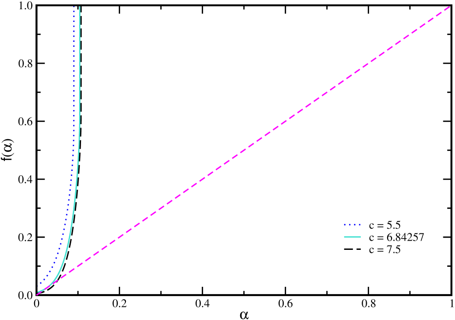
Figure 10: Function $f(\alpha)$ at $K=K^{\prime}=3$ for the infinite ER random network. The initial fraction of protected nodes is set to $p=1$, and the mean degree is $c=5.5$ (dotted line), $c=6.68257$ (solid line), or $c=7.5$ (long-dashed line). The function $f(\alpha)=1$ for $\alpha$ sufficiently close to $1$. When $c<6.68257$ the equation $\alpha=f(\alpha)$ has only the solution $\alpha=1$. When $c>6.68257$, there are three solutions of $\alpha=f(\alpha)$ as can be read off from the crossing points of $f(\alpha)$ with the dashed line representing $\alpha=\alpha$.

Due to the fact that $\left.\frac{\partial g(\beta)}{\partial\beta}\right|_{\beta=1-\alpha}=0$, if for some values of $\alpha<\alpha_{t}$ the equation $\beta=g(\beta)$ has another solution with $\beta\neq 1-\alpha$, then at this solution the sum $\alpha+\beta$ must be strictly less than $1$ (the behaviour of $g(\beta)$ at $\beta/(1-\alpha)\approx 1$ is demonstrated in Fig. 9). Since $\beta=1-\alpha$ for $\alpha>\alpha_{t}$, then the function $f(\alpha)=1$ for $\alpha\in[\alpha_{t},1]$ (see Fig. 10 for some representative curves of $f(\alpha)$ for the infinite ER random network). If another stable solution of $\alpha=f(\alpha)$ exists, the value of $\alpha$ at this solution must be strictly less than $\alpha_{t}$, and the value of $\alpha+\beta$ must be strictly less than $1$.

According to Eq. (1), the normalized size of the protected core $n_{\mathrm{p\mathchar 45\relax core}}=0$ if $\alpha+\beta=1$. On the other hand, if $\alpha+\beta<1$ then $n_{\mathrm{p\mathchar 45\relax core}}$ will be strictly positive. We therefore conclude that, for $K\geq 3$, if the $(K,K^{\prime})$-protected core percolation transition occurs in a network, the normalized size of the $(K,K^{\prime})$-protected core will have a finite jump at the transition point.

(c) $K=1$

In this case, a protected node will spontaneously become unprotected if it has no protected neighbour. From the mean field equations (2)-(5) we obtain that

$$\beta = 1-\alpha-p\sum\limits_{k\geq 1}Q(k)(1-\alpha)^{k-1}\;,$$ (13)

$$\gamma = p\sum\limits_{k\geq 1}Q(k)\beta^{k-1}\;,$$ (14)

$$\eta = \alpha+\beta+\gamma\;.$$ (15)

The function $f(\alpha)$, namely the expression (LABEL:eq:falpha) with $\beta,\gamma,\eta$ determined from $\alpha$ through the above three equations, is a smooth function of $\alpha$ (some example curves of $f(\alpha)$ are shown in Fig. 11 for the infinite ER random network with mean degree $c=4$). We can easily verify that $f(0)>0$.

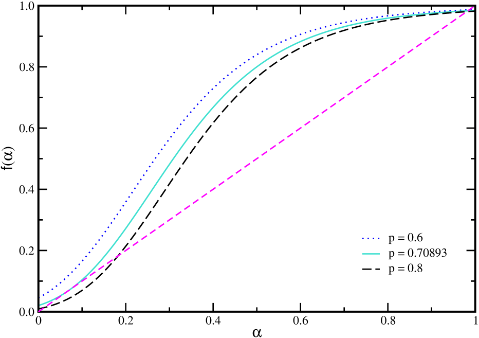
Figure 11: Function $f(\alpha)$ at $K=1$ and $K^{\prime}=2$ for the infinite ER random network with mean degree $c=4$. The initial fraction of protected nodes is $p=0.6$ (dotted line), $p=0.70893$ (solid line), or $p=0.8$ (long-dashed line). When $p<0.70893$ the equation $\alpha=f(\alpha)$ has only one solution, located at $\alpha\approx 1$. When $p>0.70893$, there are three solutions of $\alpha=f(\alpha)$ as can be read off from the crossing points of $f(\alpha)$ with the dashed line representing $\alpha=\alpha$.

Denote $\alpha_{\rm max}$ as the largest root of the equation

$$\alpha=1-p\sum\limits_{k\geq 1}Q(k)(1-\alpha)^{k-1}\;$$ (16)

in the interval of $0\leq\alpha\leq 1$. If $pQ(1)=0$, then $\alpha_{\rm max}=1$; if $0<pQ(1)<1$ then $0<\alpha_{\rm max}<1$; if $pQ(1)=1$ then $\alpha_{\rm max}=0$. The last case is not interesting: $pQ(1)=1$ means that $Q(1)=1$ (all the nodes have only one neighbour) and $p=1$ (all the nodes are initially in the protected state), then the states of the nodes will not change with time. We assume that $pQ(1)<1$ in the following discussions (i.e., $\alpha_{\rm max}>0$).

When $0\leq\alpha<\alpha_{\rm max}$ the value of $\beta$ as obtained by Eq. (13) is positive. The value of $\beta$ reduces to zero at $\alpha=\alpha_{\rm max}$. We can verify that $f(\alpha_{\rm max})<\alpha_{\rm max}$. To prove this statement, let us first write $f(\alpha)$ as

$$f(\alpha) = 1-p\sum\limits_{k\geq 1}Q(k)(1-\alpha)^{k-1}$$ (17)

$$-p\sum\limits_{k\geq K^{\prime}}Q(k)\sum\limits_{s=K^{\prime}-1}^{k-1}C_{k-1}^{s}\bigl{[}(\alpha+\beta)^{k-1-s}-\beta^{k-1-s}\bigr{]}\sum\limits_{r=K^{\prime}-1}^{s}C_{s}^{r}(1-\alpha-\beta-\gamma)^{r}\gamma^{s-r}$$

$$-(1-p)\sum\limits_{k\geq K^{\prime}}Q(k)\sum\limits_{s=K^{\prime}-1}^{k-1}C_{k-1}^{s}(1-\eta)^{s}\eta^{k-1-s}\;.$$

Since the third and fourth term on the r.h.s. of the above expression are both negative, we obtain that $f(\alpha)<1-p\sum_{k\geq 1}Q(k)(1-\alpha)^{k-1}$. It then follows that $f(\alpha_{\rm max})<\alpha_{\rm max}$.

Because $f(\alpha)>\alpha$ at $\alpha=0$ and $f(\alpha)<\alpha$ at $\alpha=\alpha_{\rm max}$, the curve $f(\alpha)$ will intersect with the rectilinear line $\alpha=\alpha$ either once or three times in the interval $\alpha\in(0,\alpha_{\rm max})$. This fact is demonstrated clearly in Fig. 11. In other words, the equation $\alpha=f(\alpha)$ either has only a single solution in the interval $\alpha\in(0,\alpha_{\rm max})$ or has three solutions in this interval. In the latter case, since the function $f(\alpha)$ is a smooth function, there must be a finite gap between the two stable solutions, with one stable solution located at $\alpha\approx 0$ (corresponding to a value of $n_{\mathrm{p\mathchar 45\relax core}}$ well above zero) and the other stable solution at $\alpha\approx\alpha_{\rm max}$ (corresponding to a value of $n_{\mathrm{p\mathchar 45\relax core}}\approx 0$).

(d) $K=0$

In this case, an initially protected node will never spontaneously become unprotected. It can only be induced to the unprotected by a neighbouring unprotected node. This case is actually very similar to the case of $K=1$. For example the mean field equation for $\beta$ is the same as Eq. (13). The only difference is that $\gamma=0$ in this limiting case.

We can follow the same theoretical arguments developed for the case of $K=1$ to prove that, if a $(0,K^{\prime})$-protected core percolation transition occurs in a network, the normalized size of the protected core at the transition point must has a finite jump from nearly zero to a positive value well above zero.

Supplementary Note 5

Here we list the explicit mean field equations for computing the the sizes of $(0,1)$-protected core, $(1,1)$-protected core, $(0,2)$-protected core, and $(1,2)$-protected core, respectively.

(a) $K=1,K^{\prime}=1$ (minimal spontaneous transition, no inducing effect)

In this case, an unprotected node is not able to induce its protected neighbours. An initially protected node will spontaneously become unprotected only if all its neighbours are initially unprotected.

The fraction of protected nodes in the final state is

$$n_{\mathrm{p\mathchar 45\relax core}}(1,1)=p\Bigl{[}1-\sum\limits_{k\geq 0}P(k)(1-p)^{k}\Bigr{]}\;.$$ (18)

The normalized size $g_{\mathrm{p\mathchar 45\relax core}}(1,1)$ of the giant component of protected nodes is expressed as

$$g_{\mathrm{p\mathchar 45\relax core}}(1,1)=p\Bigl{[}1-\sum\limits_{k\geq 0}P(k)\mu^{k}\Bigr{]}\;,$$ (19)

where $\mu$ is the probability that, starting from a protected node $i$, the node $j$ reached by following a randomly chosen link $(i,j)$ is not belonging to the giant connected component of protected nodes if the link $(i,j)$ is absent. The expression for $\mu$ is

$$\mu=1-p+p\sum\limits_{k\geq 1}Q(k)\mu^{k-1}\;.$$ (20)

If $p\sum_{k\geq 2}(k-1)Q(k)\leq 1$, Eq. (20) has only a single solution $\mu=1$ (no giant component of protected nodes). Equation (20) has a stable solution with $\mu<1$ when $p\sum_{k\geq 2}(k-1)Q(k)>1$, corresponding to the existence of a giant connected component of protected nodes.

(b) $K=0,K^{\prime}=1$ (no spontaneous transition and no inducing effect)

Since an initially protected node will never spontaneously become unprotected (because $K=0$) nor be induced to the unprotected state (because $K^{\prime}=1$), there is no any state evolution in the system. The fraction of protected nodes in the final steady state is just $p$. The normalized size $g_{\mathrm{p\mathchar 45\relax core}}(0,1)$ of the giant connected component of protected nodes has the same expression as Eq. (19), with the probability $\mu$ determined by Eq. (20).

(c) $K=1,K^{\prime}=2$ (minimal spontaneous transition and minimal inducing effect)

In this case, if an unprotected node has only a single protected neighbour, it can induce this node to the unprotected state. An initially protected node will spontaneously become unprotected only if all of its neighbours are unprotected. The fraction of protected nodes at the steady state is

$$n_{\mathrm{p\mathchar 45\relax core}}(1,2)=p\sum\limits_{k}P(k)\bigl{[}(1-\alpha)^{k}-\beta^{k}\bigr{]}\;.$$ (21)

The expressions for $\alpha$, $\beta$, $\gamma$ and $\eta$ are, respectively

$$\alpha = (1-p)\sum\limits_{k\geq 1}Q(k)\eta^{k-1}+p\sum\limits_{k\geq 1}Q(k)\bigl{[}(\alpha+\beta+\gamma)^{k-1}-(\beta+\gamma)^{k-1}\bigr{]}\;,$$ (22)

$$\beta = 1-(1-p)\sum\limits_{k\geq 1}Q(k)\eta^{k-1}$$ (23)

$$\quad\quad\quad+p\sum\limits_{k\geq 1}Q(k)\bigl{[}(\beta+\gamma)^{k-1}-(\alpha+\beta+\gamma)^{k-1}-(1-\alpha)^{k-1}\bigr{]}\;,$$

$$\gamma = p\sum\limits_{k\geq 1}Q(k)\beta^{k-1}\;,$$ (24)

$$\eta = 1-p\sum\limits_{k\geq 1}Q(k)\bigl{[}(1-\alpha)^{k-1}-\beta^{k-1}\bigr{]}\;.$$ (25)

The fraction of nodes in the giant component of the protected core is

$$g_{\mathrm{p\mathchar 45\relax core}}(1,2)=p\sum\limits_{k}P(k)\bigl{[}(1-\alpha)^{k}-(\chi+\beta)^{k}\bigr{]}\;,$$ (26)

where $\chi$ is the probability that a neighbouring node $j$ of a protected node $i$ is also in the protected state but does not belong to the giant component of the protected core if the link $(i,j)$ is absent. The expression for $\chi$ is

$$\chi=p\sum\limits_{k\geq 1}Q(k)(\chi+\beta)^{k-1}\;.$$ (27)

(d) $K=0,K^{\prime}=2$ (no spontaneous transition but with minimal inducing effect)

An initially protected node will never spontaneously become unprotected (because $K=0$). However, if an unprotected node has only a single protected neighbour, it can induce this neighbour to the unprotected state (because $K^{\prime}=2$).

The fraction of protected nodes at the steady state is

$$n_{\mathrm{p\mathchar 45\relax core}}(0,2)=p\sum\limits_{k}P(k)(1-\alpha)^{k}\;.$$ (28)

The expressions for $\alpha$, $\beta$, $\gamma$ and $\eta$ are

$$\alpha = (1-p)\sum\limits_{k\geq 1}Q(k)\eta^{k-1}+p\sum\limits_{k\geq 1}Q(k)\bigl{[}(\alpha+\beta)^{k-1}-\beta^{k-1}\bigr{]}\;,$$ (29)

$$\beta = 1-(1-p)\sum\limits_{k\geq 1}Q(k)\eta^{k-1}+p\sum\limits_{k\geq 1}Q(k)\bigl{[}\beta^{k-1}-(\alpha+\beta)^{k-1}-(1-\alpha)^{k-1}\bigr{]}\;,$$ (30)

$$\gamma = 0\;,$$ (31)

$$\eta = 1-p\sum\limits_{k\geq 1}Q(k)(1-\alpha)^{k-1}\;.$$ (32)

The fraction of nodes in the giant component of the protected core is

$$g_{\mathrm{p\mathchar 45\relax core}}(0,2)=p\sum\limits_{k}P(k)\bigl{[}(1-\alpha)^{k}-(\chi+\beta)^{k}\bigr{]}\;,$$ (33)

where $\chi$ is the probability that a neighbouring node $j$ of a protected node $i$ is also in the protected state but does not belong to the giant component of the protected core if the link $(i,j)$ is absent. The expression for $\chi$ is also given by Eq. (27).

Supplementary Note 6

We discuss here the scaling behaviour of the normalized size of the $(K,K^{\prime})$-protected core near the transition point.

We predict that, when the mean degree $c$ is only slightly beyond the protected core percolation point $c^{*}$, the deviation between the normalized size $n_{\mathrm{p\mathchar 45\relax core}}$ of the protected core and the value of $n_{\mathrm{p\mathchar 45\relax core}}^{*}$ at the transition point follows the scaling behaviour

$$n_{\rm p-core}-n_{\rm p-core}^{*}\propto(c-c^{*})^{1/2}\;.$$ (34)

If the mean degree $c$ is fixed but the initial fraction $p$ of protected nodes changes, the corresponding scaling behaviour is

$$n_{\rm p-core}-n_{\rm p-core}^{*}\propto(p-p^{*})^{1/2}\;,$$ (35)

where $p^{*}$ is the critical initial fraction of protected nodes at the transition. Here we give a brief derivation of Eq. (34). Equation (35) can be derived similarly.

Denote the value of $\alpha$ at the protected core percolation transition point as $\alpha=\alpha^{*}$, and the corresponding excess degree distribution $Q(k)$ as $Q^{*}(k)$. At the transition point the following two properties hold for the function $f(\alpha)$ as defined in Eq. (LABEL:eq:falpha):

$$\alpha^{*}=f(\alpha^{*})\;,\quad\quad\quad\quad\left.\frac{\partial f(\alpha)}{\partial\alpha}\right|_{\alpha=\alpha^{*}}=1\;.$$ (36)

The function $f(\alpha)$ also depends on $Q(k)$. As the network slightly changes, then $Q(k)\rightarrow Q^{*}(k)+\delta Q(k)$ and $\alpha\rightarrow\alpha^{*}+\delta\alpha$. The equation $\alpha=f(\alpha)$ can be expanded as

$$\alpha^{*}+\delta\alpha = f(\alpha^{*})+\frac{\partial f}{\partial\alpha}\delta\alpha+\sum\limits_{k\geq 1}\frac{\partial f}{\partial Q(k)}\delta Q(k)$$ (37)

$$+\frac{1}{2}\frac{\partial^{2}f}{\partial\alpha^{2}}(\delta\alpha)^{2}+\sum\limits_{k\geq 1}\frac{\partial^{2}f}{\partial\alpha\partial Q(k)}\delta Q(k)\delta\alpha+\frac{1}{2}\sum\limits_{k,k^{\prime}\geq 1}\frac{\partial^{2}f}{\partial Q(k)\partial Q(k^{\prime})}\delta Q(k)\delta Q(k^{\prime})$$

$$+\ {\rm higher}\ {\rm order}\ {\rm terms}\;.$$

All the derivatives in the above equation are calculated at the transition point.

Because $\frac{\partial f}{\partial\alpha}=1$ at $\alpha=\alpha^{*}$, the above equation is a quadratic equation of $\delta\alpha$ if we keep only the lowest-order terms:

$$\frac{1}{2}\frac{\partial^{2}f}{\partial\alpha^{2}}(\delta\alpha)^{2}+\sum_{k\geq 1}\frac{\partial f}{\partial Q(k)}\delta Q(k)=0\;.$$ (38)

This expression leads to

$$\delta\alpha\propto\Bigl{|}\sum_{k\geq 1}\frac{\partial f}{\partial Q(k)}\delta Q(k)\Bigr{|}^{1/2}\;.$$ (39)

The change in mean degree is

$$c-c^{*}\approx\sum_{k\geq 1}k\delta P(k)\approx c^{*}\sum_{k\geq 1}\delta Q(k)\;,$$ (40)

which scales linearly with the change of the probability distribution $Q(k)$. In other words, $\delta Q(k)\propto(c-c^{*})$. Because $n_{\mathrm{p\mathchar 45\relax core}}-n_{\mathrm{p\mathchar 45\relax core}}^{*}$ is proportional to $\delta\alpha$ for small $\delta\alpha$, then Eq. (39) leads to the scaling behaviour shown in Eq. (34).

Supplementary Note 7

We offer some details on the numerical and analytical calculations for Erdös-Rényi (ER) random networks, random regular (RR) networks, and scale-free (SF) random networks.

In our computer simulations, random networks characterized by a given degree distribution are mainly generated by the configuration model [45]. First each node $i$ of the network is assigned a degree $k_{i}$ following the degree distribution $P(k)$, with a tiny restriction that the sum of node degrees must be even. After each node $i$ has been assigned a degree $k_{i}$, we attach $k_{i}$ ‘stubs’ to each node $i$. We then randomly pair two stubs to form a link (self-connections and multiple links between the same pair of nodes are not allowed). We repeat this process until all the stubs have been used up. An initial connection pattern of the random network with $N$ nodes and $M$ links is then formed. The links are then shuffled many times to further randomize the connection pattern (typically $20\times M$ link-shuffling trials are performed for each random network). More details about the network generation process can be found in [46, 47, 48, 49].

In our computer simulations, pseudo-random numbers are generated by the random number generators of the TRNG library [50].

We set $K^{\prime}=K$ and $p=1$ in all the following theoretical calculations of this supplementary note.

Erdös-Rényi (ER) random networks

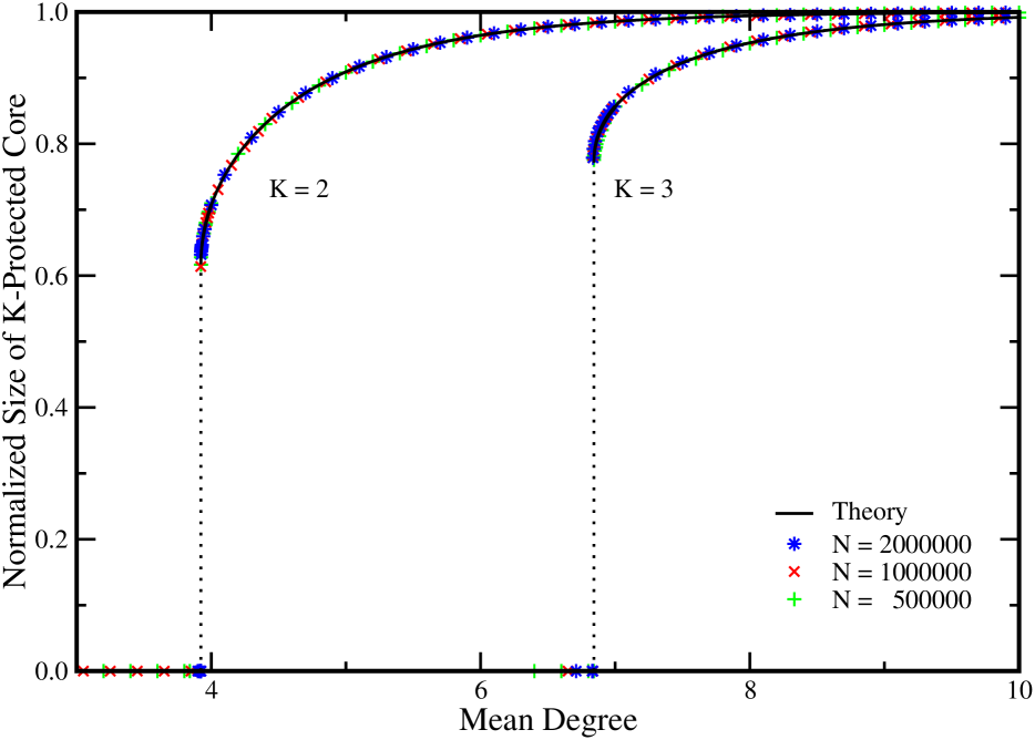
Figure 12: Normalized size of the $K$-protected core for the ER random network. The value of $K$ is set to $K=2$ or $K=3$. Symbols are simulation results on three network samples of size $N=5\times 10^{5}$, $10^{6}$, and $2\times 10^{6}$, respectively, while lines are theoretical predictions at $N=\infty$.

For ER random networks in the limit of $N\rightarrow+\infty$, the degree distribution is a Poisson distribution:

$$P(k)=\frac{e^{-c}c^{k}}{k!}\;,$$ (41)

where $c$ is the mean degree. The excess degree distribution $Q(k)$ is also a Poisson distribution:

$$Q(k)=\frac{e^{-c}c^{k-1}}{(k-1)!}\;,\quad\quad(k\geq 1)\;.$$ (42)

For the $2$-protected core percolation problem ($K=K^{\prime}=2$), the expressions for $\alpha$, $\beta$, $\gamma$, and $n_{\mathrm{p\mathchar 45\relax core}}$ are, respectively,

$$\alpha = e^{-c(1-\alpha-\beta-\gamma)}+e^{-c(1-\beta)}-e^{-c(1-\beta-\gamma)}\;,$$ (43)

$$\beta = 1+e^{-c(1-\beta-\gamma)}-e^{-c\alpha}-e^{-c(1-\alpha-\beta-\gamma)}\;,$$ (44)

$$\gamma = c(1-\alpha-\beta)e^{-c(1-\beta)}\;,$$ (45)

$$n_{\mathrm{p\mathchar 45\relax core}} = e^{-c\alpha}-e^{-c(1-\beta)}\bigl{[}1+c(1-\alpha-\beta)\bigr{]}\;.$$ (46)

The $2$-protected core percolation transition occurs at the critical mean degree $c^{*}\approx 3.9229$ (see Fig. 3 and Fig. 12).

For the $3$-protected core percolation problem ($K=K^{\prime}=3$), the expressions for $\alpha$, $\beta$, $\gamma$ and $n_{\mathrm{p\mathchar 45\relax core}}$ are, respectively,

$$\alpha = e^{-c(1-\alpha-\beta-\gamma)}\bigl{[}1+c(1-\alpha-\beta-\gamma)\bigr{]}+e^{-c(1-\beta)}\bigl{[}1+c(1-\alpha-\beta)\bigr{]}$$ (47)

$$\quad\quad-e^{-c(1-\beta-\gamma)}\bigl{[}1+c(1-\alpha-\beta-\gamma)\bigr{]}\;,$$

$$\beta = 1-e^{-c\alpha}-e^{-c(1-\alpha-\beta-\gamma)}\bigl{[}1+c(1-\alpha-\beta-\gamma)\bigr{]}$$ (48)

$$\quad\quad+e^{-c(1-\beta-\gamma)}\bigl{[}1+c(1-\alpha-\beta-\gamma)\bigr{]}\;,$$

$$\gamma = \frac{c^{2}(1-\alpha-\beta)^{2}}{2}e^{-c(1-\beta)}\;,$$ (49)

$$n_{\mathrm{p\mathchar 45\relax core}} = e^{-c\alpha}-e^{-c(1-\beta)}\bigl{[}1+c(1-\alpha-\beta)+\frac{c^{2}(1-\alpha-\beta)^{2}}{2}\bigr{]}\;.$$ (50)

The $3$-protected core percolation transition occurs at the critical mean degree $c^{*}\approx 6.8426$ (see Fig. 12).

Regular random (RR) networks

In a random regular network each node has exactly $k_{0}$ links. If $k_{0}\geq K$, the $K$-protected core will contain all the nodes in the network. We consider the situation of randomly deleting a fraction $\rho$ of the links. Then each node on average has $c=k_{0}(1-\rho)$ links. The degree distribution of the network is

$$P(k)=C_{k_{0}}^{k}(1-\rho)^{k}\rho^{(k_{0}-k)}\quad\quad(k\leq k_{0})\;,$$ (51)

while the excess degree distribution $Q(k)$ is given by

$$Q(k)=C_{k_{0}-1}^{k-1}(1-\rho)^{k-1}\rho^{(k_{0}-k)}\quad\quad(1\leq k\leq k_{0})\;.$$ (52)

For the $2$-protected core percolation problem, we have

$$\alpha = \bigl{[}\rho+(1-\rho)(\alpha+\beta+\gamma)\bigr{]}^{k_{0}-1}+\bigl{[}\rho+(1-\rho)\beta\bigr{]}^{k_{0}-1}-\bigl{[}\rho+(1-\rho)(\beta+\gamma)\bigr{]}^{k_{0}-1}\;,$$ (53)

$$\beta = 1-\bigl{[}\rho+(1-\rho)(1-\alpha)\bigr{]}^{k_{0}-1}-\bigl{[}\rho+(1-\rho)(\alpha+\beta+\gamma)\bigr{]}^{k_{0}-1}$$ (54)

$$\quad\quad+\bigl{[}\rho+(1-\rho)(\beta+\gamma)\bigr{]}^{k_{0}-1}\;,$$

$$\gamma = (1-\alpha-\beta)(1-\rho)(k_{0}-1)\bigl{[}\rho+(1-\rho)\beta\bigr{]}^{k_{0}-2}\;.$$ (55)

If each node has $k_{0}=4$ neighbours, then a phase transition occurs at $\rho\approx 0.2303$ (corresponding to critical mean degree $c^{*}\approx 3.0789$), at which the fraction of protected nodes jumps from $0$ to $n_{\mathrm{p\mathchar 45\relax core}}^{*}\approx 0.7725$. If each node has $k_{0}=6$ neighbours, the phase transition occurs at $\rho\approx 0.4380$ (corresponding to critical mean degree $c^{*}\approx 3.3721$), at which the normalized size of the $2$-protected core jumps from $0$ to $n_{\mathrm{p\mathchar 45\relax core}}^{*}\approx 0.7079$. The comparison between theory and simulations is shown in Fig. 5.

Random scale-free (SF) networks

Two types of random SF networks are considered in this work, namely purely SF networks and asymptotically SF networks.

Purely scale-free network with a minimal degree $k_{\rm min}$

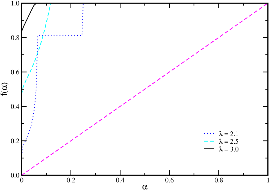
Figure 13: Function $f(\alpha)$ at $K=K^{\prime}=2$ for the purely SF random network. The minimal degree is $k_{\rm min}=1$ and the network size $N=\infty$. The degree exponent is set to $\lambda=2.1$ (dotted line), $2.5$ (dashed line) or $3.0$ (solid line). The equation $\alpha=f(\alpha)$ has only a single solution $\alpha=1$ for any degree exponent $\lambda>2$.

This type of SF networks is characterized by the degree distribution

$$P_{0}(k)=\frac{k^{-\lambda}}{\sum_{m\geq k_{\rm min}}m^{-\lambda}}\quad\quad(k\geq k_{\rm min})\;.$$ (56)

There are two control parameters, the degree exponent $\lambda$ and the minimal degree $k_{\rm min}$. If $\lambda\leq 2$, the mean degree of the network diverges in the thermodynamic limit of $N\rightarrow\infty$. We therefore assume that $\lambda>2$ hereafter. The minimal degree $k_{\rm min}\geq 1$. The excess degree distribution $Q_{0}(k)\equiv kP_{0}(k)/\sum_{k\geq k_{\rm min}}kP_{0}(k)$ is expressed as

$$Q_{0}(k)=\frac{k^{1-\lambda}}{\sum_{m\geq k_{\rm min}}m^{1-\lambda}}\;.$$ (57)

For the special case of $k_{\rm min}=1$, Fig. 13 shows the curve of $f(\alpha)$ at several different fixed $\lambda$ values. Because $\alpha=f(\alpha)$ has only a single solution $\alpha=1$, there is no $K$-protected core percolation transition in the system for all $K\geq 2$.

When $k_{\rm min}\geq K$, the whole network forms a $K$-protected core. If a randomly chosen fraction $\rho$ of the links are removed from the network, a $K$-protected core percolation transition occurs when the mean degree $c$ of the remaining network is decreased to certain threshold value $c^{*}$. After a fraction $\rho$ of the links are removed, the degree distribution $P(k)$ of the remaining network becomes

$$P(k)=\frac{1}{\sum_{m\geq k_{\rm min}}m^{-\lambda}}\sum\limits_{m\geq\max(k,k_{\rm min})}m^{-\lambda}C_{m}^{k}(1-\rho)^{k}\rho^{m-k}\;,$$ (58)

while the corresponding excess degree distribution $Q(k)$ is given by

$$Q(k)=\frac{1}{\sum_{m\geq k_{\rm min}}m^{1-\lambda}}\sum\limits_{m\geq\max(k,k_{\rm min})}m^{1-\lambda}C_{m-1}^{k-1}(1-\rho)^{k-1}\rho^{m-k}\;.\quad\quad(k\geq 1)$$ (59)

For the case of $K=2$, the expressions for the probabilities $\alpha$, $\beta$, and $\gamma$ are

$$\alpha = \frac{1}{\sum_{m\geq k_{\rm min}}m^{1-\lambda}}\sum\limits_{k\geq k_{\rm min}}k^{1-\lambda}\Bigl{[}\bigl{(}\rho+(1-\rho)(\alpha+\beta+\gamma)\bigr{)}^{k-1}+\bigl{(}\rho+(1-\rho)\beta\bigr{)}^{k-1}$$ (60)

$$\quad\quad\quad\quad\quad\quad\quad\quad\quad\quad\quad\quad\quad\quad-\bigl{(}\rho+(1-\rho)(\beta+\gamma)\bigr{)}^{k-1}\Bigr{]}\;,$$

$$\beta = 1-\frac{1}{\sum_{m\geq k_{\rm min}}m^{1-\lambda}}\sum\limits_{k\geq k_{\rm min}}k^{1-\lambda}\Bigl{[}\bigl{(}\rho+(1-\rho)(1-\alpha)\bigr{)}^{k-1}+\bigl{(}\rho+(1-\rho)(\alpha+\beta+\gamma)\bigr{)}^{k-1}$$ (61)

$$\quad\quad\quad\quad\quad\quad\quad\quad\quad\quad\quad\quad\quad\quad\quad\quad-\bigl{(}\rho+(1-\rho)(\beta+\gamma)\bigr{)}^{k-1}\Bigr{]}\;,$$

$$\gamma = \frac{(1-\alpha-\beta)(1-\rho)}{\sum_{m\geq k_{\rm min}}m^{1-\lambda}}\sum\limits_{k\geq k_{\rm min}}k^{1-\lambda}(k-1)\bigl{(}\rho+(1-\rho)\beta\bigr{)}^{k-2}\;.$$ (62)

And the normalized size of the $2$-protected core is

$$n_{\mathrm{p\mathchar 45\relax core}} = \frac{1}{\sum_{m\geq k_{\rm min}}m^{-\lambda}}\sum\limits_{k\geq k_{\rm min}}m^{-\lambda}\Bigl{[}\bigl{(}\rho+(1-\rho)(1-\alpha)\bigr{)}^{k}-\bigl{(}\rho+(1-\rho)\beta\bigr{)}^{k}$$ (63)

$$\quad\quad\quad\quad\quad-(1-\rho)(1-\alpha-\beta)k\bigl{(}\rho+(1-\rho)\beta\bigr{)}^{k-1}\Bigr{]}\;.$$

As long as $\lambda>2$, the summations in the above several equations converge even when the network size $N=\infty$.

For networks of finite size $N$, we generate a scale-free degree distribution as follows [46]: (0) Initialize an integer $n=0$ and initialize the degree to be $k=k_{\rm min}$, and initialize the candidate node set $U$ as containing all the $N$ nodes. (1) Set $n_{k}$ to be the integer that is closest to the real value $NP_{0}(k)$ (if $n_{k}=0$, then set $n_{k}=1$, and if $n+n_{k}>N$, then set $n_{k}=N-n$); perform the updating $n\leftarrow n+n_{k}$, and choose $n_{k}$ different nodes from the candidate set $U$ and assign the degree $k$ to each of them (and then remove these nodes from set $U$). (2) Set $k\leftarrow k+1$, and go back to step $(1)$ if $n<N$.

Through this construction, the degree distribution of the network is scale-free with a maximal degree $k_{\rm max}$, whose value scales with $N$ as $k_{\rm max}\approx k_{\rm min}N^{1/(\lambda-1)}$ [46].

After each node has been assigned a degree, we can construct a random SF network by the configuration model. Notice that when $\lambda<3$ there are intrinsic degree correlations in a random SF network [42, 43, 46, 47, 48, 49].

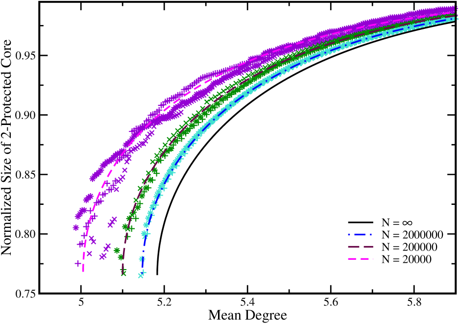
Figure 14: Normalized size of $2$-protected core for SF random networks with $\lambda=3$ and $k_{\rm min}=4$. A fraction $\rho$ of the links are randomly chosen and removed from the network. At each value of $N$, the line is theoretical prediction based on the degree distribution $P(k)$ while symbols are simulation results on three independent network instances with the same $P(k)$. The networks are obtained through the configuration model.

Some results on random SF networks with $\lambda=3$ and $k_{\rm min}=4$ are shown in Fig. 14. For $N\rightarrow\infty$, a $2$-protected core percolation transition occurs when the fraction of removed links $\rho\approx 0.2692$ (corresponding to critical mean degree $c^{*}\approx 5.1832$), with a jump of $n_{\mathrm{p\mathchar 45\relax core}}$ from $0$ to $n_{\mathrm{p\mathchar 45\relax core}}^{*}\approx 0.7655$. For finite networks, however, the theory predicts that the $2$-protected core actually is formed at much lower values of mean degree. For example, Fig. 14 demonstrates that, the critical degree is $c^{*}\approx 5.0052$ (for $N=2\times 10^{4}$), $c^{*}\approx 5.0999$ (for $N=2\times 10^{5}$), $c^{*}\approx 5.1465$ (for $N=2\times 10^{6}$), respectively. These predictions on finite-$N$ systems are confirmed by simulation results on single network instances.

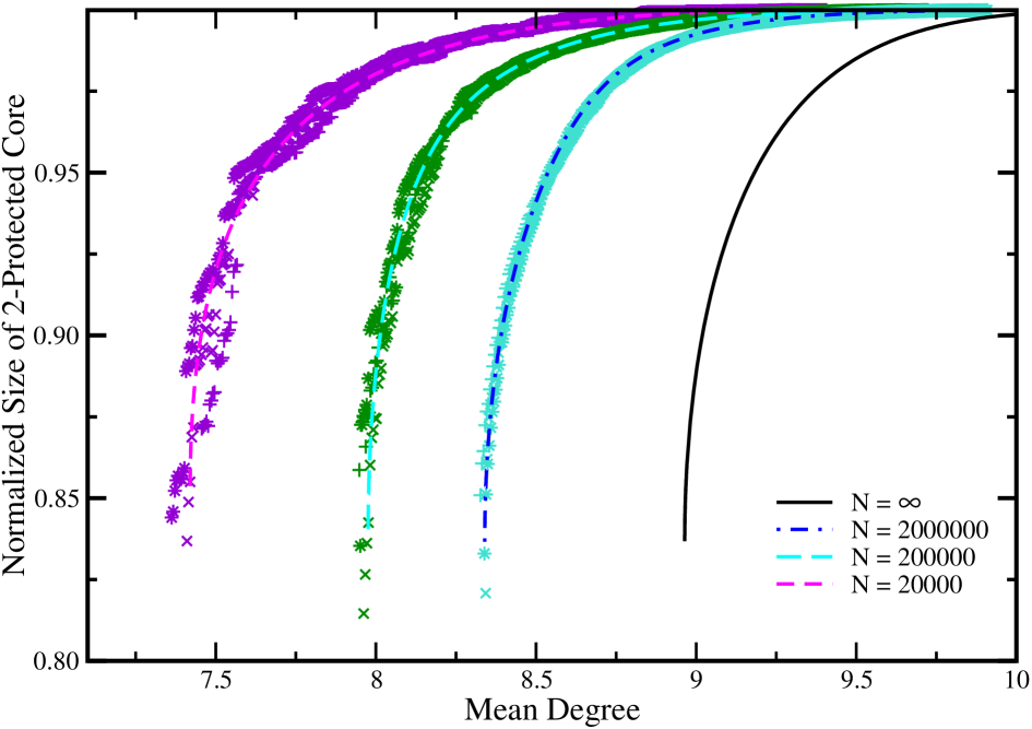
Figure 15: Normalized size of $2$-protected core for SF random networks with $\lambda=2.5$ and $k_{\rm min}=4$. A fraction $\rho$ of the links are randomly chosen and removed from the network. At each value of $N$, the line is theoretical prediction based on the degree distribution $P(k)$ while symbols are simulation results on three independent network instances with the same $P(k)$. The networks are obtained through the configuration model.

Figure 15 shows the comparison between theory and simulations on $2$-protected core percolation for random SF networks with minimal degree $k_{\rm min}=4$ and degree exponent $\lambda=2.5$. Similar to the results shown in Fig. 14, the $2$-protected core percolation transition is discontinuous, and there are also strong finite-size effects.

Static model

Random SF networks can also be constructed from the static model [41]. In the static model, each node $i\in\{1,2,\ldots,N\}$ has a weight $w_{i}=\frac{i^{-\xi}}{\sum_{j=1}^{N}j^{-\xi}}$, where $0\leq\xi<1$ is a control parameter. To create a link, two nodes $i$ and $j$ are chosen independently from the set of $N$ nodes, and the probability that node $i$ and node $j$ being chosen is equal to $w_{i}\times w_{j}$; if nodes $i$ and $j$ are different and the link $(i,j)$ has not been created before, then a link between $i$ and $j$ is set up. By repeating this connection process, a total number of $M=(c/2)N$ links are connected between pairs of nodes, with $c$ being the mean degree of the network. The resulting network has a scale-free degree distribution $P(k)\propto k^{-\lambda}$ for $k\gg 1$, with degree exponent $\lambda=1+1/\xi$ [41]. In the limit of $N\rightarrow\infty$, an analytic expression for $P(k)$ is given by [42]

$$P(k)=\frac{[c(1-\xi)]^{k}}{\xi\ k!}\int_{1}^{\infty}{\rm d}t\ e^{-c(1-\xi)t}t^{k-1-1/\xi}\;.$$ (64)

At $N\rightarrow\infty$ the excess degree distribution $Q(k)$ is given by

$$Q(k)=\Bigl{(}\frac{1}{\xi}-1\Bigr{)}\frac{[c(1-\xi)]^{k-1}}{(k-1)!}\int_{1}^{\infty}{\rm d}t\ e^{-c(1-\xi)t}t^{k-1-1/\xi}\;.$$ (65)

If we set $\xi=0$ in the static model we then obtain ER random networks. For $\xi<0.5$, the degree-degree correlations of neighbouring nodes in the network are negligible. But as $\xi$ increases from $0.5$ (therefore $\lambda$ is below $3.0$), the degree-degree correlations become more and more pronounced [42, 43].

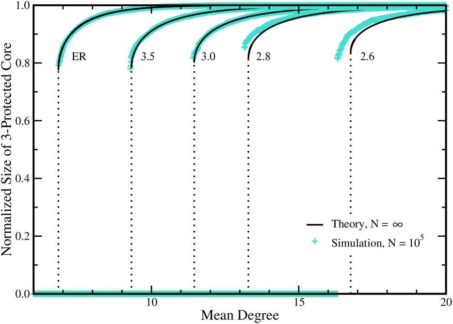
Figure 16: Normalized $3$-protected core size for ER networks and SF networks. The degree exponents of the SF networks are $\lambda=3.5,3.0,2.8,2.6$ (from left to right). Lines are analytic predictions for infinite system ($N=\infty$), while symbols are simulation results obtained on a single network instance with $N=10^{5}$ nodes. The SF and ER networks are all generated through the static model.

For the case of $K=2$, using Eq. (65) we obtain the follow expressions for $\alpha$, $\beta$, $\gamma$, and the normalized $2$-protected core size:

$$\alpha = \Bigl{(}\frac{1}{\xi}-1\Bigr{)}\Bigl{\{}E_{\frac{1}{\xi}}\bigl{[}c(1-\xi)(1-\alpha-\beta-\gamma)\bigr{]}+E_{\frac{1}{\xi}}\bigl{[}c(1-\xi)(1-\beta)\bigr{]}$$ (66)

$$\quad\quad\quad-E_{\frac{1}{\xi}}\bigl{[}c(1-\xi)(1-\beta-\gamma)\bigr{]}\Bigr{\}}\;,$$

$$\beta = 1-\Bigl{(}\frac{1}{\xi}-1\Bigr{)}\Bigl{\{}E_{\frac{1}{\xi}}\bigl{[}c(1-\xi)\alpha\bigr{]}+E_{\frac{1}{\xi}}\bigl{[}c(1-\xi)(1-\alpha-\beta-\gamma)\bigr{]}$$ (67)

$$\quad\quad\quad\quad-E_{\frac{1}{\xi}}\bigl{[}c(1-\xi)(1-\beta-\gamma)\bigr{]}\Bigr{\}}\;,$$

$$\gamma = \frac{(1-\alpha-\beta)c(1-\xi)^{2}}{\xi}E_{\frac{1-\xi}{\xi}}\bigl{[}c(1-\xi)(1-\beta)\bigr{]}\;,$$ (68)

$$n_{\mathrm{p\mathchar 45\relax core}} = \frac{1}{\xi}E_{\frac{1+\xi}{\xi}}\bigl{[}c(1-\xi)\alpha\bigr{]}-\frac{1}{\xi}E_{\frac{1+\xi}{\xi}}\bigl{[}c(1-\xi)(1-\beta)\bigr{]}$$ (69)

$$\quad\quad\quad-\frac{c(1-\xi)(1-\alpha-\beta)}{\xi}E_{\frac{1}{\xi}}\bigl{[}c(1-\xi)(1-\beta)\bigr{]}\;.$$

In the above equations, $E_{a}(x)$ is the generalized exponential integral defined as $E_{a}(x)\equiv\int_{1}^{\infty}{\rm d}te^{-xt}t^{-a}$. In the numerical calculations, the value of $E_{a}(x)$ is calculated by converting it into an incomplete gamma function and then using the GNU Scientific Library (gsl, http://www.gnu.org/software/gsl/).

For the case of $K=3$, the explicit expressions for $\alpha$, $\beta$, $\gamma$, and $n_{\mathrm{p\mathchar 45\relax core}}$ are, respectively,

$$\alpha = \Bigl{(}\frac{1}{\xi}-1\Bigr{)}\Bigl{\{}E_{\frac{1}{\xi}}\bigl{[}c(1-\xi)(1-\alpha-\beta-\gamma)\bigr{]}+E_{\frac{1}{\xi}}\bigl{[}c(1-\xi)(1-\beta)\bigr{]}$$ (70)

$$\quad\quad-E_{\frac{1}{\xi}}\bigl{[}c(1-\xi)(1-\beta-\gamma)\bigr{]}\Bigr{\}}+\frac{(1-\alpha-\beta)c(1-\xi)^{2}}{\xi}E_{\frac{1-\xi}{\xi}}\bigl{[}c(1-\xi)(1-\beta)\bigr{]}$$

$$+\frac{(1-\alpha-\beta-\gamma)c(1-\xi)^{2}}{\xi}\Bigl{\{}E_{\frac{1-\xi}{\xi}}\bigl{[}c(1-\xi)(1-\alpha-\beta-\gamma)\bigr{]}$$

$$\quad\quad\quad\quad\quad\quad\quad\quad\quad\quad\quad\quad\quad\quad-E_{\frac{1-\xi}{\xi}}\bigl{[}c(1-\xi)(1-\beta-\gamma)\bigr{]}\Bigr{\}}\;,$$

$$\beta = 1-\Bigl{(}\frac{1}{\xi}-1\Bigr{)}\Bigl{\{}E_{\frac{1}{\xi}}\bigl{[}c(1-\xi)\alpha\bigr{]}+E_{\frac{1}{\xi}}\bigl{[}c(1-\xi)(1-\alpha-\beta-\gamma)\bigr{]}-E_{\frac{1}{\xi}}\bigl{[}c(1-\xi)(1-\beta-\gamma)\bigr{]}\Bigr{\}}$$ (71)

$$-\frac{(1-\alpha-\beta-\gamma)c(1-\xi)^{2}}{\xi}\Bigl{\{}E_{\frac{1-\xi}{\xi}}\bigl{[}c(1-\xi)(1-\alpha-\beta-\gamma)\bigr{]}$$

$$\quad\quad\quad\quad\quad\quad\quad\quad\quad\quad\quad\quad\quad\quad-E_{\frac{1-\xi}{\xi}}\bigl{[}c(1-\xi)(1-\beta-\gamma)\bigr{]}\Bigr{\}}\;,$$

$$\gamma = \frac{(1-\alpha-\beta)^{2}c^{2}(1-\xi)^{3}}{2\xi}E_{\frac{1-2\xi}{\xi}}\bigl{[}c(1-\xi)(1-\beta)\bigr{]}\;,$$ (72)

$$n_{\mathrm{p\mathchar 45\relax core}} = \frac{1}{\xi}\Bigl{\{}E_{\frac{1+\xi}{\xi}}\bigl{[}c(1-\xi)\alpha\bigr{]}-E_{\frac{1+\xi}{\xi}}\bigl{[}c(1-\xi)(1-\beta)\bigr{]}\Bigr{\}}-\frac{(1-\alpha-\beta)c(1-\xi)}{\xi}E_{\frac{1}{\xi}}\bigl{[}c(1-\xi)(1-\beta)\bigr{]}$$ (73)

$$-\frac{(1-\alpha-\beta)^{2}c^{2}(1-\xi)^{2}}{2\xi}E_{\frac{1-\xi}{\xi}}\bigl{[}c(1-\xi)(1-\beta)\bigr{]}\;.$$

Figure 16 shows additional numerical results on the normalized $3$-projected core size for SF networks generated through the static model.

Supplementary note 8

We offer more details on the numerical simulations in lattice systems.

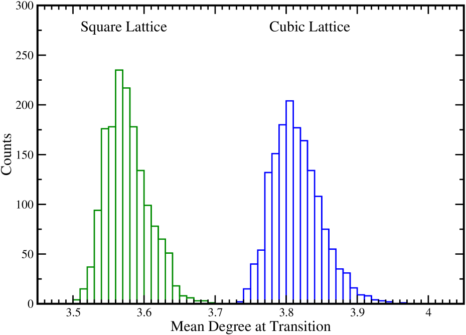
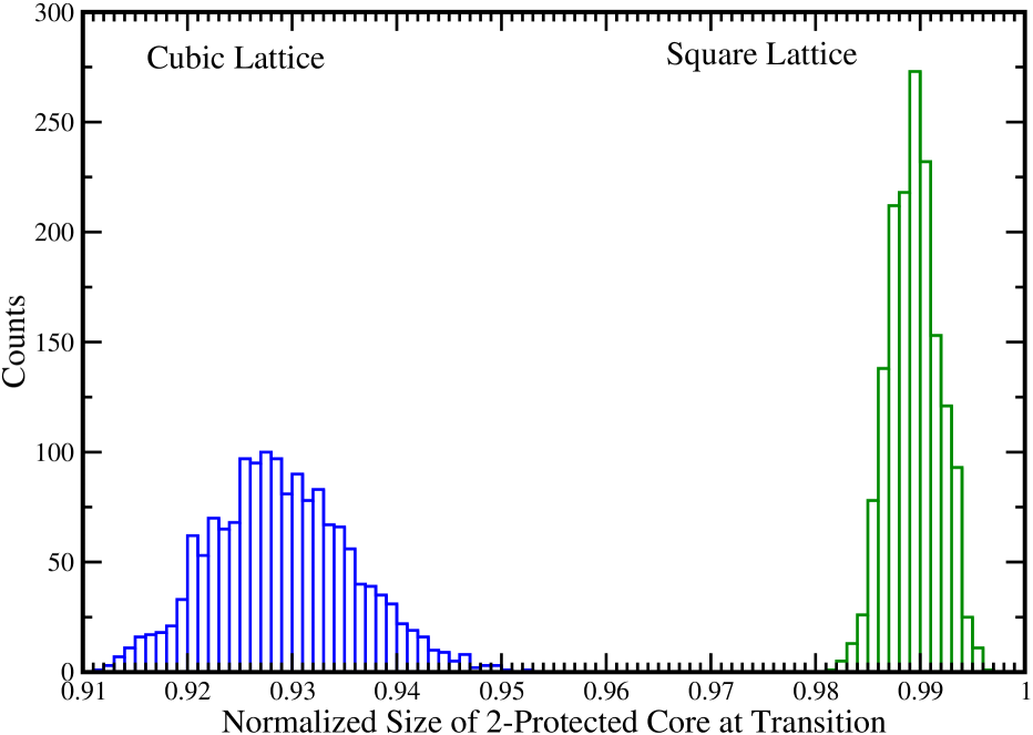
Figure 17: Fluctuations of the $2$-protected core percolation transition point in 2D square lattice and 3D cubic lattice. Histograms of mean network degree $c^{*}$ (a) and normalized sizes of the $2$-protected core $n_{p-core}^{*}$ (b) at the transition point are obtained by simulations on $1600$ independent network instances of the 2D periodic square lattice and the 3D periodic cubic lattice of size $N=10^{6}$.

We consider $D$-dimensional hypercubic lattices of side length $L$ and periodic boundary conditions. The total number of nodes in the lattice is $N=L^{D}$, and each node has $k_{0}=2D$ links. After a randomly chosen fraction $\rho$ of the links are deleted from the network, the degree distribution $P(k)$ and the excess degree distribution $Q(k)$ of the remaining network are described by Eq. (51) and Eq. (52), respectively. Therefore the theoretical predictions of $K$-protected core percolation in the lattice systems are identical to those of the random regular network systems.

Some simulation results for the $D=2$ (side length $L=1000$) and $D=3$ (side length $L=100$) lattices are described in Fig. 5. Our mean field theory correctly predicts the normalized $2$-protected core size once the percolation transition occurs, but it fails to predict the transition point. With a given value of $N$, the $2$-protected core percolation transition points $c^{*}$ actually fluctuate considerably among different network instances (obtained by removing a randomly chosen subset of the whole links). Figure 17 shows the fluctuations of the value of $c^{*}$ among $1600$ independent network instances with $N=10^{6}$ nodes, and the associated fluctuations of the normalized $2$-protected core sizes $n_{\rm p-core}^{*}$.

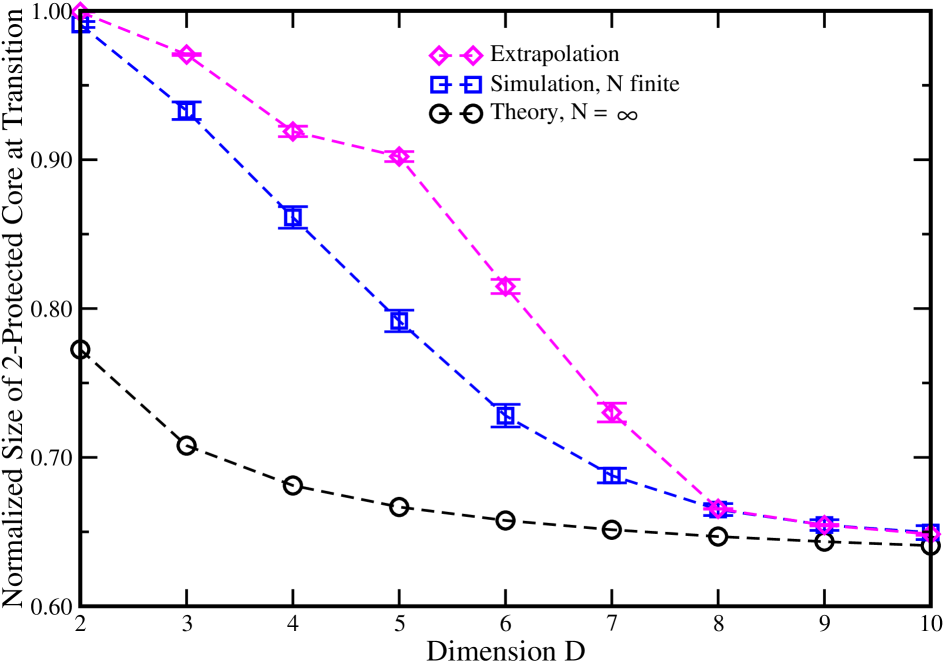
Figure 18: The normalized size of the $2$-protected core at the transition point in $D$-dimensional hypercubic lattices. Each node of the network originally has $k_{0}=2D$ neighbours. A randomly chosen fraction $\rho$ of the links are deleted from the network. The lattice data (squares) were obtained by simulating on $1600$ independent network instances (the number of nodes in the networks is $N=L^{D}$, with $L=1414,126,38,18,11,8,6,5,4$ for $D=2$ to $D=10$, respectively); the diamond symbols are the extrapolated simulation value in the $N\rightarrow\infty$ limit. The theoretical predictions (circle symbols) on the $2$-protected core percolation transition point for infinite large system ($N=\infty$) are obtained by using Eqs. (51)–(55).

The mean value $\overline{c^{*}}$ of the $2$-protected core percolation transition point $c^{*}$ is obtained by averaging over $1600$ independent network instances. The value of $\overline{c^{*}}$ changes with network size $N$ for $D\leq 7$ (see Figs. 19–25 for the dimensions from $D=2$ to $D=8$). For $D\leq 8$, it appears that $\overline{c^{*}}$ approaches a limiting value $c^{*}_{\infty}$ as follows

$$\overline{c^{*}}=c^{*}_{\infty}-\frac{a}{\ln N}\;,$$ (74)

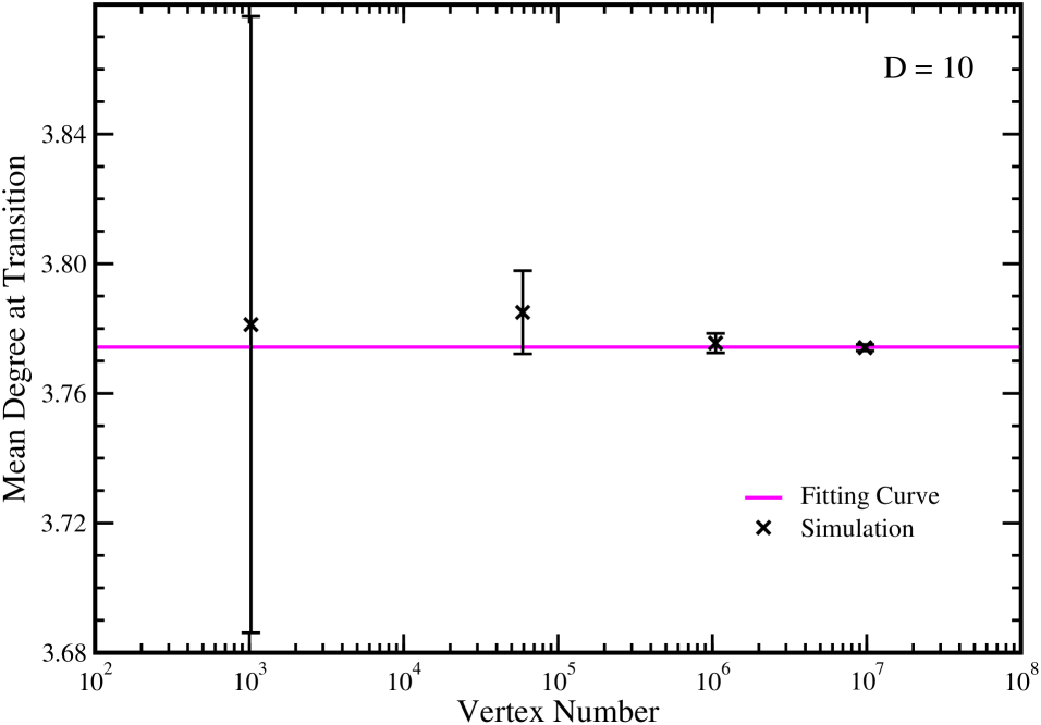
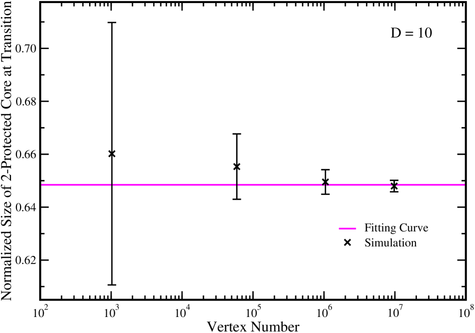
Figure 27: Extrapolation of $2$-protected core percolation transition point to the $N\rightarrow+\infty$ limit for $10$-dimensional hypercubic lattices. (a) Average value $\overline{c^{*}}$ of the mean degree $c^{*}$ at the $2$-protected core transition. (b) Average value $\overline{n_{\rm p-core}^{*}}$ of the normalized $2$-protected core size $n_{\rm p-core}^{*}$ at the percolation transition. Each data point is obtained by averaging over $1600$ independent network instances. The fitting cure is $y=a_{1}$, with $a_{1}=3.7743\pm 0.0005$ (a) and $y=a_{2}$ with $a_{2}=0.6484\pm 0.0008$ (b).

where $a$ is a dimension-dependent constant. From the above fitting formula we obtain the value of $c^{*}_{\infty}$ in the thermodynamic limit $N\rightarrow\infty$. As shown in Fig. 6, the value of $c^{*}_{\infty}$ is markedly different from the mean value $\overline{c^{*}}$ of finite systems with $N\approx 2\times 10^{6}$, especially for dimension $D\leq 6$. For $D\geq 9$ the average value of the $2$-protected core transition point $c^{*}$ does not change much with system size $N$ (see Fig. 26 and Fig. 27). When $D\rightarrow\infty$, we expect the behaviors of the lattice systems to be the same as the random regular networks.

We also extrapolate the average values of $n_{\rm p-core}^{*}$ at the $2$-protected core percolation transition point to $N\rightarrow\infty$, see Figs. 19–27. As shown in Fig. 18, finite-size effects are most significant for $D=2,3$. As $D$ increases the results obtained from the finite-dimensional lattice systems become more and more closer to the theoretical predictions obtained from random regular networks.

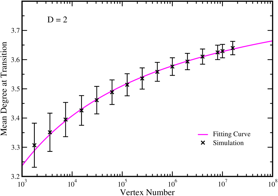
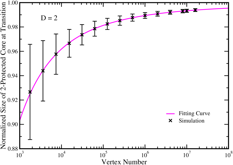
Figure 19: Extrapolation of $2$-protected core percolation transition point to the $N\rightarrow\infty$ limit for square lattices. (a) Average value $\overline{c^{*}}$ of the mean degree $c^{*}$ at the $2$-protected core transition. (b) Average value $\overline{n_{\rm p-core}^{*}}$ of the normalized $2$-protected core size $n_{\rm p-core}^{*}$ at the percolation transition. Each data point is obtained by averaging over $1600$ independent network instances. The fitting cure is $y=a_{1}-b_{1}/\ln(x)$, with $a_{1}=3.921\pm 0.005$ and $b_{1}=4.73\pm 0.06$ (a) and $y=a_{2}-b_{2}/\ln^{\eta}(x)$ with $a_{2}=0.9993\pm 0.0001$, $b_{2}=54.6\pm 3.6$, $\eta=3.28\pm 0.03$ (b). The fitting parameters $a_{1}$ and $a_{2}$ are regarded as the value of $c^{*}$ and the value of $n_{\rm p-core}^{*}$ in the $N\rightarrow\infty$ system (they are shown in Fig. 6 and Fig. 18).

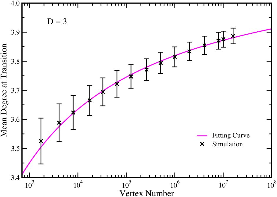
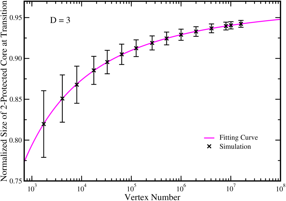
Figure 20: Extrapolation of $2$-protected core percolation transition point to the $N\rightarrow\infty$ limit for cubic lattices. (a) Average value $\overline{c^{*}}$ of the mean degree $c^{*}$ at the $2$-protected core transition. (b) Average value $\overline{n_{\rm p-core}^{*}}$ of the normalized $2$-protected core size $n_{\rm p-core}^{*}$ at the percolation transition. Each data point is obtained by averaging over $1600$ independent network instances. The fitting cure is $y=a_{1}-b_{1}/\ln(x)$, with $a_{1}=4.188\pm 0.007$ and $b_{1}=5.1\pm 0.1$ (a) and $y=a_{2}-b_{2}/\ln^{\eta}(x)$ with $a_{2}=0.9707\pm 0.0006$, $b_{2}=9.99\pm 0.47$, $\eta=2.09\pm 0.02$ (b).

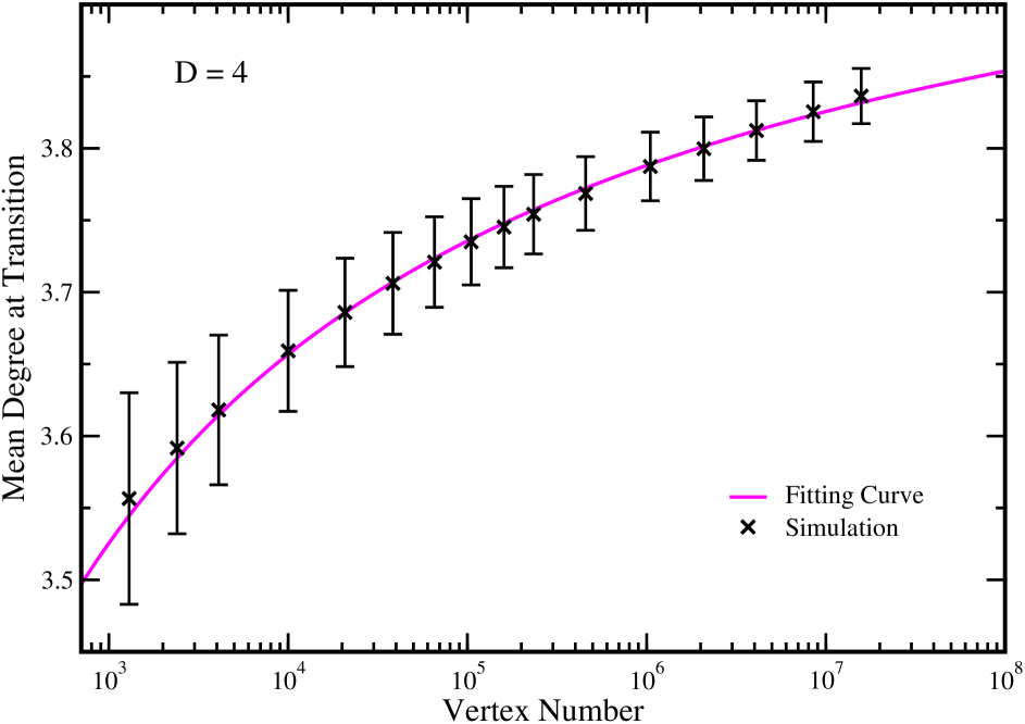
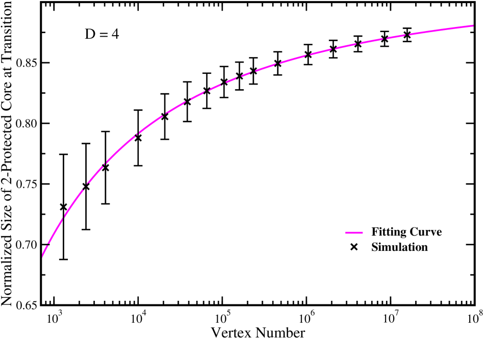
Figure 21: Extrapolation of $2$-protected core percolation transition point to the $N\rightarrow\infty$ limit for $4$-dimensional hypercubic lattices. (a) Average value $\overline{c^{*}}$ of the mean degree $c^{*}$ at the $2$-protected core transition. (b) Average value $\overline{n_{\rm p-core}^{*}}$ of the normalized $2$-protected core size $n_{\rm p-core}^{*}$ at the percolation transition. Each data point is obtained by averaging over $1600$ independent network instances. The fitting cure is $y=a_{1}-b_{1}/\ln(x)$, with $a_{1}=4.051\pm 0.004$ and $b_{1}=3.63\pm 0.05$ (a) and $y=a_{2}-b_{2}/\ln^{\eta}(x)$ with $a_{2}=0.919\pm 0.004$, $b_{2}=6.0\pm 0.9$, $\eta=1.74\pm 0.08$ (b).

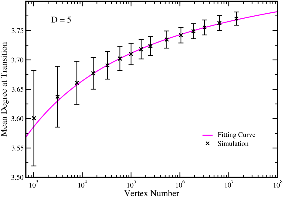
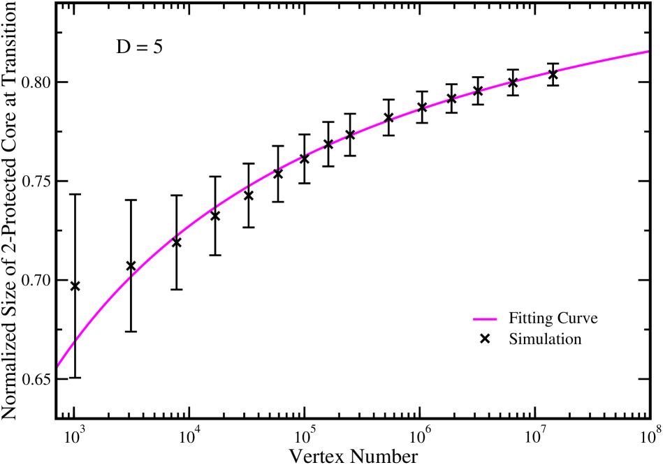
Figure 22: Extrapolation of $2$-protected core percolation transition point to the $N\rightarrow\infty$ limit for $5$-dimensional hypercubic lattices. (a) Average value $\overline{c^{*}}$ of the mean degree $c^{*}$ at the $2$-protected core transition. (b) Average value $\overline{n_{\rm p-core}^{*}}$ of the normalized $2$-protected core size $n_{\rm p-core}^{*}$ at the percolation transition. Each data point is obtained by averaging over $1600$ independent network instances. The fitting cure is $y=a_{1}-b_{1}/\ln(x)$, with $a_{1}=3.900\pm 0.003$ and $b_{1}=2.17\pm 0.03$ (a) and $y=a_{2}-b_{2}/\ln(x)$ with $a_{2}=0.902\pm 0.003$, $b_{2}=1.61\pm 0.05$ (b).

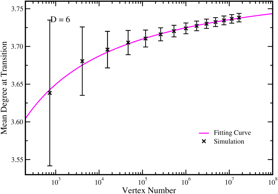
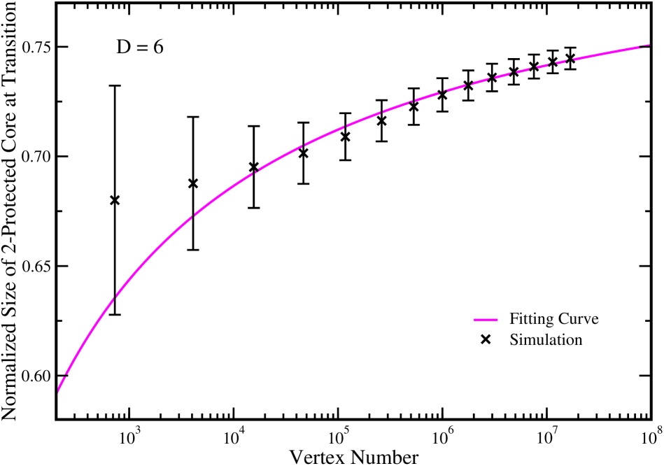
Figure 23: Extrapolation of $2$-protected core percolation transition point to the $N\rightarrow\infty$ limit for $6$-dimensional hypercubic lattices. (a) Average value $\overline{c^{*}}$ of the mean degree $c^{*}$ at the $2$-protected core transition. (b) Average value $\overline{n_{\rm p-core}^{*}}$ of the normalized $2$-protected core size $n_{\rm p-core}^{*}$ at the percolation transition. Each data point is obtained by averaging over $1600$ independent network instances. The fitting cure is $y=a_{1}-b_{1}/\ln(x)$, with $a_{1}=3.800\pm 0.002$ and $b_{1}=1.04\pm 0.02$ (a) and $y=a_{2}-b_{2}/\ln(x)$ with $a_{2}=0.815\pm 0.005$, $b_{2}=1.18\pm 0.07$ (b).

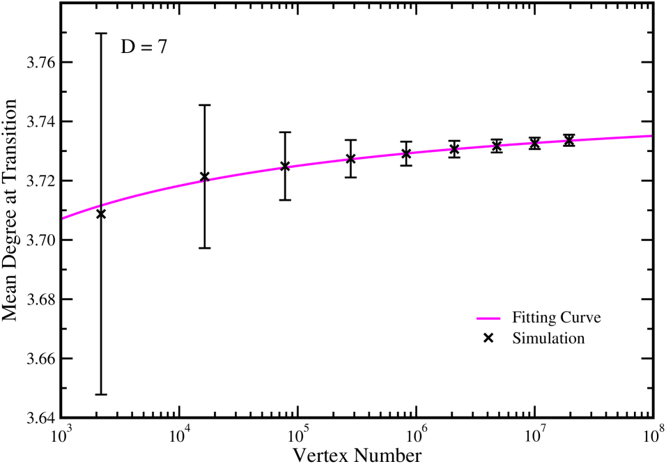
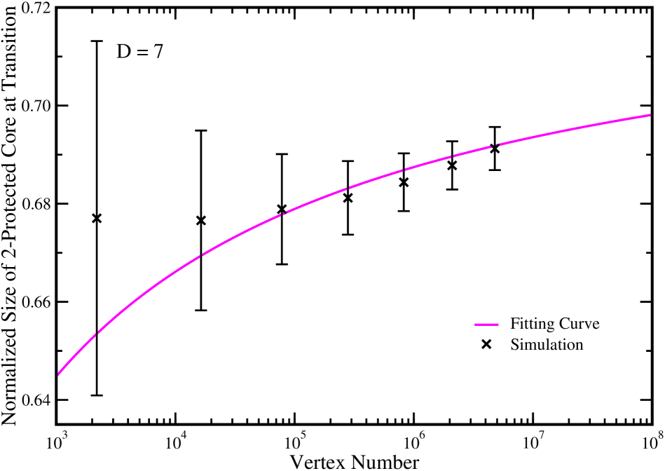
Figure 24: Extrapolation of $2$-protected core percolation transition point to the $N\rightarrow\infty$ limit for $7$-dimensional hypercubic lattices. (a) Average value $\overline{c^{*}}$ of the mean degree $c^{*}$ at the $2$-protected core transition. (b) Average value $\overline{n_{\rm p-core}^{*}}$ of the normalized $2$-protected core size $n_{\rm p-core}^{*}$ at the percolation transition. Each data point is obtained by averaging over $1600$ independent network instances. The fitting cure is $y=a_{1}-b_{1}/\ln(x)$, with $a_{1}=3.75197\pm 0.0006$ and $b_{1}=0.3104\pm 0.0098$ (a) and $y=a_{2}-b_{2}/\ln(x)$ with $a_{2}=0.730\pm 0.006$, $b_{2}=0.59\pm 0.09$ (b).

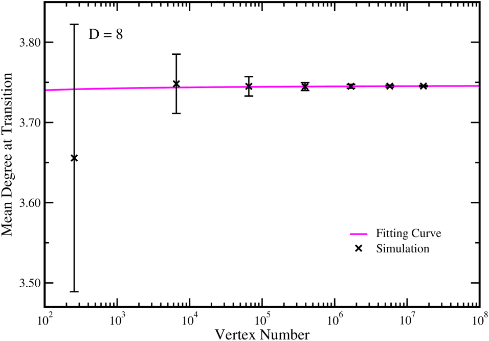
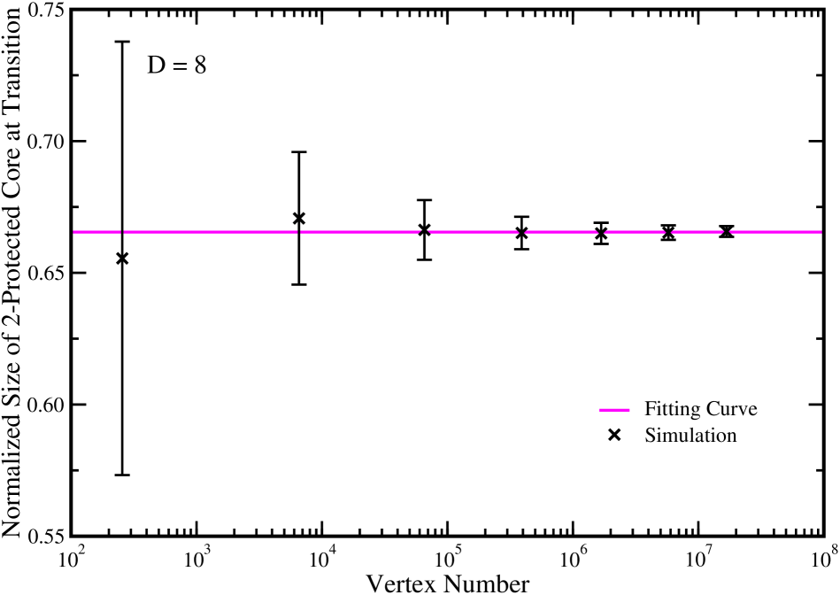
Figure 25: Extrapolation of $2$-protected core percolation transition point to the $N\rightarrow+\infty$ limit for $8$-dimensional hypercubic lattices. (a) Average value $\overline{c^{*}}$ of the mean degree $c^{*}$ at the $2$-protected core transition. (b) Average value $\overline{n_{\rm p-core}^{*}}$ of the normalized $2$-protected core size $n_{\rm p-core}^{*}$ at the percolation transition. Each data point is obtained by averaging over $1600$ independent network instances. The fitting cure is $y=a_{1}-b_{1}/\ln(x)$, with $a_{1}=3.747\pm 0.002$ and $b_{1}=0.03\pm 0.04$ (a) and $y=a_{2}$ with $a_{2}=0.6655\pm 0.0002$ (b).

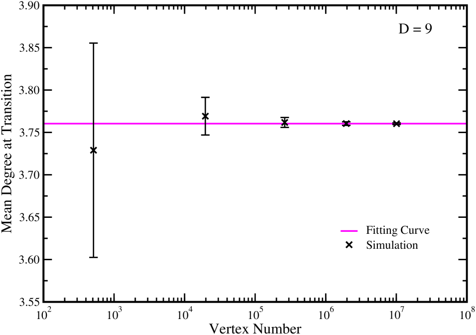
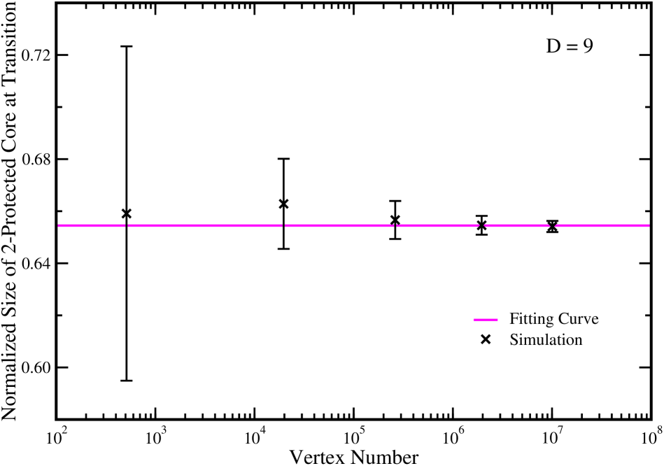
Figure 26: Extrapolation of $2$-protected core percolation transition point to the $N\rightarrow\infty$ limit for $9$-dimensional hypercubic lattices. (a) Average value $\overline{c^{*}}$ of the mean degree $c^{*}$ at the $2$-protected core transition. (b) Average value $\overline{n_{\rm p-core}^{*}}$ of the normalized $2$-protected core size $n_{\rm p-core}^{*}$ at the percolation transition. Each data point is obtained by averaging over $1600$ independent network instances. The fitting cure is $y=a_{1}$, with $a_{1}=3.7604\pm 0.0002$ (a) and $y=a_{2}$ with $a_{2}=0.6545\pm 0.0005$ (b).

Supplementary Note 9

We test the performance of the mean-field theory on a set of $37$ real-world networks listed in Tab. 1. As shown in Tab. 2, the normalized $2$-protected core sizes $n_{\mathrm{p\mathchar 45\relax core}}$ calculated from the theory are in good agreement with the empirical results for $32$ of the networks. Such a good performance is rather surprising to us, since our mean field theory only uses the degree distribution $P(k)$ as input and it completely ignores all the possible higher order correlations (e.g., degree-degree correlation, clustering, modularity, etc.) in real-world networks.

We also realize that the mean-field theory does not perform very well for metabolic networks and world-wide web (WWW). In one data set (the network of hyperlinks between weblogs on politics [67], our theory predicts large $2$-protected core size, while the real network does not have a $2$-protected core at all. In other four cases (two WWW domain networks [57, 66] and two metabolic networks [63]), the theory predicts zero $2$-protected core size. Yet, these real-world networks do have $2$-protected cores containing $20\%-75\%$ of the nodes.

The above findings raise a fundamental question: Beside the degree distribution of the network, which other network characteristics also have significant influences to the size of the protected core? Addressing this and other related questions deserves a systematic study and we leave it as future work.

Supplementary References

1. Sinclair, A. Algorithms for Random Generation and Counting: a Markov Chain Approach (Birkhäuser, Boston, MA, 1993).

2. Zhou, H. J. & Lipowsky, R. Dynamic pattern evolution on scale-free networks. Proc. Natl. Acad. Sci. USA 102, 10052–10057 (2005).

3. Zhou, H. J. & Lipowsky, R. Activity patterns on random scale-free networks: global dynamics arising from local majority rules. J. Stat. Mech.: Theor. Exp. P01009 (2007).

4. King, O. D. Comment on ”subgraphs in random networks”. Phys. Rev. E 70, 058101 (2004).

5. Klein-Hennig, H. & Hartmann, A. K. Bias in generation of random graphs. Phys. Rev. E 85, 026101 (2012).

6. Bauke, H. & Mertens, S. Random numbers for large-scale distributed monte carlo simulations. Phys. Rev. E 75, 066701 (2007).

7. Balaji, S., Babu, M. M., Iyer, L. M., Luscombe, N. M. & Aravind, L. Comprehensive analysis of combinatorial regulation using the transcriptional regulatory network of yeast. J. Mol. Biol. 360, 213–227 (2006).

8. Milo, R. et al. Network motifs: Simple building blocks of complex networks. Science 298, 824–827 (2002).

9. Gama-Castro, S. et al. Regulondb (version 6.0): gene regulation model of escherichia coli k-12 beyond transcription, active (experimental) annotated promoters and textpresso navigation. Nucleic Acids Res. 36, D120–124 (2008).

10. Norlen, K., Lucas, G., Gebbie, M. & Chuang, J. Eva: Extraction, visualization and analysis of the telecommunications and media ownership network. In Proceedings of International Telecommunications Society 14th Biennial Conference (Seoul, Korea, 2002).

11. van Duijn, M. A. J., Zeggelink, E. P. H., Huisman, M., Stokman, F. N. & Wasseur, F. W. Evolution of sociology freshmen into a friendship network. J. Math. Sociol. 27, 153–191 (2003).

12. Milo, R. et al. Superfamilies of evolved and designed networks. Science 503, 1538–1542 (2004).

13. Leskovec, J., Lang, K. J., Dasgupta, A. & Mahoney, M. W. Community structure in large networks: Natural cluster sizes and the absence of large well-defined clusters. arXiv:0810.1355 (2008).

14. Richardson, M., Agrawal, R. & Domingos, P. Trust management for the semantic web. Lect. Notes Comput. Sci. 2870, 351–368 (2003).

15. Dunne, J. A., Williams, R. J. & Martinez, N. D. Food-web structure and network theory: The role of connectance and size. Proc. Natl. Acad. Sci. USA 99, 12917–12922 (2002).

16. Martinez, N. D. Artifacts or attributes? effects of resolution on the little rock lake food web. Ecol. Monographs 61, 367–392 (1991).

17. Christian, R. R. & Luczkovich, J. J. Organizing and understanding a winter’s seagrass foodweb network through effective trophic levels. Ecol. Modelling 117, 99–124 (1999).

18. Bianconi, G., Gulbahce, N. & Motter, A. E. Local structure of directed networks. Phys. Rev. Lett. 100, 118701 (2008).

19. Jeong, H., Tombor, B., Albert, R., Oltvai, Z. N. & Barabási, A.-L. The large-scale organization of metabolic networks. Nature 407, 651–654 (2000).

20. Watts, D. J. & Strogatz, S. H. Collective dynamics of ’small-world’ netowrks. Nature 393, 440–442 (1998).

21. Leskovec, J., Kleinberg, J. & Faloutsos, C. Graphs over time: densification laws, shrinking diameters and possible explanations. In Proceedings of the eleventh ACM SIGKDD international conference on Knowledge discovery in data mining, 177–187 (ACM, New York, 2005).

22. Albert, R., Jeong, H. & Barabási, A.-L. Internet: Diameter of the world-wide web. Nature 401, 130–131 (1999).

23. Adamic, L. A. & Glance, N. The political blogosphere and the 2004 u.s. election: divided they blog. In Proceedings of the 3rd international workshop on Link discovery, 36–43 (ACM, New York, 2005).

24. Leskovec, J., Kleinberg, J. & Faloutsos, C. Graph evolution: Densification and shrinking diameters. ACM Transactions on Knowledge Discovery from Data 1, 2 (2007).

25. Opsahl, T. & Panzarasa, P. Clustering in weighted networks. Social Networks 31, 155–163 (2009).

26. Eckmann, J.-P., Moses, E. & Sergi, D. Entropy of dialogues creates coherent structures in e-mail traffic. Proc. Natl. Acad. Sci. USA 101, 14333–14337 (2004).

27. Song, C., Qu, Z., Blumm, N. & Barabási, A.-L. Limits of predictability in human mobility. Science 327, 1018–1021 (2010).

28. Freeman, S. & Freeman, L. Social Science Research Reports 46 (University of California, Irvine, CA) (1979).

29. Cross, R. & Parker, A. The Hidden Power of Social Networks (Harvard Business School Press, Boston, MA, 2004).

References

- (1) Stauffer, D. & Aharony, A. Introduction to percolation theory (CRC Press, Boca Raton, Florida, 1994), 2 edn.
- (2) Dorogovtsev, S. N., Goltsev, A. V. & Mendes, J. F. F. Critical phenomena in complex networks. Rev. Mod. Phys. 80, 1275–1335 (2008).
- (3) Buldyrev, S. V., Parshani, R., Paul, G., Stanley, H. E. & Havlin, S. Catastrophic cascade of failures in interdependent networks. Nature 464, 1025–1028 (2010).
- (4) Albert, R., Jeong, H. & Barabási, A.-L. Error and attack tolerance of complex networks. Nature 406, 378–382 (2000).
- (5) Cohen, R., Erez, K., ben-Avraham, D. & Havlin, S. Resilience of the internet to random breakdowns. Phys. Rev. Lett. 85, 4626–4628 (2000).
- (6) Watts, D. J. A simple model of global cascades on random networks. Proc. Natl. Acad. Sci. USA 99, 5766–5771 (2002).
- (7) Li, W., Bashan, A., Buldyrev, S., Stanley, H. E. & Havlin, S. Cascading failures in interdependent lattice networks: The critical role of the length of dependency links. Phys. Rev. Lett. 108, 228702 (2012).
- (8) Pastor-Satorras, R. & Vespignani, A. Epidemic spreading in scale-free networks. Phys. Rev. Lett. 86, 3200–3203 (2001).
- (9) Kitsak, M. et al. Identification of influential spreaders in complex networks. Nature Phys. 6, 888–893 (2010).
- (10) Gleeson, J. P. High-accuracy approximation of binary-state dynamics on networks. Phys. Rev. Lett. 107, 068701 (2011).
- (11) Liu, Y.-Y., Slotine, J.-J. & Barabási, A.-L. Controllability of complex networks. Nature 473, 167–173 (2011).
- (12) Liu, Y.-Y., Csóka, E., Zhou, H. J. & Pósfai, M. Core percolation on complex networks. Phys. Rev. Lett. 109, 205703 (2012).
- (13) Erdös, P. & Rényi, A. On the evolution of random graphs. Publ. Math. Inst. Hung. Acad. Sci. 5, 17–60 (1960).
- (14) Callaway, D. S., Newman, M. E. J., Strogatz, S. H. & Watts, D. J. Network robustness and fragility: Percolation on random graphs. Phys. Rev. Lett. 85, 5468–5471 (2000).
- (15) Bollobás, B. Random Graphs (Cambridge University Press, Cambridge, UK, 2001), 2nd edn.
- (16) Achlioptas, D., D’Souza, R. M. & Spencer, J. Explosive percolation in random networks. Science 323, 1453–1455 (2009).
- (17) Riordan, O. & Warnke, L. Explosive percolation is continuous. Science 333, 322–324 (2011).
- (18) Nagler, J., Levina, A. & Timme, M. Impact of single links in competitive percolation. Nature Phys. 7, 265–270 (2011).
- (19) Nagler, J., Tiessen, T. & Gutch, H. W. Continuous percolation with discontinuities. Phys. Rev. X 2, 031009 (2012).
- (20) Boettcher, S., Singh, V. & Ziff, R. M. Ordinary percolation with discontinuous transitions. Nature Communications 3, 787 (2012).
- (21) Cho, Y. S., Hwang, S., Herrmann, H. J. & Kahng, B. Avoiding a spanning cluster in percolation models. Science 339, 1185–1187 (2013).
- (22) Chalupa, J., Leath, P. L. & Reich, G. R. Bootstrap percolation on a bethe lattice. J. Phys. C: Solid State Phys. 12, L31–L35 (1979).
- (23) Pittel, B., Spencer, J. & Wormald, N. Sudden emergence of a giant -core in a random graph. J. Combin. Theory B 67, 111–151 (1996).
- (24) Dorogovtsev, S. N., Goltsev, A. V. & Mendes, J. F. F. k-core organization of complex networks. Phys. Rev. Lett. 96, 040601 (2006).
- (25) Baxter, G. J., Dorogovtsev, S. N., Goltsev, A. V. & Mendes, J. F. F. Bootstrap percolation on complex networks. Phys. Rev. E 82, 011103 (2010).
- (26) Karp, R. M. & Sipser, M. Maximum matching in sparse random graphs. In The 22nd IEEE Annual Symposium on Foundations of Computer Science, 364–375 (IEEE Computer Society, Los Alamitos, CA, USA, 1981).
- (27) Bauer, M. & Golinelli, O. Core percolation in random graphs: a critical phenomena analysis. Eur. Phys. J. B 24, 339–352 (2001).
- (28) Mézard, M. & Zecchina, R. The random k-satisfiability problem: from an analytic solution to an efficient algorithm. Phys. Rev. E 66, 056126 (2002).
- (29) Parisi, G. On local equilibrium equations for clustering states. arXiv: 0212047v2 (2002).
- (30) Seitz, S., Alava, M. & Orponen, P. Focused local search for random -satisfiability. J. Stat. Mech.: Theor. Exp. P06006 (2005).
- (31) Li, K., Ma, H. & Zhou, H. J. From one solution of a -satisfiability formula to a solution cluster: Frozen variables and entropy. Phys. Rev. E 79, 031102 (2009).
- (32) Ritort, F. & Sollich, P. Glassy dynamics of kinetically constrained models. Adv. Phys. 52, 219–342 (2003).
- (33) Brummitt, C. D., D’Souza, R. M. & Leicht, E. A. Suppressing cascades of load in interdependent networks. Proc. Natl. Acad. Sci. USA 109, E680–E689 (2012).
- (34) Newman, M. E. J., Strogatz, S. H. & Watts, D. J. Random graphs with arbitrary degree distributions and their applications. Phys. Rev. E 64, 026118 (2001).
- (35) Molloy, M. & Reed, B. a critical point for random graphs with a given degree sequence. Random Struct. Algorithms 6, 161–180 (1995).
- (36) Mézard, M. & Montanari, A. Information, Physics, and Computation (Oxford Univ. Press, New York, 2009).
- (37) Zhou, H. J. Long-range frustration in a spin-glass model of the vertex-cover problem. Phys. Rev. Lett. 94, 217203 (2005).
- (38) Zhou, H.-J. Erratum: Long-range frustration in a spin-glass model of the vertex-cover problem [Phys. Rev. Lett. 94, 217203 (2005)]. Phys. Rev. Lett. 109, 199901 (2012).
- (39) Albert, R. & Barabási, A.-L. Statistical mechanics of complex networks. Rev. Mod. Phys. 74, 47–97 (2002).
- (40) He, D.-R., Liu, Z.-H. & Wang, B.-H. Complex Systems and Complex Networks (Higher Education Press, Beijing, 2009).
- (41) Goh, K.-I., Kahng, B. & Kim, D. Universal behavior of load distribution in scale-free networks. Phys. Rev. Lett. 87, 278701 (2001).
- (42) Catanzaro, M. & Pastor-Satorras, R. Analytic solution of a static scale-free network model. Eur. Phys. J. B 44, 241–248 (2005).
- (43) Lee, J.-S., Goh, K.-I., Kahng, B. & Kim, D. Intrinsic degree-correlations in the static model of scale-free networks. Eur. Phys. J. B 49, 231–238 (2006).
- (44) Parisi, G. & Rizzo, T. -core percolation in four dimensions. Phys. Rev. E 78, 022101 (2008).