Evaluating stationarity via change-point alternatives with applications to fMRI data

Abstract

Functional magnetic resonance imaging (fMRI) is now a well-established technique for studying the brain. However, in many situations, such as when data are acquired in a resting state, it is difficult to know whether the data are truly stationary or if level shifts have occurred. To this end, change-point detection in sequences of functional data is examined where the functional observations are dependent and where the distributions of change-points from multiple subjects are required. Of particular interest is the case where the change-point is an epidemic change—a change occurs and then the observations return to baseline at a later time. The case where the covariance can be decomposed as a tensor product is considered with particular attention to the power analysis for detection. This is of interest in the application to fMRI, where the estimation of a full covariance structure for the three-dimensional image is not computationally feasible. Using the developed methods, a large study of resting state fMRI data is conducted to determine whether the subjects undertaking the resting scan have nonstationarities present in their time courses. It is found that a sizeable proportion of the subjects studied are not stationary. The change-point distribution for those subjects is empirically determined, as well as its theoretical properties examined.

and

T1Supported by the Engineering and Physical Sciences Research Council (UK) through the CRiSM programme grant and by the project Grant EP/H016856/1.

T2Supported by the Stifterverband für die Deutsche Wissenschaft by funds of the Claussen-Simon-trust.

1 Introduction

An increasing number of applications from biology to image sequences in medical imaging involve data that can be well represented as functional time series. This has led to a rapid progression of theory associated with functional data, particularly regarding complex correlation structures present within and across many observed functional data. These structures require methods that can deal both with internal and external dependencies between the observations. Nonparametric techniques for the analysis of functional data are becoming well established [see Ferraty and Vieu (2006) or Horváth and Kokoszka (2012) for a good overview], and this paper sets out a nonparametric framework for change-point analysis within and across dependent functional data.

Given its generality, applications for the methodology are fairly widespread, but in this paper, we are, in particular, interested in functional magnetic resonance imaging (fMRI), an image acquisition modality used to study the brain in-vivo. fMRI is concerned with characterizing relative blood flow changes, based on the changes in the proportions of oxy- and deoxy-hemoglobin levels in regions of the brain, the so-called Blood Oxygenation Level Dependent (BOLD) response [Ogawa et al. (1990)]. Changes in the BOLD response can be used as a surrogate indirect measure of brain (neuronal) activity due to the increased need for oxygen being associated with neuronal activation. Change-point analysis has recently been highlighted as a useful technique in fMRI [Lindquist, Waugh and Wager (2007), Robinson, Wager and Lindquist (2010)] where different subjects react differently to stimuli such as stress or anxiety (as the time of brain state change is much less clearly linked to the stimuli than in an experiment involving movement, e.g., where the observed movement and brain activity will be intrinsically linked). A particular type of experiment that has recently become very popular is the resting state scan, where subjects are imaged while lying in the scanner “at rest.” These data are used to infer connections in the brain which are not due to external stimuli; see, for example, Damoiseaux et al. (2006). This amounts statistically to an investigation of covariance structures between brain regions, which heavily relies on the brain activity being stationary. In this paper, we establish a framework for testing whether this is the case or whether the observed time series contain level shifts, including segments which return to the original state after some unspecified duration. The latter activation-baseline pattern is a standard assumption in most fMRI experiments.

Time series obtained in fMRI studies typically contain all the features with which functional data analysis is concerned. The data are autocorrelated, recorded at a large number of locations with the associated spatial dependencies, where these spatial data are intrinsically discretized records of a functional response (the brain as a whole). Modeling the brain as a single (albeit very complex three dimensional) function is a natural representation, as the brain works as a single unit rather than a disconnected series of voxels [voxel (volume element)—3D element within an image, similar to a pixel in a 2D picture]. While the “functional” in “f” MRI refers to time, in all the descriptions in this paper, the functional data is the whole brain as a three-dimensional object, while the observations at different time points are referred to as the time series.

In most activation fMRI studies, responses are modeled using linear regression and a known experimental design matrix, but in some cases, such as those with resting state data, no experimental design is known. Indeed, in such situations, the hypothesis of whether the data are stationary is of interest, in that subsequent analyses often involve empirical covariances which make little sense in the presence of nonstationarities. Since level shifts and, in particular, epidemic changes in the mean are a reasonable alternative to stationarity as a first approximation for fMRI, change-point techniques become increasingly relevant, with a need to extend the analysis to cases beyond at most one change (AMOC). However, most change-point techniques are not particularly designed for functional data. A considerable amount of literature deals with process control using change-point techniques starting as early as Page (1954). Most of these methodologies are based on an assumed underlying model (such as i.i.d. errors or autocorrelated error structures, e.g.) for univariate or multivariate time series. While in many applications, the error structure is well known, in fMRI there is still considerable controversy where everything from AR($p$) errors [Worsley et al. (2002)] to fractional noise error processes [Bullmore et al. (2003)] have been proposed. Unlike in classic process control techniques, in the present paper we do not assume a specific parametric error structure but revert to nonparametric weak dependent errors in order to limit the assumptions made. In addition, if univariate tests are considered at each voxel location in the brain, the important issue of multiple comparisons requires attention. By contrast, when assuming functional observations, the brain is treated as a whole, thus circumventing this problem. Epidemics is another area where considerable use of change-point theory has been made. In this context, change-point detection is usually based on the theory of Poisson point processes [see, e.g., Diggle, Rowlingson and Su (2005)], which has distinct advantages when the data are sparsely and irregularly sampled in both time and space, with a small number of possible spatial locations for changes. However, in fMRI, the data are very densely sampled and changes could take place on either a small or large spatial scale, making such Poisson models more difficult to specify.

Current change-point methodology for fMRI data is applied voxelwise across spatial locations to find epidemic changes using process control theory [Robinson, Wager and Lindquist (2010)], requiring a mass univariate approach for this very high-dimensional multivariate or functional data, with all the problems that then ensue (particularly of spatially correlated multiple comparisons and having to choose an error structure). For this reason, the nonparametric functional approach considered here is of particular interest in the analysis of fMRI data. By considering each complete image (approximately $10^{5}$ observations) as a single functional observation, we derive a true functional change detection procedure under a weak dependent error process model. However, to achieve this computationally, it is necessary to incorporate the three-dimensional spatial structure of the observations to estimate the covariance functions required. This motivates our investigation of the multidimensional separable structures derived in this paper.

The paper comprises three main ideas, each of which alone provides methodology with application to fMRI analysis, and combined enable a complete estimation of the distribution of the time of structural breaks across a number of fMRI subjects.

First, in Section 3 orthonormal projections for functional data are investigated. Tensor based separable covariance functions for image data are developed, giving rise to separable projections. Tensor based methods have been previously considered in neuroimaging data [Aston and Gunn (2005), Beckmann and Smith (2005)], but not where the tensor products are taken over functions rather than vector spaces. Indeed, the use of functional data representations of the entire brain is not a particularly well studied idea, with it only being explicitly considered in a few papers, as, for example, in Zipunnikov et al. (2011).

The second idea, given in Section 4, is that of using change-point analysis for functional data within fMRI. Epidemic change-points are shown to be a good starting point as an alternative to stationarity in fMRI and the resulting theory integrating separable projections and epidemic changes provides considerable insight into the performance of the estimators in practice. While the use of separable projections would not be limited to change-point analysis, it is shown here that they have particularly appropriate properties in this case, in that a large enough separable change will switch the estimated system in such a way that the change is no longer orthogonal to the projection subspace making the change detectable (cf. Corollary 5.1). However, due to the small number of time observations relative to the number of brain location observations, small sample properties of the tests and estimators are investigated in Section 6.2 and a revised, more robust, change-point test introduced to alleviate estimation issues. The preceding analysis all takes place for a single subject.

The final idea, expanded in Section 8, allows the combination of multiple subjects’ change-point times, to evaluate a distribution of the change-point times across the population of subjects. In many applications, such as fMRI, sets of functional observations are recorded from a number of subjects indicating a hierarchical structure, and the distribution of the change-points over all subjects is an item of interest [Robinson, Wager and Lindquist (2010)]. In addition to giving consistent estimators within one set of dependent observations, in Section 8.1 those estimators are used to find the distribution as well as density of the change-points in hierarchical models, where several independent sets of time series including a random change are observed. In this case empirical distribution functions and kernel density estimators based on the estimated change-points for each individual time series yield consistent results (cf. Theorems 8.1 and 8.2).

The data analysis of nearly 200 resting state scans is given throughout the paper as the methodology is developed. In Section 2 details about the data set are given and examples of data shown. In Section 3.3 examples indicate that epidemic changes are indeed a good first approximation to the deviation from stationarity that can be expected. Even though the scans are not sparsely represented in terms of basis functions, only a very small number of basis functions are needed to detect change-points in practice (which confirms our theoretic results). In Section 7 the test results for the data are reported indicating that 40–50% of the resting scans exhibit deviations from stationarity, even after correction for multiple comparisons across subjects. This indicates that substantial care should be taken when combining resting state scans, as nonstationarities will likely be present and these could greatly confound analyses based on correlations, for example. Finally, in Section 8.2 the estimators for the position and duration of the change are given for those data sets that contained evidence of an epidemic change showing various patterns of locations and durations for the change-points in the 200 subject sample.

For most sections, the amount of mathematical detail has been kept somewhat minimal to hopefully make the material more accessible. However, Section 5 explains theoretical details behind the statistical ideas in this paper, justifying our proposed analysis for fMRI data. These insights explain why only a tiny fraction of the data’s variance is used for the change-point procedure. Should the implementation of the procedure for fMRI be most of interest, then this section could be skipped on first reading. However, to the reader who is interested in applying the procedure in different applications, this section is likely to be essential to determine whether the assumptions required are justified in another application. In addition to the main paper, the electronic supplementary material [Aston and Kirch (2012a)] contains some further information regarding the more technical details of the estimation procedures as well as the proofs of the results in the paper.

2 Functional magnetic resonance imaging: 1000 connectome resting state data

To obtain a resting state scan, an individual is asked to lie in the scanner for a period of time, usually with their eyes closed, and asked to think of nothing in particular while not falling asleep [see, e.g., Damoiseaux et al. (2006)]. Scans of this type are used to study the brain regions that are involved in the underlying brain activity, also sometimes known as the default network. Various techniques used to determine this network either explicitly or implicitly rely on stationarity of the time series [see Cole, Smith and Beckmann (2010) for an overview of the current methods of analysis and pitfalls associated with them]. However, it is not known whether the areas just exhibit some stationary variation, or whether there are changes in activity during the scan that are more than could be expected just as a result of stationary variability. Indeed, it has been recently postulated that the resting state network itself might be nonstationary, with different modes of the network active dependent on the thought processes at the time [see work by Doucet et al. (2012) and Vanhaudenhuyse et al. (2010) for examples of changes in activation patterns during resting state scans].

Consequently, stationarity in the time series can be seen as a crucial assumption for this kind of analysis but is by no means guaranteed. Imagine, for example, that a strong stimulus affected the subject while undergoing the scan, such as a loud unexpected noise occurring during the scanning session or the person suddenly recollecting they had forgotten something important. In such cases, the activation level of those regions processing these stimuli will change at the same time, falsely indicating a strong correlation between these regions in a resting state, which is in no way linked to the default network. However, even in the default network, there is evidence that switches take place when the mind starts wandering [Doucet et al. (2012)]. The thought processes of people in the scanner are thus unlikely to always be stationary, and, as such, tests to determine possible positions of nonstationarity would enable these changes to be taken into account.

We use data from the 1000 connectome project which are publicly available [Biswal et al. (2010)]. This project consists of in excess of 1200 resting state data sets. However, a subset of this data will be used here so that confounding factors such as different scanner types and different locations of the subjects can be ignored. The data used were from a single site (Beijing, China) and consist of 198 resting state scans, each comprising 225 time points of a three-dimensional image of size $64\times 64\times 33$ voxels with each temporal scan being taken 2 seconds apart (1 scan was discarded due to a different orientation of reconstruction, leaving 197 scans in the analysis below). Each scan had a polynomial trend of order 3 removed from each voxel time series prior to estimation to remove scanner drift and other low frequency components [Worsley et al. (2002)], in addition to being corrected for motion using the FSL software library [Jenkinson et al. (2002)].

In Figure 1 an example of the connectome data can be seen. The data set is a four-dimensional volume, with three spatial dimensions and one temporal dimension. At each spatial location, there is a recording of a time series, or, more relevantly for our functional data analysis, for each time, there is a complete three-dimensional

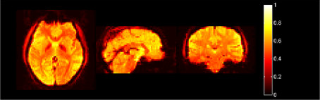
(a)

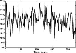
(b)

Figure 1: Example of fMRI data set for a single subject from the 1000 connectome Beijing data. The top image (a) shows a three-dimensional view of the temporally averaged brain data and is formally equivalent to the mean function for these data. The bottom image (b) shows the time series for the central voxel of the image. The analysis considers all the time series of all the voxels together (as a single functional time series).

volume present. In this paper, we will consider the spatial data as a function, and the time series to be repeated (and correlated) observations of that function. This implies that the spatial covariance function will be six-dimensional, and it is this covariance that is intrinsically of interest in resting state fMRI studies (as connectivity maps are simply approximations to this covariance). While it might be possible in individual cases to use a supercomputer to handle matrices of this order [see Long et al. (2011), e.g.], in most cases where there are large numbers of subjects to process, an approximation, or, equivalently, dimension reduction, will be needed, and this will now be the focus of the next section.

3 Projections for functional data

In functional neuroimaging, two main analysis options are usually considered: mass univariate analysis or projection subspace analysis. Examples of the second include analyses such as those using eigenimages [Friston et al. (1993)] and independent component analysis (ICA) [see Beckmann and Smith (2005), e.g.]. In this paper, a projection subspace approach will be taken.

In this section we detail some projections that can be used for functional observations $X_{t}(u),u\in\mathcal{U}$, $t=1,\ldots,n$, where $\mathcal{U}$ is some compact set. In fMRI, this corresponds to $u$ being the voxel location in the brain (or a continuous analogue of a voxel), while $t$ is the scan number from the total $n$ scans taken. Thus, the complete brain itself is treated as a single function and this function is observed $n$ times. Of course, due to slice timing events and voxel discretizations, this will be an approximation, but one which naturally encodes the brain as a single observed unit. However, should a high-dimensional multivariate approach be preferred, the results in this paper will equally apply. In addition, we will assume that each fMRI observation is made up of a common mean function $\mu(u)$, that is, $X_{t}(u)=\mu(u)+Y_{t}(u)$ where $Y_{t}(u)$ are deviations from the mean [with assumed mathematical properties $\{Y_{t}(u)\dvtx 1\leq t\leq n\}$ are elements of $L^{2}(\mathcal{U})$, $\mathrm{E}Y_{t}(u)=0$ and form a stationary time series].

Below, we will define an orthonormal system $\{\widehat{v}_{j}(\cdot),j=1,\ldots,d\}$ for the projection components. Associated with each system is the score, which is determined by the inner product of the data with the component, $\widehat{\eta}_{t,l}:=\langle X_{t},\widehat{v}_{l}\rangle=\int_{\mathcal{U}}X_{t}(u)\widehat{v}_{l}(u)\,du$.

The orthonormal system could be either chosen in advance, as in, for example, wavelet based methods for functional data, or derived from the data, as in functional principal components. In particular, if a region based analysis in fMRI of connectivity was of interest, then the regions of interest can be expressed as a projection of the original data. In such a situation, whether this regional data is stationary or not is the key question, and thus the tests of the next section should be applied using this projection. Otherwise, if the stationarity of the complete data is of interest rather than that of a specific projection, then a projection should be chosen that also contains the nonstationarities. Possible methods for choosing bases include principal component analysis (PCA) or ICA. ICA is very popular in resting state analyses [Beckmann et al. (2005)], but PCA is often a preprocessing step in the ICA analysis and additionally is very much linked to the analysis of covariances, which plays a prime role in connectivity analysis, and therefore we shall concentrate on PCA here. It will also be shown in Section 5.3.2 that estimating the projections using PCA can have good power for detecting nonstationarites. As estimation of PCA components is more complex than nonestimated bases, we will concentrate on this case (with analogous results for the testing and estimation procedures of Section 4 following in the nonestimated basis function case).

3.1 Principal components

Classical dimension reduction techniques are often based on the first $d$ principal components, which choose a subspace explaining most variance for any subspace of an equivalent dimension. The notation below is in terms of integrals, which is simply the function based analogue of traditional multivariate vector based PCA. To elaborate, consider the (spatial) covariance kernel of $Y_{t}(\cdot)$ given by

$$c(u,s)=\mathrm{E}\bigl{(}Y_{t}(u)Y_{t}(s)\bigr{)}$$ (1)

and define the covariance operator $C\dvtx\mathcal{L}^{2}(\mathcal{U})\to\mathcal{L}^{2}(\mathcal{U})$ by $Cz=\int_{\mathcal{U}}c(\cdot,s)z(s)\,ds$.

Let $\{\lambda_{k}\}$ be the nonnegative decreasing sequence of eigenvalues of the covariance operator and $\{v_{k}(\cdot)\dvtx k\geq 1\}$ a given set of corresponding orthonormal eigenfunctions, that is,

$$\int c(u,s)v_{l}(s)\,ds=\lambda_{l}v_{l}(u),\qquad l=1,2,\ldots,u\in\mathcal{U}.$$ (2)

$Y_{t}(\cdot)$ can be expressed in terms of the eigenfunctions

$$Y_{t}(u)=\sum_{l=1}^{\infty}\eta_{t,l}v_{l}(u),$$ (3)

where

$$\eta_{t,l}=\int Y_{t}(u)v_{l}(u)\,du,\qquad t=1,\ldots,n,l=1,2,\ldots,$$ (4)

are uncorrelated with mean $0$ and variance $\lambda_{l}$. More details can, for example, be found in either Bosq (2000) or Horváth and Kokoszka (2012).

A natural estimator in a general nonparametric setting is the empirical version of the covariance function (analogously to standard PCA)

$$\widehat{c}_{n}(u,s)=\frac{1}{n}\sum_{t=1}^{n}\bigl{(}X_{t}(u)-\bar{X}_{n}(u)\bigr{)}\bigl{(}X_{t}(s)-\bar{X}_{n}(s)\bigr{)},$$ (5)

where $\bar{X}_{n}(u)=\frac{1}{n}\sum_{t=1}^{n}X_{t}(u)$.

Usually one converts the continuous functional eigenanalysis problem to an approximately equivalent matrix eigenanalysis task. The simplest solution is a discretization of the observed function on a fine grid. Many data sets in applications are already obtained in this way, as in the example of fMRI data used in this paper. For a discussion of this as well as more advanced options, we refer to Ramsay and Silverman (2005). In such examples of very high-dimensional data, a PCA based on the empirical covariance matrix is computationally infeasible due to the even higher-dimensionality of the covariance matrix. The following computational trick can be applied but also shows the limitations of the approach, as the number of nonzero eigenvalues of the estimated covariance matrix is limited by the sample size, with the associated problems for small sample sizes.

Assume that after discretization the data are given by $X_{t}:=(X_{t}(1),\ldots,\allowbreak X_{t}(M))^{T}$, $t=1,\ldots,n$. In fMRI, $M$ here would be the total number of voxels. The eigenanalysis problem corresponding to the estimated covariance kernel in (5) is to find the eigenvalues of the $M\times M$-matrix $ZZ^{T}$, where $Z=(X_{1}-\bar{X}_{n},\ldots,X_{n}-\bar{X}_{n})$ is a $M\times n$-matrix. One can check that $ZZ^{T}$ has $\operatorname{rank}(Z)\leq\min(M,n)$ nonzero eigenvalues which coincide with the $\operatorname{rank}(Z)\leq\min(M,n)$ nonzero eigenvalues of the $n\times n$-matrix $Z^{T}Z$. This is equivalent in fMRI to saying that there is a relation between the covariance matrix of space (a huge $M\times M$ matrix) and that of the time dimension ($n\times n$ matrix). Furthermore, the eigenvectors $v_{k}$ of $ZZ^{T}$ can be obtained from the eigenvectors $v^{\prime}_{k}$ of $Z^{T}Z$ by

$$v_{k}=\frac{Zv^{\prime}_{k}}{\|Zv^{\prime}_{k}\|},\qquad k=1,\ldots,\operatorname{rank}(Z).$$

For more details we refer to Härdle and Simar (2007), Chapter 8.4. This indicates that temporal eigenvectors and spatial eigenvectors are intrinsically linked due to the way the data is discretely collected with no physical meaning whatsoever. Without presmoothing of the observed data, it can easily happen that $M\gg n$ (as is the case of fMRI where the number of voxels usually far exceeds the number of time points). This implies that a maximum of $n$ different components can be found. Consequently, even though there are hundreds of thousands of voxels recorded, only a few hundred components are actually identifiable, if the analysis proceeds in this generic way. In the case where $M\gg n$, it is computationally much faster to calculate the eigenvectors of $Z^{T}Z$ and then use the above transformation to obtain the eigenvectors of $ZZ^{T}$. This computational idea has been used for magnetic resonance imaging data (anatomical imaging rather than fMRI) in an i.i.d. setting in Zipunnikov et al. (2011).

3.2 Separable covariance structures

The above discussion suggests that in many settings a loss of precision is unavoidable when the nonparametric covariance estimator (5) is used with such high-dimensional data. Therefore, in this section we assume a separable data structure which reduces the number of unknown parameters and can significantly improve computational speed as well as accuracy, at least in situations where the data structure is correctly specified. The use of separable functions for brain imaging is well known, either for smoothing [Worsley et al. (2002)] or signal processing using techniques such as separable wavelets [Ruttimann et al. (1998)], both of which indirectly imply separable covariances.

As well as having been previously suggested for multivariate covariances for images [see Dryden et al. (2009) for an example and related references], separable covariance structures have obtained significant attention in the context of spatio-temporal statistics, where they have been used to separate the purely temporal covariance from the purely spatial covariance [see Fuentes (2006) and Mitchell, Genton and Gumpertz (2005)]. While in our setup a temporal dependency is also present, we use the separability approach only on the multidimensional spatial structure mainly for computational reasons to get a better and more stable approximation of the eigenfunctions in situations where the temporal sample is only moderately sized and the spatial structure is very high dimensional.

For clarity of explanation, two-dimensional data sets will be discussed here, although identical arguments apply for any finite number of dimensions. Indeed, the fMRI data set we consider is three dimensional so that a three-dimensional version of the procedure below is used.

To this end, consider the set $\mathcal{U}_{1}\times\mathcal{U}_{2}$, which is a product of two compact sets. Heuristically, these can be thought of as the two directions in a planar image. Let $X_{t}(u_{1},u_{2}),u_{1}\in\mathcal{U}_{1},u_{2}\in\mathcal{U}_{2}$, $t=1,\ldots,n$, and under $H_{0}$,

$$X_{t}(u_{1},u_{2})=Y_{t}(u_{1},u_{2})+\mu(u_{1},u_{2}),$$ (6)

where the mean function $\mu(\cdot,\cdot)$ as well as the functional stationary time series $\{Y_{t}(\cdot,\cdot)\dvtx 1\leq t\leq n\}$ are elements of $L^{2}(\mathcal{U}_{1}\times\mathcal{U}_{2})$, $\mathrm{E}Y_{t}(u_{1},u_{2})=0$.

The restricted covariance kernel of $Y_{1}(\cdot,\cdot)$ is assumed to fulfill

$$c\bigl{(}(u_{1},u_{2}),(s_{1},s_{2})\bigr{)}=c_{1}(u_{1},s_{1})c_{2}(u_{2},s_{2}),$$ (7)

where $c_{1}(u_{1},s_{1})$ is an element of $L^{2}(\mathcal{U}_{1}\times\mathcal{U}_{1})$ and $c_{2}(u_{2},s_{2})$ an element of $L^{2}(\mathcal{U}_{2}\times\mathcal{U}_{2})$, with the full covariance function being an element of $L^{2}((\mathcal{U}_{1}\times\mathcal{U}_{2})\times(\mathcal{U}_{1}\times\mathcal{U}_{2}))$. An important example of random data having such a separable structure is the following: assume $Y$ has mean 0 and covariance kernel $c_{Y}(u_{1},s_{1})$ independent of $X$, which has mean 0 and covariance kernel $c_{X}(u_{2},s_{2})$, then $Z(u_{1},u_{2})=Y(u_{1})X(u_{2})$ has covariance kernel $c_{Y}(u_{1},s_{1})c_{X}(u_{2},s_{2})$. In this example the data set itself is separable, from which the separability of the covariance as well as sample covariance kernel follows.

The factors $c_{1}$ and $c_{2}$ can only be obtained up to a multiplicative constant as

$$c\bigl{(}(u_{1},u_{2}),(s_{1},s_{2})\bigr{)}=\bigl{(}\alpha c_{1}(u_{1},s_{1})\bigr{)}\biggl{(}\frac{1}{\alpha}c_{2}(u_{2},s_{2})\biggr{)},\qquad\alpha\neq 0,$$

but this does not cause a problem for the change-point procedures, as will be seen below.

As in the nonparametric case, one uses a discretized version of the covariance matrix for computations, so that this approach significantly reduces the computational complexity. For instance, if the observations consist of 100 data points in each direction (as is approximately the case in one slice of an fMRI image), the covariance “matrix” $c$ is a $10\mbox{,}000\times 10\mbox{,}000$ matrix, while $c_{1}$ and $c_{2}$ are of dimension $100\times 100$ each. The covariance matrix of a two-dimensional data set $Z$ can, for example, be obtained as the covariance matrix of $\widetilde{Z}=\operatorname{vec}(Z)$, where $\operatorname{vec}$ is the operation that turns matrices into vectors by “stacking” the columns. Under the above separability assumption, the covariance matrix of $\widetilde{Z}$ corresponds to $c=c_{1}\otimes c_{2}$, where $\otimes$ is the Kronecker product. Obviously the gains from this procedure will be even more in a 3-D fMRI image, where the corresponding full covariance will be of the order $10^{5}\times 10^{5}$.

Furthermore, several approaches to estimate $c_{1}$ and $c_{2}$ from the data in a multivariate setting have been discussed in the literature. Van Loan and Pitsianis (1993) propose an algorithm which approximates a possibly nonseparable covariance matrix by the closest (in the Frobenius norm) Kronecker product which has been shown to be useful in spatio-temporal covariance matrix approximation [Genton (2007)]. While this is a very appealing approach, especially in view of misspecification, it is computationally not feasible in a high-dimensional context, as it involves the calculation of singular vectors, which is computationally very expensive. Dutilleul (1999) proposes an MLE algorithm to estimate the factors, but again for high-dimensional data it is computationally too slow. However, their approach is related in the sense that they propose to start their algorithm with our estimator below. This amounts to our estimator being asymptotically unbiased but not efficient (although computationally feasible, which is one of our main requirements). Extended and related algorithms have also been proposed for the estimation of separable covariance functions in a signal processing context [Werner, Jansson and Stoica (2008)] but are again designed for the use in small-dimensional problems.

The covariance kernels

$$c_{1}(u_{1},s_{1})=\int_{\mathcal{U}_{2}}c\bigl{(}(u_{1},z),(s_{1},z)\bigr{)}\,dz$$ (8)

and, equivalently, $c_{2}(u_{2},s_{2})$ also need to be estimated from the discretely observed data. Here we adopt an approach based on the empirical covariance,

$$\widehat{c}_{1}(u_{1},s_{1})=\int_{\mathcal{U}_{2}}\widehat{c}\bigl{(}(u_{1},z),(s_{1},z)\bigr{)}\,dz,$$ (9)

where $\widehat{c}((u_{1},u_{2}),(s_{1},s_{2}))$ is the multidimensional analogue of (5). For discretely sampled data (as in fMRI), the integral is approximated by the following sum:

$$\frac{1}{n}\sum_{t=1}^{n}\frac{1}{|\mathcal{U}_{2}|}\sum_{z\in\mathcal{U}_{2}}\bigl{(}X_{t}(u_{1},z)-\bar{X}_{n}(u_{1},z)\bigr{)}\bigl{(}X_{t}(s_{1},z)-\bar{X}_{n}(s_{1},z)\bigr{)},$$ (10)

where $\mathcal{U}_{2}$ in (10) is the set of discrete observations of the function in the second direction (and where in the 3-D fMRI data, $|\mathcal{U}_{1}|=64$, $|\mathcal{U}_{2}|=64$, and $|\mathcal{U}_{3}|=33$, yielding a combined $|\mathcal{U}|\approx 135\mbox{,}000$). This approximation amounts to estimating covariances in one direction while keeping the other directions fixed, and then averaging over the results. A completely analogous definition for $\widehat{c}_{2}(u_{2},s_{2})$ can be used. The individual functions are only identified up to a multiplicative constant, but the eigenfunctions are identifiable up to their sign. For details we refer to Section 5.3.1, while Table 1 gives an outline of the overall procedure. This approach not only inherently provides more data to estimate each set of directional components compared with the standard approach, but also allows more than the maximum $n$ components identifiable in the generic nonseparable procedure to be estimated as nonzero.

Table 1: Steps to compute separable eigenfunctions

1	For each of $k$ dimensions calculate the univariate directional covariance function with replicates across both time and the other dimensions. Note that the unidentifiable constants do not matter so can be set to any arbitrary value, for example, in two dimensions, the first directional covariance function is $$c_{1}(u_{1},s_{1})=\frac{1}{n}\sum_{t=1}^{n}\frac{1}{|\mathcal{U}_{2}|}\sum_{z\in\mathcal{U}_{2}}\bigl{(}X_{t}(u_{1},z)-\bar{X}_{n}(u_{1},z)\bigr{)}\bigl{(}X_{t}(s_{1},z)-\bar{X}_{n}(s_{1},z)\bigr{)}.$$
2	For each directional covariance $i$, $i=1,\ldots,k$, obtain eigenfunctions $\widehat{v}_{i,j}$ and $\widehat{\lambda}_{i,j}$.
3	Order the $\widehat{\lambda}_{i,j}$ and for each $i$, select select the top $d_{i}$, for example, $d_{i}=\sqrt[k]{d}$, eigenfunctions.
4	Take the tensor product of the selected eigenfunctions to obtain the eigenbasis, $\displaystyle\{\widehat{v}_{1,j_{1}}\otimes\cdots\otimes\widehat{v}_{1,j_{k}},j_{l}=1,\ldots,d_{l},l=1,\ldots,k\}.$

In real data, separability can be a somewhat difficult assumption to verify empirically. However, even if separability is not a valid assumption, the above procedure still provides a completely valid projection. The estimated basis functions will just no longer coincide with the eigenfunctions. However, none of the subsequent methodology for the change-point model which will be developed in Section 4 is limited to principal components, so the procedure remains useful even in the case of nonseparable data.

3.3 Separable principal component analysis of the connectome data

In Figure 2, a resting state fMRI data set is shown after a separable dimension reduction to 64 ($=4\times 4\times 4$) dimensions was conducted, using separable projections and finding the covariance functions using (9) from the previous section. Recall that the original dimensions are

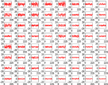
Figure 2: Subject 69518: a 64 component functional PCA decomposition of the brain from this subject (the number of observed spatial locations is well in excess of 100,000, and thus this represents a massive dimension reduction). As will be seen later, when testing for change-points, there was no evidence of an epidemic change for this subject. This is noticeable in the figure, in that no individual graph contains sustained deviations in one direction from the mean above those which might be expected from examining 64 realizations of stationarity.

$64\times 64\times 33$ and therefore more than 2000 times as high. Indeed, the traditional way of choosing the number of components uses some threshold for the amount of variance to be explained. For the above subject (and similarly for the other subjects) 64 components explain less than 1% of the variation, which would seem to be of little use in a dimension reduction context. However, by performing a careful statistical analysis of the relationship between the type of change-points to be detected and the choice of the projection, it will be seen that in many instances, even such a small number of components will be enough.

4 Change-point testing and estimation

4.1 Models for fMRI change-points

Activations in brain imaging are typically modeled as changes from baseline for a short period followed by a return to baseline [see, e.g., Worsley et al. (2002)] showing that level shifts or change-point models describe well the kind of deviation from stationarity that can be expected. However, in resting state scans, it is not known when or even if any changes occur across time and, thus, change-point methods become more applicable than traditional experimental regression response type models. In addition, epidemic changes as the simplest model for multiple changes are a good first approximation to the deviation from stationarity that can be expected.

The epidemic model is given by

$$X_{t}(u)=Y_{t}(u)+\mu(u)+\Delta(u)1_{\{\vartheta_{1}n<t\leq\vartheta_{2}n\}},$$ (11)

where $\mu(u)$ is the underlying activation pattern for a particular subject, and as such does not need to be registered to a standard space for the model to be evaluated. $Y_{t}(u)$ is the stationary statistical deviation from this underlying pattern (it is the stationary covariance structure of these deviations which are of most interest in connectivity studies). Here, $\Delta(u)$ is the simplified deviation from stationarity (a mean change that persists for a given amount of the scan, for a fraction $\vartheta_{1}$ to $\vartheta_{2}$ of the scan, as given by the $1$ indicator function). Similarly, in a separable situation, the definition of the model is completely analogous, for example, in two dimensions,

$$X_{t}(u_{1},u_{2})=Y_{t}(u_{1},u_{2})+\mu(u_{1},u_{2})+\Delta(u_{1},u_{2})1_{\{\vartheta_{1}n<t\leq\vartheta_{2}n\}}.$$

The epidemic model compares to the AMOC-model, which is given by

$$X_{t}(u)=Y_{t}(u)+\mu(u)+\Delta(u)1_{\{\vartheta n<t\leq n\}},$$ (12)

where once the change has occurred it persists for the rest of the scanning session. We believe that in fMRI studies, epidemic models are more realistic, but analogous versions of all the results of the paper are equally valid for AMOC models.

We are interested in testing the null hypothesis of no change in the mean

$$H_{0}\dvtx\mathrm{E}X_{t}(\cdot)=\mu(\cdot),\qquad t=1,\ldots,n,$$

versus the epidemic change alternative

$$H_{1}\mbox{:\quad}\mathrm{E}X_{t}(\cdot) = \mu(\cdot),\qquad t=1,\ldots,\lfloor\vartheta_{1}n\rfloor,\lfloor\vartheta_{2}n\rfloor+1,\ldots,n,\qquad\mbox{but}$$

$$\mathrm{E}X_{t}(\cdot) = \mu(\cdot)+\Delta(\cdot)\neq\mu(\cdot),$$ (13)

$$\eqntext{t=\lfloor\vartheta_{1}n\rfloor+1,\ldots,\lfloor\vartheta_{2}n\rfloor,\qquad 0<\vartheta_{1}<\vartheta_{2}<1.}$$

The null hypothesis corresponds to the cases where $\vartheta_{1}=\vartheta_{2}=1$.

The setting for independent (functional) observations with AMOC was investigated by Berkes et al. (2009) as well as Aue et al. (2009) and for specific weak dependent processes by Hörmann and Kokoszka (2010). We will also allow for dependency (in time) of the functional observations and focus on the model with an epidemic change, where after a certain time the mean changes back. For this model some theoretical results relating to the detection and estimation of changes are given in Aston and Kirch (2012b). The required mathematical setup for the problem is given in Section S.1 of the supplementary material [Aston and Kirch (2012a)].

4.2 Projections under the null and alternative hypotheses

In classical statistical situations, dimension reduction using principal components is useful because it maximizes the variance explained by the projection. In the change-point situation, principal components are also especially suitable but for completely different reasons. Heuristically speaking, standard variance estimators (such as the sample variance) increase in the presence of level shifts. Similarly, the variance estimate for linear combinations of components in the multivariate situation based on empirical covariances will increase if a change is present in the linear combination. Thus, under the alternative, the principal components of the estimated covariance matrix will likely contain a change [indicating that assumption (21), given later, is fulfilled].

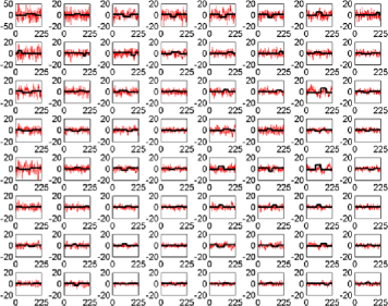
Figure 3: Subject 01018: dimension reduction along with possible epidemic changes indicated (thick black line). Using the tests described, this subject was found to have deviations from stationarity, $p<0.001$, even when corrected for multiple comparisons using FDR. This is most clearly seen in that several of the individual graphs have large possible sustained deviations in one direction from the mean.

The subject in Figure 3 seems to exhibit strong deviations from stationarity—in fact, the $p$-value associated with this subject is below $0.001$ based on the bootstrap test given in Section 7. It should be stressed that the change detection is a global hypothesis test combined over all components considered. In this way, while taking more components will help increase the chance that the change is present in one, it will come at the cost of the size of the change needed in finite samples for an omnibus test of this type. However, the subject shown in the figure did cause a rejection of the null hypothesis of no change both in the 64 and 125 subspace size omnibus tests. While the pictures in Figure 3 indicate that an epidemic change is indeed a good first approximation for the nonstationarities occurring for this particular subject, more deviation (maybe more change-points) does seem to be present. In Figure 4, a second subject is shown with a much smaller deviation from stationarity (most of the components seem to have little to no possible mean change present), which is significant but does not survive the false discovery rate (FDR) correction (see Section 4.3).

4.3 Test statistic and estimator of change-point locations

For a $d$-dimensional subspace projection, Aston and Kirch (2012b) propose to use the following standard change-point statistics for an epidemic change on the projected data $\widehat{\bolds{\eta}}_{t}=(\widehat{\eta}_{t,1},\ldots,\widehat{\eta}_{t,d})^{T}$:

$$T_{n}^{(A)} = \frac{1}{n^{3}}\sum_{1\leq k_{1}<k_{2}\leq n}\mathbf{S}_{n}({k_{1}}/{n},{k_{2}}/{n})^{T}\widehat{\bolds{\Sigma}}{}^{-1}\mathbf{S}_{n}({k_{1}}/{n},{k_{2}}/{n}),$$

$$T_{n}^{(B)} = \max_{1\leq k_{1}<k_{2}\leq n}\frac{1}{n}\mathbf{S}_{n}({k_{1}}/{n},{k_{2}}/{n})^{T}\widehat{\bolds{\Sigma}}{}^{-1}\mathbf{S}_{n}({k_{1}}/{n},{k_{2}}/{n}),$$

where $\widehat{\bolds{\Sigma}}$ is a consistent estimator for the long-run covariance matrix [as defined in (19)] and

$$\mathbf{S}_{n}(x,y)=\sum_{nx<j\leq ny}\Biggl{(}\widehat{\bolds{\eta}}_{j}-\frac{1}{n}\sum_{t=1}^{n}\widehat{\bolds{\eta}}_{t}\Biggr{)}.$$

For the small sample performance of the test the choice of estimator $\widehat{\bolds{\Sigma}}$ is crucial, which is why this issue is discussed in detail in Section 6.1.

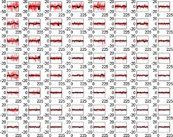
Figure 4: Subject 48501: dimension reduction along with possible epidemic changes indicated (thick black line). Using the tests described, this subject was found to have deviations from stationarity, $p<0.05$, but not evidence of deviations when using FDR multiple comparisons correction. In this case some individual graphs seem to show more evidence of mean change than in Figure 2 but less coherence in terms of time than some in Figure 3.

The main aim of the test statistics above is to determine regions where the mean differs significantly from the overall mean of the complete time series. If these differences are larger than a threshold, then a change-point is deemed to have occurred. The limit distributions of the statistics will be found in Section 5.2. If the value is above the threshold, then in the same way as with many CUSUM type change-point tests, good estimators are usually obtained for the change-point locations by taking the points where the statistics achieve their maximum. Thus, as an estimator for the change-points, we propose

$$(\widehat{\vartheta}_{1},\widehat{\vartheta}_{2})=\arg\max\bigl{(}\mathbf{S}_{n}^{T}(x,y)\widehat{\bolds{\Sigma}}{}^{-1}_{n}\mathbf{S}_{n}(x,y)\dvtx 0\leq x<y\leq 1\bigr{)},$$ (15)

where $\mathbf{S}_{n}(x,y)$ is as above and $(x_{1},y_{1})=\arg\max(Z(x,y)\dvtx 0\leq x<y\leq 1)$ iff $x_{1}=\min(0\leq x<1\dvtx Z(x,y)=\max_{0\leq s<t\leq 1}Z(s,t)$ for some $y)$ and $y_{1}=\max(y>x_{1}\dvtx Z(x_{1},y)=\max_{0\leq s<t\leq 1}Z(s,t))$.

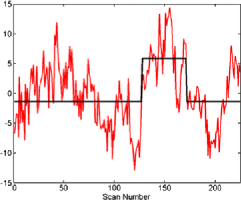
(a)

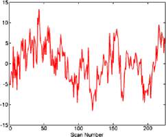
(b)

Figure 5: Subject 01018: for this subject there is evidence of deviations from stationarity, $p<0.001$. This figure shows a candidate component 23 time series (a) before and (b) after correction using the estimated change-point location.

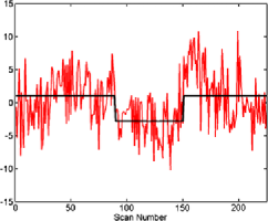
(a)

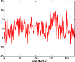
(b)

Figure 6: Subject 48501: for this subject there is evidence of deviations from stationarity, $p<0.05$, but it is no longer rejected when using FDR multiple comparisons correction. This figure shows a candidate component 7 time series (a) before and (b) after correction using the estimated change-point location.

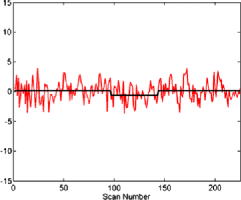
(a)

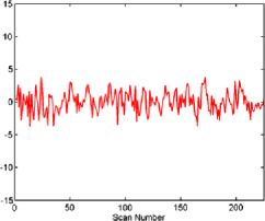
(b)

Figure 7: Subject 48501: as mentioned above, for this subject there is evidence of weak deviations from stationarity, $p<0.05$, but not rejected when using FDR multiple comparisons correction. This figure shows one of the components from the subject that has little evidence of any kind of nonstationarity present. While the black line results from the estimator from the maximum of the change-point statistic, it is not a viable candidate series to contain nonstationarities. (a) Component 56 time series; (b) component 56: epidemic change removed.

Figures 5–7 show three component time series selected for their different properties. The component in Figure 5 can be seen to be a candidate series for a change to have occurred with the resulting change corrected series visually appearing much more stationary (although it is likely there are other nonstationarities present as well). This series, from subject 01018 in the connectome data set, was found to have evidence of nonstationarities when the sample version of the statistic (given in Section 6.2) was tested on both a 64 and 125 component projection.

When testing subject 48501 from the connectome data, from whom the components can be seen in Figure 4, an epidemic change seems to be quite a good model for several components, but only a small part of the time series deviates from stationarity. For example, component 7 in Figure 6 shows a less pronounced but still plausible epidemic change compared with component 23 of subject 01018 in Figure 5. However, as can be seen in another component (Figure 7) from subject 48501, some of the components seem to be stationary without any change present.

Given that nearly 200 subjects were tested, a multiple comparison correction was implemented using the independent FDR method by Benjamini and Hochberg (1995). The use of an independent FDR is based on the fact that the comparisons are being taken across subjects who can be assumed to be independent of each other. Subject 01018 (Figure 3) survived the FDR correction and evidence was still found of nonstationarities being present. Subject 48501, whose projections are seen in Figure 4, also rejected the null hypothesis but only at about a 3% level, hence not surviving the FDR correction.

Finally, in Figure 2 the subject shown has components which do not indicate level shifts and, in fact, the null hypothesis is not rejected for this subject, either with or without FDR correction.

4.4 Questions associated with the application of the above procedures to fMRI data

While the discussion above provides a procedure for obtaining test statistics for functional data in very high-dimensional settings such as fMRI, it naturally leads to a number of questions, which the remainder of the paper seeks to address. These questions and the sections where they are addressed are as follows: [(5)]

Could the projected data exhibit a different type of alternative than the one we are looking for in the full functional time series. In particular, if there is an epidemic change in the fMRI data, will there still be an epidemic change in any nonstationary component derived from the projection? (See Section 5.1.)

Is there a limit distribution available for these test statistics under the null hypothesis such that critical values can be obtained so that deviations from stationarity can be determined for fMRI? What happens to the statistics under the alternative hypothesis, that is, when there are nonstationary portions in the brain activity? (See Section 5.2.)

How is the power of the test (possibility of detecting changes) related to the projection that is taken? This is critical if only a small number of components can feasibly be taken, as in the case of fMRI, where computational considerations will dominate. (See Section 5.3.2.)

Can this all be done when there are only relatively small samples of functional data available (an fMRI time series is typically only a few hundred time points with hundreds of thousands of spatial locations)? (See Section 6.2.)

As most fMRI studies have multiple subjects, can information about change-points be generalized to the population? (See Section 8.)

5 Some statistical properties of the test statistics

5.1 Projections under stationarity and level shifts

The entire brain covariance structure in an fMRI data set, as represented by the covariance kernel $c(u,s)$, is not known and needs to be estimated. However, even if $c(u,s)$ were known, using estimators would often be preferable due to the nice property that the estimated covariance can be influenced by the change in such a way that the change becomes detectable in a lower-dimensional projection (cf. Corollary 5.1). Thus, even if we knew how the brain varied in a stationary condition, it would be preferable to use estimators unless we knew exactly in which lower-dimensional projections the changes will have occurred (or if, as in a region based analysis, we are only interested in the stationarity of the projection rather than the full data). Thus, we need to examine the behavior of projections under the alternative.

Under an epidemic change alternative ($t=1,\ldots,n,l=1,\ldots,d$),

$$\quad\widehat{\eta}_{t,l}:=\langle X_{t},\widehat{v}_{l}\rangle=\int X_{t}(u)\widehat{v}_{l}(u)\,du=\langle Y_{t},\widehat{v}_{l}\rangle+1_{\{\vartheta_{1}n<t\leq\vartheta_{2}n\}}\langle\bolds{\Delta},\widehat{v}_{l}\rangle.$$ (16)

In particular, $\widehat{\bolds{\eta}}_{t}=(\widehat{\eta}_{t,1},\ldots,\widehat{\eta}_{t,d})^{T}$ is a $d$-dimensional time series exhibiting the same type of level shifts, that is, an epidemic change in this case, as the functional sequence $\{X_{t}(\cdot)\dvtx 1\leq t\leq n\}$ if the change is not orthogonal to the subspace spanned by $\widehat{v}_{1}(\cdot),\ldots,\widehat{v}_{d}(\cdot)$.

From (16) it is obvious that the choice of estimation procedure for basis functions has a substantial influence under the alternative on the size of $\langle\bolds{\Delta},\widehat{v}_{l}\rangle$, hence the visibility and detectability of the change. In other words, the behavior of this estimation procedure under alternatives is crucial for the power of the test. As a contrast, the estimation procedure has only a very mild influence on the behavior under the null hypothesis.

Under the null hypothesis, we require the estimated orthonormal system (ON-system) $\{\widehat{v}_{l}(\cdot),l=1,\ldots,d\}$ (assuming $d$ distinct eigenvalues) to stabilize in the following sense for technical reasons:

$$\int\bigl{(}\widehat{v}_{l}(u)-s_{l}v_{l}(u)\bigr{)}^{2}\,du=O_{P}\bigl{(}n^{-1}\bigr{)},$$ (17)

where $s_{l}=\operatorname{sgn}(\int v_{l}(u)\widehat{v}_{l}(u)\,du)$ and $\{v_{l}(\cdot),l=1,\ldots,d\}$ is some orthonormal system. In particular, $\{\widehat{v}_{l}(\cdot),l=1,\ldots,d\}$ is a consistent estimator of $\{v_{l}(\cdot),l=1,\ldots,d\}$ up to the sign. In addition, if the basis is fixed, as in a wavelet based or region based analysis, this proposition is fulfilled by definition.

It cannot, in general, be expected that the same limit of the estimated eigenfunctions will occur under both the null and alternative hypothesis. However, having different limits can actually be favorable when detecting changes, as will be seen in Corollary 5.1. Thus, under the alternative we require that

$$\int\bigl{(}\widehat{v}_{l}(u)-s_{l}w_{l}(u)\bigr{)}^{2}\,du=o_{P}(1),$$ (18)

where $\{w_{l}(\cdot),l=1,\ldots,d\}$ is an orthonormal system, $\{\widehat{v}_{l}(\cdot),l=1,\ldots,d\}$ the same estimators as before and $s_{l}=\operatorname{sgn}(\int w_{l}(u)\widehat{v}_{l}(u)\,du)$, that is, the estimators converge to some contaminated ON-system. Note that $w_{l}$ usually depends on the alternative. Indeed, most statistical procedures, including PCA, will still have stable behavior even in the presence of nonstationarities.

None of the above properties require the basis to be the principal component basis. However, as will be seen in Section 5.3, PCA does indeed fulfil the properties (17) and (18) given above.

5.2 Asymptotic evaluation

Under (17) and the time series assumptions given in Section S.1.2, and where in (4.3) the long run covariance is defined to be

$$\bolds{\Sigma}=\sum_{k\in\mathbb{Z}}\Gamma(k),\qquad\Gamma(h)=\mathrm{E}\bolds{\eta}_{t}\bolds{\eta}_{t+h}^{T}$$ (19)

for $h\geq 0$, and $\Gamma(h)=\Gamma(-h)^{T}$ for $h<0$, Aston and Kirch (2012b) prove the following asymptotics under $H_{0}$:

$$T_{n}^{(A)} \stackrel{{\scriptstyle\mathcal{L}}}{{\longrightarrow}} \sum_{1\leq l\leq d}\int\!\!\int_{0\leq x<y\leq 1}\bigl{(}B_{l}(x)-B_{l}(y)\bigr{)}^{2}\,dx\,dy,$$

$$T_{n}^{(B)} \stackrel{{\scriptstyle\mathcal{L}}}{{\longrightarrow}} \sup_{0\leq x<y\leq 1}\sum_{1\leq l\leq d}\bigl{(}B_{l}(x)-B_{l}(y)\bigr{)}^{2},$$

where $B_{l}(\cdot)$, $l=1,\ldots,d$, are independent standard Brownian bridges.

In order to obtain asymptotic power one for the above tests, the estimation procedure additionally needs to stabilize under alternatives, as in (18). The change can only be detected if it is not orthogonal to the contaminated ON-system, that is, for some $k=1,\ldots,d$ it holds

$$\int\Delta(u)w_{k}(u)\,du\neq 0.$$ (21)

Then, Aston and Kirch (2012b) show that under the epidemic change alternative

$$T_{n}^{(A)}\stackrel{{\scriptstyle P}}{{\longrightarrow}}\infty,\qquad T_{n}^{(B)}\stackrel{{\scriptstyle P}}{{\longrightarrow}}\infty,$$

if $\widehat{\bolds{\Sigma}}\stackrel{{\scriptstyle P}}{{\longrightarrow}}\bolds{\Sigma}_{A}$ for some symmetric positive-definite matrix $\bolds{\Sigma}_{A}$. This shows that the power of the test is mostly affected by the estimation procedure to obtain the orthonormal basis for the projection.

Aston and Kirch (2012b) prove that the change-point estimator related to the above test as given in (15) is consistent under the assumptions in Section S.1.1 and even get the following rate given slightly stronger assumptions:

$$(\widehat{\vartheta}_{1},\widehat{\vartheta}_{2})-(\vartheta_{1},\vartheta_{2})=O_{P}\bigl{(}n^{-1/2}\bigr{)}.$$ (22)

5.3 Specifics for principal component analysis

When using PCA, the basis is defined from the data via the empirical covariance function. Thus, the properties of the empirical estimator of the covariance are important. In order to get (17), we require that the estimated covariance kernel $\widehat{c}_{n}(u,s)$ is a consistent estimator for the covariance kernel $c(u,s)$ of $\{Y_{1}(\cdot)\}$ with convergence rate $\sqrt{n}$ under $H_{0}$, that is,

$$\int\!\!\int\bigl{(}\widehat{c}_{n}(u,s)-c(u,s)\bigr{)}^{2}\,du\,ds=O_{P}\bigl{(}n^{-1}\bigr{)}.$$ (23)

Aston and Kirch (2012b) show that strong mixing and other weak dependent sequences fulfill this assumption. This condition implies that (17) holds for standard PCA, with $v_{l}(u)$ being the associated principal components [Aston and Kirch (2012b)]. The equivalent result for separable PCA will be discussed in the next section.

Under the alternative $H_{1}$, we assume that there exists a covariance kernel $k(u,s)$, such that

$$\int\!\!\int\bigl{(}\widehat{c}_{n}(u,s)-k(u,s)\bigr{)}^{2}\,du\,ds\stackrel{{\scriptstyle P}}{{\longrightarrow}}0,$$ (24)

which similarly implies that (18) holds, with $w_{l}(u)$ being the associated principal components [Aston and Kirch (2012b)].

In case of independent functional observations and for an AMOC change alternative, Berkes et al. (2009) proved (23) as well as (24) for the estimator for the covariance given in (25). Their proof can be extended to the dependent AMOC situation [cf. Hörmann and Kokoszka (2010)] as well as the dependent epidemic change situation [cf. Aston and Kirch (2012b)]. For the latter the contaminated covariance kernel is given by

$$k(u,s)=c(u,s)+\theta(1-\theta)\Delta(u)\Delta(s),\qquad\theta=\vartheta_{2}-\vartheta_{1}>0.$$ (25)

In particular, this shows that there will be a systematic error if the covariance structure is estimated with level shifts present. For fMRI resting state studies where estimating connectivity is the major aim, this amounts to detecting false correlations which are not related to the true connectivity, as measures of connectivity will be derived from $k$ in any subsequent correlation analysis rather than the true $c$ covariance.

The above discussion shows that the contaminated covariance kernel $k(u,s)$ as well as the contaminated eigenvalues $\gamma_{l}$ will usually depend on the type and shape of the change. Interestingly, for $k$ as in (25), this is a feature rather than a problem, which leads to the desirable property that a large enough change can influence $k$ in such a way that it automatically is not orthogonal to the chosen subspace if the eigenfunctions belonging to the largest eigenvalues of $\widehat{c}_{n}$ are used (cf. Corollary 5.1 as well as Theorem S.2.2 in the supplementary material [Aston and Kirch (2012a)]).

5.3.1 Separable projections

If the covariance kernel is indeed separable, use of a separable estimator leads to a correct estimation of the noncontaminated eigenspace under $H_{0}$ and to the estimation of a well-defined contaminated eigenspace under $H_{1}$. However, even in the misspecified case, that is, when the covariance kernel has no separable structure, one estimates the basis functions of a well-defined subspace under both $H_{0}$ as well as $H_{1}$ but with a different interpretation (cf. Theorem S.2.1 in the electronic supplementary material [Aston and Kirch (2012a)]).

The eigenvalues $\lambda_{l}$, respectively, functions $v_{l}$ corresponding to a separable $c$ are the products of the eigenvalues $\lambda_{1,i},\lambda_{2,j}$, respectively, functions $v_{1,i},v_{2,j}$ of $c_{1}$ and $c_{2}$, since by (2)

$$\int_{\mathcal{U}_{1}}\int_{\mathcal{U}_{2}}c\bigl{(}(u_{1},u_{2}),(s_{1},s_{2})\bigr{)}v_{1,i}(s_{1})v_{2,j}(s_{2})\,ds_{1}\,ds_{2}$$

$$\qquad=\int_{\mathcal{U}_{1}}c_{1}(u_{1},s_{1})v_{1,i}(s_{1})\,ds_{1}\int_{\mathcal{U}_{2}}c_{2}(u_{2},s_{2})v_{2,j}(s_{2})\,ds_{2}$$ (26)

$$\qquad=\lambda_{1,i}\lambda_{2,j}v_{1,i}(u_{1})v_{2,j}(u_{2}).$$

We propose to use the subspace spanned by the first $d_{1}$ principal components of $c_{1}$ in the first dimension and the first $d_{2}$ principal components of $c_{2}$ in the second dimension. In a balanced situation it makes sense to choose $d_{1}=d_{2}$, but sometimes there are fewer observations in one direction after discretization in which case $d_{1}\neq d_{2}$ may be preferable. This balanced choice of basis selection is preferable to choosing a basis of the eigenfunctions belonging to the largest $d$ joint eigenvalues, as only then the eigenfunction will be guaranteed to include a large enough separable change (cf. Remark S.2.1 in the electronic supplementary material [Aston and Kirch (2012a)]).

The empirical covariance kernel $\widehat{c}_{n}((u_{1},u_{2}),(s_{1},s_{2}))$ as in (5) is used to estimate $c_{1}$ and $c_{2}$ as in (9). In case of separability of $c$ it holds

$$\widehat{c}_{j}(u_{j},s_{j})\stackrel{{\scriptstyle P}}{{\longrightarrow}}\frac{\operatorname{tr}c}{\operatorname{tr}c_{j}}{c}_{j}(u_{j},s_{j}),\qquad j=1,2,$$

where $\operatorname{tr}c(x,y)=\int c(x,x)\,dx$ and $\operatorname{tr}c=\sum_{i\geq 1}\lambda_{i}>0$, if $c\neq 0$, where $\lambda_{i}$ are the eigenvalues of the covariance operator $Cv=\int_{\mathcal{U}_{1}\times\mathcal{U}_{2}}c(\cdot,y)v(y)\,dy$ [cf. Theorem 4.1 in Gohberg, Goldberg and Kaashoek (2003)] and analogously $\operatorname{tr}c_{j}>0$. For the purpose of estimating the $d$ largest principal components, this additional constant does not make a difference since the eigenfunctions are the same and the eigenvalues are only multiplied by a positive constant, thus not changing the order.

Correspondingly, define

$$\qquad\widehat{v}_{(r,l)}(u_{1},u_{2})=\widehat{v}_{1,r}(u_{1})\widehat{v}_{2,l}(u_{2}),\qquad r=1,\ldots,d_{1},l=1,\ldots,d_{2},$$ (27)

where $\widehat{v}_{i,r}$ is the $r$th principal component of $\widehat{c}_{i}$ as in (8).

To understand the behavior of this estimator under $H_{0}$ for a possibly nonseparable $c$, let

$$\widetilde{c}_{1}(u_{1},s_{1}) = \int_{\mathcal{U}_{2}}{c}\bigl{(}(u_{1},z),(s_{1},z)\bigr{)}\,dz,$$

$$\widetilde{c}_{2}(u_{2},s_{2}) = \int_{\mathcal{U}_{1}}{c}\bigl{(}(z,u_{2}),(z,s_{2})\bigr{)}\,dz,$$ (28)

$$\widetilde{c}\bigl{(}(u_{1},u_{2}),(s_{1},s_{2})\bigr{)} = \widetilde{c}_{1}(u_{1},s_{1})\widetilde{c}_{2}(u_{2},s_{2}).$$

If the covariance kernel $c$ is separable, that is, fulfills (7), then $\widetilde{c}_{j}=\frac{\operatorname{tr}c}{\operatorname{tr}c_{j}}c_{j}$, $j=1,2$ and $\widetilde{c}=\operatorname{tr}cc$, that is, the space spanned by $\widehat{v}_{(r,l)}(u,s)$, $r=1,\ldots,d_{1},\allowbreak l=1,\ldots,d_{2}$, is indeed the space spanned by the eigenfunctions of the covariance kernel.

It has been discussed in Section 5.3 that (23) holds for a wide range of processes, where the covariance kernel $c$ need not be separable. If the eigenvalues of $\widetilde{c}$ are identifiable in the sense that $\widetilde{\lambda}_{i,1}>\widetilde{\lambda}_{i,2}>\cdots>\widetilde{\lambda}_{i,d_{i}+1}\geq\widetilde{\lambda}_{i,d_{i}+2}\geq\cdots\,$, $i=1,2$, then, $\widehat{v}_{(r,l)}(u_{1},u_{2})$ and $v_{(r,l)}(u_{1},u_{2})=\widetilde{v}_{1,r}(u_{1})\widetilde{v}_{2,l}(u_{2})$, $r=1,\ldots,d_{1},l=1,\ldots,d_{2}$, fulfill (17), where $\widetilde{v}_{i,r}$ is the $r$th principal component of $\widetilde{c}_{i}$ (for details we refer to Theorem S.2.1 in the electronic supplementary material [Aston and Kirch (2012a)]). In particular, if $c$ is separable, this proves the corresponding consistency result.

Assume that (24) holds with a contaminated covariance kernel $k((u_{1},u_{2})$, $(s_{1},s_{2}))$ under the alternative, as is the case with many weak dependent processes (as discussed in Section 5.3). Define $\widetilde{k}_{1}$, $\widetilde{k}_{2}$, $\widetilde{k}$ based on the contaminated covariance kernel $k((u_{1},u_{2}),(s_{1},s_{2}))$ analogously to $\widetilde{c}_{1}$, $\widetilde{c}_{2}$, $\widetilde{c}$ above. Then, an analogous assertion to the one of the preceding paragraph holds if one replaces all covariance kernels correspondingly (for details we refer to Theorem S.2.1 in the electronic supplementary material [Aston and Kirch (2012a)]). As a result, a subspace of the eigenspace $\widetilde{w}_{l}$ of $\widetilde{k}$ is used for the change-point procedure (with $\widetilde{w}_{i,l}$ being the associated eigenfunctions of $\widetilde{k}_{i}$). Thus, all changes that are not orthogonal to this (contaminated) subspace are detectable [cf. (21) and following lines].

Intuitively, $\widetilde{c}_{1}$, $\widetilde{c}_{2}$, $\widetilde{c}$ and analogously $\widetilde{k}_{1}$, $\widetilde{k}_{2}$, $\widetilde{k}$ can be thought of as separable approximations to the covariance obtained by first integrating along all directions except the one of interest and then taking the product of these integrated covariances to obtain the full covariance (this has similarities to obtaining a joint distribution by taking the product of the marginals). In the case of a true separable covariance, the approximation is exact, but even in the case of a truly nonseparable covariance, the resulting eigenbasis from the separable approximation is still a completely valid basis to perform change-point detection.

5.3.2 Power using separable principal component analysis

In Section 5.2 we have seen that changes are detected if

$$\int_{\mathcal{U}_{1}}\int_{\mathcal{U}_{2}}\Delta(u_{1},u_{2})\widetilde{w}_{1,r}(u_{1})\widetilde{w}_{2,l}(u_{2})\,du_{1}\,du_{2}\neq 0$$

for some $1\leq r\leq d_{1},1\leq l\leq d_{2}$. If the eigenfunctions are estimated using (27), then most changes detectable by $\widetilde{v}{(r,l)}$ will also be detectable by the contaminated system $\widetilde{w}{(r,l)}$. In addition, most large enough changes become detectable using the separable estimation procedure from Section 5.3.1. For details we refer to Theorem S.2.2 in the electronic supplementary material [Aston and Kirch (2012a)]. Corollary 5.1 shows one important example of changes having this nice property, namely, separable changes, for which $\Delta(u_{1},u_{2})=\Delta_{1}(u_{1})\Delta_{2}(u_{2})$.

Corollary 5.1

Assume that the change is separable, that is, $\Delta(u_{1},u_{2})=\Delta_{1}(u_{1})\Delta_{2}(u_{2})$. In addition, assume $\int_{\mathcal{U}_{1}}\int_{\mathcal{U}_{2}}\Delta^{2}(u_{1},u_{2})\,du_{1}\,du_{2}\neq 0$. [(a)]

Let $\widetilde{v}_{j,r}$ be the $r$th principal component of $\widetilde{c}_{j}$ and $\widetilde{w}_{j,r}$ be the $r$th principal component of $\widetilde{k}_{j}$ and let analogously to (25)

$$k\bigl{(}(u_{1},u_{2}),(s_{1},s_{2})\bigr{)}=c\bigl{(}(u_{1},u_{2}),(s_{1},s_{2})\bigr{)}+\theta(1-\theta)\Delta(u_{1},u_{2})\Delta(s_{1},s_{2}).$$

Then, any change that is not orthogonal to the noncontaminated subspace is detectable:

$$\int_{\mathcal{U}_{1}}\int_{\mathcal{U}_{2}}\Delta_{1}(u_{1})\Delta_{2}(u_{2})\widetilde{v}_{1,r}(u_{1})\widetilde{v}_{2,l}(u_{2})\,du_{1}\,du_{2}\neq 0$$

$$\eqntext{\mbox{for some }1\leq r\leq d_{1},1\leq l\leq d_{2},}$$

$$\quad\Longrightarrow\quad\int_{\mathcal{U}_{1}}\int_{\mathcal{U}_{2}}\Delta_{1}(u_{1})\Delta_{2}(u_{2})\widetilde{w}_{1,r}(u_{1})\widetilde{w}_{2,l}(u_{2})\,du_{1}\,du_{2}\neq 0$$

$$\eqntext{\mbox{for some }1\leq r\leq d_{1},1\leq l\leq d_{2}.}$$ (30)

Let $\Delta_{D}(u_{1},u_{2})=D\Delta(u_{1},u_{2})$. Let $\widetilde{w}_{j,1,D}$, be the normalized first principal components of $\widetilde{k}_{j,D}$ obtained analogously to (5.3.1) with

$$k_{D}\bigl{(}(u_{1},u_{2}),(s_{1},s_{2})\bigr{)}=c\bigl{(}(u_{1},u_{2}),(s_{1},s_{2})\bigr{)}+\theta(1-\theta)\Delta_{D}(u_{1},u_{2})\Delta_{D}(s_{1},s_{2}).$$

Then, there exists $D_{0}>0$ such that

$$\int_{\mathcal{U}_{1}}\int_{\mathcal{U}_{2}}\Delta_{D}(u_{1},u_{2})\widetilde{w}_{1,1,D}(u_{1})\widetilde{w}_{2,1,D}(u_{2})\,du_{1}\,du_{2}\neq 0$$

for all $|D|\geq D_{0}$. This shows that any large enough change is detectable. In this case it even holds as $D\to\infty$

$$\biggl{\|}\pm\widetilde{w}_{j,1,D}(\cdot)-\frac{\Delta_{j}(\cdot)}{\|\Delta_{j}(\cdot)\|}\biggr{\|}\to 0.$$

The corollary does not require that the true underlying covariance structure is separable for the statement still to be true. In the simpler situation of a general covariance structure and standard nonparametric covariance estimators, an analogous assertion has been proven by Aston and Kirch (2012b). Theorem S.2.2 explains the situation for the separable estimation procedure for a general change. In this case, only a weaker result can be obtained.

Furthermore, for practical purposes it is advisable to include all eigenfunctions obtained by combinations of a fixed number of eigenfunctions in each dimension as in (27) instead of choosing the ones belonging to the largest $d$ eigenvalues. Otherwise, the assertion of Corollary 5.1(b) can no longer be guaranteed. But this assertion shows that any large enough separable change has a tendency to switch the eigenfunctions in such a way that it becomes detectable, which is a very desirable result. For more details on this, we refer to Remark S.2.1 in the electronic supplementary material [Aston and Kirch (2012a)].

It is clear that the choice of $d_{1}$ and $d_{2}$ plays an important role in terms of whether a change is detected or not. In PCA frequently the number of components is chosen in such a way that $80\%$ of the variability are explained. However, Corollary 5.1(b) suggests that a small number of components is often sufficient and may even increase the power. This has inherent practical applications for fMRI. If 80% variation needed to be accounted for, then a very large number of components (in excess of 50,000) would be needed, yet the procedure still detects change-points even with very few components. While this is somewhat unexpected and counter-intuitive, it is suggested by the results of this section.

6 Practical aspects of small sample testing

6.1 Estimation of the temporal covariance matrix

In the case where one deals with independent data and an estimation procedure that—under the null hypothesis—captures the true eigenfunctions of the covariance matrix, the long-run covariance matrix (19) is diagonal. In this case, only the variance of the scores need to be estimated, which can be found using the estimated eigenvalues.

On the other hand, if the data are dependent such as in fMRI time series or one uses the separable estimation procedure on a nonseparable covariance structure (such as if the separability assumption is not satisfied in applications), estimation of the long-run covariance matrix $\bolds{\Sigma}$ as in (19) is critical for the change-point procedure to yield reasonable results. However, this is a very difficult task, especially if the dimension of the projection subspace is large and the time series short—both of which are true for fMRI. Additional estimation errors arise from the fact that possible change-points should be removed prior to the estimation of the covariance matrix, otherwise systematic errors arise. While this works approximately in the fMRI example, there is still the problem that the epidemic change alternative is only a very crude approximation to the true deviations from stationarity that can occur.

Most estimators for the long-run covariance matrix are based on

$$\widehat{\bolds{\Sigma}}=\sum_{|h|\leq b_{n}}w_{q}(h/b_{n})\widehat{\Gamma}(h)$$

for some appropriate weight function $w_{q}$ and bandwidth $b_{n}$ where $\widehat{\Gamma}(\cdot)$ is an estimator for the autocovariance matrix of the (uncontaminated) projected data vector. Hörmann and Kokoszka (2010) prove consistency of this estimator for weakly dependent data. Politis (2011) proposed to use different bandwidths for each entry of the matrix in addition to an automatic bandwidth selection procedure for the class of flat-top weight functions, where some additional modifications guarantee the estimate to be symmetric and positive definite. We follow his approach but adapt the estimator in such a way that it takes possible change-points into account, thus improving the power of the test. For details in the univariate situation we refer to Hušková and Kirch (2010).

However, in our analysis of the connectome data set the use of such an estimator (which is already one of the best choices in general) is rather problematic because the statistic is weighted with the inverse of this estimated long-run covariance matrix. While the estimator is eventually positive-definite, for small samples as in our data example (225 time points) and a high-dimensional covariance matrix ($64\times 64$ after dimension reduction in our example) the estimation errors add up and result in as many as thirty percent of the (by definition positive) eigenvalues being estimated as negative. Using appropriate cutting techniques [confer Politis (2011)], one can solve this problem in principle, but the cutting point will essentially determine whether the null hypothesis is rejected or not so that no reliable statistical inference is possible [the cut point essentially determines the value of the smallest eigenvalue, but this becomes the most influential one when the inverse is taken in the test statistic (4.3)]. Even using a conservative cutoff point, the null hypothesis of stationarity was rejected for all subjects in our data example with such tiny $p$-values as to seriously question the validity of the results. More details on the above difficulties and possible solutions can be found in Section S.3 of the electronic supplementary material [Aston and Kirch (2012a)].

Therefore, we decided to use a slightly different change-point statistic which only corrects for the long-run variance and not possible dependencies between components. The limit distribution of this modified test statistic has still the same shape as in (5.2), but the Brownian bridges are no longer independent but rather exhibit the long-run correlation structure of the projected data. Furthermore, the results on the estimators (15) given in (22) remain true. This estimator leads to stable and reasonable results, but since the statistic is no longer asymptotically distribution-free, we need to introduce bootstrap methods in the next section. Bootstrap methods are usually unappealing in fMRI due to the large data structures which need to be handled, but in our methodology, the bootstrap will take place on the projected components, yielding a computationally demanding yet still feasible approach. However, should there be no dependence between components, or the temporal dependence be identical for every component, as, for example, often assumed in methods based on wavelets [see Aston et al. (2005) and Morris et al. (2011)], then the limit distribution of the test statistic below becomes asymptotically pivotal and asymptotic critical values can be used (with the form of the long run variance changing with the particular assumptions on the time series properties), making the procedure very fast (on the order of a few minutes) for an fMRI data set.

To elaborate, we use the test statistics below where $\widehat{\bolds{\Sigma}}$ in $T_{n}^{(A)}$, respectively, $T_{n}^{(B)}$ in (4.3) are replaced by $\widetilde{\bolds{\Sigma}}$:

$$\widetilde{T}_{n}^{(A)} = \frac{1}{n^{3}}\sum_{1\leq k_{1}<k_{2}\leq n}\mathbf{S}_{n}({k_{1}}/{n},{k_{2}}/{n})^{T}\widetilde{\bolds{\Sigma}}^{-1}\mathbf{S}_{n}({k_{1}}/{n},{k_{2}}/{n}),$$

$$\widetilde{T}_{n}^{(B)} = \max_{1\leq k_{1}<k_{2}\leq n}\frac{1}{n}\mathbf{S}_{n}({k_{1}}/{n},{k_{2}}/{n})^{T}\widetilde{\bolds{\Sigma}}^{-1}\mathbf{S}_{n}({k_{1}}/{n},{k_{2}}/{n}),$$

where

$$\widetilde{\bolds{\Sigma}}(i,j)=({\widehat{\gamma}}_{i}1_{\{i=j\}})_{i,j=1,\ldots,d},$$ (32)

$\widehat{\gamma}_{i}$ as in equation (34) below, is an estimator for the diagonal matrix of long-run variances:

$$V=({\gamma}_{i}1_{\{i=j\}})_{i,j=1,\ldots,d},\qquad\gamma_{i}=\sum_{l\in\mathbb{Z}}\mathrm{E}\eta_{1,i}\eta_{1+l,i}.$$

To obtain such an estimator for the long-run variances, let

$$(\widehat{m}_{1,l},\widehat{m}_{2,l})=\arg\max_{k_{1},k_{2}}\Biggl{(}\Biggl{|}\sum_{t=k_{1}}^{k_{2}}\widehat{\eta}_{t,l}-\frac{k_{2}-k_{1}}{n}\sum_{t=1}^{n}\widehat{\eta}_{t,l}\Biggr{|}\Biggr{)}$$

be the estimated change-points that are estimated separately in each component and let

$$\quad\widehat{e}_{l}(j) = \widehat{\eta}_{j,l}-\bar{\widehat{\eta}}_{\widehat{m}_{1,l},\widehat{m}_{2,l}}1_{\{\widehat{m}_{1,l}<j\leq\widehat{m}_{2,l}\}}-\bar{\widehat{\eta}}{}^{\circ}_{\widehat{m}_{1,l},\widehat{m}_{2,l}}1_{\{j\leq\widehat{m}_{1,l}\ \mathrm{or}\ \widehat{m}_{2,l}<j\}},$$

$$\quad\bar{\widehat{\eta}}_{\widehat{m}_{1,l},\widehat{m}_{2,l}} = \frac{1}{\widehat{m}_{2,l}-\widehat{m}_{1,l}}\sum_{j=\widehat{m}_{1,l}+1}^{\widehat{m}_{2,l}}\widehat{\eta}_{j,l},$$ (33)

$$\quad\qquad\bar{\widehat{\eta}}{}^{\circ}_{\widehat{m}_{1,l},\widehat{m}_{2,l}} = \frac{1}{n-\widehat{m}_{2,l}+\widehat{m}_{1,l}}\sum_{1\leq j\leq\widehat{m}_{1,l},\widehat{m}_{2,l}<j\leq n}\widehat{\eta}_{j,l},$$

be the estimated uncontaminated data. Then, we obtain an estimator of the uncontaminated autocovariances in each dimension as

$$\widehat{\gamma}_{l}(h)=\frac{1}{n}\sum_{j=1}^{n-h}\widehat{e}_{l}(j)\widehat{e}_{l}(j+h),\qquad h\geq 0,\qquad\widehat{\gamma}(h)=\widehat{\gamma}(-h),\qquad h<0.$$

Finally, we obtain the estimator for the long-run variance in the $l$th component by

$$\widehat{\gamma}_{l}^{2}=\max\Biggl{(}\widehat{\gamma}_{l}(0)+2\sum_{k=1}^{B_{l}}w(k/B_{l})\widehat{\gamma}_{l}(k),\frac{1}{n(n-1)}\sum_{j=1}^{n}\widehat{e}_{l}(j)^{2}\Biggr{)}$$ (34)

with the following flat-top kernel

$$w(x)=\cases{1,&\quad$|x|\leq 1/2$,\cr 2\bigl{(}1-|x|\bigr{)},&\quad$1/2<|x|<1$,\cr 0,&\quad$|x|\geq 1$,}$$

and the bandwidth $B_{l}=2\widehat{b}_{l}$, where $\widehat{b}_{l}$ is the smallest positive integer such that

$$\bigl{|}\widehat{\gamma}_{l}(\widehat{b}_{l}+j)/\widehat{\gamma}_{l}(0)\bigr{|}<1.4\sqrt{\log_{10}n/n}\qquad\mbox{for }j=1,\ldots,3.$$

The rightmost part of (34) in the parenthesis is chosen to ensure positivity and scale invariance of the estimator. Under appropriate regularity conditions on $\widetilde{\eta}_{t,l}=\int Y_{t}(u)v_{l}(u)\,du$, this estimator is consistent under the null hypothesis and converges to $\sum_{j\geq 1}\operatorname{cov}(\widetilde{\eta}_{0,l},\widetilde{\eta}_{j,l})$ under alternatives. For a thorough proof for the simpler one-dimensional problem see Hušková and Kirch (2010).

6.2 Resampling procedures for the testing problem

Using resampling methods to obtain critical values often leads to improvements in the size and power of the tests in small samples. In case of a nonpivotal limit distribution as, for example, when using the statistics $\widetilde{T}_{n}^{(A/B)}$ as in (6.1), asymptotic critical values differ from one time series to another so that resampling methods are the only way to obtain them. This in effect means that for fMRI data, the critical values are subject specific, as we are not assuming that the time series dependencies between scans are the same for all subjects, but in fact we allow them to vary not only just in a parameter but structurally as well. For applications of the bootstrap to univariate change-point tests for dependent data we refer to Kirch (2007) and Kirch and Politis (2011).

In order to keep the procedure simple, we propose to use the following studentized circular block bootstrap (to allow for the time series error structure), taking a possible change-point separately in each component into account:

Let $K$ be such that $n=KL$, $K,L\to\infty$, $K/L\to 0$. [(7)]

Let $\widehat{e}_{l}(j)$ be as in (6.1).

Draw $U(1),\ldots,U(L)$ i.i.d., independent of $\{X(\cdot)\}$, such that $P(U(1)=t)=1/n$, $t=0,\ldots,n-1$.

Let $e_{l}^{*}(Kj+k):=\widehat{e}_{l}(U(j)+k)$, $l=1,\ldots,d$, where $\widehat{e}_{l}(j)=\widehat{e}_{l}(j-n)$ if $j>n$.

Calculate

$${T}_{n}^{(1)}:\! = \frac{1}{n^{3}}\sum_{1\leq k_{1}<k_{2}\leq n}\mathbf{S}^{*}_{n}({k_{1}}/{n},{k_{2}}/{n})^{T}\widetilde{\bolds{\Sigma}}^{*-1}\mathbf{S}^{*}_{n}({k_{1}}/{n},{k_{2}}/{n}),$$

$$\mathbf{S}^{*}_{n}(x,y) = \bigl{(}S_{n}^{*}(1),\ldots,S_{n}^{*}(d)\bigr{)}^{T},$$

$$S_{n}^{*}(l) = \sum_{nx<j\leq ny}\bigl{(}e^{*}_{l}(j)-\bar{e}_{n}^{*}(l)\bigr{)},$$

$$\bar{e}_{n}^{*}(l) = \frac{1}{n}\sum_{t=1}^{n}e^{*}_{l}(t),$$

$$\widetilde{\bolds{\Sigma}}^{*}(i,i) = \frac{1}{n}\sum_{l=1}^{L-1}\Biggl{(}\sum_{k=1}^{K}\bigl{(}e_{i}^{*}(Kl+k)-\bar{e}_{n}^{*}(i)\bigr{)}\Biggr{)}^{2},$$

$$\widetilde{\bolds{\Sigma}}^{*}(i,j) = 0\qquad\mbox{for }i\neq j,$$

in case one wants to use statistic $\widetilde{T}_{n}^{(A)}$ and analogous versions for different statistics. Mark that the variance estimators used for the bootstrap are the block sample variances, hence give the true variances of the conditional bootstrap distribution.

Repeat steps (2)–(4) $M$ times (e.g., $M=1000$).

$c^{*}(\alpha)$ is obtained as the upper $\alpha$-quantile of ${T}_{n}^{(1)},\ldots,{T}_{n}^{(M)}$.

Reject if $T_{n}>c^{*}(\alpha)$, where $T_{n}$ is the statistic of interest, that is, $\widetilde{T}_{n}^{(A)}$ in the above example, where one uses the estimator $\widetilde{\bolds{\Sigma}}$ as given in (32). A similar bootstrap has been applied by Hušková and Kirch (2008) and Hušková and Kirch (2010) in the univariate situation to obtain confidence intervals for the change-point. A proof for the validity of the univariate bootstrap (not taking possible changes into account) in the nonstudentized case can be found in Kirch (2006) under appropriate moment assumptions; extensions to the studentized case are immediate from (4.4) in Hušková and Kirch (2010). Extensions to the multivariate situation can be obtained along the same lines using Wold’s theorem. An additional problem in the situation in this paper is that $\widetilde{\eta}_{t,l}$ is not observed but needs to be estimated. Since only moment conditions of $\widetilde{\eta}_{t,l}$ are required for the proofs, extensions to $\widehat{\eta}_{t,l}$ are straightforward.

The choice of the block-length $K$ is difficult—as a rule of thumb, we propose to use $n^{1/3}$, because a block length of this order asymptotically minimizes the mean squared error of the corresponding bootstrap variance estimate for the sample mean [Lahiri (2003), page 39, Theorem 5.4], which is closely related to our situation.

7 Testing for epidemic changes in scans within the connectome data set

As discussed in Section 6.1, obtaining a good estimate of the full long-run covariance matrix is highly problematic and all estimators discussed in the electronic supplementary material [Aston and Kirch (2012a), Section S.3] yield a poor performance when testing for changes in the connectome data set. Therefore, we use the test statistics $\widetilde{T}_{n}^{(A/B)}$ as in (6.1) and the bootstrap critical values as described in Section 6.2 in the analysis of the data set.

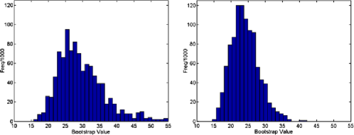
(a)

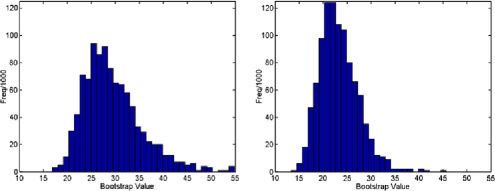
(b)

Figure 8: Bootstrap distributions for four randomly chosen scans, (a) two with changes detected, (b) two with no changes detected, when using 125 components and the sum-statistic $\widetilde{T}_{n}^{(A)}$. The distributions vary due to the differing temporal correlation structures for different individuals.

Figure 8 shows four typical examples of bootstrap distributions with and without changes detected. While differences due to the different underlying correlation structures are clearly visible, no difference is apparent between scans which contain a detected change and those which do not. Figure 9 shows the distribution of the 5% bootstrap critical values from 197 scans, once more indicating that the critical values show some deviation between scans due to different underlying correlation structures, hence different limit distributions, but do not differ between those with or without changes detected.

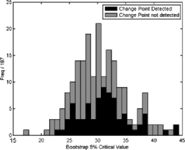
Figure 9: Distribution of bootstrap 5% critical values from 197 scans, where the stacking shows whether the critical value was from a scan with detected or no detected change using 125 components and the sum-statistic $\widetilde{T}_{n}^{(A)}$.

After the preprocessing of the data described in Section 2, a separable functional principal component decomposition was found, based on the three orthogonal directions within the image acquisition. Eigen-decompositions of the empirical covariance functions were used to generate the full three-dimensional functional basis. The eigenvalues associated with the decompositions did not decrease particularly fast. Indeed, the first 1000 eigenvalues only explained approximately 5% of the variation. In many applications, this is unappealing as it means that the data cannot be sparsely represented. However, in change-point detection, a flat eigenstructure in the uncontaminated covariance can actually (and somewhat counter-intuitively) enhance detectability and is therefore actually an advantageous property. By Corollary 5.1, change-points, if present, will tend to be found in eigenfunctions with larger relative eigenvalues, and hence only a small number of components need to be checked, especially when the components are flat. Thus, the number of components to examine was set to a small number, namely, systems with 64 ($=4^{3}$) and 125 ($=5^{3}$) eigenfunctions were investigated, with each direction having either its top 4 or 5 eigenfunctions as part of the tensor product. This was a compromise between having a large number of components, which would reduce the finite sample detectability as well as computational speed (processing time in Matlab for one scan with 1000 bootstrap samples for 125 components was approximately 6–7 hours on a desktop PC, while processing for the entire 197 scans took approximately 24 hours on a 40 node cluster), and having a sufficient number of components not to miss possible changes. Since the original data set was of dimension $64\times 64\times 33$, systems with 64 and 125 eigenfunctions correspond to an approximate dimension reduction by a factor of 2000 or 1000, respectively. Three examples of the projected data of dimension 64 were discussed in Section 4.

The test statistics $\widetilde{T}_{n}^{(A/B)}$ in (6.1) were found for all 197 scans for a change-point. Bootstrap resampling as described in Section 6.2 was used to obtain critical values for each time series ($M=1000$). Multiple comparisons were corrected controlling the FDR by the procedure of Benjamini and Hochberg (1995) for independent observations. In this case, unlike in usual brain imaging applications, the correction is done across subjects, not across space, as here space is a single functional observation, while different subjects can be deemed independent.

Table 2: Results of the 64 and 125 component analyses. “No correction” indicates all rejections at the 5% level were counted, while “FDR correction” indicates FDR correction was used at a 5% level, with the corresponding threshold being given

Number of		Rejections	Rejections
components	Statistic used	(no correction)	(FDR correction)	FDR thresh
64	max($\widetilde{T}_{n}^{(B)}$)	088	085	0.025
	sum($\widetilde{T}_{n}^{(A)}$)	078	070	0.022
125	max($\widetilde{T}_{n}^{(B)}$)	109	107	0.029
	sum($\widetilde{T}_{n}^{(A)}$)	082	076	0.022

The test results are summarized in Table 2. There was not a large difference whether 64 or 125 components were chosen, particularly for the sum statistic. Indeed, a small number of subjects became insignificant when 125 components instead of 64 components were used, while others became significant. Therefore, the results look fairly stable regardless of the number of components chosen. If the sum statistic is used, approximately 40% of all subjects in the study were found to have some form of nonstationarity present, which resulted in their being rejected as stationary against an epidemic alternative.

7.1 Comparison of results to exponentially weighted moving average method

An alternative method for determining change-points is that given by Lindquist, Waugh and Wager (2007) where an exponentially weighted moving average (EWMA) scheme is adopted. This is based on control chart theory and uses control limits to determine periods of switching between states. The method has been shown to be particularly appropriate in tasks where activations take place, but where the times of onset and duration are not known.

The methodology has two principle differences from the approach adopted in this paper. First, it is a voxelwise approach as opposed to a functional approach. This means that each voxel is tested individually. While this has the obvious advantage of being able to determine on a voxel by voxel basis if changes occur, it has the disadvantage that multiple comparisons need to be taken into account, and also the times of changes need not be similar even among neighboring voxels, yielding difficulties in interpretation. The second major distinction is that the approach requires a parametric model for the error structure, as opposed to the nonparametric approach within the method proposed in this paper. The choice of error structure is known to affect the detection of change-points if incorrectly specified, and indeed has been shown to be problematic for fMRI time series in particular [see, e.g., Nam, Aston and Johansen (2012)].

Resting state data is inherently different from activation data and the model for the noise will be inherently more important in this case, in that no activation is expected to take place. As can be seen in Figure 10, depending on whether a white noise, AR(1) or ARMA($1,1$)

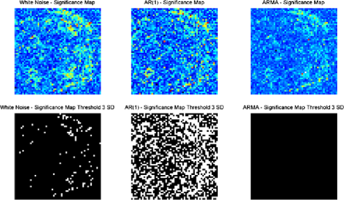
Figure 10: Results for three different noise model assumptions for the EWMA method as applied to subject 01018 (view of plane 15). The top row shows the significance maps for white noise, $\operatorname{AR}(1)$ errors and $\operatorname{ARMA}(1,1)$ errors, respectively, while the bottom row shows those voxels which would be deemed significant at a threshold of 3 standard deviations. As can be seen, the results of the method depend considerably on the noise model chosen.

model is chosen, the number of change-points within the image varies considerably, despite the same threshold being applied. The same analysis using the methodology proposed in this paper resulted in nonstationarities being detected (see Figure 3). The differences in the EWMA analysis for alternative noise models are likely due to the difficulty in expressing the noise structure accurately for resting state data, in comparison to activation-baseline tasks where AR(1) and ARMA($1,1$) type noise structures are known to be fairly good approximations.

8 Distribution of the position and duration of the epidemic change

The discussion in the previous sections has dealt with situations where one functional time series is observed and for this time series the question arises if and when a change has occurred. In some situations, such as in psychological experiments or in stress testing, due to the design of the experiment [cf., e.g., Lindquist, Waugh and Wager (2007)], one can be reasonably sure that a certain change will occur. Usually in such situations more than one time series, namely, one time series for each person involved in the experiment, is observed. Therefore, it makes sense to include the change-point in the model and estimate the density of the change-point. For example, one may be interested in knowing the distribution of the change-point in stress testing to get an idea about the change and duration distribution.

8.1 Density estimation of the change-point for hierarchical time-series

Before giving technical details, let us summarize the results of this subsection as follows. First, it is possible to show that even if we use the estimated change-point as derived earlier instead of the true change-point, the empirical distribution function (EDF) and the kernel density estimate (KDE) of the joint epidemic change-point location and duration both remain consistent. In the case of fMRI, this allows us to take the change-points positions from each subject and combine them to give a population based distribution of the times of changes that occur in the scanner. By showing that both the EDF and KDE are valid means that either a histogram based approach or a smooth density approach can be used as required. As the change-points are functions of time, they can be combined across subjects without requiring spatial normalization, because the distributions are independent of the spatial location of the change. In fact, there may be many different causes of a nonstationary change in the data, with the question arising as to whether these might have consistent timings within the scanning period.

In the remainder of the section we give the results for EDFs and KDEs in full statistical details. Those readers most interested in the results of such estimates for fMRI resting scan data could proceed to Section 8.2 where the data analysis is detailed.

Let in case of AMOC

$$X_{t,j}(u)=Y_{t,j}(u)+\mu_{j}(u)+\Delta_{j}(u)1_{\{t>\vartheta_{j}n\}},\qquad 1\leq t\leq n,1\leq j\leq m,$$

where the $m$ observed functional time series $\{X_{t,1}\dvtx 1\leq t\leq n\},\ldots,\{X_{t,m}\dvtx 1\leq t\leq n\}$ are independent, $\{{{\bolds{\mu}}_{j}}\dvtx 1\leq j\leq m\}$, $\{\bolds{\Delta}_{j}\dvtx 1\leq j\leq m\}$, and $\{\vartheta_{j}\dvtx 1\leq j\leq m\}$ are no longer fixed deterministic but rather i.i.d. random variables independent of $\{Y_{t,j}(\cdot)\dvtx t\geq 1\},j=1,\ldots,m$, $P(0<\vartheta_{1}<1)=1$ and $P(\bolds{\Delta}_{1}\equiv 0)=0$. For each fixed $j$, the model is still as before, and the index $j$ indicates the person to whom the observation belongs.

Furthermore, we assume $n=n(m)\to\infty$ as $m\to\infty$.

Denoting $P^{*}(\cdot)=P(\cdot|\vartheta_{j},{\bolds{\mu}_{j}},{\bolds{\Delta}_{j}},j=1,\ldots,m)$, the consistency property $|\widehat{\vartheta}-\vartheta|=o_{P}(1)$ of AMOC estimators [cf. Theorem 2.3 in Aston and Kirch (2012b)] in the standard setting as outlined in Section 4.1 translates into

$$|\vartheta_{j}-\widehat{\vartheta}_{j}|=o_{P^{*}}(1)\qquad\mbox{a.s.}$$ (35)

if the assumptions are a.s. fulfilled, that is, the mean changes are a.s. nonorthogonal to the contaminated projection subspace and the basis is an orthonormal system almost surely.

Theorem 8.1

If (35) holds and the distribution function $F_{\vartheta}$ of $\vartheta$ is continuous, then

$$\widehat{F}_{\widehat{\vartheta},m}(x):=\frac{1}{m}\sum_{j=1}^{m}1_{\{\widehat{\vartheta}_{j}\leq x\}}$$

is a consistent estimator for $F_{\vartheta}$, that is,

$$\sup_{x\in[0,1]}\bigl{|}\widehat{F}_{\widehat{\vartheta},m}(x)-F_{\vartheta}(x)\bigr{|}\to 0\qquad\mbox{a.s.}$$

The following theorem gives a corresponding result for kernel density estimators if a rate for the estimators of the change-point [analogously to (22)] is available.

Theorem 8.2

Let $h=h(m)\to 0,hm\to\infty$ as $m\to\infty$. Assume

$$h^{-1}|\vartheta_{j}-\widehat{\vartheta}_{j}|=o_{P^{*}}(1)\qquad\mbox{a.s.},$$ (36)

which follows, for example, from the analogue of (22) if $h^{2}n\to\infty$. Let $K(\cdot)$ be a bounded and Lipschitz continuous kernel [$K(\cdot)\geq 0$, $\int K(x)\,dx=1$], then

$$\int\mathrm{E}\bigl{|}\widehat{f}_{\widehat{\vartheta},m}(x)-\widehat{f}_{m}(x)\bigr{|}^{2}\,dx\to 0,$$

where

$$\widehat{f}_{\widehat{\vartheta},m}(x)=\frac{1}{mh}\sum_{i=1}^{m}K\biggl{(}\frac{x-\widehat{\vartheta}_{i}}{h}\biggr{)}$$

and

$$\widehat{f}_{m}(x)=\frac{1}{mh}\sum_{i=1}^{m}K\biggl{(}\frac{x-{\vartheta}_{i}}{h}\biggr{)}$$

is the standard kernel estimator of the density $f_{\vartheta}$ of $\vartheta$.

The theorem shows, in particular, that under standard assumptions on the kernel and the density it holds

$$\int\mathrm{E}\bigl{|}\widehat{f}_{\widehat{\vartheta},m}(x)-f_{\vartheta}(x)\bigr{|}^{2}\,dx\to 0.$$

Remark 8.1.

For the univariate problem one can show

$$P\bigl{(}|\widehat{\vartheta}-\vartheta|\geq c_{n}\bigr{)}\leq C\bigl{(}\min(\vartheta,1-\vartheta)\bigr{)}^{-2}\Delta^{-2}n^{-1}c_{n}^{-1},$$

where $C$ does not depend on $\vartheta$ or $\mu,\Delta$; cf., for example, Kokoszka and Leipus (1998). If additionally $\mathrm{E}[\Delta^{-2}\min(\vartheta_{1},1-\vartheta_{1})^{-2}]<\infty$, then using the Markov-inequality and similar arguments as in the proof of the above theorem, one can conclude

$$\sup_{x}\bigl{|}f_{\widehat{\vartheta},m}(x)-\widehat{f}_{m}(x)\bigr{|}\to 0\qquad\mbox{a.s.},$$

if, for example, $nh^{3},mh^{3}\to\infty$. This shows that in this situation under standard assumptions it holds $\sup_{x}|f_{\widehat{\vartheta}}(x)-f_{\vartheta}(x)|\to 0$ a.s.

If we are interested in estimators for an epidemic change, things become slightly more complicated. The above results carry over immediately to $\widehat{\vartheta}_{i}=\widehat{\vartheta}_{1i}$ as an estimator for the first change-point as well as to $\widehat{\tau}_{i}=\widehat{\vartheta}_{2i}-\widehat{\vartheta}_{1i}$ as an estimator for the duration of the epidemic change, so the marginal distributions can be estimated this way. This gives the joint distribution if one assumes that the first change-point ${\vartheta}_{1i}$ and the duration of the epidemic change ${\tau}_{i}$ are independent [as, e.g., done by Lindquist, Waugh and Wager (2007)]. If one does not want to make this assumption, one can formulate an analogous result using a two-dimensional kernel $K(x,y)$, that is, $\int K(x,y)\,dx\,dy=1$, that is positive and bounded, and fulfills the following Lipschitz condition

$$\bigl{|}K(x_{1},y_{1})-K(x_{2},y_{2})\bigr{|}\leq C\max\bigl{(}|x_{1}-x_{2}|,|y_{1}-y_{2}|\bigr{)}$$

for some $C>0$. Then, if $mh_{1}h_{2}\to\infty$, $h_{1},h_{2}\to 0$, one gets an analogous result as in Theorem 8.2 for

$$\widehat{f}_{\widehat{\vartheta}_{i},\widehat{\tau}_{i},m}(x,y) = \frac{1}{mh_{1}h_{2}}\sum_{i=1}^{m}K\biggl{(}\frac{x-\widehat{\vartheta}_{i}}{h_{1}},\frac{y-\widehat{\tau}_{i}}{h_{2}}\biggr{)},$$

$$\widehat{f}_{m}(x,y) = \frac{1}{mh_{1}h_{2}}\sum_{i=1}^{m}K\biggl{(}\frac{x-{\vartheta}_{i}}{h_{1}},\frac{y-{\tau}_{i}}{h_{2}}\biggr{)}.$$

The proof is analogous to the proof of Theorem 8.2.

8.2 Estimation for the connectome resting state data

The results in the previous section can now be applied for the subjects that survived the FDR threshold as outlined in Section 7, and the joint distribution of position and duration of the epidemic change can be derived.

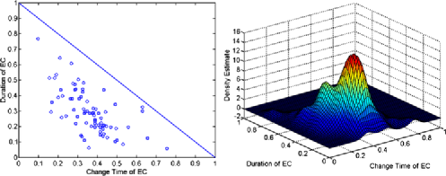
Figure 11: Estimators for 76 fMRI scans surviving FDR correction based on 125 components and the sum statistic $\widetilde{T}_{n}^{(A)}$. Left: joint estimates of position and duration of epidemic change. Right: kernel density estimate using a Gaussian kernel and bandwidths $h_{x}=0.04,h_{y}=0.05$.

The left panel in Figure 11 shows the estimated change and durations for all those subjects where the null hypothesis of no change was rejected using FDR, while the right panel shows a kernel smoothed density estimate for the joint distribution of position and duration of the epidemic change, using the automatic bandwidth selection procedure of Botev, Grotowski and Kroese (2010) (yielding bandwidths of $h_{x}=0.04$ and $h_{y}=0.05$). In this example change-points usually occur somewhere between 0.25 and 0.5, and last around 0.1–0.3 of the scanning period except for very early changes which often last longer. In fact, the density seems to be bimodal, indicating two clusters dividing subjects into those for which a change occurs after a relatively short period in the scanner (maybe only now arriving in the stationary state) in addition to a relatively long duration (possibly until the end of the scan), and those subjects for which after a short time in the epidemic state a return to baseline happens. However, for subjects with a relatively late change, a long duration cannot happen due to the limited time in the scanner. Therefore, the two modes may be an artifact of the statistical procedure based on the short time span.

The results of the study show that resting state scans in some cases do show evidence of deviation from stationarity which can be modeled by epidemic mean changes, at least as a first approximation, indicating that the overall activity is different at different times. This result has implications for studying correlations within the brain between regions of interest using multiple subjects, particularly if some subjects show nonstationary behavior, while others do not.

9 Conclusions

In this paper a methodology for the detection and estimation of change-points from multiple subjects has been outlined, and the associated statistical properties investigated. It has been shown that change-point analysis is a useful tool in situations where very high-dimensional data sets are collected across time, especially if the data have a natural spatial structure. One main result explains the impact of the choice of projection subspace estimation on the power of the tests. In particular, any structural breaks present will likely be found within the first few components when the eigenspectrum is relatively flat if one uses estimated principal components for the projection. The second main result shows that consistent estimators for the change-points exist and the associated distribution of change-point locations and durations can be found.

The main aim of this paper was to find a general framework for the testing and estimation of change-points in resting state fMRI data, in such a way that details such as the estimation procedure for the projection subspace can be replaced with different statistical techniques while the underlying theoretical results remain valid. Examples include methodology based on fixed spatial basis choices such as wavelets, or computational methods such as those by Zipunnikov et al. (2011) extended to time series settings. For these variations, by careful choice of the estimators for the projection subspace, tests as well as estimators for the location and duration distributions can be obtained from the theoretic results given in this paper.

For resting state fMRI data, the covariance function $c$ is probably one of the most important quantities of interest. Indeed, the full function would give a complete connectivity map for the brain. However, due to its inherent size, connectivity studies take approximations or subsets of this function and use these to derive models for the default network, for example. However, as we have seen in the theoretical analysis, when nonstationarities are present, we do not observe $c$ but rather the contaminated version $k$, that is, the connectivity map but also elements associated with nonstationarities. As there is no inherent reason to believe these nonstationarities are anything other than subject specific, they will induce false correlations not related to the true underlying connectivity in a standard correlation based analysis to derive connectivity measures. However, by performing tests such as those we have derived, it is at least now possible to pick candidate subjects with no evidence of nonstationarities, or alternatively investigate further the causes of the nonstationarities in those with evidence of such changes, in case they are intrinsically part of the default network in multiple subjects.

It should be noted that while we have used tests and estimators designed for epidemic changes in this paper, it is likely that other forms of nonstationarity might be present in applications such as fMRI, as well as possible multiple epidemic changes. However, the use of epidemic changes is a good first approximation as it not only mimics the most likely form of nonstationarity present in fMRI but will also have power against other alternatives too, including multiple epidemic changes as well as slow transient changes (where instead of a jump up or jump back, this takes some amount of time). Of course, the detection will not be optimal in these cases, but detection is still likely for reasonable sized changes. It is for this reason that we feel that it would be unwise to draw too many conclusions from the actual maps that could be generated for $\Delta(u)$ based on the epidemic change alternative. However, because of this, neuroscientific conclusions should really be restricted to those which can be based on the timings of changes, with further investigation being required, to account for possible effects such as hemodynamic lag, to draw conclusions concerning any underlying neuronal changes.

While the estimators and tests can be used in many applications, from epidemics to image based security surveillance, the application that drove all the theoretical developments was resting state fMRI. As a result, for future statistical analyses of resting state fMRI data, this study has three main implications:

• First, routine testing for nonstationarities in resting-state scans is now possible, and relatively computationally inexpensive (compared to the time taken to do further analyses).

• Second, this study indicates that the examined subjects are fairly well split between those that have evidence of nonstationarities and those who do not, so that it would be of great interest to compare the connectivity relationships between these two groups. Many of the most standard connectivity measures are based on correlation analyses, which can be dramatically affected by the presence of nonstationarities. Hence, investigation of the phenomena found in this paper warrants further exploration.

• Third, the distributions derived from the change-point estimators seem to indicate that the location and duration of the nonstationarities have considerable mass around half way through the scan. This position (in contrast to the test result) could be a statistical artifact, in that while the test itself reveals the presence of nonstationarity, the type of nonstationarity might not be epidemic, but the epidemic change hypothesis could still be powerful against evidence of stationarity. It would thus be of interest to investigate further whether this nonstationary behavior is due to the ability or inability to rest within the scanner and is due to active thought processes interrupting the resting state network, or whether the resting state signal itself changes after a certain amount of time. This could be investigated by looking at the spatial distribution of the time series which exhibit changes, but requires further statistical development to rigorously allow the examination of individual spatial maps after the omnibus test for the presence of an epidemic change.

References

- Aston and Gunn (2005) {barticle}[mr] \bauthor\bsnmAston, \bfnmJohn A. D.\binitsJ. A. D. and \bauthor\bsnmGunn, \bfnmRoger N.\binitsR. N. (\byear2005). \btitleStatistical estimation with Kronecker products in positron emission tomography. \bjournalLinear Algebra Appl. \bvolume398 \bpages25–36. \biddoi=10.1016/j.laa.2003.11.018, issn=0024-3795, mr=2121342 \bptokimsref \endbibitem
- Aston and Kirch (2012a) {barticle}[author] \bauthor\bsnmAston, \bfnmJ. A. D.\binitsJ. A. D. and \bauthor\bsnmKirch, \bfnmC.\binitsC. (\byear2012a). \btitleSupplement to “Evaluating stationarity via change-point alternatives with applications to fMRI data.” DOI:10.1214/ 12-AOAS565SUPP. \bptokimsref \endbibitem
- Aston and Kirch (2012b) {barticle}[author] \bauthor\bsnmAston, \bfnmJ. A. D.\binitsJ. A. D. and \bauthor\bsnmKirch, \bfnmC.\binitsC. (\byear2012b). \btitleDetecting and estimating changes in dependent functional data. \bjournalJ. Multivariate Anal. \bvolume109 \bpages204–220. \bptokimsref \endbibitem
- Aston et al. (2005) {barticle}[author] \bauthor\bsnmAston, \bfnmJ. A. D.\binitsJ. A. D., \bauthor\bsnmGunn, \bfnmR. N.\binitsR. N., \bauthor\bsnmHinz, \bfnmR.\binitsR. and \bauthor\bsnmTurkheimer, \bfnmF. E.\binitsF. E. (\byear2005). \btitleWavelet variance components in image space for spatiotemporal neuroimaging data. \bjournalNeuroimage \bvolume25 \bpages159–168. \bptokimsref \endbibitem
- Aue et al. (2009) {barticle}[mr] \bauthor\bsnmAue, \bfnmAlexander\binitsA., \bauthor\bsnmGabrys, \bfnmRobertas\binitsR., \bauthor\bsnmHorváth, \bfnmLajos\binitsL. and \bauthor\bsnmKokoszka, \bfnmPiotr\binitsP. (\byear2009). \btitleEstimation of a change-point in the mean function of functional data. \bjournalJ. Multivariate Anal. \bvolume100 \bpages2254–2269. \biddoi=10.1016/j.jmva.2009.04.001, issn=0047-259X, mr=2560367 \bptokimsref \endbibitem
- Beckmann and Smith (2005) {barticle}[pbm] \bauthor\bsnmBeckmann, \bfnmC. F.\binitsC. F. and \bauthor\bsnmSmith, \bfnmS. M.\binitsS. M. (\byear2005). \btitleTensorial extensions of independent component analysis for multisubject FMRI analysis. \bjournalNeuroimage \bvolume25 \bpages294–311. \biddoi=10.1016/j.neuroimage.2004.10.043, issn=1053-8119, pii=S1053-8119(04)00637-8, pmid=15734364 \bptokimsref \endbibitem
- Beckmann et al. (2005) {barticle}[author] \bauthor\bsnmBeckmann, \bfnmC. F.\binitsC. F., \bauthor\bsnmDeLuca, \bfnmM.\binitsM., \bauthor\bsnmDevlin, \bfnmJ. T.\binitsJ. T. and \bauthor\bsnmSmith, \bfnmS. M.\binitsS. M. (\byear2005). \btitleInvestigations into resting-state connectivity using independent component analysis. \bjournalPhilosophical Transactions of the Royal Society B: Biological Sciences \bvolume360 \bpages1001–1013. \bptokimsref \endbibitem
- Benjamini and Hochberg (1995) {barticle}[mr] \bauthor\bsnmBenjamini, \bfnmYoav\binitsY. and \bauthor\bsnmHochberg, \bfnmYosef\binitsY. (\byear1995). \btitleControlling the false discovery rate: A practical and powerful approach to multiple testing. \bjournalJ. Roy. Statist. Soc. Ser. B \bvolume57 \bpages289–300. \bidissn=0035-9246, mr=1325392 \bptokimsref \endbibitem
- Berkes et al. (2009) {barticle}[mr] \bauthor\bsnmBerkes, \bfnmIstván\binitsI., \bauthor\bsnmGabrys, \bfnmRobertas\binitsR., \bauthor\bsnmHorváth, \bfnmLajos\binitsL. and \bauthor\bsnmKokoszka, \bfnmPiotr\binitsP. (\byear2009). \btitleDetecting changes in the mean of functional observations. \bjournalJ. R. Stat. Soc. Ser. B Stat. Methodol. \bvolume71 \bpages927–946. \biddoi=10.1111/j.1467-9868.2009.00713.x, issn=1369-7412, mr=2750251 \bptokimsref \endbibitem
- Biswal et al. (2010) {barticle}[author] \bauthor\bsnmBiswal, \bfnmBharat B.\binitsB. B. \betalet al. (\byear2010). \btitleToward discovery science of human brain function. \bjournalProc. Natl. Acad. Sci. USA \bvolume107 \bpages4734–4739. \bptokimsref \endbibitem
- Bosq (2000) {bbook}[mr] \bauthor\bsnmBosq, \bfnmD.\binitsD. (\byear2000). \btitleLinear Processes in Function Spaces: Theory and Applications. \bseriesLecture Notes in Statistics \bvolume149. \bpublisherSpringer, \baddressNew York. \biddoi=10.1007/978-1-4612-1154-9, mr=1783138 \bptokimsref \endbibitem
- Botev, Grotowski and Kroese (2010) {barticle}[mr] \bauthor\bsnmBotev, \bfnmZ. I.\binitsZ. I., \bauthor\bsnmGrotowski, \bfnmJ. F.\binitsJ. F. and \bauthor\bsnmKroese, \bfnmD. P.\binitsD. P. (\byear2010). \btitleKernel density estimation via diffusion. \bjournalAnn. Statist. \bvolume38 \bpages2916–2957. \biddoi=10.1214/10-AOS799, issn=0090-5364, mr=2722460 \bptokimsref \endbibitem
- Bullmore et al. (2003) {barticle}[mr] \bauthor\bsnmBullmore, \bfnmEd\binitsE., \bauthor\bsnmFadili, \bfnmJalal\binitsJ., \bauthor\bsnmBreakspear, \bfnmMichael\binitsM., \bauthor\bsnmSalvador, \bfnmRaymond\binitsR., \bauthor\bsnmSuckling, \bfnmJohn\binitsJ. and \bauthor\bsnmBrammer, \bfnmMichael\binitsM. (\byear2003). \btitleWavelets and statistical analysis of functional magnetic resonance images of the human brain. \bjournalStat. Methods Med. Res. \bvolume12 \bpages375–399. \biddoi=10.1191/0962280203sm339ra, issn=0962-2802, mr=2005443 \bptokimsref \endbibitem
- Cole, Smith and Beckmann (2010) {barticle}[author] \bauthor\bsnmCole, \bfnmD. M.\binitsD. M., \bauthor\bsnmSmith, \bfnmS. M.\binitsS. M. and \bauthor\bsnmBeckmann, \bfnmC. F.\binitsC. F. (\byear2010). \btitleAdvances and pitfalls in the analysis and interpretation of resting-state FMRI data. \bjournalFrontiers in System Neuroscience \bvolume4 \bpages1–15. \bptokimsref \endbibitem
- Damoiseaux et al. (2006) {barticle}[author] \bauthor\bsnmDamoiseaux, \bfnmJ. S.\binitsJ. S., \bauthor\bsnmRombouts, \bfnmS. A. R. B.\binitsS. A. R. B., \bauthor\bsnmBarkhof, \bfnmF.\binitsF., \bauthor\bsnmScheltens, \bfnmP.\binitsP., \bauthor\bsnmStam, \bfnmC. J.\binitsC. J., \bauthor\bsnmSmith, \bfnmS. M.\binitsS. M. and \bauthor\bsnmBeckmann, \bfnmC. F.\binitsC. F. (\byear2006). \btitleConsistent resting-state networks across healthy subjects. \bjournalProc. Natl. Acad. Sci. USA \bvolume103 \bpages13848–13853. \bptokimsref \endbibitem
- Diggle, Rowlingson and Su (2005) {barticle}[mr] \bauthor\bsnmDiggle, \bfnmPeter\binitsP., \bauthor\bsnmRowlingson, \bfnmBarry\binitsB. and \bauthor\bsnmSu, \bfnmTing-Li\binitsT.-L. (\byear2005). \btitlePoint process methodology for on-line spatio-temporal disease surveillance. \bjournalEnvironmetrics \bvolume16 \bpages423–434. \biddoi=10.1002/env.712, issn=1180-4009, mr=2147534 \bptokimsref \endbibitem
- Doucet et al. (2012) {barticle}[pbm] \bauthor\bsnmDoucet, \bfnmGaëlle\binitsG., \bauthor\bsnmNaveau, \bfnmMikaël\binitsM., \bauthor\bsnmPetit, \bfnmLaurent\binitsL., \bauthor\bsnmZago, \bfnmLaure\binitsL., \bauthor\bsnmCrivello, \bfnmFabrice\binitsF., \bauthor\bsnmJobard, \bfnmGaël\binitsG., \bauthor\bsnmDelcroix, \bfnmNicolas\binitsN., \bauthor\bsnmMellet, \bfnmEmmanuel\binitsE., \bauthor\bsnmTzourio-Mazoyer, \bfnmNathalie\binitsN., \bauthor\bsnmMazoyer, \bfnmBernard\binitsB. and \bauthor\bsnmJoliot, \bfnmMarc\binitsM. (\byear2012). \btitlePatterns of hemodynamic low-frequency oscillations in the brain are modulated by the nature of free thought during rest. \bjournalNeuroimage \bvolume59 \bpages3194–3200. \biddoi=10.1016/j.neuroimage.2011.11.059, issn=1095-9572, pii=S1053-8119(11)01341-3, pmid=22155378 \bptokimsref \endbibitem
- Dryden et al. (2009) {barticle}[mr] \bauthor\bsnmDryden, \bfnmIan L.\binitsI. L., \bauthor\bsnmBai, \bfnmLi\binitsL., \bauthor\bsnmBrignell, \bfnmChristopher J.\binitsC. J. and \bauthor\bsnmShen, \bfnmLinlin\binitsL. (\byear2009). \btitleFactored principal components analysis, with applications to face recognition. \bjournalStat. Comput. \bvolume19 \bpages229–238. \biddoi=10.1007/s11222-008-9087-6, issn=0960-3174, mr=2516216 \bptokimsref \endbibitem
- Dutilleul (1999) {barticle}[author] \bauthor\bsnmDutilleul, \bfnmP.\binitsP. (\byear1999). \btitleThe MLE algorithm for the matrix normal distribution. \bjournalJ. Stat. Comput. Simul. \bvolume64 \bpages105–123. \bptokimsref \endbibitem
- Ferraty and Vieu (2006) {bbook}[mr] \bauthor\bsnmFerraty, \bfnmFrédéric\binitsF. and \bauthor\bsnmVieu, \bfnmPhilippe\binitsP. (\byear2006). \btitleNonparametric Functional Data Analysis: Theory and Practice. \bpublisherSpringer, \baddressNew York. \bidmr=2229687 \bptokimsref \endbibitem
- Friston et al. (1993) {barticle}[author] \bauthor\bsnmFriston, \bfnmK. J.\binitsK. J., \bauthor\bsnmFrith, \bfnmC. D.\binitsC. D., \bauthor\bsnmLiddle, \bfnmP. F.\binitsP. F. and \bauthor\bsnmFrackowiak, \bfnmR. S. J.\binitsR. S. J. (\byear1993). \btitleFunctional connectivity: The principal-component analysis of large (PET) data sets. \bjournalJournal of Cerebral Blood Flow and Metabolism \bvolume13 \bpages5–14. \bptokimsref \endbibitem
- Fuentes (2006) {barticle}[mr] \bauthor\bsnmFuentes, \bfnmMontserrat\binitsM. (\byear2006). \btitleTesting for separability of spatial-temporal covariance functions. \bjournalJ. Statist. Plann. Inference \bvolume136 \bpages447–466. \biddoi=10.1016/j.jspi.2004.07.004, issn=0378-3758, mr=2211349 \bptnotecheck year\bptokimsref \endbibitem
- Genton (2007) {barticle}[mr] \bauthor\bsnmGenton, \bfnmMarc G.\binitsM. G. (\byear2007). \btitleSeparable approximations of space–time covariance matrices. \bjournalEnvironmetrics \bvolume18 \bpages681–695. \biddoi=10.1002/env.854, issn=1180-4009, mr=2408938 \bptokimsref \endbibitem
- Gohberg, Goldberg and Kaashoek (2003) {bbook}[mr] \bauthor\bsnmGohberg, \bfnmIsrael\binitsI., \bauthor\bsnmGoldberg, \bfnmSeymour\binitsS. and \bauthor\bsnmKaashoek, \bfnmMarinus A.\binitsM. A. (\byear2003). \btitleBasic Classes of Linear Operators. \bpublisherBirkhäuser, \baddressBasel. \biddoi=10.1007/978-3-0348-7980-4, mr=2015498 \bptokimsref \endbibitem
- Härdle and Simar (2007) {bbook}[mr] \bauthor\bsnmHärdle, \bfnmWolfgang\binitsW. and \bauthor\bsnmSimar, \bfnmLéopold\binitsL. (\byear2007). \btitleApplied Multivariate Statistical Analysis, \bedition2nd ed. \bpublisherSpringer, \baddressBerlin. \bidmr=2367300 \bptokimsref \endbibitem
- Hörmann and Kokoszka (2010) {barticle}[mr] \bauthor\bsnmHörmann, \bfnmSiegfried\binitsS. and \bauthor\bsnmKokoszka, \bfnmPiotr\binitsP. (\byear2010). \btitleWeakly dependent functional data. \bjournalAnn. Statist. \bvolume38 \bpages1845–1884. \biddoi=10.1214/09-AOS768, issn=0090-5364, mr=2662361 \bptokimsref \endbibitem
- Horváth and Kokoszka (2012) {bbook}[author] \bauthor\bsnmHorváth, \bfnmL.\binitsL. and \bauthor\bsnmKokoszka, \bfnmP.\binitsP. (\byear2012). \btitleInference for Functional Data with Applications. \bpublisherSpringer, \baddressNew York. \bptokimsref \endbibitem
- Hušková and Kirch (2008) {barticle}[mr] \bauthor\bsnmHušková, \bfnmMarie\binitsM. and \bauthor\bsnmKirch, \bfnmClaudia\binitsC. (\byear2008). \btitleBootstrapping confidence intervals for the change-point of time series. \bjournalJ. Time Series Anal. \bvolume29 \bpages947–972. \biddoi=10.1111/j.1467-9892.2008.00589.x, issn=0143-9782, mr=2464948 \bptokimsref \endbibitem
- Hušková and Kirch (2010) {barticle}[mr] \bauthor\bsnmHušková, \bfnmMarie\binitsM. and \bauthor\bsnmKirch, \bfnmClaudia\binitsC. (\byear2010). \btitleA note on Studentized confidence intervals for the change-point. \bjournalComput. Statist. \bvolume25 \bpages269–289. \biddoi=10.1007/s00180-009-0175-7, issn=0943-4062, mr=2639810 \bptokimsref \endbibitem
- Jenkinson et al. (2002) {barticle}[author] \bauthor\bsnmJenkinson, \bfnmM.\binitsM., \bauthor\bsnmBannister, \bfnmP. R.\binitsP. R., \bauthor\bsnmBrady, \bfnmJ. M.\binitsJ. M. and \bauthor\bsnmSmith, \bfnmS. M.\binitsS. M. (\byear2002). \btitleImproved optimisation for the robust and accurate linear registration and motion correction of brain images. \bjournalNeuroImage \bvolume17 \bpages825–841. \bptokimsref \endbibitem
- Kirch (2006) {bmisc}[author] \bauthor\bsnmKirch, \bfnmC.\binitsC. (\byear2006). \bhowpublishedResampling methods for the change analysis of dependent data. Ph.D. thesis, Univ. Cologne, Cologne. Available at http://kups.ub.uni-koeln.de/volltexte/ 2006/1795/. \bptokimsref \endbibitem
- Kirch (2007) {barticle}[mr] \bauthor\bsnmKirch, \bfnmClaudia\binitsC. (\byear2007). \btitleBlock permutation principles for the change analysis of dependent data. \bjournalJ. Statist. Plann. Inference \bvolume137 \bpages2453–2474. \biddoi=10.1016/j.jspi.2006.09.026, issn=0378-3758, mr=2325449 \bptokimsref \endbibitem
- Kirch and Politis (2011) {barticle}[mr] \bauthor\bsnmKirch, \bfnmClaudia\binitsC. and \bauthor\bsnmPolitis, \bfnmDimitris N.\binitsD. N. (\byear2011). \btitleTFT-bootstrap: Resampling time series in the frequency domain to obtain replicates in the time domain. \bjournalAnn. Statist. \bvolume39 \bpages1427–1470. \biddoi=10.1214/10-AOS868, issn=0090-5364, mr=2850208 \bptokimsref \endbibitem
- Kokoszka and Leipus (1998) {barticle}[mr] \bauthor\bsnmKokoszka, \bfnmPiotr\binitsP. and \bauthor\bsnmLeipus, \bfnmRemigijus\binitsR. (\byear1998). \btitleChange-point in the mean of dependent observations. \bjournalStatist. Probab. Lett. \bvolume40 \bpages385–393. \biddoi=10.1016/S0167-7152(98)00145-X, issn=0167-7152, mr=1664564 \bptokimsref \endbibitem
- Lahiri (2003) {bbook}[mr] \bauthor\bsnmLahiri, \bfnmS. N.\binitsS. N. (\byear2003). \btitleResampling Methods for Dependent Data. \bpublisherSpringer, \baddressNew York. \bidmr=2001447 \bptokimsref \endbibitem
- Lindquist, Waugh and Wager (2007) {barticle}[pbm] \bauthor\bsnmLindquist, \bfnmMartin A.\binitsM. A., \bauthor\bsnmWaugh, \bfnmChristian\binitsC. and \bauthor\bsnmWager, \bfnmTor D.\binitsT. D. (\byear2007). \btitleModeling state-related fMRI activity using change-point theory. \bjournalNeuroimage \bvolume35 \bpages1125–1141. \biddoi=10.1016/j.neuroimage.2007.01.004, issn=1053-8119, pii=S1053-8119(07)00009-2, pmid=17360198 \bptokimsref \endbibitem
- Long et al. (2011) {barticle}[mr] \bauthor\bsnmLong, \bfnmChristopher J.\binitsC. J., \bauthor\bsnmPurdon, \bfnmPatrick L.\binitsP. L., \bauthor\bsnmTemereanca, \bfnmSimona\binitsS., \bauthor\bsnmDesai, \bfnmNeil U.\binitsN. U., \bauthor\bsnmHämäläinen, \bfnmMatti S.\binitsM. S. and \bauthor\bsnmBrown, \bfnmEmery N.\binitsE. N. (\byear2011). \btitleState-space solutions to the dynamic magnetoencephalography inverse problem using high performance computing. \bjournalAnn. Appl. Stat. \bvolume5 \bpages1207–1228. \biddoi=10.1214/11-AOAS483, issn=1932-6157, mr=2849772 \bptokimsref \endbibitem
- Mitchell, Genton and Gumpertz (2005) {barticle}[mr] \bauthor\bsnmMitchell, \bfnmMatthew W.\binitsM. W., \bauthor\bsnmGenton, \bfnmMarc G.\binitsM. G. and \bauthor\bsnmGumpertz, \bfnmMarcia L.\binitsM. L. (\byear2005). \btitleTesting for separability of space–time covariances. \bjournalEnvironmetrics \bvolume16 \bpages819–831. \biddoi=10.1002/env.737, issn=1180-4009, mr=2216653 \bptokimsref \endbibitem
- Morris et al. (2011) {barticle}[mr] \bauthor\bsnmMorris, \bfnmJeffrey S.\binitsJ. S., \bauthor\bsnmBaladandayuthapani, \bfnmVeerabhadran\binitsV., \bauthor\bsnmHerrick, \bfnmRichard C.\binitsR. C., \bauthor\bsnmSanna, \bfnmPietro\binitsP. and \bauthor\bsnmGutstein, \bfnmHoward\binitsH. (\byear2011). \btitleAutomated analysis of quantitative image data using isomorphic functional mixed models, with application to proteomics data. \bjournalAnn. Appl. Stat. \bvolume5 \bpages894–923. \biddoi=10.1214/10-AOAS407, issn=1932-6157, mr=2840180 \bptokimsref \endbibitem
- Nam, Aston and Johansen (2012) {bmisc}[author] \bauthor\bsnmNam, \bfnmC. F. H.\binitsC. F. H., \bauthor\bsnmAston, \bfnmJ. A. D\binitsJ. A. D. and \bauthor\bsnmJohansen, \bfnmA. M.\binitsA. M. (\byear2012). \bhowpublishedQuantifying uncertainty in change points. J. Time Series Anal. To appear. DOI:\doiurl10.1111/j.1467-9892.2011.00777.x. \bptokimsref \endbibitem
- Ogawa et al. (1990) {barticle}[author] \bauthor\bsnmOgawa, \bfnmS.\binitsS., \bauthor\bsnmLee, \bfnmT. M.\binitsT. M., \bauthor\bsnmKay, \bfnmA. R.\binitsA. R. and \bauthor\bsnmTank, \bfnmD. W.\binitsD. W. (\byear1990). \btitleBrain magnetic resonance imaging with contrast dependent on blood oxygenation. \bjournalProc. Natl. Acad. Sci. USA \bvolume87 \bpages9868–9872. \bptokimsref \endbibitem
- Page (1954) {barticle}[mr] \bauthor\bsnmPage, \bfnmE. S.\binitsE. S. (\byear1954). \btitleContinuous inspection schemes. \bjournalBiometrika \bvolume41 \bpages100–115. \bidissn=0006-3444, mr=0088850 \bptokimsref \endbibitem
- Politis (2011) {barticle}[author] \bauthor\bsnmPolitis, \bfnmD. N.\binitsD. N. (\byear2011). \btitleHigher-order accurate, positive semidefinite estimation of large-sample covariance and spectral density matrices. \bjournalEconometric Theory \bvolume27 \bpages703–744. \bptokimsref \endbibitem
- Ramsay and Silverman (2005) {bbook}[mr] \bauthor\bsnmRamsay, \bfnmJ. O.\binitsJ. O. and \bauthor\bsnmSilverman, \bfnmB. W.\binitsB. W. (\byear2005). \btitleFunctional Data Analysis, \bedition2nd ed. \bpublisherSpringer, \baddressNew York. \bidmr=2168993 \bptokimsref \endbibitem
- Robinson, Wager and Lindquist (2010) {barticle}[author] \bauthor\bsnmRobinson, \bfnmL. F.\binitsL. F., \bauthor\bsnmWager, \bfnmT. D.\binitsT. D. and \bauthor\bsnmLindquist, \bfnmM. A.\binitsM. A. (\byear2010). \btitleChange point estimation in multi-subject fMRI studies. \bjournalNeuroImage \bvolume49 \bpages1581–1592. \bptokimsref \endbibitem
- Ruttimann et al. (1998) {barticle}[pbm] \bauthor\bsnmRuttimann, \bfnmU. E.\binitsU. E., \bauthor\bsnmUnser, \bfnmM.\binitsM., \bauthor\bsnmRawlings, \bfnmR. R.\binitsR. R., \bauthor\bsnmRio, \bfnmD.\binitsD., \bauthor\bsnmRamsey, \bfnmN. F.\binitsN. F., \bauthor\bsnmMattay, \bfnmV. S.\binitsV. S., \bauthor\bsnmHommer, \bfnmD. W.\binitsD. W., \bauthor\bsnmFrank, \bfnmJ. A.\binitsJ. A. and \bauthor\bsnmWeinberger, \bfnmD. R.\binitsD. R. (\byear1998). \btitleStatistical analysis of functional MRI data in the wavelet domain. \bjournalIEEE Trans. Med. Imaging \bvolume17 \bpages142–154. \biddoi=10.1109/42.700727, issn=0278-0062, pmid=9688147 \bptokimsref \endbibitem
- Van Loan and Pitsianis (1993) {bincollection}[mr] \bauthor\bsnmVan Loan, \bfnmC. F.\binitsC. F. and \bauthor\bsnmPitsianis, \bfnmN.\binitsN. (\byear1993). \btitleApproximation with Kronecker products. In \bbooktitleLinear Algebra for Large Scale and Real-Time Applications (Leuven, 1992) (\beditor\bfnmM. S.\binitsM. S. \bsnmMoonen and \beditor\bfnmG. H.\binitsG. H. \bsnmGolub, eds.). \bseriesNATO Advanced Science Institutes Series E: Applied Sciences \bvolume232 \bpages293–314. \bpublisherKluwer Academic, \baddressDordrecht. \bidmr=1250183 \bptokimsref \endbibitem
- Vanhaudenhuyse et al. (2010) {barticle}[pbm] \bauthor\bsnmVanhaudenhuyse, \bfnmAudrey\binitsA., \bauthor\bsnmDemertzi, \bfnmAthena\binitsA., \bauthor\bsnmSchabus, \bfnmManuel\binitsM., \bauthor\bsnmNoirhomme, \bfnmQuentin\binitsQ., \bauthor\bsnmBredart, \bfnmSerge\binitsS., \bauthor\bsnmBoly, \bfnmMelanie\binitsM., \bauthor\bsnmPhillips, \bfnmChristophe\binitsC., \bauthor\bsnmSoddu, \bfnmAndrea\binitsA., \bauthor\bsnmLuxen, \bfnmAndre\binitsA., \bauthor\bsnmMoonen, \bfnmGustave\binitsG. and \bauthor\bsnmLaureys, \bfnmSteven\binitsS. (\byear2010). \btitleTwo distinct neuronal networks mediate the awareness of environment and of self. \bjournalJ. Cogn. Neurosci. \bvolume23 \bpages570–578. \biddoi=10.1162/jocn.2010.21488, issn=1530-8898, pmid=20515407 \bptokimsref \endbibitem
- Werner, Jansson and Stoica (2008) {barticle}[mr] \bauthor\bsnmWerner, \bfnmKarl\binitsK., \bauthor\bsnmJansson, \bfnmMagnus\binitsM. and \bauthor\bsnmStoica, \bfnmPetre\binitsP. (\byear2008). \btitleOn estimation of covariance matrices with Kronecker product structure. \bjournalIEEE Trans. Signal Process. \bvolume56 \bpages478–491. \biddoi=10.1109/TSP.2007.907834, issn=1053-587X, mr=2445531 \bptokimsref \endbibitem
- Worsley et al. (2002) {barticle}[author] \bauthor\bsnmWorsley, \bfnmK. J.\binitsK. J., \bauthor\bsnmLiao, \bfnmC. H.\binitsC. H., \bauthor\bsnmAston, \bfnmJ. A. D.\binitsJ. A. D., \bauthor\bsnmPetre, \bfnmV.\binitsV., \bauthor\bsnmDuncan, \bfnmG. H.\binitsG. H., \bauthor\bsnmMorales, \bfnmF.\binitsF. and \bauthor\bsnmEvans, \bfnmA. C.\binitsA. C. (\byear2002). \btitleA general statistical analysis for fMRI data. \bjournalNeuroimage \bvolume15 \bpages1–15. \bptokimsref \endbibitem
- Zipunnikov et al. (2011) {barticle}[author] \bauthor\bsnmZipunnikov, \bfnmV.\binitsV., \bauthor\bsnmCaffo, \bfnmB.\binitsB., \bauthor\bsnmCrainiceanu, \bfnmC.\binitsC., \bauthor\bsnmYousem, \bfnmD. M.\binitsD. M., \bauthor\bsnmDavatzikos, \bfnmC.\binitsC. and \bauthor\bsnmSchwartz, \bfnmB. S.\binitsB. S. (\byear2011). \btitleMultilevel functional principal component analysis for high-dimensional data. \bjournalJ. Comput. Graph. Statist. \bvolume20 \bpages852–873. \bptokimsref \endbibitem