Generalized Multiscale Finite Element Methods (GMsFEM)
Abstract
In this paper, we propose a general approach called Generalized Multiscale Finite Element Method (GMsFEM) for performing multiscale simulations for problems without scale separation over a complex input space. As in multiscale finite element methods (MsFEMs), the main idea of the proposed approach is to construct a small dimensional local solution space that can be used to generate an efficient and accurate approximation to the multiscale solution with a potentially high dimensional input parameter space. In the proposed approach, we present a general procedure to construct the offline space that is used for a systematic enrichment of the coarse solution space in the online stage. The enrichment in the online stage is performed based on a spectral decomposition of the offline space. In the online stage, for any input parameter, a multiscale space is constructed to solve the global problem on a coarse grid. The online space is constructed via a spectral decomposition of the offline space and by choosing the eigenvectors corresponding to the largest eigenvalues. The computational saving is due to the fact that the construction of the online multiscale space for any input parameter is fast and this space can be re-used for solving the forward problem with any forcing and boundary condition. Compared with the other approaches where global snapshots are used, the local approach that we present in this paper allows us to eliminate unnecessary degrees of freedom on a coarse-grid level. We present various examples in the paper and some numerical results to demonstrate the effectiveness of our method.
1 Introduction
1.1 Multiscale problems, the input-output relation, and the need for model reduction
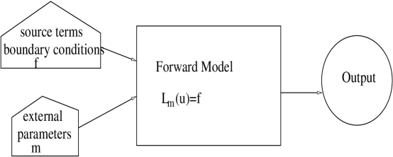
Many problems arising from various physical and engineering applications are multiscale in nature. Because of the presence of small scales and uncertainties in these problems, the direct simulations are prohibitively expensive. Moreover, these problems are typically solved for many source terms with input parameter coming from a high dimensional parameter space. For example, the flow in heterogeneous porous media described by Darcy’s equation is typically solved for multiple source terms. Moreover, the permeability usually has uncertainties which are parametrized in some sophisticated manner. In this case, one needs to solve many forward problems with different source terms and a wide range of permeabilities to make accurate predictions. These problems can be cast using an input-output relation (see Figure 1) which is typically done in reduced-order modeling. For the example of flow problems, the input space consists of source terms and the permeability that takes a value from a large parameter space. The output space depends on the quantities of interest and may consist of coarse-grid solutions or some other integrated quantities with respect to the solution. In many applications, the output space is typically smaller than the input space. The design of a general multiscale finite element framework that takes advantage of the effective low dimensional solution space for multiscale problems with high dimensional input space is the main objective of this paper.
Due to a large number of forward simulations, the computational effort can be tremendous to learn and process the output space given the high dimensionality of the input parameter space. In many of these problems, the solution space can be approximated by a low dimensional manifold via some model reduction tools. The main objective of reduced-order models is to represent the solution space with a small dimensional space. However, many existing reduced-order methods fail to give a small dimensional output solution space when the physical solution has multiscale structures. Another major limitation of the current reduced-order methods is that the reduced solution space needs to be regenerated for different forcing or boundary conditions. The general multiscale finite element framework proposed in this paper is designed to remove these two limitations by dividing the construction of reduced basis into the offline and online steps, and constructing our online multiscale bases from a reduced localized offline solution space.
1.2 Local and global model reduction concepts
Many local, global, and local-global model reduction techniques have been developed. The main idea of these methods is to find a small dimensional space that can represent the solution space given the input space.
Global model reduction techniques (see e.g., [39, 18, 6, 54]) construct a space of global fields that can approximate the solution space. One can, for example, consider a space of exhaustive global snapshots obtained by solving the global problem for many input parameters. This space can be further reduced using a spectral decomposition. In practice, the resulting space is constructed by solving global problems for some selected input parameters, right hand sides, and boundary conditions. These methods have been used with some success in practice. However, when the right hand sides or boundary conditions are changed, the resulting reduced space must be recomputed.
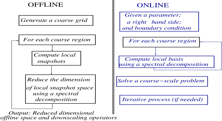
Local approaches (e.g., see [40, 43, 1, 3, 4, 7, 8, 20, 21, 33, 42] for upscaling and multiscale methods) attempt to approximate the solution in local (coarse-grid) regions for all input parameters without computing global snapshots of solutions. Local approaches first compute an offline space (possibly small dimensional) which is used to compute multiscale basis functions at the online stage. The local approximation space at the online stage is computed by finding a subspace of offline space for a given input parameter (see Figure 2).
Local approaches can be effective as they avoid the computation of global snapshots. Local approaches become more effective if the restriction of the solution space onto a local region has a small dimension. This is the case if the dimension of the space of solutions restricted to a coarse region is smaller than the dimension of the fine-grid space within this coarse region. For example, if the parameter is a coarse-grid scalar function, then at the coarse-grid level, this parameter is a scalar. While if we consider this problem from the point of view of a global model reduction, then the parameter belongs to a large dimensional space and this may not be amenable to computations.
One of advantages of local approaches is that they eliminate the unnecessary degrees of freedom in the parameter space at the coarse-grid level. In global methods, one first needs to compute many expensive global snapshots and many snapshots may not contribute to the solution at the online stage. In local approaches, these values of the parameter are identified at the coarse level inexpensively. Moreover, local approaches can easily handle large-scale parameter space when the parameter is a coarse-grid function and local approximation spaces are usually independent of the source terms or boundary conditions. We will further elaborate these issues in the paper.
1.3 This paper
In this paper, we introduce a general multiscale framework, which we call the Generalized Multiscale Finite Element Method (GMsFEM). This method incorporates complex input space information and the input-output relation. It systematically enriches the coarse space through our local construction. Our approach, as in many multiscale and model reduction techniques, divides the computation into two stages: offline; and online. In the offline stage, we construct a small dimensional space that can be efficiently used in the online stage to construct multiscale basis functions. These multiscale basis functions can be re-used for any input parameter to solve the problem on a coarse-grid. Thus, this provides a substantial computational saving at the online stage. Below, we present an outline of the algorithm and a chart that depicts our algorithm in Figure 2.
-
1.
Offline computation:
-
–
1.0. Coarse grid generation;
-
–
1.1. Construction of snapshot space that will be used to compute an offline space.
-
–
1.2. Construction of a small dimensional offline space by performing dimension reduction in the space of global snapshots.
-
–
-
2.
Online computations:
-
–
2.1. For each input parameter, compute multiscale basis functions;
-
–
2.2. Solution of a coarse-grid problem for any force term and boundary condition;
-
–
2.3. Iterative solvers, if needed.
-
–
In the offline computation, we first set up a coarse grid where each coarse-grid block consists of a connected union of fine-grid blocks. The construction of snapshot space in Step 1.1 involves solving local problems for various choices of input parameters. This space is used to construct the offline space in Step 1.2 via a spectral decomposition of the snapshot space. The snapshot space in a coarse region can be replaced by the fine-grid space associated with this coarse space; however, in many applications, one can judiciously choose the space of snapshots to avoid expensive offline space construction. The offline space in Step 1.2. is constructed by spectrally decomposing the space of snapshots. This spectral decomposition is typically based on the offline eigenvalue problem. The spectral decomposition enables us to select the high-energy elements from the offline space by choosing those eigenvectors corresponding to the largest eigenvalues. More precisely, we seek a subspace of the snapshot space such that it can approximate any element of the snapshot space in the appropriate sense defined via auxiliary bilinear forms.
In the online step 2.1, for a given input parameter, we compute the required online coarse space. In general, we want this to be a small dimensional subspace of the offline space. This space is computed by performing a spectral decomposition in the offline space via an eigenvalue problem. Furthermore, the eigenvectors corresponding to the largest eigenvalues are identified and used to form the online coarse space. The online coarse space is used within the finite element framework to solve the original global problem. Here, we propose several options such as the Galerkin coupling of multiscale basis functions, the Petrov-Galerkin coupling of multiscale basis functions, etc. In some of these coupling approaches, the choice of the initial partition of unity (that can be computed in the offline or online stage) is important and it will be discussed in the paper.
Our techniques differ from many previous approaches that are based on the homogenization theory. In the homogenization based methods, one usually constructs local approximation based on local solves and these approaches do not provide a systematic procedure to complement the local spaces. It is important to note that one needs to systematically complement the local spaces in order to converge to the fine-grid solution. How to develop an online systematic enrichment procedure and how to construct the initial partition of unity functions play a crucial role in obtaining a low dimensional offline space. These issues are central points of our proposed method.
We also discuss iterative solvers that use the coarse spaces and iterate on the residual to converge to the fine-scale solution. These iterative solvers serve as an online correction of the coarse-grid solution. We consider two-level domain decomposition preconditioners and some other methods where the importance of appropriately chosen multiscale coarse spaces has been demonstrated in the literature [53, 46]. We will discuss how the choice of coarse spaces yields optimal iterative solvers where the number of iterations is independent of the high contrast in the media properties.
2 A Generalized Multiscale Finite Element Method.
To describe the GMsFEM for linear problems, we consider
| (1) |
subject to some boundary conditions, where is the parameter. For example,
| (2) |
Here, the operator may depend on various spatial fields, e.g., heterogeneous conductivity fields, convection fields, reaction fields, and so on. The dependence of the solution from these fields is nonlinear, while the solution linearly depends on external source terms and boundary conditions. We assume there is a bilinear form associated with the operator that allows us to write the variational form of (1) in the form
| (3) |
for all test function and where is bilinear, coercive, and continuous for each , and is an inner product. We assume that is sufficiently smooth with respect to .
The proposed algorithms have advantages when has an affine representation defined as follows:
| (4) |
Here, are heterogeneous operators with multiple scales with the coefficients that have high contrast, the parameter is possibly a coarse-grid function and the functions . In terms of the corresponding bilinear form, we have
This affine representation allows pre-computing coarse-scale projections of in the offline stage and using them in the online stage. This reduces the computational cost considerably.
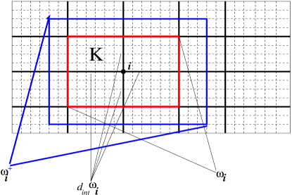
Before discussing the GMsFEM, we introduce the notion of a coarse grid. Let be a usual conforming partition of into finite elements (triangles, quadrilaterals, tetrahedrahals,…). We call this partition the coarse grid and assume that this coarse grid is partitioned into fine-grid blocks. Each coarse-grid block is a connected union of fine-grid blocks. We denote by the number of coarse nodes, by the vertices of the coarse mesh and define the neighborhood of the node by
| (5) |
(see Figure 4).
The GMsFEM has a structure similar to that of MsFEM. The main difference between the two approaches is that we systematically enrich coarse spaces in GMsFEM and generalize it by considering an input space consisting of parameters and source terms. In the first step of GMsFEM (offline stage), we construct the space of ‘snapshots’, , a large dimensional space of local solutions. In the next step of the offline computation, we reduce the space via some spectral procedure to . In the second stage (online stage), for each input parameter, we construct a corresponding local space, that is used to solve the problem at the online stage for the given input parameter. Our systematic approach allows us to increase the dimension of the coarse space and achieve a convergence.
2.1 An illustrative example
Before presenting details of GMsFEM, we will present a simple example demonstrating the main concept of GMsFEM. We consider
on and assume , where and are pre-defined constants. We assume the interval is divided into equal regions .
As for the space of snapshots, , we can consider
on . Here, are some set of functions defined on , e.g., unit source terms. We can also consider the space of fine-grid functions within as the space of snapshots.
As for offline space, , we perform a spectral decomposition of the space of snapshots. We re-numerate the snapshot functions in by . We consider
where are some weights. Here, , and . The choices for the matrix will be discussed later. To generate the offline space, , we choose the largest eigenvalues (see later discussions on ) of
and find the corresponding eigenvectors in the space of by multiplication, , where are coordinates of the vector . Note that the offline space is computed across all ,…, . More precisely, if we reorder the snapshot functions using a single index based on the decay of eigenvalues to create the matrices
then
where and denote fine-scale matrices corresponding to the stiffness and mass matrices with the permeability . One can use modified in the computation of the mass matrix (see [30]).
To compute the online space for a given (the value around which the global problem is linearized), we consider an eigenvalue problem in . Let us denote the basis of by . We consider a spectral decomposition of via
To generate the online space, , we choose the largest eigenvalues of
and find the corresponding eigenvectors in the space of by multiplication, , where are coordinates of the vector , denote these basis functions by . More precisely, if we reorder the offline functions using a single index based on the decay of eigenvalues to create the matrices
that are defined on the fine grid, then
where and denote fine scale matrices corresponding to the stiffness and mass matrices.
At the final stage, these basis functions in each will be coupled via a global formulation, e.g., Galerkin formulation. In this case, the eigenfunctions are multiplied by the partition of unity functions to obtain a conforming basis. In this nonlinear example, one can use an iterative Picard iteration at the previous value of the solution , and in each iteration, a global problem is solved with for the value of averaged over a coarse block.
2.2 Step 1. Local multiscale basis functions (offline stage)
1.1. Generating snapshots
We call the local spatial fields (or local solutions ) as “local snapshots”. These local spatial fields are used to construct the offline space. This space consists of spatial fields defined on a fine grid, i.e., they are vectors of the dimension of fine-grid resolution of the coarse region. A common option for local snapshots is to use a fine-grid space (e.g., fine-grid linear functions) that resolves the coarse-grid block. However, in some cases, one can consider smaller and more appropriate spaces to construct the local snapshot space. This will be discussed next.
In the first step, a local reduced-order approximation is constructed based on the input space. Here, we will discuss two approaches and emphasize only the first approach where we will construct local approximate solutions by assuming that source term is a smooth function. In this construction, the source term will not enter in the space of local solutions and its effect will be captured at the coarse-grid level via a global coupling.
Remark 1.
One can often ignore lower order terms in the operator and use an operator different from the original one on a coarse grid to construct snapshots. To formalize this step, we assume that there exists such that if
then
where as . In this case, we have a corresponding bilinear form . For example, if , one can use (see e.g., [14]), provided, e.g., is a bounded function. To avoid a cumbersome notation, we do not use in the rest of the presentation.
We construct local snapshots of the solutions that approximate the space of solutions generated by
| (6) |
in each subdomain (see Figure 4). We will consider two choices, though one can consider other options.
First choice. We consider snapshots generated by
| (7) |
with boundary conditions
| (8) |
with being selected shape or basis functions along the boundary .
One can also use Neumann boundary conditions or boundary conditions defined on larger domains for generating snapshots.
Second choice. We can use local fine-scale spaces consisting of fine-grid basis functions within a coarse region. In this case, the offline spaces will be computed on a fine grid directly. The local fine-grid space has an advantage if the dimension of the local fine spaces is comparable to the dimension of computed by solving local problems as in the first choice. We use local fine-grid basis functions as a snapshot space in [30] and our earlier works [24] which can be difficult to extend, in general.
One can also construct local snapshots by solving the local spectral problem
with homogeneous Neumann boundary conditions and for some operators and and selecting the dominant eigenvectors.
Remark 2.
On generating snapshots via the approximation of source term . The snapshot spaces generated above can be larger than the space corresponding to local snapshots obtained from
where runs over the input space corresponding to the source term. Here, we take the restriction of in to generate the space of local snapshots. This space can be taken as a span of , where are restrictions of the solutions of
onto a coarse region . Here are local basis functions that represent
These basis functions are global; however, they can be localized at a coarse-grid level (see e.g., Owhadi and Zhang, 2011, [49]) and we need a further dimension reduction of the space following Step 1.2. One can use the restriction of these global snapshots on the boundary of the coarse-grid block to compute the space of snapshots. This space of snapshots is an appropriate space of functions for which spectral decomposition needs to be performed.
1.2. Generating the offline space
Once the space of snapshots, , is constructed for each , spectral approaches are needed to orthogonalize and possibly reduce the dimension of this space. As a result, we will obtain the offline space, that will be used to construct multiscale basis functions in the online stage.
To perform a dimension reduction, we consider an auxiliary spectral decomposition of the space for each . Our objective is to construct a possibly small dimensional space and use it for constructing multiscale basis functions for each in the online stage. In general, we will seek the subspace such that for any and ( is the space of snapshots which are computed for a given ), there exists , such that, for all ,
| (9) |
where and are auxiliary bilinear forms. In computations, this involves solving an eigenvalue problem with a mass matrix and the basis functions are selected based on dominant eigenvalues. Note that this eigenvalue problem is formed in the snapshot space. We will discuss two procedures for constructing .
Remark 3.
In general, and contain partition of unity functions, penalty terms, and other discretization factors that appear in coarse-grid finite element formulations. The norm corresponding to needs to be stronger, in general, to allow the decay of eigenvalues.
We consider two other options.
Option 1. We consider and to be independent of , i.e.,
In this case, finding reduces to performing spectral decomposition of with corresponding inner products. A subspace of such that for each , there exists such that
| (10) |
for some prescribed error tolerance . We give some examples for the elliptic equation (2).
Example. In this example, we average the parameter to obtain and .
| (11) |
where are non-negative weights (a case with a fixed value of is a special case) and is a partition of unity function supported in .
To formulate the eigenvalue problem corresponding to (10), we will re-numerate the basis, . Then (10) will yield an algebraic eigenvalue problem
Here, and are corresponding local matrices that are given by
. Here, we assume that is a non-degenerate positive definite matrix. Note that the matrices and are computed in the snapshot space. The space is constructed by selecting eigenvectors corresponding to largest eigenvalues. If we assume that
then we choose the first eigenvectors in each corresponding to the largest eigenvalues to form the offline space. In particular, the corresponding eigenvectors are computed by multiplication, in each , where are coordinates of the vector .
More precisely, if we reorder the snapshot functions using a single index based on the decay of eigenvalues to create the matrices
then
where and denote fine-scale matrices corresponding to the stiffness and mass matrices with the permeability , which is selected independent of .
Option 2. The second option for a numerical setup of (9) is the following (see [30]). First, we will compute the local spaces for each (from a pre-selected exhaustive set), such that for any in this set and (i.e., snapshots are computed for a given ), there exists , such that
| (12) |
This involves finding the dominant eigenvectors for selected set of ’s. Secondly, we seek a small dimensional space (across all ’s) such that any can be approximated by an element of . One can do it by defining a distance function between two spaces and and identifying a small number of ’s such that the spaces corresponding to these ’s approximate the space spanned by for all ’s (see [30]). Then, the elements of these ’s will form the space .
Note that it is important to have a small dimensional space of snapshots to reduce the computational cost that arises in the calculations of multiscale basis functions. The result of Step 2 is the local space .
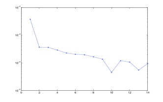
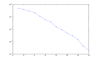
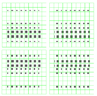
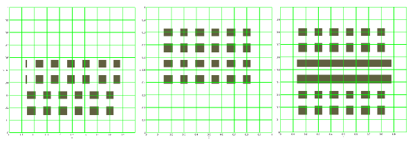
Remark 4 (On norm).
In this remark, we show eigenvalues decay for several choices of and . We consider a target domain within . Our space is generated by solving problems with force terms located outside . We consider several choices for and . First, we choose
where are bilinear basis functions. We also consider
We also consider
where . The last choice is motivated by Babuska and Lipton, 2011, [10]), where a larger domain , (see Figure 4), is used for eigenvalue computations.
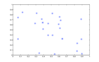
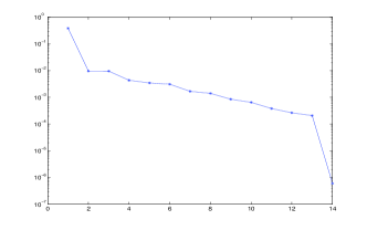
We take to be in and elsewhere. In Figure 3, we plot the eigenvalues corresponding to the above choices of and . The snapshot space is generated using unit force terms in the locations shown in Figure 3, top left. As we see in all the cases the eigenvalues decay fast. The decay of eigenvalues depends on the choices of and , and also on the choice of .
2.3 Step 2. Computing online multiscale basis functions and their coupling
At the online stage, for each parameter value, multiscale basis functions are computed based on each local coarse region. In particular, for each and for each input parameter, we will formulate a quotient for finding a subspace of where the space will be constructed for each (independent of source terms). We seek a subspace of such that for each , there exists such that
| (13) |
for some prescribed error tolerance (different from the one in the offline stage), and the choices of and . The corresponding eigenvalue problem is formed in the space of offline basis functions. We note that, in general, and contain partition of unity functions, penalty terms, and other discretization factors that appear in finite element formulations. In particular, we assume that (where corresponds to (3) in ).
We note that a choice of partition of unity is important to achieve smaller dimensional coarse spaces and one can look for a choice of optimal partition of unity function. Because is a finite dimensional space, the following local eigenvalue problem
| (14) |
can be used to find the basis functions, where and are local matrices corresponding to and , and are corresponding local matrices that are given by
Here, we assume that is a positive definite matrix. Note that the matrices and are computed in the space of offline basis functions. is constructed by selecting eigenvectors corresponding to the largest eigenvalues. In particular, the corresponding eigenvectors are computed by multiplication, in each , where are coordinates of the vector .
More precisely, if we reorder the offline functions using a single index based on the decay of eigenvalues to create the matrices
that are defined on the fine grid, then
where and denote fine scale matrices corresponding to the stiffness and mass matrices at . Under certain requirements for the space , we can guarantee that (10) holds for all (and not only for all which is a smaller subspace).
Once multiscale basis functions are constructed, we project the global solution onto the space of basis functions. One can choose different global coupling methods and we present some of them.
Galerkin coupling. For a Galerkin formulation, we need conforming basis functions. We modify by multiplying the functions from this space with partition of unity functions. The modified space has the same dimension and is given by , where and is supported in . Then, the Galerkin approximation can be written as
If we introduce
| (15) |
then Galerkin formulation is given by
| (16) |
Petrov-Galerkin coupling. We denote and write the PG approximation of the solution as
Then the Petrov-Galerkin formulation is given by
| (17) |
where is defined with (15).
Discontinuous Galerkin coupling
One can also use the discontinuous Galerkin (DG) approach (see also [9, 22, 50]) to couple multiscale basis functions. This may avoid the use of the partition of unity functions; however, a global formulation needs to be chosen carefully. We have been investigating the use of DG coupling and the detailed results will be presented elsewhere. Here, we would like to briefly mention a general global coupling that can be used. The global formulation is given by
| (18) |
where
| (19) |
for all . Each local bilinear form is given as a sum of three bilinear forms:
| (20) |
where is the bilinear form,
| (21) |
where is the restriction of in ; the is the symmetric bilinear form,
where is a weighted average of near the edge , is the length of the edge , and and are two coarse-grid elements sharing the common edge ; and is the penalty bilinear form,
| (22) |
Here is a positive penalty parameter that needs to be selected and its choice affects the performance of GMsFEM. One can choose eigenvalue problems based on DG bilinear forms. We refer to [29] for some results along this direction.
Remark 5 (On the convergence of GMsFEM).
Here, we briefly discuss the convergence of the GMsFEM based on Galerking coupling. We denote the bilinear form (3) on the whole domain by , and by the GMsFEM interpolant, and by an approximation over the patch . Then, the error analysis is the following.
| (23) |
Here, we used the fact that , which is an assumption on the choice of , the inequality (10), and replaced the sum over by the sum over larger regions . We note that the assumption can be easily satisified with an appropriate choice of in continuous Galerkin framework (see [31]). One can choose based on finite element formulation such that . For discontinuous Galerkin formulation (with no partition of unity ), we refer to [29] for the appropriate choice of . The hidden constants depend on the number of neighboring element of each coarse block and the constants in (10) and (13). Moreover, there is an irreducable error . We note that one can obtain sharper estimates using a bootstrap argument in parameter-independent case (see [31, 32]) under some assumptions and show that the error decreases as the coarse-mesh size decreases.
2.4 Iterative solvers - online correction of fine-grid solution
In the previous approach, the coarse spaces are designed to achieve a desired accuracy. One can also iterate (on residual and/or the basis functions) for a given source term and converge to the true solution without increasing the dimension of the coarse space. Both approaches have their application fields and allows computing the fine-grid solution with an increasing accuracy. Next, we briefly describe the solution procedure based on the concept of two-level iterative methods.
We denote by the overlapping decomposition obtained from the original non-overlapping decomposition by enlarging each subdomain to
| (24) |
where dist is some distance function and let be the set of finite element functions with support in and zero trace on the boundary . We also denote by the extension by zero operator.
With the help of , we can correct the coarse-grid solution. A number of approaches can be used. For instance, we write the solution in the form
where are defined in (though it can be taken to be supported in a different domain) and is a partition of unity. Suppose that has zero trace on . We can solve the local problems
with zero boundary condition. Other correction schemes can be implemented to correct the coarse-grid solution. For example, we can use the traces of to correct the solution in each subdomain in a consecutive fashion.
When the bilinear form is symmetric and positive definite, we can consider additive two-level domain decomposition methods to find the solution of the fine-grid finite element problem
| (25) |
where is the fine-grid finite element space of piecewise linear polynomials. The matrix of this linear systems is written as
Here, is the stiffness matrix associated to the bilinear form and such that for all . We can solve the fine-scale linear system iteratively with the preconditioned conjugate gradient (PCG) method (or any other Krylov type method for a non-positive problem). Any other suitable iterative scheme can be used as well. We introduce the two level additive preconditioner of the form
| (26) |
where the local matrices are defined by
| (27) |
The coarse projection matrix is defined by and the online coarse matrix . The columns ’s are fine-grid coordinate vectors corresponding to the basis functions, e.g., in the Galerkin formulations they correspond to the basis functions . See [53, 46] and references therein for more details on various domain decomposition methods.
The application of the preconditioner involves solving local problems in each iteration. In domain decomposition methods, our main goal is to reduce the number of iterations in the iterative procedure. It is well known that a coarse solve needs to be added to the one level preconditioner in order to construct robust methods. The appropriate construction of the coarse space plays a key role in obtaining robust iterative domain decomposition methods. Our methods provide an inexpensive coarse solves and efficient iterative solvers for general parameter-dependent problems. This will be discussed in the next sections.
3 Case studies and relation to existing methods. Discussions and applications
In this section, we illustrate basic concepts via some specific examples. We use existing methods in the literature for multiscale problems and show how these methods can be put under the general framework of the GMsFEM and show some numerical results.
3.1 Case with no parameter
In this section, we write a method proposed in [24] as a special case of GMsFEM. First, we consider a case with no parameter, i.e.,
In this case, offline multiscale basis functions are used for online simulations due to the absence of the parameter. Next, we discuss the construction of multiscale basis functions (see [24, 27, 25]).
The construction of the offline space starts with the snapshot space. We choose the snapshot space as all fine-grid functions within a coarse region.
For the construction of the offline space, we can choose
| (28) |
where is the restriction of in and is the partition of unity corresponding to . For example, for the elliptic equation (see (2)),
As for , we select
The corresponding eigenvalue problem can be explicitly written as before. In our numerical implementation, we choose (see [31] that shows that this is not smaller than (28) in the space of local -harmonic functions).
In the first example, we do not construct an online space and the offline space is used in GMsFEM, . The basis functions are constructed by multiplying the eigenvectors corresponding to the dominant eigenvalues by partition of unity functions, see (15). The Galerkin coupling of these basis functions are performed based on (16). Note that the stiffness is pre-computed in the offline stage and there is no need for any stiffness matrix computation in the online stage.
We point out that the choice of initial partition of unity basis functions , are important in reducing the number of very large eigenvalues. We note that the dimension of the coarse space depends on the choice of and, thus, it is important to have a good choice of . The essential ingredient in designing them is to guarantee that there are fewer large eigenvalues, and thus the coarse space dimension is small. With an initial choice of multiscale basis functions that contain many localizable small-scale features of the solution, one can reduce the dimension of the resulting coarse space.
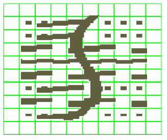
Next, we briefly discuss a few numerical examples (see [24] for more discussions). We present a numerical result for the coarse-scale approximation and for the two-level additive preconditioner (26) with the local spectral multiscale coarse spaces as discussed above. The equation is solved with boundary conditions on . For the coarse-scale approximation, we vary the dimension of the coarse spaces by adding additional basis functions corresponding to the largest eigenvalues. We investigate the convergence rate, while for preconditioning results, we will investigate the behavior of the condition number as we increase the contrast for various choices of coarse spaces. The domain is divided into equal square subdomains. Inside each subdomain we use a fine-scale triangulation, where triangular elements constructed from squares are used. We consider the scalar coefficient depicted in Figure 5 that corresponds to a background one and high conductivity channels and inclusions.
We test the accuracy of GMsFEMs when coarse spaces include eigenvectors corresponding to the large eigenvalues. We implement GMsFEM by choosing the initial partition of unity functions to consist of multiscale functions with linear boundary conditions (MS) (see (29). We use the following notation. GMsFEM refers to the GMsFEM where the coarse space includes all eigenvectors that correspond to eigenvalues which are asymptotically unbounded as the contrast increases, i.e., these eigenvalues increase as we increase the contrast. One of these eigenvectors corresponds to a constant function in the coarse block. GMsFEM refers to the GMsFEM where in addition to eigenvectors that correspond to asymptotically unbounded eigenvalues, we also add eigenvectors corresponding to the next eigenvalues.
In previous studies [36, 37, 31], we discussed how the number of these asymptotically unbounded eigenvalues depends on the number of inclusions and channels. In particular, we showed that if there are inclusions (isolated regions with high conductivity) and channels (isolated high-conductivity regions connecting boundaries of a coarse grid), then the number of asymptotically unbounded eigenvalues is when standard bilinear partition of unity function, , used. However, if the partition of unity is chosen as multiscale finite element basis functions ([40]) defined by
| (29) |
then the number of asymptotically unbounded eigenvalues is . We can also use energy minimizing basis functions that are defined (see [56]) as
| (30) |
subject to with , , to achieve even smaller dimensional coarse spaces.
In all numerical results, the errors are measured in the energy norm (), norm ( ), and -weighted norm () respectively. We present the convergence as we increase the number of additional eigenvectors. In Table 1, we present the numerical results when the initial partition of unity consists of multiscale basis functions with linear boundary conditions for the contrast . We note that the convergence is robust with respect to the contrast and the error reduces. The error is proportional to the largest eigenvalue () whose eigenvector is not included in the coarse space as one can observe from the table (correlation coefficient between and the energy error is ). We observe that the errors are smaller compared to those obtained using MsFEM with piecewise linear initial conditions.
| GMsFEM+0 (153) | 14.3 | 14.3 | 6.17e-02 | 0.0704 |
|---|---|---|---|---|
| GMsFEM+1 (234) | 5.82 | 5.82 | 1.02e-02 | 0.0117 |
| GMsFEM+2 (315) | 5.33 | 5.33 | 8.60e-03 | 0.0071 |
| GMsFEM+3 (396) | 4.64 | 4.64 | 6.53e-03 | 0.0043 |
| GMsFEM+4 (477) | 4.01 | 4.01 | 4.80e-03 | 0.0032 |
Next, we present numerical results when the snapshot space consists of harmonic functions in . More precisely, for each fine-grid function, , which is defined by , where denotes the fine-grid boundary node on , we solve
subject to boundary condition, . We use bilinear partition of unity functions for the mass matrix. The numerical results are presented in Table 2 and we observe slightly worse results compared to Table 1; however, the errors are comparable for dimensions of order . We have observed similar results if larger regions are used for computing snapshot functions (see Remark 4). We report the results on oversampling techniques in [32]
| Coarse dim | ||
|---|---|---|
| dim=202 | 13.7 | 0.2 |
| dim=364 | 3.24 | 1.44e-3 |
| dim=607 | 0.021 | 1.0e-4 |
| dim=850 | 0.164 | 5.6e-5 |
Next, we present the results for a two-level preconditioner. We implement a two-level additive preconditioner with the following coarse spaces: multiscale functions with linear boundary conditions (MS); energy minimizing functions (EMF); spectral coarse spaces using piecewise linear partition of unity functions as an initial space (GMsFEM with Lin); spectral coarse spaces where multiscale finite element basis functions with linear boundary conditions () are used as an initial partition of unity (GMsFEM with MS); spectral coarse spaces with where energy minimizing basis functions () are used as an initial partition of unity (GMsFEM with EMF). In Table 3, we show the number of PCG iterations and estimated condition numbers. We also show the dimensions of the coarse spaces. Note that the standard coarse space with one basis per coarse node has the dimension . The smallest dimension can be achieved by using energy minimizing basis functions as an initial partition of unity. We observe that the number of iterations does not change as the contrast increases when spectral coarse spaces are used. This indicates that the preconditioner is optimal. On the other hand, when using multiscale basis functions (one basis per coarse node), the condition number of the preconditioned matrix increases as the contrast increases.
| MS | EMF | GMsFEM with Lin | GMsFEM with MS | GMsFEM with EMF | |
| 83(2.71e+002) | 69(1.43e+002) | 31(8.60e+000) | 31(9.34e+000) | 32(9.78e+000) | |
| 130(2.65e+004) | 74(1.29e+004) | 33(8.85e+000) | 33(9.72e+000) | 34(1.02e+001) | |
| 189(2.65e+006) | 109(1.29e+006) | 34(8.85e+000) | 35(9.60e+000) | 37(1.02e+001) | |
| Dim | 81 | 81 | 165 | 113 | 113 |
3.2 Elliptic equation with input parameter
Here, we present a method proposed in [30] as a special case of GMsFEM. We consider a parameter-dependent elliptic equation (see (2))
| (31) |
As before, we start the computation with the snapshot space consisting of local fine-grid functions and compute offline basis functions. In this example, we will construct offline multiscale spaces for some selected values of , (), where is the number of selected values of used in constructing multiscale basis functions. These values of are selected via an inexpensive RB procedure [30]. We briefly describe the offline space construction. For each selected (via RB procedure [30]), we choose the offline space
As for , we select
Then, the selected dominant eigenvectors are orthogonalized with respect to inner product.
At the online stage, for each parameter value, multiscale basis functions are computed based on the offline space. In particular, for each and for each input parameter, we formulate a quotient to find a subspace of , where the space will be constructed for each . For the construction of the online space, we choose
For the bilinear form for , we choose
In this case, the online space is a subspace of the offline space and computed by solving an eigenvalue problem for a given value of the parameter . The online space is computed by solving an eigenvalue problem in using , see (14). Using dominant eigenvectors, we form a coarse space as in (15) and solve the global coupled system following (16). For the numerical example, we will consider the coefficient that has an affine representation (see (4)). The online computational cost of assembling the stiffness matrix involves summing pre-computed matrices corresponding to coarse-grid systems. We point out that the choice of initial partition of unity functions, , are important in reducing the number of very large eigenvalues (we refer to [30] for further discussions).
We present a numerical example for which is solved with boundary conditions on . We take that is divided into equal square subdomains. As in Section 3.1, in each subdomain we use a fine-scale triangulation, where triangular elements constructed from squares are used.
We consider a permeability field which is the sum of four permeability fields each of which contains inclusions such that their sum gives several channelized permeability field scenarios. The permeability field is described by
| (32) |
There are several distinct features in this family of conductivity fields which include inclusions and the channels that are obtained by choosing or . There exists no single value of that has all the features. Furthermore, we will use a trial set for the reduced basis algorithm that does not include .
 |
As there are several distinct spatial fields in the space of conductivities, we will choose multiple functions in our reduced basis. In the case of insufficient number of samples in the offline space, we observe that the online permeability field does not contain appropriate features and this affects the convergence rate. We observe in Table 4 that we indeed need to capture all the details of the solution. In this table, we compare the errors obtained by GMsFEM with a different number of online basis functions. We observe convergence with respect to the number of local eigenvectors when increases. We note that in these computations, we also have an error associated with the fact that the offline space is not sufficiently large and thus the error decay is slow as we increase the number of basis functions. We have also computed weighted error which shows a similar trend and the errors are generally much smaller.
| GMsFEM+0 | |||
|---|---|---|---|
| GMsFEM+1 | |||
| GMsFEM+2 | |||
| GMsFEM+3 |
3.3 Anisotropic flows in parameter-dependent media
In this example, we apply GMsFEM to anisotropic flows by considering the elliptic problem with tensor coefficients
where the coefficient is described by
| (33) |
We consider an example from where the first component of the permeability has distinct different features in : inclusions (left), channels (middle), and shifted inclusions (right); see Figure 7. The permeability field is described by
| (34) |
We can represent distinct different features in : inclusions (left), channels (middle), and shifted inclusions (right), see Figure 7. There exists no single value of that has all the features. Furthermore, we will use a trial set for the reduced basis algorithm that does not include .
 |
We will use a trial set for the reduced basis algorithm that does not include . The trial set is chosen as in the case of isotropic case using a greedy algorithm. The important features in these permeability fields characterize the preferred directions of conductivity.
We note that the coarse space has a structure that differs from the case of isotropic coefficients. In particular, the coarse space has a larger dimension and contains all functions that are constant along direction in the examples under consideration [28].
First, we present numerical results for the two-level domain decomposition solvers. In Table 5, we present the results for a two-level preconditioner. We implement a two-level additive preconditioner with the coarse spaces introduced earlier: multiscale functions with linear boundary conditions (MS); spectral coarse spaces where piecewise linear partition of unity functions are used as an initial partition of unity (GMsFEM with Lin); and spectral coarse spaces where multiscale finite element basis functions with linear boundary conditions () are used as an initial partition of unity (GMsFEM with MS).
From this table, we see that the number of PCG iterations and estimated condition numbers do not depend on the contrast when spectral basis functions are used. We use because we need at least three features to represent the permeability field as in the earlier example. We observed from our previous study that if , one could not get a contrast-independent condition number for the preconditioned system. On the other hand, when multiscale basis functions (one basis function per node) is used, the number of iterations and the condition number of the preconditioned system increase as the contrast increases. These results indicate that the preconditioner is optimal when the spectral basis functions are used and the coarse spaces include eigenvectors corresponding to important eigenvalues. Moreover, we observe that the dimension of the coarse space is smaller when multiscale finite element basis functions are used an initial partition of unity.
| MS | GMsFEM with Lin | GMsFEM with MS | |
| Dim | 81 (0.8% of fine DOF) | 862 (8.4% of fine DOF) | 744 (7.4% of fine DOF) |
In Table 6, we present numerical results to study the errors of GMsFEM when the contrast is . As there are three distinct spatial fields in the space of conductivities, we choose at least three realizations. In Table 6, we compare the errors obtained by GMsFEM when the online problem is solved with a corresponding number of basis functions. We observe convergence with respect to the number of local eigenvectors. The convergence with respect to can also be observed.
| GMsFEM+0 | |||
|---|---|---|---|
| GMsFEM+1 | ) | ||
| GMsFEM+2 |
3.4 Some generalizations
The procedure proposed above can be applied to general linear problems such as parabolic and wave equations. The success of the method will depend on the local model reduction that is encoded in , , , and . These bilinear forms need to be appropriately defined for a given .
One can apply GMsFEM to a linearized nonlinear problem where the operator is frozen at the current value of the solution. In this case, one can treat the frozen value of the solution as a scalar parameter on a coarse-grid block level. Note that if global model reduction techniques are used, then one will have to deal with a very large parameter space and these computations will be prohibitively expensive.
To demonstrate this concept, we assume that nonlinear equation is linearized
For example, for the steady-state nonlinear quasilinear equation, we can consider the following linearization (see Section 2.1)
| (35) |
To apply GMsFEM, one can consider as a constant parameter, , within each coarse-grid block. In this case, can be regarded as a parameter that represents the average of the solution in each coarse block (see Section 2.1). In the example of the steady-state Richards’ equation, can be assumed to be a constant within a coarse-grid block. For general problems (e.g., if the linearization is around ), one needs to use higher dimensional parameter space to represent at a coarse-grid level.
The construction of the offline space will follow the GMsFEM procedure (see Section 2.1). We can construct a snapshot space either by taking local fine-grid functions or by using the value of the parameter corresponding to that will appear in the linearization of the global system. Furthermore, the offline space is constructed via a spectral decomposition of the snapshot space as described in Section 2.1.
At the online stage, we consider an approximation of (35) with replaced by its average in each coarse-grid block. We denote this approximate solution by
where is the average of over the coarse regions. For each parameter value , which is the average of the solution on a coarse-grid block , the multiscale basis functions are computed based on the solution of local problem. In particular, for each and for each input parameter and , we formulate a quotient to find a subspace of where the space will be constructed for each . For the construction of the online space, we follow Section 2.1. The online space is computed by solving an eigenvalue problem in using for the current value of see (14). Using dominant eigenvectors, we form a coarse space as in (15) and solve the global coupled system following (16) at the current . For the numerical example, we will consider the coefficient that has an affine representation (see (4)) which reduces the computational cost associated with calculating the stiffness matrix in the online stage (see page Section 3.2).
Remark 6 (Adaptivity in the parameter space).
We note that one can use adaptivity in the parameter space to avoid computing the offline space for a large range of parameters and compute the offline space only for a short range of parameters and update the space. This is, in particular, the case for applications where one has a priori knowledge about how the parameter enters into the problem. To demonstrate this concept, we assume that the parameter space can partitioned into a number of smaller parameter spaces , , where may overlap with each other. Furthermore, the offline spaces are constructed for each . In the online stage, depending on the online value of the parameter, we can decide which offline space to use. This reduces the computational cost in the online stage. In many applications, e.g., in nonlinear problems, one may remain in one of ’s for many iterations and thus use the same offline space to construct the online space.
We present a numerical example for
with on and
| (36) |
where and are defined as in the previous example (see Figure 7). The main objective of this example is to demonstrate that one can use in as a scalar parameter within a coarse-grid block. In contrast, in global methods, if in is used as a parameter, it will be a high dimensional parameter. We will take the average of as a parameter in each coarse-grid block as discussed above.
In Table 7, we present numerical results to study the accuracy of GMsFEM. We take . In our numerical simulations, we use values for the averaged solution in each block and solve local eigenvalue problems for dominant eigenvectors to construct the snapshot space. From this space snapshots in each ), we construct the offline space by selecting the dominant eigenvectors. In Table 7, we present numerical results and show the dimension of the online space at the last iteration. From our numerical results, we observe that the errors are small and decrease as we increase the dimension of the local spectral spaces. The number of iterations needed to converge is the same () for all coarse space dimensions. On the other hand, the error is large if MsFEM with one basis function per node is used. This error in the energy norm is .
| coarse dim | |||
|---|---|---|---|
| 293 | 78.7 | ||
| 352 | 244 | ||
| 620 | 981 |
4 Conclusions
In this paper, we propose a multiscale framework, the Generalized Multiscale Finite Element Method (GMsFEM), for solving PDEs with multiple scales. The main objective is to propose a framework that extends MsFEMs to more general problems with complex input space that includes parameters, high contrast, and right-hand-sides or boundary conditions. The GMsFEM starts with a family of snapshots for the local solutions. These snapshots can usually be generated based on the solutions of local problems or simply taking local fine-grid functions. First, based on the local snapshot space, the offline space is constructed. The construction of the offline space involves solving a spectral problem in the snapshot space. This process introduces a prioritization on the snapshot space across the input space. In the online stage of the simulations, for each new parameter and a source term, the online multiscale basis functions are constructed efficiently. We discuss various constructions. For example, in the absence of parameters, there is no computational work needed in the online stage. When the solution nonlinearly depends on the input space parameters, the construction of the online coarse spaces involves solving a spectral problem over the offline space. We also discuss the online correction of the reduced solution via two-level domain decomposition methods. The optimality of the preconditioners is demonstrated through a few examples. We show that the GMsFEM covers some of existing multiscale methods. The generalization of the GMsFEM to nonlinear problems is also considered. We illustrate these methods through a few numerical examples. Numerical examples suggest that the proposed framework can be effective in studying multiscale problems with an input space dimension and multiple right-hand-sides.
Acknowledgements
We would like to thank Ms. Guanglian Li for helping us with the computations and providing some computational results. Y. Efendiev’s work is partially supported by the DOE and NSF (DMS 0934837 and DMS 0811180). J.Galvis would like to acknowledge partial support from DOE. This publication is based in part on work supported by Award No. KUS-C1-016-04, made by King Abdullah University of Science and Technology (KAUST).
References
- [1] J. E. Aarnes, On the use of a mixed multiscale finite element method for greater flexibility and increased speed or improved accuracy in reservoir simulation, SIAM J. Multiscale Modeling and Simulation, 2 (2004), 421-439.
- [2] J.E. Aarnes and Y. Efendiev, Mixed multiscale finite element for stochastic porous media flows, SIAM Sci. Comp., Volume 30, Issue 5, pp. 2319-2339, 2008. DOI: 10.1137/07070108X.
- [3] J. E. Aarnes, Y. Efendiev, and L. Jiang, Analysis of Multiscale Finite Element Methods using Global Information For Two-Phase Flow Simulations, SIAM MMS, 2008.
- [4] J. E. Aarnes, S. Krogstad, and K.-A. Lie, A hierarchical multiscale method for two-phase flow based upon mixed finite elements and nonuniform grids, Multiscale Model. Simul. 5(2) (2006), pp. 337–363.
- [5] G. Allaire and R. Brizzi, A multiscale finite element method for numerical homogenization, SIAM J. Multiscale Modeling and Simulation, 4(3), 2005, 790-812.
- [6] A.C. Antoulas, Approximation of Large-Scale Dynamical Systems, SIAM Press, Philadelphia, 2005.
- [7] T. Arbogast, Implementation of a locally conservative numerical subgrid upscaling scheme for two-phase Darcy flow, Comput. Geosci., 6 (2002), pp. 453–481.
- [8] T. Arbogast, G. Pencheva, M. F. Wheeler, and I. Yotov, A multiscale mortar mixed finite element method, SIAM J. Multiscale Modeling and Simulation, 6(1), 2007, 319-346.
- [9] D. N. Arnold, F. Brezzi, B. Cockburn, and L. D. Marini, Unified analysis of discontinuous Galerkin methods for elliptic problems, SIAM J. Numer. Anal., 39 (2001/02), pp. 1749–1779 (electronic).
- [10] I. Babuska and R. Lipton, Optimal Local Approximation Spaces for Generalized Finite Element Methods with Application to Multiscale Problems. Multiscale Modeling and Simulation, SIAM 9 (2011) 373-406
- [11] I. Babuška and J. M. Melenk, The partition of unity method, Internat. J. Numer. Methods Engrg., 40 (1997), pp. 727-758.
- [12] I. Babuška and E. Osborn, Generalized Finite Element Methods: Their Performance and Their Relation to Mixed Methods, SIAM J. Numer. Anal., 20 (1983), pp. 510-536.
- [13] M. Barrault, Y. Maday, N.C. Nguyen, and A.T. Patera, An ’Empirical Interpolation’ Method: Application to Efficient Reduced-Basis Discretization of Partial Differential Equations. CR Acad Sci Paris Series I 339:667-672, 2004.
- [14] A. Bensoussan, J.-L. Lions and G. Papanicolaou, Asymptotic Analysis for Periodic Structure, North-Holland, Amsterdam, 1978.
- [15] L. Berlyand and H. Owhadi, Flux norm approach to finite dimensional homogenization approximations with non-separated scales and high contrast, Arch. Ration. Mech. Anal., 198 (2010), pp. 677-721.
- [16] S. Boyoval, Reduced-basis approach for homogenization beyond periodic setting, SIAM MMS, 7(1), 466-494, 2008.
- [17] S. Boyaval, C. LeBris, T. Lelièvre, Y. Maday, N. Nguyen, and A. Patera, Reduced Basis Techniques for Stochastic Problems, Archives of Computational Methods in Engineering, 17:435-454, 2010.
- [18] C.T. Chen, Linear System Theory and Design (2nd. Edition), Holt, Rinehart and Winston, 1984.
- [19] Y. Chen and L. Durlofsky, An ensemble level upscaling approach for efficient estimation of fine-scale production statistics using coarse-scale simulations, SPE paper 106086, presented at the SPE Reservoir Simulation Symposium, Houston, Feb. 26-28 (2007).
- [20] Y. Chen, L.J. Durlofsky, M. Gerritsen, and X.H. Wen, A coupled local-global upscaling approach for simulating flow in highly heterogeneous formations, Advances in Water Resources, 26 (2003), pp. 1041–1060.
- [21] Z. Chen and T.Y. Hou, A mixed multiscale finite element method for elliptic problems with oscillating coefficients, Math. Comp., 72 (2002), 541-576.
- [22] M. Dryja, On discontinuous Galerkin methods for elliptic problems with discontinuous coefficients, Comput. Methods Appl. Math., 3 (2003), pp. 76–85 (electronic).
- [23] L.J. Durlofsky, Numerical calculation of equivalent grid block permeability tensors for heterogeneous porous media, Water Resour. Res., 27 (1991), 699-708.
- [24] Y. Efendiev and J. Galvis, A domain decomposition preconditioner for multiscale high-contrast problems, in Domain Decomposition Methods in Science and Engineering XIX, Huang, Y.; Kornhuber, R.; Widlund, O.; Xu, J. (Eds.), Volume 78 of Lecture Notes in Computational Science and Engineering, Springer-Verlag, 2011, Part 2, 189-196.
- [25] Y. Efendiev and J. Galvis. Coarse-grid multiscale model reduction techniques for flows in heterogeneous media and applications. Chapter of Numerical Analysis of Multiscale Problems, Lecture Notes in Computational Science and Engineering, Vol. 83., pages 97–125.
- [26] Y. Efendiev, J. Galvis and P. Vassielvski, Spectral element agglomerate algebraic multigrid methods for elliptic problems with high-Contrast coefficients, in Domain Decomposition Methods in Science and Engineering XIX, Huang, Y.; Kornhuber, R.; Widlund, O.; Xu, J. (Eds.), Volume 78 of Lecture Notes in Computational Science and Engineering, Springer-Verlag, 2011, Part 3, 407-414.
- [27] Y. Efendiev, J. Galvis, R. Lazarov, and J. Willems, Robust domain decomposition preconditioners for abstract symmetric positive definite bilinear forms, ESAIM: Mathematical Modelling and Numerical Analysis, September 2012, 46, pp. 1175-1199.
- [28] Y. Efendiev, J. Galvis, R. Lazarov, and S. Margenov, J. Ren, Robust two-level domain decomposition preconditioners for high-contrast anisotropic flows in multiscale media, submitted.
- [29] Y. Efendiev, J. Galvis, R. Lazarov, M. Moon, M. Sarkis, Generalized Multiscale Finite Element Method. Symmetric Interior Penalty Coupling, submitted
- [30] Y. Efendiev, J. Galvis, and F. Thomines, A systematic coarse-scale model reduction technique for parameter-dependent flows in highly heterogeneous media and its applications, SIAM MMS 10(4), 1317-1343, 2012.
- [31] Y. Efendiev, J. Galvis, and X. H. Wu, Multiscale finite element methods for high-contrast problems using local spectral basis functions, Journal of Computational Physics. Volume 230, Issue 4, 20 February 2011, Pages 937-955.
- [32] Y. Efendiev, J. Galvis, G. Li, and M. Presho, Generalized Multiscale Finite Element Methods. Oversampling Strategies, Submitted.
- [33] Y. Efendiev, V. Ginting, T. Hou, and R. Ewing, Accurate multiscale finite element methods for two-phase flow simulations, J. Comp. Physics, 220 (1), pp. 155–174, 2006.
- [34] Y. Efendiev and T. Hou, Multiscale finite element methods. Theory and applications, Springer, 2009.
- [35] Y. Efendiev, T. Y. Hou, and X. H. Wu, Convergence of a nonconforming multiscale finite element method, SIAM J. Num. Anal., 37 (2000), 888-910.
- [36] J. Galvis and Y. Efendiev, Domain decomposition preconditioners for multiscale flows in high contrast media, SIAM J. Multiscale Modeling and Simulation, Volume 8, Issue 4, 1461-1483 (2010).
- [37] J. Galvis and Y. Efendiev, Domain decomposition preconditioners for multiscale flows in high-contrast media: Reduced dimension coarse spaces, SIAM J. Multiscale Modeling and Simulation, Volume 8, Issue 5, 1621-1644 (2010).
- [38] I. G. Graham, P. O. Lechner, and R. Scheichl, Domain decomposition for multiscale PDEs, Numer. Math., 106(4):589-626, 2007.
- [39] J. P. Hespanha, Linear systems theory , Princeton University Press, 2009.
- [40] T.Y. Hou and X.H. Wu, A multiscale finite element method for elliptic problems in composite materials and porous media, Journal of Computational Physics, 134 (1997), 169-189.
- [41] T. Hughes, G. Feijoo, L. Mazzei, and J. Quincy, The variational multiscale method - a paradigm for computational mechanics, Comput. Methods Appl. Mech. Engrg, 166 (1998), 3-24.
- [42] P. Jenny, S.H. Lee, and H. Tchelepi, Multi-scale finite volume method for elliptic problems in subsurface flow simulation, J. Comput. Phys., 187 (2003), 47-67.
- [43] S. Krogstad, A Sparse Basis POD for Model Reduction of Multiphase Compressible Flow, SPE 141973. This paper was prepared for presentation at the 2011 SPE Reservoir Simulation Symposium held in The Woodlands, Texas, USA., February 2011.
- [44] I. Lunati and P. Jenny, Multi-scale finite-volume method for compressible multi-phase flow in porous media, J. Comp. Phys., 216:616-636, 2006.
- [45] L. Machiels, Y. Maday, I.B. Oliveira, A.T. Patera, and D.V. Rovas, Output bounds for reduced-basis approximations of symmetric positive definite eigenvalue problems, Comptes Rendus de l’Académie des Sciences, 331(2):153-158, 2000.
- [46] T. P. A. Mathew, Domain decomposition methods for the numerical solution of partial differential equations, volume 61 of Lecture Notes in Computational Science and Engineering, Springer-Verlag, Berlin, 2008.
- [47] N. C. Nguyen, A multiscale reduced-basis method for parameterized elliptic partial differential equations with multiple scales, J. Comp. Physics, 227(23), 9807-9822, 2008.
- [48] H. Owhadi and L. Zhang, Metric based up-scaling, Comm. Pure and Applied Math., vol. LX:675-723, 2007.
- [49] H. Owhadi and L. Zhang, Localized bases for finite dimensional homogenization approximations with non-separated scales and high-contrast, submitted to SIAM MMS, Available at Caltech ACM Tech Report No 2010-04. arXiv:1011.0986.
- [50] Rivière, Béatrice, Discontinuous Galerkin methods for solving elliptic and parabolic equation, vol. 35 of Frontiers in Applied Mathematics, Society for Industrial and Applied Mathematics (SIAM), Philadelphia, 2008.
- [51] G. Rozza, D. B. P Huynh, and A. T. Patera, Reduced basis approximation and a posteriori error estimation for affinely parametrized elliptic coercive partial differential equations. Application to transport and continuum mechanics. Arch Comput Methods Eng 15(3):229?275, 2008.
- [52] M. Sarkis, Nonstandard coarse spaces and Schwarz methods for elliptic problems with discontinuous coefficients using non-conforming elements, Numer. Math., 77(3), 383-406, 1997.
- [53] A. Toselli and O. Widlund. Domain decomposition methods—algorithms and theory, volume 34 of Springer Series in Computational Mathematics, Springer-Verlag, Berlin, 2005.
- [54] S. Volkwein, Proper orthogonal decomposition surrogate models for nonlinear dynamical systems: error estimates and suboptimal control In Reduction of Large-Scale Systems, P. Benner, V. Mehrmann, D. C. Sorensen (eds.), Lecture Notes in Computational Science and Engineering, Vol. 45, 261-306, 2005.
- [55] X.H. Wu, Y. Efendiev, and T.Y. Hou, Analysis of upscaling absolute permeability, Discrete and Continuous Dynamical Systems, Series B, 2 (2002), 185-204.
- [56] J. Xu and L. Zikatanov, On an energy minimizing basis for algebraic multigrid methods, Comput. Visual Sci., 7:121-127, 2004.