Hypergeometric Solutions of the $A_{4}^{(1)}$-Surface $q$-Painlevé IV Equation

Hypergeometric Solutions
of the $\boldsymbol{A_{4}^{(1)}}$-Surface $\boldsymbol{q}$-Painlevé IV Equation

Nobutaka NAKAZONO

N. Nakazono

School of Mathematics and Statistics, The University of Sydney,
New South Wales 2006, Australia nobua.n1222@gmail.com

Received June 06, 2013, in final form August 14, 2014; Published online August 22, 2014

We consider a $q$-Painlevé IV equation which is the $A_{4}^{(1)}$-surface type in the Sakai’s classification. We find three distinct types of classical solutions with determinantal structures whose elements are basic hypergeometric functions. Two of them are expressed by ${}_{2}\varphi_{1}$ basic hypergeometric series and the other is given by ${}_{2}\psi_{2}$ bilateral basic hypergeometric series.

$q$-Painlevé equation; basic hypergeometric function; affine Weyl group; $\tau$-function; projective reduction; orthogonal polynomial

33D05; 33D15; 33D45; 33E17; 39A13

1 Introduction

The focus of this paper is on the following single second-order ordinary difference equation:

$$(X_{n+1}X_{n}-1)(X_{n-1}X_{n}-1)$$

$$\qquad=q^{(-N+2n-m-1)/2}a_{0}a_{1}^{3/2}a_{2}^{2}\frac{\big{(}X_{n}+q^{(N-m)/2}a_{1}^{1/2}\big{)}\big{(}X_{n}+q^{(-N+m)/2}a_{1}^{-1/2}\big{)}}{X_{n}+q^{(-N+n-m)/2}a_{1}^{1/2}a_{2}},$$ (1.1)

where $n\in\mathbb{Z}$ is the independent variable, $X_{n}=X_{n}(m,N)$ is the dependent variable and $m,N\in\mathbb{Z}$ and $a_{0}$, $a_{1}$, $a_{2}$, $q$ $(|q|<1)\in\mathbb{C}^{\ast}$ are parameters. Equation (1.1) is known as a $q$-discrete analog of the Painlevé IV equation ($q$-P_IV) [35].

In 2001, Sakai introduced a geometric approach to the theory of the Painlevé and discrete Painlevé equations (Painlevé systems) and showed the classifications of Painlevé systems by the rational surface [37]. The rational surface can be identified with the space of initial condition, and the group of Cremona isometries associated with the surface generate the affine Weyl group. He also showed that the translation part of the affine Weyl group gives rise to various discrete Painlevé equations. Then, such discrete Painlevé equations are said to have the affine Weyl group symmetries.

In 2004, $q$-P_IV (1.1) was generalized to the following simultaneous first-order ordinary difference equations by the singularity confinement criterion [38]:

$$(y_{k+1}x_{k}-1)(y_{k}x_{k}-1)$$

$$\quad=q^{(-N+4k-m+2l-2)/2}a_{0}a_{1}^{3/2}a_{2}^{2}a_{3}\frac{\big{(}x_{k}+q^{(N-m)/2}a_{1}^{1/2}\big{)}\big{(}x_{k}+q^{(-N+m)/2}a_{1}^{-1/2}\big{)}}{x_{k}+q^{(-N+2k-m+2l)/2}a_{1}^{1/2}a_{2}},$$ (1.2a)

$$(y_{k}x_{k}-1)(y_{k}x_{k-1}-1)$$

$$\quad=q^{(-N+4k-m+2l-4)/2}a_{0}a_{1}^{3/2}a_{2}^{2}a_{3}\frac{\big{(}y_{k}+q^{(N-m)/2}a_{1}^{1/2}\big{)}\big{(}y_{k}+q^{(-N+m)/2}a_{1}^{-1/2}\big{)}}{y_{k}+q^{(-N+2k-m-2)/2}a_{1}^{1/2}a_{2}a_{3}},$$ (1.2b)

where $k\in\mathbb{Z}$ is the independent variable, $x_{k}=x_{k}(l,m,N)$ and $y_{k}=y_{k}(l,m,N)$ are dependent variables and $l,m,N\in\mathbb{Z}$ and $a_{0}$, $a_{1}$, $a_{2}$, $a_{3}$, $q$ $(|q|<1)\in\mathbb{C}^{\ast}$ are parameters. System (1.2) is known as a $q$-discrete analog of the Painlevé V equation ($q$-P_V). It is also known that $q$-P_V (1.2) is the $A_{4}^{(1)}$-surface type in the Sakai’s classification and has the affine Weyl group symmetry of type $A_{4}^{(1)}$.

Conversely, $q$-P_IV (1.1) can be recovered from $q$-P_V (1.2) by putting

$$a_{3}=q^{1/2},\qquad l=0,$$

and replacing the independent variable and the dependent variables by

$$2k=n,\qquad x_{k}=X_{n},\qquad y_{k}=X_{n-1}.$$

This procedure is referred to as “symmetrization” of $q$-P_V (1.2), which comes from the terminology of the Quispel–Roberts–Thompson (QRT) mapping [33, 34]. After this terminology, $q$-P_V (1.2) is sometimes called the “asymmetric discrete Painlevé equation”, and $q$-P_IV (1.1) is called the “symmetric discrete Painlevé equation”. It appears as though the symmetrization is a simple specialization on the level of the equation, but the following problems were known:

1. According to Sakai’s theory [37], the discrete Painlevé equations arise as the birational mappings corresponding to the translations of the affine Weyl groups. The asymmetric discrete Painlevé equations are characterized in this manner, however, it was not known how to characterize the symmetric discrete Painlevé equations as the action of affine Weyl groups;

2. Painlevé systems admit the particular solutions expressible in terms of the hypergeometric type functions (hypergeometric solutions) when some of the parameters take special values (see, for example, [13, 14] and references therein). However, the hypergeometric solutions to the symmetric discrete Painlevé equation cannot be obtained by the naïve specialization of those to the corresponding asymmetric equation.

In [17], the mechanism of the symmetrization was investigated and the nontrivial inconsistency among the hypergeometric solutions were explained in detail by taking an example of $q$-Painlevé equation with the affine Weyl group symmetry of type $(A_{2}+A_{1})^{(1)}$. The key to characterize the symmetric discrete Painlevé equation as the action of affine Weyl group is taking the half-step translation instead of a translation as a time evolution. In general, various discrete dynamical systems of Painlevé type can be obtained from elements of infinite order that are not necessarily translations in the affine Weyl group by taking the projection on appropriate subspaces of the parameter spaces. Such a procedure is called a “projective reduction”.

It is well known that the $\tau$-functions play a crucial role in the theory of integrable systems [25], and it is also possible to introduce them in the theory of Painlevé systems [6, 7, 8, 27, 29, 30, 31, 32]. A representation of the affine Weyl groups can be lifted on the level of the $\tau$-functions [12, 15, 39], which gives rise to various bilinear equations of Hirota type satisfied the $\tau$-functions. Usually, the hypergeometric solutions are derived by reducing the bilinear equations to the Plücker relations by using the contiguity relations satisfied by the entries of determinants [2, 3, 9, 10, 11, 18, 19, 20, 21, 28, 36]. This method is elementary, but it encounters technical difficulties for Painlevé systems with large symmetries. In order to overcome this difficulty, Masuda has proposed a method of constructing hypergeometric solutions under a certain boundary condition on the lattice where the $\tau$-functions live (hypergeometric $\tau$-functions), so that they are consistent with the action of the affine Weyl groups [23, 24, 26]. Although this requires somewhat complex calculations, the merit is that it is systematic and that it can be applied to the systems with large symmetries.

In [16], the list of the simplest hypergeometric solutions to the symmetric $q$-Painlevé equations are shown. In general, hypergeometric solutions of Painlevé systems can be expressed by determinants whose entries are given by hypergeometric type functions. Therefore, it is natural to be curious about the determinant formulae of them. The purpose of this paper is to obtain the determinant formulae of the hypergeometric solutions to the $q$-P_IV via the construction of the hypergeometric $\tau$-functions and the theory of orthogonal polynomials.

This paper is organized as follows: in Section 2, we first introduce a representation of the affine Weyl group of type $A_{4}^{(1)}$. Next, we show how $q$-P_V (1.2) and $q$-P_IV (1.1) can be derived from the representation. In Section 3, we construct the hypergeometric $\tau$-functions for the $q$-P_IV and obtain the hypergeometric solutions of the $q$-P_IV which are expressed by basic hypergeometric series (see Theorems 3.16 and 3.17). In Section 4, we obtain the hypergeometric solutions of the $q$-P_IV which are expressed by bilateral basic hypergeometric series via the theory of orthogonal polynomials (see Theorem 4.3). Some concluding remarks are given in Section 5.

We use the following conventions of $q$-analysis with $|q|,|p|<1$ throughout this paper [1, 22]:

• $q$-shifted factorials:

  $$(a;q)_{\infty}=\prod\limits_{i=1}^{\infty}\big{(}1-aq^{i-1}\big{)},\qquad(a;q)_{\lambda}=\frac{(a;q)_{\infty}}{(aq^{\lambda};q)_{\infty}},$$

  where $\lambda\in\mathbb{C}$;

• Jacobi theta function:

  $$\Theta(a;q)=(a;q)_{\infty}\big{(}qa^{-1};q\big{)}_{\infty};$$

• Elliptic gamma function:

  $$\Gamma(a;p,q)=\frac{\big{(}pqa^{-1};p,q\big{)}_{\infty}}{(a;p,q)_{\infty}},$$

  where

  $$(a;p,q)_{k}=\prod\limits_{i,j=0}^{k-1}\big{(}1-p^{i}q^{j}a\big{)};$$

• Basic hypergeometric series:

  $${}_{s}\varphi_{r}\left(\begin{matrix}a_{1},\dots,a_{s}\\ b_{1},\dots,b_{r}\end{matrix};q,z\right)=\sum\limits_{n=0}^{\infty}\frac{(a_{1},\dots,a_{s};q)_{n}}{(b_{1},\dots,b_{r};q)_{n}(q;q)_{n}}\big{[}(-1)^{n}q^{n(n-1)/2}\big{]}^{1+r-s}z^{n},$$

  where

  $$(a_{1},\dots,a_{s};q)_{n}=\prod\limits_{j=1}^{s}(a_{j};q)_{n};$$

• Bilateral basic hypergeometric series:

  $${}_{s}\psi_{r}\left(\begin{matrix}a_{1},\dots,a_{s}\\ b_{1},\dots,b_{r}\end{matrix};q,z\right)=\sum\limits_{n=-\infty}^{\infty}\frac{(a_{1},\dots,a_{s};q)_{n}}{(b_{1},\dots,b_{r};q)_{n}}\big{[}(-1)^{n}q^{n(n-1)/2}\big{]}^{r-s}z^{n};$$

• Bilateral $q$-integral:

  $$\int^{\infty}_{-\infty}f(t){\rm d}_{q}t=(1-q)\sum\limits_{n=-\infty}^{\infty}\big{(}f(q^{n})+f(-q^{n})\big{)}q^{n}.$$

We note that the following formulae hold:

$$\frac{(a;q)_{\lambda+1}}{(a;q)_{\lambda}}=1-aq^{\lambda},\qquad\frac{\Theta(qa;q)}{\Theta(a;q)}=-a^{-1},\qquad\frac{\Gamma(qa;q,q)}{\Gamma(a;q,q)}=\Theta(a;q).$$

2 Affine Weyl group of type $\boldsymbol{A_{4}^{(1)}}$

2.1 Birational representation of the affine Weyl group of type $\boldsymbol{A_{4}^{(1)}}$

In this section, we formulate the family of Bäcklund transformations of $q$-P_V (1.2) as a birational representation of the affine Weyl group of type $A_{4}^{(1)}$.

Let $s_{i}$ $(i=0,1,2,3,4)$, $\sigma$ and $\iota$ be transformations of the parameters $a_{k}$ $(k=0,1,2,3,4)$ and the variables $f_{j}$ $(j=0,1,2,3,4)$. The action of the transformations on the parameters is given by

$$s_{i}(a_{j})=a_{j}a_{i}^{-a_{ij}},\qquad\sigma(a_{i})=a_{i+1},$$

$$\iota:\ (a_{0},a_{1},a_{2},a_{3},a_{4})\mapsto\big{(}a_{0}^{-1},a_{4}^{-1},a_{3}^{-1},a_{2}^{-1},a_{1}^{-1}\big{)},$$

where $i,j\in\mathbb{Z}/5\mathbb{Z}$ and the symmetric $5\times 5$ matrix

$$A=(a_{ij})_{i,j=0}^{4}=\left(\begin{matrix}2&-1&0&0&-1\\ -1&2&-1&0&0\\ 0&-1&2&-1&0\\ 0&0&-1&2&-1\\ -1&0&0&-1&2\end{matrix}\right)$$

is the Cartan matrix of type $A_{4}^{(1)}$. Moreover, the action on the variables is given by

$$s_{i}(f_{i+2})=\frac{a_{i+3}a_{i+4}(a_{i}a_{i+1}+a_{i+3}f_{i})}{a_{i+1}^{2}f_{i+3}},\qquad s_{i}(f_{i+4})=\frac{a_{i+4}(a_{i+2}+a_{i+4}a_{i}f_{i+1})}{a_{i}a_{i+1}a_{i+2}^{2}f_{i+3}},$$

$$s_{i}(f_{j})=f_{j},\quad j\neq i+2,i+4,\qquad\sigma(f_{i})=f_{i+1},$$

$$\iota:\ (f_{0},f_{1},f_{2},f_{3},f_{4})\mapsto(f_{1},f_{0},f_{4},f_{3},f_{2}),$$

where $i\in\mathbb{Z}/5\mathbb{Z}$. Note that the variables satisfy the following conditions:

$$a_{i+3}^{2}a_{i+4}f_{i}=a_{i+1}(a_{i}a_{i+1}f_{i+2}f_{i+3}-a_{i+3}a_{i+4}),$$

where $i\in\mathbb{Z}/5\mathbb{Z}$. The conditions above look like five, but they are essentially three. Therefore, variables $f_{i}$ are essentially two.

Proposition 2.1 ([2, 37, 39]).

The group of birational transformations $\widetilde{W}\big{(}A_{4}^{(1)}\big{)}=\langle s_{0},s_{1},s_{2},s_{3},$ $s_{4},\sigma,\iota\rangle$ gives a representation of the $($extended$)$ affine Weyl group of type $A_{4}^{(1)}$. Namely, the transformations satisfy the fundamental relations

$$s_{i}^{2}=1,\qquad(s_{i}s_{i\pm 1})^{3}=1,\qquad(s_{i}s_{j})^{2}=1,\quad j\neq i\pm 1,\qquad\sigma^{5}=1,\qquad\sigma s_{i}=s_{i+1}\sigma,$$

$$\iota^{2}=1,\qquad\iota s_{0}=s_{0}\iota,\qquad\iota s_{1}=s_{4}\iota,\qquad\iota s_{2}=s_{3}\iota,$$

where $i,j\in\mathbb{Z}/5\mathbb{Z}$.

In general, for a function $F=F(a_{i},f_{j})$, we let an element $w\in\widetilde{W}\big{(}A_{4}^{(1)}\big{)}$ act as $w.F(a_{i},f_{j})=F(w.a_{i},w.f_{j})$, that is, $w$ acts on the arguments from the left. Note that $q=a_{0}a_{1}a_{2}a_{3}a_{4}$ is invariant under the action of $\langle s_{0},s_{1},s_{2},s_{3},s_{4},\sigma\rangle$. We define the translations $T_{i}$ ($i=0,1,2,3,4$) by

$$T_{0}=\sigma s_{4}s_{3}s_{2}s_{1},\qquad T_{1}=\sigma s_{0}s_{4}s_{3}s_{2},\qquad T_{2}=\sigma s_{1}s_{0}s_{4}s_{3},$$

$$T_{3}=\sigma s_{2}s_{1}s_{0}s_{4},\qquad T_{4}=\sigma s_{3}s_{2}s_{1}s_{0},$$ (2.1)

whose action on the parameters is given by

$$\begin{matrix}T_{0}:\ (a_{0},a_{1},a_{2},a_{3},a_{4})\mapsto\big{(}qa_{0},q^{-1}a_{1},a_{2},a_{3},a_{4}\big{)},\\ T_{1}:\ (a_{0},a_{1},a_{2},a_{3},a_{4})\mapsto\big{(}a_{0},qa_{1},q^{-1}a_{2},a_{3},a_{4}\big{)},\\ T_{2}:\ (a_{0},a_{1},a_{2},a_{3},a_{4})\mapsto\big{(}a_{0},a_{1},qa_{2},q^{-1}a_{3},a_{4}\big{)},\\ T_{3}:\ (a_{0},a_{1},a_{2},a_{3},a_{4})\mapsto\big{(}a_{0},a_{1},a_{2},qa_{3},q^{-1}a_{4}\big{)},\\ T_{4}:\ (a_{0},a_{1},a_{2},a_{3},a_{4})\mapsto\big{(}q^{-1}a_{0},a_{1},a_{2},a_{3},qa_{4}\big{)}.\end{matrix}$$

Note that $T_{i}$ ($i=0,1,2,3,4$) commute with each other and $T_{0}T_{1}T_{2}T_{3}T_{4}=1$.

2.2 Derivations of the $\boldsymbol{q}$-Painlevé equations

In this section, we derive the $q$-Painlevé equations from $\widetilde{W}\big{(}A_{4}^{(1)}\big{)}$. The action of $T_{23}=T_{2}T_{3}$ on $f$-variables can be expressed as

$$(T_{23}(y)x-1)(yx-1)=q^{-1}a_{0}a_{1}^{3/2}a_{2}^{2}a_{3}\frac{\big{(}x+a_{1}^{1/2}\big{)}\big{(}x+a_{1}^{-1/2}\big{)}}{x+a_{1}^{1/2}a_{2}},$$ (2.2)

$$(yx-1)\big{(}yT_{23}^{-1}(x)-1\big{)}=q^{-2}a_{0}a_{1}^{3/2}a_{2}^{2}a_{3}\frac{\big{(}y+a_{1}^{1/2}\big{)}\big{(}y+a_{1}^{-1/2}\big{)}}{y+q^{-1}a_{1}^{1/2}a_{2}a_{3}},$$ (2.3)

where

$$x=a_{0}a_{1}^{1/2}a_{3}^{-1}f_{2},\qquad y=a_{1}^{-1/2}a_{2}^{-1}a_{4}^{-1}s_{4}(f_{1}).$$

Applying $T_{23}^{k}T_{2}^{l}T_{0}^{m}T_{1}^{N}$ on equations (2.2) and (2.3) and putting

$$x_{k}(l,m,N)=T_{23}^{k}T_{2}^{l}T_{0}^{m}T_{1}^{N}(x),\qquad y_{k}(l,m,N)=T_{23}^{k}T_{2}^{l}T_{0}^{m}T_{1}^{N}(y),$$

we obtain $q$-P_V (1.2). Then, we can regard $T_{23}$ and $T_{i}$ ($i=0,1,2,3,4$) as the time evolution and the Bäcklund transformations of $q$-P_V (1.2), respectively. We note that considering the action of $T_{0}$:

$$T_{0}(g)g=\frac{\big{(}f+a_{0}^{-3/4}a_{1}^{1/4}a_{3}^{-1/4}\big{)}\big{(}f+a_{0}^{-3/4}a_{1}^{1/4}a_{3}^{-1/4}a_{4}^{-1}\big{)}}{1+a_{0}^{-1/4}a_{1}^{-1/4}a_{3}^{1/4}f},$$

$$T_{0}^{-1}(f)f=\frac{\big{(}g+a_{0}^{-1/4}a_{1}^{3/4}a_{3}^{1/4}\big{)}\big{(}g+a_{0}^{-1/4}a_{1}^{3/4}a_{2}a_{3}^{1/4}\big{)}}{1+a_{0}^{1/4}a_{1}^{1/4}a_{3}^{-1/4}g},$$

where

$$f=a_{0}^{-3/4}a_{1}^{-3/4}a_{3}^{3/4}f_{0},\qquad g=a_{0}^{3/4}a_{1}^{3/4}a_{3}^{-3/4}f_{2},$$

we obtain another $q$-discrete analog of Painlevé V equation [37]:

$$g_{n{+}1}g_{n}=\frac{\big{(}f_{n}\!+\!q^{{-}n{+}\frac{k{+}l{-}m}{4}}a_{0}^{{-}\frac{3}{4}}a_{1}^{\frac{1}{4}}a_{3}^{{-}\frac{1}{4}}\big{)}\big{(}f_{n}\!+\!q^{{-}n{+}\frac{k{+}l{+}3m}{4}}a_{0}^{{-}\frac{3}{4}}a_{1}^{\frac{1}{4}}a_{3}^{{-}\frac{1}{4}}a_{4}^{{-}1}\big{)}}{1\!+\!q^{\frac{{-}k{-}l{+}m}{4}}a_{0}^{{-}\frac{1}{4}}a_{1}^{{-}\frac{1}{4}}a_{3}^{\frac{1}{4}}f_{n}},$$ (2.4a)

$$f_{n{+}1}f_{n}=\frac{\big{(}g_{n{+}1}\!+\!q^{{-}n{-}1{+}\frac{3k{-}l{+}m}{4}}a_{0}^{{-}\frac{1}{4}}a_{1}^{\frac{3}{4}}a_{3}^{\frac{1}{4}}\big{)}\big{(}g_{n+1}+q^{{-}n{-}1{+}\frac{{-}k{+}3l{+}m}{4}}a_{0}^{{-}\frac{1}{4}}a_{1}^{\frac{3}{4}}a_{2}a_{3}^{\frac{1}{4}}\big{)}}{1\!+\!q^{\frac{k{+}l{-}m}{4}}a_{0}^{\frac{1}{4}}a_{1}^{\frac{1}{4}}a_{3}^{{-}\frac{1}{4}}g_{n+1}},$$ (2.4b)

where

$$f_{n}=f_{n}(k,l,m)=T_{0}^{n}T_{1}^{k}T_{2}^{l}T_{3}^{m}(f),\qquad g_{n}=g_{n}(k,l,m)=T_{0}^{n}T_{1}^{k}T_{2}^{l}T_{3}^{m}(g).$$

Thus, $q$-P_V (1.2) and equation (2.4) are the Bäcklund transformations each other.

In order to derive $q$-P_IV (1.1), we factorize $T_{23}$ as follows

$$T_{23}=R_{23}^{2},$$

where $R_{23}$ is given by

$$R_{23}=\sigma s_{1}s_{0}s_{4}.$$ (2.5)

The action of $R_{23}$ on the parameters is given by

$$R_{23}:\ (a_{0},a_{1},a_{2},a_{3},a_{4})\mapsto\big{(}a_{0},a_{1},a_{2}a_{3},qa_{3}^{-1},q^{-1}a_{3}a_{4}\big{)}.$$

Let us consider the projection of the action of $R_{23}$ on the line

$$a_{3}=q^{1/2}.$$ (2.6)

Then, the action on the parameters becomes translational motion:

$$R_{23}:\ (a_{0},a_{1},a_{2},a_{4})\mapsto\big{(}a_{0},a_{1},q^{1/2}a_{2},q^{-1/2}a_{4}\big{)}.$$

Since the action of $R_{23}$ on the variable $f_{2}$ is given by

$$R_{23}(f_{2})=\frac{q}{a_{0}^{2}a_{1}f_{2}}\left(1+\frac{a_{0}\big{(}a_{0}f_{2}+q^{1/2}\big{)}\big{(}a_{0}a_{1}f_{2}+q^{1/2}\big{)}}{q^{1/2}\big{(}q^{1/2}a_{2}+a_{0}f_{2}\big{)}f_{4}}\right),$$

$$R_{23}^{-1}(f_{2})=\frac{q}{a_{0}^{2}a_{1}f_{2}}\left(1+\frac{a_{1}a_{2}^{2}}{q^{1/2}}f_{4}\right),$$

we obtain

$$\big{(}R_{23}(X)X-1\big{)}\big{(}R_{23}^{-1}(X)X-1\big{)}=q^{-1/2}a_{0}a_{1}^{3/2}a_{2}^{2}\frac{\big{(}X+a_{1}^{1/2}\big{)}\big{(}X+a_{1}^{-1/2}\big{)}}{X+a_{1}^{1/2}a_{2}},$$ (2.7)

where

$$X=q^{-1/2}a_{0}a_{1}^{1/2}f_{2}.$$ (2.8)

Applying $R_{23}^{n}T_{0}^{m}T_{1}^{N}$ on equation (2.7) and putting

$$X_{n}(m,N)=R_{23}^{n}T_{0}^{m}T_{1}^{N}(X),$$

we obtain $q$-P_IV (1.1). Note that $R_{23}$ commute with $T_{i}$ $(i=0,1,4)$ and $T_{0}T_{1}R_{23}^{2}T_{4}=1$. Then, $R_{23}$ and $T_{i}$ $(i=0,1,4)$ are regarded as the time evolution and the Bäcklund transformations of $q$-P_IV (1.1), respectively.

3 Hypergeometric solutions of the $\boldsymbol{q}$-P_IV (I)

In this section, we obtain the hypergeometric solutions of $q$-P_IV (1.1) by constructing the hypergeometric $\tau$-functions for the $q$-P_IV.

3.1 $\boldsymbol{\tau}$-functions

In this section, we define the $\tau$-functions.

We introduce the new variables $\tau_{i}$ $(i=1,2,\dots,7)$ with

$$f_{2}=\frac{\tau_{4}\tau_{5}}{\tau_{6}\tau_{7}},\qquad f_{4}=\frac{\tau_{1}\tau_{2}}{\tau_{3}\tau_{7}},$$ (3.1)

and lift the representation of $\widetilde{W}\big{(}A_{4}^{(1)}\big{)}$ on their level:

$$s_{0}(\tau_{1})=\frac{a_{4}(a_{0}\tau_{3}\tau_{4}\tau_{5}+a_{2}a_{3}\tau_{1}\tau_{2}\tau_{6}+a_{0}a_{3}\tau_{3}\tau_{6}\tau_{7})}{a_{0}^{2}a_{1}a_{2}\tau_{4}\tau_{7}},\qquad s_{0}(\tau_{i})=\tau_{i},\quad i=2,3,5,6,$$

$$s_{0}(\tau_{4})=\frac{a_{0}a_{4}(a_{0}\tau_{3}\tau_{4}\tau_{5}+a_{2}a_{3}\tau_{1}\tau_{2}\tau_{6}+a_{3}\tau_{3}\tau_{6}\tau_{7})}{a_{1}a_{2}\tau_{1}\tau_{7}},$$

$$s_{0}(\tau_{7})=\frac{a_{4}\big{(}a_{0}^{2}\tau_{3}\tau_{4}\tau_{5}+a_{3}a_{0}\tau_{3}\tau_{6}\tau_{7}+a_{2}a_{3}\tau_{1}\tau_{2}\tau_{6}\big{)}}{a_{0}a_{1}a_{2}\tau_{1}\tau_{4}},\qquad s_{1}(\tau_{1})=\tau_{2},\qquad s_{1}(\tau_{2})=\tau_{1},$$

$$s_{1}(\tau_{i})=\tau_{i},\quad i=3,\dots,7,\qquad s_{2}(\tau_{1})=\frac{a_{0}a_{1}(a_{0}\tau_{4}\tau_{5}+a_{2}a_{3}\tau_{6}\tau_{7})}{a_{3}^{2}\tau_{3}},$$

$$s_{2}(\tau_{3})=\frac{a_{0}a_{1}(a_{0}\tau_{4}\tau_{5}+a_{3}\tau_{6}\tau_{7})}{a_{2}a_{3}^{2}\tau_{1}},\qquad s_{2}(\tau_{i})=\tau_{i},\quad i=2,4,5,6,7,$$

$$s_{3}(\tau_{4})=\frac{a_{2}(a_{2}a_{3}\tau_{1}\tau_{2}+a_{0}\tau_{3}\tau_{7})}{a_{0}^{2}a_{3}a_{4}\tau_{6}},\qquad s_{3}(\tau_{6})=\frac{a_{2}a_{3}(a_{2}\tau_{1}\tau_{2}+a_{0}\tau_{3}\tau_{7})}{a_{0}^{2}a_{4}\tau_{4}},$$

$$s_{3}(\tau_{i})=\tau_{i},\quad i=1,2,3,5,7,\qquad s_{4}(\tau_{4})=s_{4}(\tau_{5}),\qquad s_{4}(\tau_{5})=s_{4}(\tau_{4}),$$

$$s_{4}(\tau_{i})=\tau_{i},\quad i=1,2,3,6,7,\qquad\iota:\ (\tau_{1},\tau_{2},\tau_{3},\tau_{4},\tau_{5},\tau_{6},\tau_{7})=(\tau_{4},\tau_{5},\tau_{6},\tau_{1},\tau_{2},\tau_{3},\tau_{7}),$$

$$\sigma(\tau_{1})=\frac{a_{0}a_{1}\left(a_{0}\tau_{4}\tau_{5}+a_{3}\tau_{6}\tau_{7}\right)}{a_{2}a_{3}^{2}\tau_{1}},\qquad\sigma(\tau_{2})=\tau_{3},\qquad\sigma(\tau_{3})=\tau_{6},$$

$$\sigma(\tau_{4})=\frac{a_{4}\big{(}a_{0}^{2}\tau_{3}\tau_{4}\tau_{5}+a_{3}a_{0}\tau_{3}\tau_{6}\tau_{7}+a_{2}a_{3}\tau_{1}\tau_{2}\tau_{6}\big{)}}{a_{0}a_{1}a_{2}\tau_{1}\tau_{4}},\qquad\sigma(\tau_{5})=\tau_{7},$$

$$\sigma(\tau_{6})=\tau_{5},\qquad\sigma(\tau_{7})=\tau_{2}.$$

Then, we get the following proposition:

Proposition 3.1 ([39]).

The transformations: $s_{0}$, $s_{1}$, $s_{2}$, $s_{3}$, $s_{4}$, $\sigma$, $\iota$, on the variables $\tau_{i}$ $(i=1,2,\dots,7)$ also realize the $($extended$)$ affine Weyl group of type $A_{4}^{(1)}$.

Let us define the $\tau$-functions $\tau^{n,m}_{N}$ ($n,m,N\in\mathbb{Z}$) by

$$\tau_{N}^{n,m}=R_{23}^{n}T_{0}^{m}T_{1}^{N}(\tau_{4}).$$

By definition, every $\tau$-function can be determined by a rational function in 7 initial variables $\tau_{i}$ $(i=1,2,\dots,7)$. We note that the 7 initial variables are expressed by the $\tau$-functions as the following (see Fig. 1):

$$\tau_{1}=\tau_{1}^{1,0},\qquad\tau_{2}=\tau_{0}^{1,1},\qquad\tau_{3}=\tau_{1}^{1,1},\qquad\tau_{4}=\tau_{0}^{0,0},$$

$$\tau_{5}=\tau_{1}^{3,1},\qquad\tau_{6}=\tau_{1}^{2,1},\qquad\tau_{7}=\tau_{0}^{1,0}.$$ (3.2)

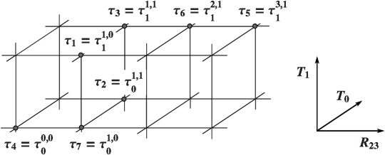
Figure 1: Configuration of the $\tau$-functions on the 3D-lattice.

3.2 Hypergeometric $\boldsymbol{\tau}$-functions for the $\boldsymbol{q}$-P_IV

The aim of this section is to construct the hypergeometric $\tau$-functions for the $q$-P_IV. We define the hypergeometric $\tau$-functions for the $q$-P_IV by $\tau_{N}^{n,m}$ consistent with the action of $\langle R_{23},T_{0}\rangle$. Here, we mean $\tau=\tau(\alpha)$ consistent with an action of transformation $r$ as

$$r.\tau=\tau(r.\alpha).$$

Hereinafter, we impose the condition (2.6), and then regard $\tau$-functions $\tau_{N}^{n,m}$ as the functions in $a_{0}$ and $a_{2}$ consistent with the action of $\langle R_{23},T_{0}\rangle$, i.e.,

$$\tau_{N}^{n,m}=\tau_{N}^{0,0}\big{(}q^{m}a_{0},q^{n/2}a_{2}\big{)}.$$

By definition, every $\tau$-function $\tau_{N}^{n,m}$ is determined by a rational function in $\tau_{0}^{n,m}$ and $\tau_{1}^{n,m}$ (or $\tau_{1},\dots,\tau_{7}$). Thus, our purpose is determining $\tau_{0}^{n,m}$ and $\tau_{1}^{n,m}$ consistent with the action of $\langle R_{23},T_{0}\rangle$ and constructing the closed-form expressions of $\tau_{N}^{n,m}$ $(N\geq 2)$ under the condition

$$a_{0}a_{1}=q,$$ (3.3)

and the boundary condition

$$\tau_{N}^{n,m}=0,\qquad N<0.$$ (3.4)

Henceforth, we construct the hypergeometric $\tau$-functions for the $q$-P_IV in the following four steps.

Step 1. Conditions of $\boldsymbol{\tau_{0}^{n,m}}$

In the first step, we obtain the condition of $\tau_{0}^{n,m}$, which follows from the boundary condition (3.4).

Lemma 3.2.

The following bilinear equations hold:

$$\tau_{N+1}^{n,m}\tau_{N-1}^{n-1,m-1}-q^{(-n-4m+4N+7)/2}a_{0}^{-2}a_{2}^{-1}\tau_{N}^{n,m-1}\tau_{N}^{n-1,m}$$

$$\qquad{}-q^{(-n-2m+4N+4)/2}a_{0}^{-1}a_{2}^{-1}\tau_{N}^{n,m}\tau_{N}^{n-1,m-1}=0,$$ (3.5)

$$\tau_{N+1}^{n,m}\tau_{N-1}^{n-1,m}+q^{2N-n+1}a_{2}^{-2}\big{(}q^{(-n+2N+1)/2}a_{2}^{-1}-1\big{)}\tau_{N}^{n-1,m}\tau_{N}^{n,m}$$

$$\qquad{}-q^{(-3n+6N+3)/2}a_{2}^{-3}\tau_{N}^{n-2,m}\tau_{N}^{n+1,m}=0,$$ (3.6)

$$\tau_{N+1}^{n,m}\tau_{N-1}^{n,m}+q^{(-2n+6N+1)/2}a_{2}^{-2}\big{(}1-q^{N-m+1}a_{0}^{-1}\big{)}\big{(}\tau_{N}^{n,m}\big{)}^{2}$$

$$\qquad{}-q^{4N-4m+4}a_{0}^{-4}\tau_{N}^{n,m-1}\tau_{N}^{n,m+1}=0.$$ (3.7)

Proof 3.3.

Application of $T_{1}$ on $\tau_{3}$ yields the following bilinear equations:

$$T_{1}(\tau_{3})\tau_{4}-q^{2}a_{0}^{-1}a_{1}a_{2}^{-1}\tau_{1}R_{23}^{-1}(\tau_{3})-q^{3/2}a_{1}a_{2}^{-1}\tau_{3}R_{23}^{-1}(\tau_{1})=0,$$ (3.8)

$$T_{1}(\tau_{3})\tau_{2}+q^{3/2}a_{0}a_{1}a_{2}^{-2}(1-a_{1})(\tau_{3})^{2}-a_{1}^{4}\tau_{1}T_{0}(\tau_{3})=0.$$ (3.9)

Applying $R_{23}^{n-1}T_{0}^{m-1}T_{1}^{N-1}$ on equations (3.8) and (3.9) and substituting condition (3.3) in them, we obtain equations (3.5) and (3.7), respectively. Similarly, application of $T_{1}$ on $\tau_{6}$ yields

$$T_{1}(\tau_{6})\tau_{2}+qa_{2}^{-2}\big{(}q^{1/2}a_{2}^{-1}-1\big{)}\tau_{3}\tau_{6}-q^{3/2}a_{2}^{-3}R_{23}^{-1}(\tau_{3})\tau_{5}=0.$$ (3.10)

Then, applying $R_{23}^{n-2}T_{0}^{m-1}T_{1}^{N-1}$ on equation (3.10) and substituting condition (3.3) in it, we obtain equation (3.6). Although we do not write the action of $R_{23}$ and $T_{0}$ on the variables $\tau_{i}$ here, it will be described in the next step.

Putting $N=0$ in equations (3.5)–(3.7) and using the boundary condition (3.4), we get the following conditions:

$$\frac{\tau_{0}^{n+1,m}\tau_{0}^{n,m+1}}{\tau_{0}^{n,m}\tau_{0}^{n+1,m+1}}=-q^{(2m-1)/2}a_{0},$$ (3.11)

$$\frac{\tau_{0}^{n,m}\tau_{0}^{n+3,m}}{\tau_{0}^{n+1,m}\tau_{0}^{n+2,m}}=1-q^{(n+1)/2}a_{2},$$ (3.12)

$$\frac{\tau_{0}^{n,m}\tau_{0}^{n,m+2}}{\big{(}\tau_{0}^{n,m+1}\big{)}^{2}}=q^{(-2n+8m+1)/2}a_{0}^{4}a_{2}^{-2}\big{(}1-q^{-m}a_{0}^{-1}\big{)}.$$ (3.13)

Step 2. Conditions of $\boldsymbol{\tau_{1}^{n,m}}$

In the second step, we shall get the conditions of $\tau_{1}^{n,m}$ from the consistency with the action of $\langle R_{23},T_{0}\rangle$. By definitions (2.1) and (2.5) and Proposition 3.1, the action of $T_{0}$ and $R_{23}$ are given by the follows:

$$T_{0}(\tau_{1})=\tau_{3},\qquad T_{0}(\tau_{7})=\tau_{2},\qquad R_{23}(\tau_{3})=\tau_{6},\qquad R_{23}(\tau_{4})=\tau_{7},\qquad R_{23}(\tau_{6})=\tau_{5},$$

$$T_{0}(\tau_{2})=\frac{q^{3/2}a_{0}a_{1}^{-1}a_{2}^{-1}\tau_{2}T_{0}(\tau_{6})+qa_{0}^{2}a_{2}^{-1}T_{0}(\tau_{4})T_{0}(\tau_{5})}{\tau_{6}},$$ (3.14)

$$T_{0}(\tau_{3})=\frac{a_{0}^{2}a_{1}T_{0}(\tau_{4})T_{0}(\tau_{5})+q^{-1/2}a_{0}a_{1}a_{2}T_{0}(\tau_{6})\tau_{2}}{R_{23}(\tau_{2})},$$ (3.15)

$$T_{0}(\tau_{4})=\frac{a_{2}\tau_{2}\tau_{6}+qa_{0}^{-1}a_{1}^{-2}\tau_{3}R_{23}(\tau_{2})}{\tau_{5}},$$ (3.16)

$$T_{0}(\tau_{5})=\frac{qa_{0}^{-2}a_{1}^{-2}a_{2}^{-1}\tau_{2}\tau_{6}+q^{3/2}a_{0}^{-2}a_{1}^{-3}a_{2}^{-1}\tau_{3}R_{23}(\tau_{2})}{\tau_{4}},$$ (3.17)

$$T_{0}(\tau_{6})=\frac{qa_{1}^{-2}a_{2}^{-1}\tau_{2}\tau_{6}+q^{3/2}a_{0}^{-1}a_{1}^{-3}a_{2}^{-1}\tau_{3}R_{23}(\tau_{2})}{\tau_{7}},$$ (3.18)

$$T_{0}^{-1}(\tau_{1})=\frac{q^{-2}a_{0}^{2}a_{1}a_{2}^{-1}T_{0}^{-1}(\tau_{4})T_{0}^{-1}(\tau_{5})+q^{-1/2}a_{0}a_{1}a_{2}^{-1}T_{0}^{-1}(\tau_{6})T_{0}^{-1}(\tau_{7})}{R_{23}(\tau_{7})},$$ (3.19)

$$T_{0}^{-1}(\tau_{4})=\frac{qa_{0}^{-2}a_{1}^{-2}a_{2}^{-1}\tau_{7}T_{0}^{-1}(\tau_{6})+q^{1/2}a_{0}^{-2}a_{1}^{-3}a_{2}^{-1}\tau_{1}R_{23}(\tau_{7})}{\tau_{5}},$$ (3.20)

$$T_{0}^{-1}(\tau_{5})=\frac{a_{2}\tau_{7}T_{0}^{-1}(\tau_{6})+a_{0}^{-1}a_{1}^{-2}\tau_{1}R_{23}(\tau_{7})}{\tau_{4}},$$ (3.21)

$$T_{0}^{-1}(\tau_{6})=\frac{q^{-1}a_{0}^{2}a_{2}^{-1}\tau_{4}\tau_{5}+q^{-1/2}a_{0}a_{1}^{-1}a_{2}^{-1}\tau_{6}\tau_{7}}{\tau_{2}},$$ (3.22)

$$T_{0}^{-1}(\tau_{7})=\frac{q^{-1}a_{1}^{-2}a_{2}^{-1}\tau_{7}T_{0}^{-1}(\tau_{6})+q^{-1/2}a_{0}^{-1}a_{1}^{-3}a_{2}^{-1}\tau_{1}R_{23}(\tau_{7})}{\tau_{6}},$$ (3.23)

$$R_{23}(\tau_{1})=\frac{q^{-1}a_{0}^{2}a_{2}^{-1}\tau_{4}\tau_{5}+q^{-1/2}a_{0}a_{1}^{-1}a_{2}^{-1}\tau_{6}\tau_{7}}{\tau_{2}},$$ (3.24)

$$R_{23}(\tau_{2})=\frac{q^{-1}a_{0}^{2}a_{1}a_{2}^{-1}\tau_{4}\tau_{5}+q^{-1/2}a_{0}a_{1}a_{2}^{-1}\tau_{6}\tau_{7}}{\tau_{1}},$$ (3.25)

$$R_{23}(\tau_{5})=\frac{q^{3/2}a_{0}^{-2}a_{2}^{2}R_{23}(\tau_{1})R_{23}(\tau_{2})+qa_{0}^{-2}a_{1}^{-1}\tau_{6}R_{23}(\tau_{7})}{\tau_{4}},$$ (3.26)

$$R_{23}(\tau_{7})=\frac{q^{-1}a_{0}^{2}a_{1}\tau_{4}\tau_{5}+q^{-1/2}a_{0}a_{1}a_{2}\tau_{6}\tau_{7}}{\tau_{3}},$$ (3.27)

$$R_{23}^{-1}(\tau_{1})=\frac{q^{-1/2}a_{0}^{2}a_{1}a_{2}^{-1}R_{23}^{-1}(\tau_{4})\tau_{6}+a_{0}a_{1}a_{2}^{-1}\tau_{3}\tau_{4}}{\tau_{2}},$$ (3.28)

$$R_{23}^{-1}(\tau_{2})=\frac{q^{-1/2}a_{0}^{2}a_{2}^{-1}R_{23}^{-1}(\tau_{4})\tau_{6}+a_{0}a_{1}^{-1}a_{2}^{-1}\tau_{3}\tau_{4}}{\tau_{1}},$$ (3.29)

$$R_{23}^{-1}(\tau_{3})=\frac{q^{-1}a_{0}^{2}a_{1}R_{23}^{-1}(\tau_{4})\tau_{6}+q^{-1}a_{0}a_{1}a_{2}\tau_{3}\tau_{4}}{\tau_{7}},$$ (3.30)

$$R_{23}^{-1}(\tau_{4})=\frac{q^{1/2}a_{0}^{-2}a_{2}^{2}\tau_{1}\tau_{2}+qa_{0}^{-2}a_{1}^{-1}\tau_{3}\tau_{7}}{\tau_{5}}.$$ (3.31)

Using notation (3.2) and condition (3.3), we can rewrite equations (3.14)–(3.31) as

$$a_{2}\tau^{2,1}_{1}\tau^{1,2}_{0}=q^{1/2}a_{0}^{2}\tau^{1,1}_{0}\tau^{2,2}_{1}+qa_{0}^{2}\tau^{0,1}_{0}\tau^{3,2}_{1},$$ (3.32)

$$\tau^{2,1}_{0}\tau^{1,2}_{1}=qa_{0}\tau^{0,1}_{0}\tau^{3,2}_{1}+q^{1/2}a_{2}\tau^{2,2}_{1}\tau^{1,1}_{0},$$ (3.33)

$$q\tau^{3,1}_{1}\tau^{0,1}_{0}=qa_{2}\tau^{1,1}_{0}\tau^{2,1}_{1}+a_{0}\tau^{1,1}_{1}\tau^{2,1}_{0},$$ (3.34)

$$q^{3/2}a_{2}\tau^{0,0}_{0}\tau^{3,2}_{1}=q^{1/2}\tau^{1,1}_{0}\tau^{2,1}_{1}+a_{0}\tau^{1,1}_{1}\tau^{2,1}_{0},$$ (3.35)

$$q^{3/2}a_{2}\tau^{1,0}_{0}\tau^{2,2}_{1}=q^{1/2}a_{0}^{2}\tau^{1,1}_{0}\tau^{2,1}_{1}+a_{0}^{2}\tau^{1,1}_{1}\tau^{2,1}_{0},$$ (3.36)

$$a_{2}\tau^{2,0}_{0}\tau^{1,-1}_{1}=q^{-1}a_{0}\tau^{0,-1}_{0}\tau^{3,0}_{1}+q^{1/2}\tau^{2,0}_{1}\tau^{1,-1}_{0},$$ (3.37)

$$q^{5/2}a_{2}\tau^{3,1}_{1}\tau^{0,-1}_{0}=q^{3/2}\tau^{1,0}_{0}\tau^{2,0}_{1}+a_{0}\tau^{1,0}_{1}\tau^{2,0}_{0},$$ (3.38)

$$q^{2}\tau^{0,0}_{0}\tau^{3,0}_{1}=q^{2}a_{2}\tau^{1,0}_{0}\tau^{2,0}_{1}+a_{0}\tau^{1,0}_{1}\tau^{2,0}_{0},$$ (3.39)

$$q^{3/2}a_{2}\tau^{1,1}_{0}\tau^{2,0}_{1}=q^{1/2}a_{0}^{2}\tau^{0,0}_{0}\tau^{3,1}_{1}+a_{0}^{2}\tau^{2,1}_{1}\tau^{1,0}_{0},$$ (3.40)

$$q^{7/2}a_{2}\tau^{2,1}_{1}\tau^{1,-1}_{0}=q^{1/2}a_{0}^{2}\tau^{1,0}_{0}\tau^{2,0}_{1}+a_{0}^{2}\tau^{1,0}_{1}\tau^{2,0}_{0},$$ (3.41)

$$q^{3/2}a_{2}\tau^{1,1}_{0}\tau^{2,0}_{1}=q^{1/2}a_{0}^{2}\tau^{0,0}_{0}\tau^{3,1}_{1}+a_{0}^{2}\tau^{2,1}_{1}\tau^{1,0}_{0},$$ (3.42)

$$a_{2}\tau^{1,0}_{1}\tau^{2,1}_{0}=a_{0}\tau^{0,0}_{0}\tau^{3,1}_{1}+q^{1/2}\tau^{2,1}_{1}\tau^{1,0}_{0},$$ (3.43)

$$a_{0}^{2}\tau^{0,0}_{0}\tau^{4,1}_{1}=q^{3/2}a_{2}^{2}\tau^{2,0}_{1}\tau^{2,1}_{0}+a_{0}\tau^{2,1}_{1}\tau^{2,0}_{0},$$ (3.44)

$$\tau^{1,1}_{1}\tau^{2,0}_{0}=a_{0}\tau^{0,0}_{0}\tau^{3,1}_{1}+q^{1/2}a_{2}\tau^{2,1}_{1}\tau^{1,0}_{0},$$ (3.45)

$$a_{2}\tau^{1,1}_{0}\tau^{0,0}_{1}=q^{1/2}a_{0}\tau^{-1,0}_{0}\tau^{2,1}_{1}+q\tau^{1,1}_{1}\tau^{0,0}_{0},$$ (3.46)

$$qa_{2}\tau^{1,0}_{1}\tau^{0,1}_{0}=q^{1/2}a_{0}^{2}\tau^{-1,0}_{0}\tau^{2,1}_{1}+a_{0}^{2}\tau^{1,1}_{1}\tau^{0,0}_{0},$$ (3.47)

$$\tau^{1,0}_{0}\tau^{0,1}_{1}=a_{0}\tau^{-1,0}_{0}\tau^{2,1}_{1}+a_{2}\tau^{1,1}_{1}\tau^{0,0}_{0},$$ (3.48)

$$a_{0}^{2}\tau^{3,1}_{1}\tau^{-1,0}_{0}=q^{1/2}a_{2}^{2}\tau^{1,0}_{1}\tau^{1,1}_{0}+a_{0}\tau^{1,1}_{1}\tau^{1,0}_{0},$$ (3.49)

respectively. By setting

$$\tau^{n,m}_{1}=\big{(}q^{(n-1)/2}a_{2};q^{1/2}\big{)}_{\infty}\tau^{n,m}_{0}F_{n,m},$$ (3.50)

and using conditions (3.11)–(3.13), equations (3.32)–(3.49) can be reduced to the following contiguity relations:

$$F_{n+2,m}-q^{(n-1)/2}a_{2}F_{n+1,m}-q^{m-2}a_{0}\big{(}1-q^{(n-1)/2}a_{2}\big{)}F_{n,m}=0,$$ (3.51)

$$F_{n+1,m+1}-q^{m-1}a_{0}F_{n,m+1}-q^{(n-2)/2}a_{2}F_{n,m}=0,$$ (3.52)

$$q^{1/2}F_{n+2,m+1}-q^{1/2}F_{n+1,m+1}+q^{(n-1)/2}a_{2}\big{(}1-q^{(n-1)/2}a_{2}\big{)}F_{n,m}=0,$$ (3.53)

$$\big{(}1-q^{m-1}a_{0}\big{)}F_{n+1,m+1}-q^{(n-1)/2}a_{2}F_{n+1,m}-q^{n/2-1}a_{2}\big{(}1-q^{(n-1)/2}a_{2}\big{)}F_{n,m}=0,$$ (3.54)

$$q^{3/2}\big{(}1-q^{m-1}a_{0}\big{)}F_{n+2,m+1}-q^{(n+2)/2}a_{2}F_{n+1,m}$$

$$\qquad{}-q^{(2m+n-1)/2}a_{0}a_{2}\big{(}1-q^{(n-1)/2}a_{2}\big{)}F_{n,m}=0,$$ (3.55)

$$qF_{n+2,m+1}-q^{m}a_{0}F_{n,m+1}-q^{(2n-1)/2}a_{2}^{2}F_{n,m}=0.$$ (3.56)

The correspondence between equations (3.32)–(3.49) and equations (3.51)–(3.56) is established as follows:

$$\eqref{eqn:T0_tau3_2},~{}\eqref{eqn:T0_tau4_2},~{}\eqref{eqn:T0^-1_tau5_2},~{}\eqref{eqn:R23_tau7_2},~{}\eqref{eqn:R23^-1_tau3_2}\Rightarrow\eqref{eqn:relation_F_1},$$

$$\eqref{eqn:T0_tau2_2},~{}\eqref{eqn:T0^-1_tau6_2},~{}\eqref{eqn:R23_tau1_2},~{}\eqref{eqn:R23^-1_tau2_2}\Rightarrow\eqref{eqn:relation_F_2},$$

$$\eqref{eqn:T0^-1_tau1_2},~{}\eqref{eqn:R23_tau2_2},~{}\eqref{eqn:R23^-1_tau1_2}\Rightarrow\eqref{eqn:relation_F_3},$$

$$\eqref{eqn:T0_tau6_2},~{}\eqref{eqn:T0^-1_tau7_2}\Rightarrow\eqref{eqn:relation_F_4},$$

$$\eqref{eqn:T0_tau5_2},~{}\eqref{eqn:T0^-1_tau4_2}\Rightarrow\eqref{eqn:relation_F_5},$$

$$\eqref{eqn:R23_tau5_2},~{}\eqref{eqn:R23^-1_tau4_2}\Rightarrow\eqref{eqn:relation_F_6}.$$

Step 3. Determination of $\boldsymbol{\tau_{0}^{n,m}}$ and $\boldsymbol{\tau_{1}^{n,m}}$

In this step, we determine $\tau_{0}^{n,m}$ and $\tau_{1}^{n,m}$, i.e., we solve equations (3.11)–(3.13) and equations (3.51)–(3.56). It is easily verified that the function

$$\tau_{0}^{n,m}=\big{(}q^{m}a_{0};q,q\big{)}_{\infty}\big{(}q^{(n+1)/2}a_{2};q^{1/2},q\big{)}_{\infty}\Gamma\big{(}q^{(2n+2m-3)/4}a_{0}^{1/2}a_{2};q^{1/2},q^{1/2}\big{)}$$

$$\phantom{\tau_{0}^{n,m}=}{}\times\frac{\Gamma\big{(}q^{(n-m+1)/4}a_{0}^{-1/4}a_{2}^{1/2};q^{1/4},q^{1/4}\big{)}\Gamma\big{(}q^{(n-m)/4}a_{0}^{-1/4}a_{2}^{1/2};q^{1/4},q^{1/4}\big{)}}{\Gamma\big{(}{-}q^{3m-1}a_{0}^{3};q^{3},q^{3}\big{)}\Gamma\big{(}{-}q^{2n}a_{2}^{4};q^{2},q^{2}\big{)}},$$ (3.57)

is the solution of equations (3.11)–(3.13). Therefore, the aim of this step is to solve the equations (3.51)–(3.56). Since equations (3.51)–(3.56) are overdetermined system, let us first consider the essential conditions of $F_{n,m}$.

Lemma 3.4.

Equations (3.51) and (3.52) are essential conditions for $F_{n,m}$.

Proof 3.5.

Eliminating $F_{n,m+1}$ from equations (3.51)_m→m+1 and (3.52), we obtain equation (3.53). In a similar manner, equations (3.54)–(3.56) can be proven by the following procedures: eliminating $F_{n+2,m+1}$ from equations (3.52)_n→n+1 and (3.53), we obtain equation (3.54); eliminating $F_{n+1,m+1}$ from equations (3.52)_n→n+1 and (3.53), we obtain equation (3.55); eliminating $F_{n+1,m+1}$ from equations (3.52) and (3.53), we obtain equation (3.56). These calculations mean that if $F_{n,m}$ satisfies conditions (3.51) and (3.52), then it also satisfies conditions (3.53)–(3.56). Therefore we have completed the proof.

Next, we solve equations (3.51) and (3.52).

Lemma 3.6.

The general solution of contiguity relations (3.51) and (3.52) is given by

$$F_{n,m}=A_{n,m}\frac{\Theta\big{(}q^{n/2}a_{2};q^{1/2}\big{)}\Theta\big{(}q^{(2m-1)/2}a_{0};q\big{)}\big{(}q^{(m-1)/2}a_{0}^{1/2};q^{1/2}\big{)}_{\infty}}{\Theta\big{(}q^{(n+m-2)/2}a_{0}^{1/2}a_{2};q^{1/2}\big{)}}$$

$$\phantom{F_{n,m}=+}{}\times{}_{2}\varphi_{1}\left(\begin{matrix}0,q^{(-m+2)/2}a_{0}^{-1/2}\\ -q^{1/2}\end{matrix};q^{1/2},q^{(n-1)/2}a_{2}\right)$$

$$\phantom{F_{n,m}=}{}+B_{n,m}\frac{\Theta\big{(}q^{n/2}a_{2};q^{1/2}\big{)}\Theta\big{(}q^{(2m-1)/2}a_{0};q\big{)}\big{(}{-}q^{(m-1)/2}a_{0}^{1/2};q^{1/2}\big{)}_{\infty}}{\Theta\big{(}{-}q^{(n+m-2)/2}a_{0}^{1/2}a_{2};q^{1/2}\big{)}}$$

$$\phantom{F_{n,m}=+}\times{}_{2}\varphi_{1}\left(\begin{matrix}0,-q^{(-m+2)/2}a_{0}^{-1/2}\\ -q^{1/2}\end{matrix};q^{1/2},q^{(n-1)/2}a_{2}\right),$$

where $A_{n,m}$ and $B_{n,m}$ are periodic functions of period one for $n$ and $m$, i.e.,

$$A_{n,m}=A_{n+1,m}=A_{n,m+1},\qquad B_{n,m}=B_{n+1,m}=B_{n,m+1}.$$

Proof 3.7.

For convenience, we put

$$t=q^{n/2}a_{2},\qquad\alpha=q^{m}a_{0},\qquad F_{n,m}=F(t,\alpha).$$

Then, equations (3.51) and (3.52) can be rewritten as

$$F(qt,\alpha)-q^{-1/2}tF\big{(}q^{1/2}t,\alpha\big{)}-q^{-2}\alpha\big{(}1-q^{-1/2}t\big{)}F(t,\alpha)=0,$$ (3.58)

$$F\big{(}q^{1/2}t,q\alpha\big{)}-q^{-1}\alpha F(t,q\alpha)-q^{-1}tF(t,\alpha)=0,$$ (3.59)

respectively. Substituting

$$F(t,\alpha)=D(t,\alpha)\sum\limits^{\infty}_{k=0}C_{k}(\alpha)t^{k},$$

in equation (3.58), we obtain

$$D(qt,\alpha)=q^{-2}\alpha D(t,\alpha),$$ (3.60)

$$C_{k}(\alpha)=\frac{\big{(}q^{2}D\big{(}q^{1/2}t,\alpha\big{)}D(t,\alpha)^{-1}\alpha^{-1};q^{1/2}\big{)}_{k}}{q^{k/2}\big{(}{-}q^{1/2},q^{1/2};q^{1/2}\big{)}_{k}}C_{0}(\alpha).$$

Therefore, we obtain the solution of equation (3.58):

$$F(t,\alpha)=D_{1}(t,\alpha)\,{}_{2}\varphi_{1}\left(\begin{matrix}0,q\alpha^{-1/2}\\ -q^{1/2}\end{matrix};q^{1/2},q^{-1/2}t\right)$$

$$\phantom{F(t,\alpha)=}{}+D_{2}(t,\alpha)\,{}_{2}\varphi_{1}\left(\begin{matrix}0,-q\alpha^{-1/2}\\ -q^{1/2}\end{matrix};q^{1/2},q^{-1/2}t\right),$$ (3.61)

where $D_{1}(t,\alpha)$ and $D_{2}(t,\alpha)$ are the solutions of (3.60) which satisfy

$$D_{1}\big{(}q^{1/2}t,\alpha\big{)}=q^{-1}\alpha^{1/2}D_{1}(t,\alpha),$$ (3.62)

$$D_{2}\big{(}q^{1/2}t,\alpha\big{)}=-q^{-1}\alpha^{1/2}D_{2}(t,\alpha),$$ (3.63)

respectively. Substituting (3.61) in equation (3.59), we can obtain the following equations:

$$q^{-1/2}\alpha^{1/2}{}_{2}\varphi_{1}\left(\begin{matrix}0,q^{1/2}\alpha^{-1/2}\\ -q^{1/2}\end{matrix};q^{1/2},t\right)-q^{-1}\alpha\,{}_{2}\varphi_{1}\left(\begin{matrix}0,q^{1/2}\alpha^{-1/2}\\ -q^{1/2}\end{matrix};q^{1/2},q^{-1/2}t\right)$$

$$\qquad{}-q^{-1}t\frac{D_{1}(t,\alpha)}{D_{1}(t,q\alpha)}\,{}_{2}\varphi_{1}\left(\begin{matrix}0,q\alpha^{-1/2}\\ -q^{1/2}\end{matrix};q^{1/2},q^{-1/2}t\right)=0,$$ (3.64)

$$q^{-1/2}\alpha^{1/2}{}_{2}\varphi_{1}\left(\begin{matrix}0,-q^{1/2}\alpha^{-1/2}\\ -q^{1/2}\end{matrix};q^{1/2},t\right)+q^{-1}\alpha\,{}_{2}\varphi_{1}\left(\begin{matrix}0,-q^{1/2}\alpha^{-1/2}\\ -q^{1/2}\end{matrix};q^{1/2},q^{-1/2}t\right)$$

$$\qquad{}+q^{-1}t\frac{D_{2}(t,\alpha)}{D_{2}(t,q\alpha)}\,{}_{2}\varphi_{1}\left(\begin{matrix}0,-q\alpha^{-1/2}\\ -q^{1/2}\end{matrix};q^{1/2},q^{-1/2}t\right)=0.$$ (3.65)

By the definition of basic hypergeometric series ${}_{2}\varphi_{1}$, it is easily verified that

$${}_{2}\varphi_{1}\left(\begin{matrix}0,a\\ c\end{matrix};q^{1/2},z\right)-a^{-1}\,{}_{2}\varphi_{1}\left(\begin{matrix}0,a\\ c\end{matrix};q^{1/2},q^{-1/2}z\right)$$

$$\qquad{}-\big{(}1-a^{-1}\big{)}\,{}_{2}\varphi_{1}\left(\begin{matrix}0,q^{1/2}a\\ c\end{matrix};q^{1/2},q^{-1/2}z\right)=0.$$ (3.66)

Therefore, we obtain the following conditions from equations (3.64) and (3.65) by using equation (3.66):

$$D_{1}(t,q\alpha)=-\frac{t}{\alpha(1-q^{1/2}\alpha^{-1/2})}D_{1}(t,\alpha),$$ (3.67)

$$D_{2}(t,q\alpha)=-\frac{t}{\alpha(1+q^{1/2}\alpha^{-1/2})}D_{2}(t,\alpha).$$ (3.68)

By setting

$$D_{1}(t,\alpha)=\frac{\Theta\big{(}t;q^{1/2}\big{)}\Theta\big{(}q^{-1/2}\alpha;q\big{)}\big{(}q^{-1/2}\alpha^{1/2};q^{1/2}\big{)}_{\infty}}{\Theta\big{(}q^{-1}\alpha^{1/2}t;q^{1/2}\big{)}}A(t,\alpha),$$

$$D_{2}(t,\alpha)=\frac{\Theta\big{(}t;q^{1/2}\big{)}\Theta\big{(}q^{-1/2}\alpha;q\big{)}\big{(}{-}q^{-1/2}\alpha^{1/2};q^{1/2}\big{)}_{\infty}}{\Theta\big{(}{-}q^{-1}\alpha^{1/2}t;q^{1/2}\big{)}}B(t,\alpha),$$

equations (3.62), (3.63), (3.67) and (3.68) can be rewritten as

$$A\big{(}q^{1/2}t,\alpha\big{)}=A(t,\alpha),\qquad B\big{(}q^{1/2}t,\alpha\big{)}=B(t,\alpha),$$

$$A(t,q\alpha)=A(t,\alpha),\qquad B(t,q\alpha)=B(t,\alpha),$$

respectively. This completes the proof.

It was shown that hypergeometric solutions of a symmetric discrete Painlevé equation, which can be obtained by projective reduction, have two expressions and there are the following differences between the two expressions (see [17, Section 2.3]):

1. the bases of hypergeometric series appearing in the solutions are different;

2. the periodicities of periodic functions appearing in the solutions are different.

The differences between these two expressions can be explained by the factorization of the linear difference operators associated with the three-term relation of the hypergeometric functions (see [17, Section 3.2]). Namely, we can see these differences by comparing Lemmas 3.6 and 3.12. To get another expression, we first reselect essential conditions of $F_{n,m}$.

Lemma 3.8.

Equations (3.52) and

$$q^{m-1}a_{0}\big{(}1-q^{m}a_{0}\big{)}F_{n,m+2}-q^{(n-5)/2}a_{2}\big{(}\big{(}1+q^{1/2}\big{)}q^{m}a_{0}-q^{n/2}a_{2}\big{)}F_{n,m+1}$$

$$\qquad{}-q^{(2n-5)/2}a_{2}^{2}F_{n,m}=0,$$ (3.69)

are essential conditions of $F_{n,m}$.

Proof 3.9.

Eliminating $F_{n,m}$ from equations (3.52) and (3.69), we obtain

$$q^{m-2}a_{0}\big{(}1-q^{m-1}a_{0}\big{)}F_{n,m+1}-q^{(n-3)/2}a_{2}F_{n+1,m}$$

$$\qquad{}-q^{(n-5)/2}a_{2}\big{(}q^{(2m-1)/2}a_{0}-q^{n/2}a_{2}\big{)}F_{n,m}=0.$$ (3.70)

Similarly, eliminating $F_{n,m+1}$ from equations (3.52) and (3.70), we obtain

$$\big{(}1-q^{m-1}a_{0}\big{)}F_{n+1,m+1}-q^{(n-1)/2}a_{2}F_{n+1,m}-q^{(n-2)/2}a_{2}\big{(}1-q^{(n-1)/2}a_{2}\big{)}F_{n,m}=0.$$ (3.71)

Finally, eliminating $F_{n+1,m+1}$ from equations (3.70)_n→n+1 and (3.71), we obtain equation (3.51). This result together with Lemma 3.4 complete the proof.

By setting

$$F_{n,m}=\frac{\Theta\big{(}q^{m}a_{0};q\big{)}\Theta\big{(}q^{n/2}a_{2};q^{1/2}\big{)}}{\Theta\big{(}{-}q^{n/2}a_{2};q^{1/2}\big{)}}G_{n-3,m-1},$$ (3.72)

equations (3.52) and (3.69) can be rewritten as

$$q^{-m+1}a_{0}^{-1}G_{n-2,m}+G_{n-3,m}-q^{n/2}a_{2}G_{n-3,m-1}=0,$$ (3.73)

$$G_{n,m-2}+\big{(}q^{-m+1}a_{0}^{-1}-\big{(}1+q^{1/2}\big{)}q^{(-n-3)/2}a_{2}^{-1}\big{)}G_{n,m-1}$$

$$\qquad{}-q^{(-2n-5)/2}a_{2}^{-2}\big{(}q^{-m+1}a_{0}^{-1}-1\big{)}G_{n,m}=0,$$ (3.74)

respectively. Before solving equations (3.73) and (3.74), we prepare the following lemma:

Lemma 3.10.

The following recurrence relations hold:

$${}_{2}\varphi_{1}\left(\begin{matrix}a,b\\ c\end{matrix};q,z\right)-{}_{2}\varphi_{1}\left(\begin{matrix}a,b\\ c\end{matrix};q,qz\right)=\frac{(1-a)(1-b)z}{1-c}\,{}_{2}\varphi_{1}\left(\begin{matrix}qa,qb\\ qc\end{matrix};q,z\right),$$ (3.75)

$$\big{(}q^{-1}c-1\big{)}\,{}_{2}\varphi_{1}\left(\begin{matrix}a,b\\ q^{-1}c\end{matrix};q,z\right)+{}_{2}\varphi_{1}\left(\begin{matrix}a,b\\ c\end{matrix};q,z\right)-q^{-1}c\,{}_{2}\varphi_{1}\left(\begin{matrix}a,b\\ c\end{matrix};q,qz\right)=0.$$ (3.76)

Proof 3.11.

Substituting

$${}_{2}\varphi_{1}\left(\begin{matrix}a,b\\ c\end{matrix};q,z\right)=1+\sum\limits_{n=0}^{\infty}\frac{(qa,qb;q)_{n}}{(qc,q;q)_{n}}\frac{(1-a)(1-b)}{(1-c)\big{(}1-q^{n+1}\big{)}}z^{n+1},$$

in the left-hand side of equation (3.75), we obtain the right-hand side. Equation (3.76) can be easily verified as the following:

$${}_{2}\varphi_{1}\left(\begin{matrix}a,b\\ q^{-1}c\end{matrix};q,z\right)=\sum\limits_{n=0}^{\infty}\frac{(a,b;q)_{n}}{(c,q;q)_{n}}\frac{1-q^{n-1}c}{1-q^{-1}c}z^{n}$$

$$\phantom{{}_{2}\varphi_{1}\left(\begin{matrix}a,b\\ q^{-1}c\end{matrix};q,z\right)}=\frac{1}{1-q^{-1}c}\,{}_{2}\varphi_{1}\left(\begin{matrix}a,b\\ c\end{matrix};q,z\right)-\frac{q^{-1}c}{1-q^{-1}c}\,{}_{2}\varphi_{1}\left(\begin{matrix}a,b\\ c\end{matrix};q,qz\right).$$

Therefore we have completed the proof.

Using Lemma 3.10, we obtain the following lemma:

Lemma 3.12.

The general solution of equations (3.73) and (3.74) is given by

$$G_{n,m}=\Lambda_{n,m}\frac{\Theta\big{(}q^{(n-2m+2)/2}a_{0}^{-1}a_{2};q\big{)}}{\Theta\big{(}q^{-m}a_{0}^{-1};q\big{)}\Theta\big{(}q^{n/2}a_{2};q\big{)}\big{(}q^{(n+3)/2}a_{2};q\big{)}_{\infty}\big{(}q^{-1/2};q\big{)}_{\infty}}$$

$$\phantom{G_{n,m}=+}{}\times{}_{2}\varphi_{1}\left(\begin{matrix}0,q^{(n+3)/2}a_{2}\\ q^{3/2}\end{matrix};q,q^{-m+1}a_{0}^{-1}\right)$$

$$\phantom{G_{n,m}=}{}+\Lambda_{n+1,m}\frac{q^{1/2}\Theta\big{(}q^{(n-2m+3)/2}a_{0}^{-1}a_{2};q\big{)}}{\Theta\big{(}q^{-m}a_{0}^{-1};q\big{)}\Theta\big{(}q^{(n+1)/2}a_{2};q\big{)}\big{(}q^{(n+2)/2}a_{2};q\big{)}_{\infty}\big{(}q^{1/2};q\big{)}_{\infty}}$$

$$\phantom{G_{n,m}=+}\times{}_{2}\varphi_{1}\left(\begin{matrix}0,q^{(n+2)/2}a_{2}\\ q^{1/2}\end{matrix};q,q^{-m+1}a_{0}^{-1}\right),$$

where $\Lambda_{n,m}$ is a periodic function of period two for $n$ and period one for $m$, i.e.,

$$\Lambda_{n+2,m}=\Lambda_{n,m+1}=\Lambda_{n,m}.$$

Proof 3.13.

For convenience, we put

$$t=q^{-m+1}a_{0}^{-1},\qquad\alpha=q^{n/2}a_{2},\qquad G_{n,m}=G(t,\alpha).$$

Then, equations (3.73) and (3.74) can be rewritten as

$$tG\big{(}t,q^{-1}\alpha\big{)}+G\big{(}t,q^{-3/2}\alpha\big{)}-\alpha G\big{(}qt,q^{-3/2}\alpha\big{)}=0,$$ (3.77)

$$G\big{(}q^{2}t,\alpha\big{)}+\big{(}t-\big{(}1+q^{1/2}\big{)}q^{-3/2}\alpha^{-1}\big{)}G(qt,\alpha)-q^{-5/2}\alpha^{-2}(t-1)G(t,\alpha)=0,$$ (3.78)

respectively. Substituting

$$G(t,\alpha)=D(t,\alpha)\sum\limits^{\infty}_{k=0}C_{k}(\alpha)t^{k},$$

in equation (3.78), we obtain

$$G(t,\alpha)=D_{1}(t,\alpha)\,{}_{2}\varphi_{1}\left(\begin{matrix}0,q^{3/2}\alpha\\ q^{3/2}\end{matrix};q,t\right)+D_{2}(t,\alpha)\,{}_{2}\varphi_{1}\left(\begin{matrix}0,q\alpha\\ q^{1/2}\end{matrix};q,t\right),$$ (3.79)

where $D_{1}(t,\alpha)$ and $D_{2}(t,\alpha)$ satisfy

$$D_{1}(qt,\alpha)=q^{-1}\alpha^{-1}D_{1}(t,\alpha),$$ (3.80)

$$D_{2}(qt,\alpha)=q^{-3/2}\alpha^{-1}D_{2}(t,\alpha),$$ (3.81)

respectively. Substituting (3.79) in equation (3.77), we can obtain the following equations:

$${}_{2}\varphi_{1}\left(\begin{matrix}0,q^{-1/2}\alpha\\ q^{1/2}\end{matrix};q,t\right)-{}_{2}\varphi_{1}\left(\begin{matrix}0,q^{-1/2}\alpha\\ q^{1/2}\end{matrix};q,qt\right)=-t\frac{D_{1}\big{(}t,q^{-1}\alpha\big{)}}{D_{2}\big{(}t,q^{-3/2}\alpha\big{)}}\,{}_{2}\varphi_{1}\left(\begin{matrix}0,q^{1/2}\alpha\\ q^{3/2}\end{matrix};q,t\right)\!,\!\!\!\!$$ (3.82)

$$t\frac{D_{2}\big{(}t,q^{-1}\alpha\big{)}}{D_{1}\big{(}t,q^{-3/2}\alpha\big{)}}\,{}_{2}\varphi_{1}\left(\begin{matrix}0,\alpha\\ q^{1/2}\end{matrix};q,t\right)+{}_{2}\varphi_{1}\left(\begin{matrix}0,\alpha\\ q^{3/2}\end{matrix};q,t\right)-q^{1/2}{}_{2}\varphi_{1}\left(\begin{matrix}0,\alpha\\ q^{3/2}\end{matrix};q,qt\right)=0.$$ (3.83)

Therefore, we obtain

$$D_{1}\big{(}t,q^{1/2}\alpha\big{)}=-\frac{1-q\alpha}{1-q^{1/2}}D_{2}(t,\alpha),$$ (3.84)

$$D_{2}\big{(}t,q^{1/2}\alpha\big{)}=-\frac{1-q^{1/2}}{t}D_{1}(t,\alpha),$$ (3.85)

from equations (3.82) and (3.83) by using equations (3.75) and (3.76), respectively. By setting

$$D_{1}(t,\alpha)=\frac{\Theta(\alpha t;q)}{\big{(}q^{-1/2};q\big{)}_{\infty}\big{(}q^{3/2}\alpha;q\big{)}_{\infty}\Theta\big{(}q^{-1}t;q\big{)}\Theta(\alpha;q)}\Lambda(t,\alpha),$$

$$D_{2}(t,\alpha)=\frac{q^{1/2}\Theta(q^{1/2}\alpha t;q)}{\big{(}q^{1/2};q\big{)}_{\infty}(q\alpha;q)_{\infty}\Theta\big{(}q^{-1}t;q\big{)}\Theta\big{(}q^{1/2}\alpha;q\big{)}}\Lambda\big{(}t,q^{1/2}\alpha\big{)},$$

equations (3.80), (3.81), (3.84) and (3.85) can be reduced to

$$\Lambda(t,q\alpha)=\Lambda(qt,\alpha)=\Lambda(t,\alpha).$$

This completes the proof.

Step 4. Constructing the closed-form expressions of $\boldsymbol{\tau_{N}^{n,m}}$ ($\boldsymbol{N\geq 2}$)

In this final step, constructing the closed-form expressions of $\tau_{N}^{n,m}$ $(N\geq 2)$, we obtain the hypergeometric $\tau$-functions for the $q$-P_IV.

Let

$$\tau_{N}^{n,m}=(-1)^{N(N-1)/2}q^{3N(N-1)(N-n+1)/4}a_{2}^{-3N(N-1)/2}\left(\prod\limits_{k=1}^{N}\big{(}q^{(n-2k+1)/2}a_{2};q^{1/2}\big{)}_{\infty}\right)$$

$$\phantom{\tau_{N}^{n,m}=}{}\times\big{(}q^{m}a_{0};q,q\big{)}_{\infty}\big{(}q^{(n+1)/2}a_{2};q^{1/2},q\big{)}_{\infty}\Gamma\big{(}q^{(2n+2m-3)/4}a_{0}^{1/2}a_{2};q^{1/2},q^{1/2}\big{)}$$

$$\phantom{\tau_{N}^{n,m}=}{}\times\frac{\Gamma\big{(}q^{(n-m+1)/4}a_{0}^{-1/4}a_{2}^{1/2};q^{1/4},q^{1/4}\big{)}\Gamma\big{(}q^{(n-m)/4}a_{0}^{-1/4}a_{2}^{1/2};q^{1/4},q^{1/4}\big{)}}{\Gamma\big{(}{-}q^{3m-1}a_{0}^{3};q^{3},q^{3}\big{)}\Gamma\big{(}{-}q^{2n}a_{2}^{4};q^{2},q^{2}\big{)}}\phi_{N}^{n,m}.$$

From (3.4), (3.50) and (3.57), we get

$$\phi_{N}^{n,m}=0,\qquad N<0,\qquad\phi_{0}^{n,m}=1,\qquad\phi_{1}^{n,m}=F_{n,m}.$$

Moreover, it is easily verified that equation (3.6) can be rewritten as

$$\phi_{N+1}^{n,m}\phi_{N-1}^{n-1,m}-\phi_{N}^{n-1,m}\phi_{N}^{n,m}+\phi_{N}^{n-2,m}\phi_{N}^{n+1,m}=0.$$ (3.86)

In general, equation (3.86) admits a solution expressed in terms of Jacobi–Trudi type determinant

$$\phi^{n,m}_{N}=\det(c_{n-2i+j+1,m})_{i,j=1,\ldots,N},\qquad N>0,$$

under the boundary conditions

$$\phi^{n,m}_{N}=0,\qquad N<0,\qquad\phi^{n,m}_{0}=1,\qquad\phi^{n,m}_{1}=c_{n,m},$$

where $c_{n,m}$ is an arbitrary function. Therefore, we obtain the following lemma:

Lemma 3.14.

Under the assumptions

$$a_{0}a_{1}=q,\qquad\tau_{N}^{n,m}=0,\qquad N<0,$$

the hypergeometric $\tau$-functions for the $q$-P_IV are given as

$$\tau_{N}^{n,m}=(-1)^{N(N-1)/2}q^{3N(N-1)(N-n+1)/4}a_{2}^{-3N(N-1)/2}\left(\prod\limits_{k=1}^{N}\big{(}q^{(n-2k+1)/2}a_{2};q^{1/2}\big{)}_{\infty}\right)$$

$$\phantom{\tau_{N}^{n,m}=}{}\times\big{(}q^{m}a_{0};q,q\big{)}_{\infty}\big{(}q^{(n+1)/2}a_{2};q^{1/2},q\big{)}_{\infty}\Gamma\big{(}q^{(2n+2m-3)/4}a_{0}^{1/2}a_{2};q^{1/2},q^{1/2}\big{)}$$

$$\phantom{\tau_{N}^{n,m}=}{}\times\frac{\Gamma\big{(}q^{(n-m+1)/4}a_{0}^{-1/4}a_{2}^{1/2};q^{1/4},q^{1/4}\big{)}\Gamma\big{(}q^{(n-m)/4}a_{0}^{-1/4}a_{2}^{1/2};q^{1/4},q^{1/4}\big{)}}{\Gamma\big{(}{-}q^{3m-1}a_{0}^{3};q^{3},q^{3}\big{)}\Gamma\big{(}{-}q^{2n}a_{2}^{4};q^{2},q^{2}\big{)}}\phi_{N}^{n,m},$$

where

$$\phi_{N}^{n,m}=\begin{vmatrix}F_{n,m}&F_{n+1,m}&\dots&F_{n+N-1,m}\\ F_{n-2,m}&F_{n-1,m}&\dots&F_{n+N-3,m}\\ \vdots&\vdots&\ddots&\vdots\\ F_{n-2N+2,m}&F_{n-2N+3,m}&\dots&F_{n-N+1,m}\end{vmatrix},\quad\phi_{0}^{n,m}=1,\quad\phi_{-N}^{n,m}=0,\quad N>0.$$

Here, $F_{n,m}$ is given in Lemma 3.6.

We also show another expression of the hypergeometric $\tau$-functions for the $q$-P_IV. From relation (3.72), $\phi_{N}^{n,m}$ can be rewritten as

$$\phi_{N}^{n,m}=\Theta\big{(}q^{m}a_{0};q\big{)}^{N}\left(\prod\limits_{k=0}^{N-1}\frac{\Theta\big{(}q^{(n+k)/2}a_{2};q^{1/2}\big{)}}{\Theta\big{(}{-}q^{(n+k)/2}a_{2};q^{1/2}\big{)}}\right)\psi_{N}^{n-3,m-1},$$

where

$$\psi_{N}^{n,m}=\begin{vmatrix}G_{n,m}&G_{n+1,m}&\dots&G_{n+N-1,m}\\ G_{n-2,m}&G_{n-1,m}&\dots&G_{n+N-3,m}\\ \vdots&\vdots&\ddots&\vdots\\ G_{n-2N+2,m}&G_{n-2N+3,m}&\dots&G_{n-N+1,m}\end{vmatrix},\quad\psi_{0}^{n,m}=1,\quad\psi_{-N}^{n,m}=0,\quad N>0.$$

This gives the following lemma:

Lemma 3.15.

Under the assumptions

$$a_{0}a_{1}=q,\qquad\tau_{N}^{n,m}=0,\qquad N<0,$$

the hypergeometric $\tau$-functions for the $q$-P_IV are given as

$$\tau_{N}^{n,m}=(-1)^{N(N-1)/2}q^{3N(N-1)(N-n+1)/4}a_{2}^{-3N(N-1)/2}\left(\prod\limits_{k=1}^{N}\big{(}q^{(n-2k+1)/2}a_{2};q^{1/2}\big{)}_{\infty}\right)$$

$$\phantom{\tau_{N}^{n,m}=}{}\times\big{(}q^{m}a_{0};q,q\big{)}_{\infty}\big{(}q^{(n+1)/2}a_{2};q^{1/2},q\big{)}_{\infty}\Gamma\big{(}q^{(2n+2m-3)/4}a_{0}^{1/2}a_{2};q^{1/2},q^{1/2}\big{)}$$

$$\phantom{\tau_{N}^{n,m}=}{}\times\frac{\Gamma\big{(}q^{(n-m+1)/4}a_{0}^{-1/4}a_{2}^{1/2};q^{1/4},q^{1/4}\big{)}\Gamma\big{(}q^{(n-m)/4}a_{0}^{-1/4}a_{2}^{1/2};q^{1/4},q^{1/4}\big{)}}{\Gamma\big{(}{-}q^{3m-1}a_{0}^{3};q^{3},q^{3}\big{)}\Gamma\big{(}{-}q^{2n}a_{2}^{4};q^{2},q^{2}\big{)}}$$

$$\phantom{\tau_{N}^{n,m}=}{}\times\Theta\big{(}q^{m}a_{0};q\big{)}^{N}\left(\prod\limits_{k=0}^{N-1}\frac{\Theta\big{(}q^{(n+k)/2}a_{2};q^{1/2}\big{)}}{\Theta\big{(}{-}q^{(n+k)/2}a_{2};q^{1/2}\big{)}}\right)\psi_{N}^{n-3,m-1},$$

where

$$\psi_{N}^{n,m}=\begin{vmatrix}G_{n,m}&G_{n+1,m}&\dots&G_{n+N-1,m}\\ G_{n-2,m}&G_{n-1,m}&\dots&G_{n+N-3,m}\\ \vdots&\vdots&\ddots&\vdots\\ G_{n-2N+2,m}&G_{n-2N+3,m}&\dots&G_{n-N+1,m}\end{vmatrix},\quad\psi_{0}^{n,m}=1,\quad\psi_{-N}^{n,m}=0,\quad N>0.$$

Here, $G_{n,m}$ is given in Lemma 3.12.

3.3 Hypergeometric solutions of the $\boldsymbol{q}$-P_IV

In this section, we show the hypergeometric solutions of $q$-P_IV (1.1).

From relations (2.8) and (3.1), the variable for $q$-P_IV (1.1) is expressed by the $\tau$-functions as the following:

$$X_{n}(m,N)=q^{(m+N-1)/2}a_{0}a_{1}^{1/2}\frac{\tau_{N}^{n,m}\tau_{N+1}^{n+3,m+1}}{\tau_{N+1}^{n+2,m+1}\tau_{N}^{n+1,m}}.$$

Therefore, from Lemmas 3.14 and 3.15, we obtain the following theorems:

Theorem 3.16.

The hypergeometric solutions of $q$-P_IV (1.1) with

$$a_{0}a_{1}=q,\qquad N\geq 0,$$ (3.87)

is given by

$$X_{n}(m,N)=-q^{(-2N-m+1)/2}a_{0}^{-1/2}\frac{\phi_{N}^{n,m}\phi_{N+1}^{n+3,m+1}}{\phi_{N+1}^{n+2,m+1}\phi_{N}^{n+1,m}},$$

where

$$\phi_{N}^{n,m}=\begin{vmatrix}F_{n,m}&F_{n+1,m}&\dots&F_{n+N-1,m}\\ F_{n-2,m}&F_{n-1,m}&\dots&F_{n+N-3,m}\\ \vdots&\vdots&\ddots&\vdots\\ F_{n-2N+2,m}&F_{n-2N+3,m}&\dots&F_{n-N+1,m}\end{vmatrix},\qquad\phi_{0}^{n,m}=1.$$

Here, $F_{n,m}$ is given in Lemma 3.6.

Theorem 3.17.

The hypergeometric solutions of $q$-P_IV (1.1) with the condition (3.87) is given by

$$X_{n}(m,N)=q^{(-2N-m+1)/2}a_{0}^{-1/2}\frac{\psi_{N}^{n-3,m-1}\psi_{N+1}^{n,m}}{\psi_{N+1}^{n-1,m}\psi_{N}^{n-2,m-1}},$$

where

$$\psi_{N}^{n,m}=\begin{vmatrix}G_{n,m}&G_{n+1,m}&\dots&G_{n+N-1,m}\\ G_{n-2,m}&G_{n-1,m}&\dots&G_{n+N-3,m}\\ \vdots&\vdots&\ddots&\vdots\\ G_{n-2N+2,m}&G_{n-2N+3,m}&\dots&G_{n-N+1,m}\end{vmatrix},\qquad\psi_{0}^{n,m}=1.$$

Here, $G_{n,m}$ is given in Lemma 3.12.

4 Hypergeometric solutions of the $\boldsymbol{q}$-P_IV (II)

In this section, we show that $q$-P_IV (1.1) also has the hypergeometric solutions expressed by bilateral basic hypergeometric series.

First, we recall the definitions of orthogonal polynomials.

Definition 4.1.

A polynomial sequence $(P_{n}(t))_{n=0}^{\infty}$ which satisfies the following conditions is called an orthogonal polynomial sequence over the field ${\cal K}$, and each term $P_{n}(t)$ is called an orthogonal polynomial over the field ${\cal K}$.

1. deg$(P_{n}(t))=n$;

2. there exists a linear functional ${\cal L}:{\cal K}(t)\to{\cal K}$ which holds the orthogonal condition:

   $${\cal L}[t^{k}P_{n}(t)]=h_{n}\delta_{n,k},\qquad n\geq k,$$

   where $\delta_{n,k}$ is Kronecker’s symbol. Here, $h_{n}$ and $\mu_{n}={\cal L}[t^{n}]$ are called a normalization factor and a moment, respectively.

Definition 4.2.

An orthogonal polynomial sequence whose leading coefficient is $1$ is called a monic orthogonal polynomial sequence (MOPS). Let $(P_{n}(t))_{n=0}^{\infty}$ be a MOPS. Then, polynomial $P_{n}(t)$ and its normalization factor $h_{n}$ are expressed by the moment $\mu_{n}$ as the following:

$$P_{n}=\frac{1}{\Phi_{n}}\begin{vmatrix}\mu_{0}&\mu_{1}&\dots&\mu_{n-1}&\mu_{n}\\ \mu_{1}&\mu_{2}&\dots&\mu_{n}&\mu_{n+1}\\ \vdots&\vdots&\ddots&\vdots&\vdots\\ \mu_{n-1}&\mu_{n}&\dots&\mu_{2n-2}&\mu_{2n-1}\\ 1&t&\dots&t^{n-1}&t^{n}\end{vmatrix},\qquad\!P_{0}=1,\qquad\!h_{n}=\frac{\Phi_{n+1}}{\Phi_{n}},\qquad\!h_{0}=\mu_{0},\!\!\!$$ (4.1)

where $\Phi_{n}$ is the Hankel determinant given by

$$\Phi_{n}=\begin{vmatrix}\mu_{0}&\mu_{1}&\dots&\mu_{n-1}\\ \mu_{1}&\mu_{2}&\dots&\mu_{n}\\ \vdots&\vdots&\ddots&\vdots\\ \mu_{n-1}&\mu_{n}&\dots&\mu_{2n-2}\end{vmatrix}.$$ (4.2)

We assume that $(P_{n})_{n=0}^{\infty}=(P_{n}(t))_{n=0}^{\infty}$ and $(\hat{P}_{n})_{n=0}^{\infty}=(\hat{P}_{n}(t))_{n=0}^{\infty}$ are MOPSs which satisfy the following orthogonal conditions:

$${\cal L}\big{[}t^{k}P_{n}(t)\big{]}=h_{n}\delta_{n,k},\quad n\geq k,\qquad\hat{\cal L}\big{[}t^{k}\hat{P}_{n}(t)\big{]}=\hat{h}_{n}\delta_{n,k},\quad n\geq k,$$

respectively. In addition, we put the case that $P_{n}$ and $\hat{P}_{n}$ are related by the Christoffel transformation (or Geronimus transformation), that is, the linear functionals satisfy the following relation for an arbitrary function $f(t)$:

$${\cal L}[f(t)]=\hat{\cal L}\left[\frac{f(t)}{t-c_{0}}+\delta(t-c_{0})\right],$$

where $\delta(x)$ is the Dirac delta function and $c_{0}\in\mathbb{C}$ is an additional parameter. For these MOPSs, the following relations hold [4, 40, 41]:

$$(t-c_{0})\hat{P}_{n}=P_{n+1}+\frac{\hat{h}_{n}}{h_{n}}P_{n},$$ (4.3)

$$P_{n}=\hat{P}_{n}+\frac{h_{n}}{\hat{h}_{n-1}}\hat{P}_{n-1}.$$ (4.4)

Eliminating $P_{n}$ from equation (4.3) by using equation (4.4), we obtain the following three-term recurrence relation:

$$t\hat{P}_{n}=\hat{P}_{n+1}+\left(\frac{h_{n+1}}{\hat{h}_{n}}+\frac{\hat{h}_{n}}{h_{n}}+c_{0}\right)\hat{P}_{n}+\frac{\hat{h}_{n}}{\hat{h}_{n-1}}\hat{P}_{n-1}.$$ (4.5)

Let

$$\hat{P}_{n}(t)=\frac{\tilde{h}_{n}(c_{1}t;p)}{c_{1}^{n}},\qquad c_{1}>0,$$

where $\tilde{h}_{n}(t;q)$ is the discrete $q$-Hermite II polynomial:

$$\tilde{h}_{n}(t;q)=t^{n}{}_{2}\varphi_{1}\left(\begin{matrix}q^{-n},q^{-n+1}\\ 0\end{matrix};q^{2},-\frac{q^{2}}{t^{2}}\right).$$

Then, the linear functional, the normalization factor and the three-term recurrence relation for $\hat{P}_{n}$ are given by

$$\hat{\cal L}[f(t)]=\int^{\infty}_{-\infty}\frac{f(t)}{\big{(}{-}c_{1}^{2}t^{2};p^{2}\big{)}_{\infty}}{\rm d}_{p}t,$$

$$\hat{h}_{n}=\frac{2}{p^{n^{2}}c_{1}^{2n}}\frac{(p;p)_{n}\big{(}p^{2};p^{2}\big{)}_{\infty}\Theta\big{(}{-}pc_{1}^{2};p^{2}\big{)}}{\big{(}p^{3};p^{2}\big{)}_{\infty}\Theta\big{(}{-}c_{1}^{2};p^{2}\big{)}},$$ (4.6)

$$t\hat{P}_{n}=\hat{P}_{n+1}+p^{-2n+1}\big{(}1-p^{n}\big{)}c_{1}^{-2}\hat{P}_{n-1},$$ (4.7)

respectively. We note that these properties of $q$-Hermite II polynomials are given in [22]. We here impose the condition $c_{0}\neq p^{a}$ for all $a\in\mathbb{Z}$ since the linear functional for $P_{n}$ is given by

$${\cal L}[f(t)]=\int^{\infty}_{-\infty}\frac{f(t)}{(t-c_{0})\big{(}{-}c_{1}^{2}t^{2};p^{2}\big{)}_{\infty}}{\rm d}_{p}t.$$

In addition, the moment $\mu_{n}$ can be obtained by

$$\mu_{n}=-\frac{1-p}{c_{0}^{2}}\sum\limits_{k=-\infty}^{\infty}\frac{\big{(}1-(-1)^{n}\big{)}p^{k}+\big{(}1+(-1)^{n}\big{)}c_{0}}{\big{(}1-p^{2k}c_{0}^{-2}\big{)}\big{(}{-}c_{1}^{2}p^{2k};p^{2}\big{)}_{\infty}}p^{k(n+1)}$$

$$\hphantom{\mu_{n}}{}=\frac{2(1-p)}{\big{(}1-c_{0}^{2}\big{)}\big{(}{-}c_{1}^{2};p^{2}\big{)}_{\infty}}\sum\limits_{k=-\infty}^{\infty}\frac{\big{(}{-}c_{1}^{2},c_{0}^{-2};p^{2}\big{)}_{k}}{\big{(}p^{2}c_{0}^{-2};p^{2}\big{)}_{k}}\left(\frac{1-(-1)^{n}}{2}p^{k}+\frac{1+(-1)^{n}}{2}c_{0}\right)p^{k(n+1)}$$

$$\hphantom{\mu_{n}}{}=\begin{cases}\dfrac{2(1-p)}{\big{(}1-c_{0}^{2}\big{)}\big{(}{-}c_{1}^{2};p^{2}\big{)}_{\infty}}\,{}_{2}\psi_{2}\left(\begin{matrix}-c_{1}^{2},c_{0}^{-2}\\ 0,p^{2}c_{0}^{-2}\end{matrix};p^{2},p^{2k+1}\right),&n=2k-1,\vspace{1mm}\\ \dfrac{2c_{0}(1-p)}{\big{(}1-c_{0}^{2}\big{)}\big{(}{-}c_{1}^{2};p^{2}\big{)}_{\infty}}\,{}_{2}\psi_{2}\left(\begin{matrix}-c_{1}^{2},c_{0}^{-2}\\ 0,p^{2}c_{0}^{-2}\end{matrix};p^{2},p^{2k+1}\right),&n=2k.\end{cases}$$ (4.8)

Comparing the coefficients of equations (4.5) and (4.7), we obtain the following equations:

$$\frac{h_{n+1}}{\hat{h}_{n}}+\frac{\hat{h}_{n}}{h_{n}}+c_{0}=0,$$ (4.9)

$$\frac{\hat{h}_{n}}{\hat{h}_{n-1}}=p^{-2n+1}\big{(}1-p^{n}\big{)}c_{1}^{-2}.$$ (4.10)

From equations (4.9) and (4.10), we obtain

$$\frac{\hat{h}_{n}}{h_{n+1}}=-\frac{h_{n}}{p^{-2n+1}(1-p^{n})c_{1}^{-2}\hat{h}_{n-1}+c_{0}h_{n}}.$$ (4.11)

By setting

$$X_{n}={\rm i}\frac{1-p^{n+1}}{p^{n}c_{1}}\frac{\hat{h}_{n}}{h_{n+1}},$$ (4.12)

equation (4.11) can be rewritten as the following discrete Riccati equation:

$$X_{n}=\frac{1-p^{n+1}}{X_{n-1}+{\rm i}p^{n}c_{1}c_{0}}.$$ (4.13)

Since in the case of

$$a_{0}^{1/2}a_{1}^{1/2}=q^{1/2},\qquad a_{2}=1,\qquad N=-1,$$

$q$-P_IV (1.1) admits the reduction to

$$X_{n}=\frac{1-q^{(n+1)/2}}{X_{n-1}+q^{(n-m+1)/2}a_{0}^{-1/2}},$$

which is equivalent to equation (4.13) with the following correspondence:

$$q^{m/2}a_{0}^{1/2}=-{\rm i}q^{1/2}c_{0}^{-1}c_{1}^{-1},\qquad q^{1/2}=p,$$

(4.1), (4.2), (4.6), (4.8) and (4.12) give the hypergeometric solutions of $q$-P_IV (1.1). Therefore, we finally obtain the following theorem:

Theorem 4.3.

In the case of

$$a_{0}^{1/2}a_{1}^{1/2}=q^{1/2},\qquad a_{2}=1,\qquad N=-1,\qquad n\geq 0,$$

$q$-P_IV (1.1) with

$$q^{m/2}a_{0}^{1/2}=-{\rm i}q^{1/2}c_{0}^{-1}c_{1}^{-1},$$

admits the following hypergeometric solution:

$$X_{n}=\frac{2{\rm i}\big{(}1-q^{(n+1)/2}\big{)}\big{(}q^{1/2};q^{1/2}\big{)}_{n}(q;q)_{\infty}\Theta\big{(}{-}q^{1/2}c_{1}^{2};q\big{)}}{q^{n(n+1)/2}c_{1}^{2n+1}\big{(}q^{3/2};q\big{)}_{\infty}\Theta\big{(}{-}c_{1}^{2};q\big{)}}\frac{\Phi_{n+1}}{\Phi_{n+2}},$$

where

$$\Phi_{n}=\begin{vmatrix}\mu_{0}&\mu_{1}&\dots&\mu_{n-1}\\ \mu_{1}&\mu_{2}&\dots&\mu_{n}\\ \vdots&\vdots&\ddots&\vdots\\ \mu_{n-1}&\mu_{n}&\dots&\mu_{2n-2}\end{vmatrix},$$

$$\mu_{n}=\begin{cases}\dfrac{2\big{(}1-q^{1/2}\big{)}}{\big{(}1-c_{0}^{2}\big{)}\big{(}{-}c_{1}^{2};q\big{)}_{\infty}}\,{}_{2}\psi_{2}\left(\begin{matrix}-c_{1}^{2},c_{0}^{-2}\\ 0,qc_{0}^{-2}\end{matrix};q,q^{(2k+1)/2}\right),&n=2k-1,\vspace{1mm}\\ \dfrac{2c_{0}\big{(}1-q^{1/2}\big{)}}{\big{(}1-c_{0}^{2}\big{)}\big{(}{-}c_{1}^{2};q\big{)}_{\infty}}\,{}_{2}\psi_{2}\left(\begin{matrix}-c_{1}^{2},c_{0}^{-2}\\ 0,qc_{0}^{-2}\end{matrix};q,q^{(2k+1)/2}\right),&n=2k.\end{cases}$$

Here, $c_{0}\neq q^{a/2}$ for all $a\in\mathbb{Z}$.

5 Concluding remarks

In this paper, we have constructed the hypergeometric solutions of $q$-P_IV (1.1) via the construction of the hypergeometric $\tau$-functions and the theory of orthogonal polynomials. We showed that the hypergeometric solutions of the $q$-P_IV can be expressed by the three expressions. We note that the hypergeometric solutions of Painlevé systems expressed by the determinants whose sizes do not depend on the independent variable are called the lattice type solutions, while those expressed by the determinants whose sizes depend on the independent variable are called molecule type solutions. Thus, the hypergeometric solutions given in Theorems 3.16 and 3.17 are lattice type solutions whereas those given in Theorem 4.3 are molecule type solutions.

Before closing, we mention the bilateral type hypergeometric solutions here. It is well known that the coalescence cascade of hypergeometric functions, from the Gauss’s hypergeometric function to the Airy function, corresponds to the diagram of degeneration of the Painlevé equations, from the Painlevé VI equation to the Painlevé II equation, in the sense of the hypergeometric solutions [5]:

$$\begin{matrix}{\rm P}_{\rm VI}&\to&{\rm P}_{\rm V}&\to&{\rm P}_{\rm III}\\ \text{Gauss}&&\text{Kummer}&&\text{Bessel}\\ &&\downarrow&&\downarrow\\ &&{\rm P}_{\rm IV}&\to&{\rm P}_{\rm II}&\\ &&\text{Weber}&&\text{Airy}\end{matrix}$$

Similarly, the relations between basic hypergeometric series and $q$-Painlevé equations are also investigated [14, 16]. However, the hypergeometric solutions described by bilateral basic hypergeometric series have not been considered. It might be an interesting future problem to make a list of the bilateral basic hypergeometric series that appear as the solutions of the $q$-Painlevé equations.

Acknowledgments

The author would like to thank Professors K. Kajiwara, S. Kakei, H. Miki, M. Noumi, and S. Tsujimoto for the useful comments. He also appreciates the valuable comments from the referees which have improved the quality of this paper. This work has been supported by JSPS Grant-in-Aid for Scientific Research No. 22$\cdot$4366 and the Australian Research Council grant DP130100967.

References

- [1] Gasper G., Rahman M., Basic hypergeometric series, Encyclopedia of Mathematics and its Applications, Vol. 96, 2nd ed., Cambridge University Press, Cambridge, 2004.
- [2] Hamamoto T., Kajiwara K., Hypergeometric solutions to the -Painlevé equation of type , J. Phys. A: Math. Gen. 40 (2007), 12509–12524, nlin.SI/0701001.
- [3] Hamamoto T., Kajiwara K., Witte N.S., Hypergeometric solutions to the -Painlevé equation of type , Int. Math. Res. Not. 2006 (2006), 84619, 26 pages, nlin.SI/0607065.
- [4] Ismail M.E.H., Classical and quantum orthogonal polynomials in one variable, Encyclopedia of Mathematics and its Applications, Vol. 98, Cambridge University Press, Cambridge, 2005.
- [5] Iwasaki K., Kimura H., Shimomura S., Yoshida M., From Gauss to Painlevé. A modern theory of special functions, Aspects of Mathematics, Vol. E16, Friedr. Vieweg & Sohn, Braunschweig, 1991.
- [6] Jimbo M., Miwa T., Monodromy preserving deformation of linear ordinary differential equations with rational coefficients. II, Phys. D 2 (1981), 407–448.
- [7] Jimbo M., Miwa T., Monodromy preserving deformation of linear ordinary differential equations with rational coefficients. III, Phys. D 4 (1981), 26–46.
- [8] Jimbo M., Miwa T., Ueno K., Monodromy preserving deformation of linear ordinary differential equations with rational coefficients. I. General theory and -function, Phys. D 2 (1981), 306–352.
- [9] Joshi N., Kajiwara K., Mazzocco M., Generating function associated with the Hankel determinant formula for the solutions of the Painlevé IV equation, Funkcial. Ekvac. 49 (2006), 451–468, nlin.SI/0512041.
- [10] Kajiwara K., Kimura K., On a -difference Painlevé III equation. I. Derivation, symmetry and Riccati type solutions, J. Nonlinear Math. Phys. 10 (2003), 86–102, nlin.SI/0205019.
- [11] Kajiwara K., Masuda T., A generalization of determinant formulae for the solutions of Painlevé II and XXXIV equations, J. Phys. A: Math. Gen. 32 (1999), 3763–3778, solv-int/9903014.
- [12] Kajiwara K., Masuda T., Noumi M., Ohta Y., Yamada Y., solution to the elliptic Painlevé equation, J. Phys. A: Math. Gen. 36 (2003), L263–L272, nlin.SI/0303032.
- [13] Kajiwara K., Masuda T., Noumi M., Ohta Y., Yamada Y., Hypergeometric solutions to the -Painlevé equations, Int. Math. Res. Not. 2004 (2004), 2497–2521, nlin.SI/0403036.
- [14] Kajiwara K., Masuda T., Noumi M., Ohta Y., Yamada Y., Construction of hypergeometric solutions to the -Painlevé equations, Int. Math. Res. Not. 2005 (2005), 1441–1463, nlin.SI/0501051.
- [15] Kajiwara K., Masuda T., Noumi M., Ohta Y., Yamada Y., Point configurations, Cremona transformations and the elliptic difference Painlevé equation, in Théories asymptotiques et équations de Painlevé, Sémin. Congr., Vol. 14, Soc. Math. France, Paris, 2006, 169–198, nlin.SI/0411003.
- [16] Kajiwara K., Nakazono N., Hypergeometric solutions to the symmetric -Painlevé equations, Int. Math. Res. Not., to appear, arXiv:1304.0858.
- [17] Kajiwara K., Nakazono N., Tsuda T., Projective reduction of the discrete Painlevé system of type , Int. Math. Res. Not. (2011), 930–966, arXiv:0910.4439.
- [18] Kajiwara K., Noumi M., Yamada Y., A study on the fourth -Painlevé equation, J. Phys. A: Math. Gen. 34 (2001), 8563–8581, nlin.SI/0012063.
- [19] Kajiwara K., Ohta Y., Determinant structure of the rational solutions for the Painlevé IV equation, J. Phys. A: Math. Gen. 31 (1998), 2431–2446, solv-int/9709011.
- [20] Kajiwara K., Ohta Y., Satsuma J., Casorati determinant solutions for the discrete Painlevé III equation, J. Math. Phys. 36 (1995), 4162–4174, solv-int/9412004.
- [21] Kajiwara K., Ohta Y., Satsuma J., Grammaticos B., Ramani A., Casorati determinant solutions for the discrete Painlevé-II equation, J. Phys. A: Math. Gen. 27 (1994), 915–922, solv-int/9310002.
- [22] Koekoek R., Lesky P.A., Swarttouw R.F., Hypergeometric orthogonal polynomials and their -analogues, Springer Monographs in Mathematics, Springer-Verlag, Berlin, 2010.
- [23] Masuda T., Hypergeometric -functions of the -Painlevé system of type , SIGMA 5 (2009), 035, 30 pages, arXiv:0903.4102.
- [24] Masuda T., Hypergeometric -functions of the -Painlevé system of type , Ramanujan J. 24 (2011), 1–31.
- [25] Miwa T., Jimbo M., Date E., Solitons. Differential equations, symmetries and infinite-dimensional algebras, Cambridge Tracts in Mathematics, Vol. 135, Cambridge University Press, Cambridge, 2000.
- [26] Nakazono N., Hypergeometric functions of the -Painlevé systems of type , SIGMA 6 (2010), 084, 16 pages, arXiv:1008.2595.
- [27] Noumi M., Painlevé equations through symmetry, Translations of Mathematical Monographs, Vol. 223, Amer. Math. Soc., Providence, RI, 2004.
- [28] Ohta Y., Nakamura A., Similarity KP equation and various different representations of its solutions, J. Phys. Soc. Japan 61 (1992), 4295–4313.
- [29] Okamoto K., Studies on the Painlevé equations. III. Second and fourth Painlevé equations, and , Math. Ann. 275 (1986), 221–255.
- [30] Okamoto K., Studies on the Painlevé equations. I. Sixth Painlevé equation , Ann. Mat. Pura Appl. 146 (1987), 337–381.
- [31] Okamoto K., Studies on the Painlevé equations. II. Fifth Painlevé equation , Japan. J. Math. (N.S.) 13 (1987), 47–76.
- [32] Okamoto K., Studies on the Painlevé equations. IV. Third Painlevé equation , Funkcial. Ekvac. 30 (1987), 305–332.
- [33] Quispel G.R.W., Roberts J.A.G., Thompson C.J., Integrable mappings and soliton equations, Phys. Lett. A 126 (1988), 419–421.
- [34] Quispel G.R.W., Roberts J.A.G., Thompson C.J., Integrable mappings and soliton equations. II, Phys. D 34 (1989), 183–192.
- [35] Ramani A., Grammaticos B., Discrete Painlevé equations: coalescences, limits and degeneracies, Phys. A 228 (1996), 160–171, solv-int/9510011.
- [36] Sakai H., Casorati determinant solutions for the -difference sixth Painlevé equation, Nonlinearity 11 (1998), 823–833.
- [37] Sakai H., Rational surfaces associated with affine root systems and geometry of the Painlevé equations, Comm. Math. Phys. 220 (2001), 165–229.
- [38] Tamizhmani K.M., Grammaticos B., Carstea A.S., Ramani A., The -discrete Painlevé IV equations and their properties, Regul. Chaotic Dyn. 9 (2004), 13–20.
- [39] Tsuda T., Tau functions of -Painlevé III and IV equations, Lett. Math. Phys. 75 (2006), 39–47.
- [40] Uvarov V.B., The connection between systems of polynomials that are orthogonal with respect to different distribution functions, USSR Comput. Math. Math. Phys. 9 (1969), no. 6, 25–36.
- [41] Zhedanov A., Rational spectral transformations and orthogonal polynomials, J. Comput. Appl. Math. 85 (1997), 67–86.