Dynamical functional prediction and classification, with application to traffic flow prediction

Abstract

Motivated by the need for accurate traffic flow prediction in transportation management, we propose a functional data method to analyze traffic flow patterns and predict future traffic flow. In this study we approach the problem by sampling traffic flow trajectories from a mixture of stochastic processes. The proposed functional mixture prediction approach combines functional prediction with probabilistic functional classification to take distinct traffic flow patterns into account. The probabilistic classification procedure, which incorporates functional clustering and discrimination, hinges on subspace projection. The proposed methods not only assist in predicting traffic flow trajectories, but also identify distinct patterns in daily traffic flow of typical temporal trends and variabilities. The proposed methodology is widely applicable in analysis and prediction of longitudinally recorded functional data.

T1Supported by Grants 99-ASIS-02 from Academia Sinica and NSC101-2118-M-001-011-MY3 from National Science Council, Taiwan.

1 Introduction

Traffic flow is an important macroscopic traffic characteristic in transportation systems. The measurement and forecasting of traffic flow are crucial in the design, planning and operations of highway facilities [Zhang and Ye (2008)]. Traffic flow can be measured automatically using various types of vehicle detectors such as the commonly used dual loop detectors, which are installed in certain roads at regular intervals. Real-time traffic flow information in conjunction with historical traffic flow records makes it possible to predict traffic flow in the short term. The importance of traffic prediction for intelligent transportation systems has long been recognized in many applications, including the development of traffic control strategies in advanced traffic management systems and real-time route guidance in advanced traveler information systems [Zheng, Lee and Shi (2006)]. However, dynamic features of traffic flow, along with unstable traffic conditions and unpredictable environmental factors, contribute to the challenge of pursuing accuracy in predictions.

Short-term traffic flow prediction has been intensively investigated for more than two decades and various types of methodologies have been developed. These include time series models [e.g., Williams and Hoel (2003), Stathopoulos and Karlaftis (2003)], Kalman filtering methods [e.g., Xie, Zhang and Ye (2007), Okutani and Stephanides (1984)], local linear regression models [Sun et al. (2003)], neural network based methods [e.g., Chen and Grant-Muller (2001), Zheng, Lee and Shi (2006), Çetiner, Sari and Borat (2010)] and fuzzy neural models and fuzzy logic system methods [Yin et al. (2002), Zhang and Ye (2008)], among others. In addition, there are many articles comparing parametric time series models, nonparametric regression models and neural networks in traffic prediction, such as in Kirby, Waston and Dougherty (1997), Smith and Demetsky (1997) and Smith, William and Oswald (2002). More recently, Kamarianakis, Shen and Wynter (2012) discussed road traffic forecasting for highway networks using fully parametric regime-switching space–time models, coupled with a penalized estimation scheme. To our knowledge, a functional data approach to predicting traffic flow has not yet been investigated in the literature.

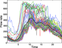
Figure 1: Daily traffic flow trajectories (training data) with the estimated mean function superimposed on the observed trajectories.

1.1 Illustration of traffic flow prediction and the proposed functional data method

Motivated by a practical need for accurate traffic flow prediction, we develop a novel functional data method for predicting future, or unobserved, daily traffic flow for an up-to-date and partially observed traffic flow trajectory. Figure 1 illustrates a sample of daily traffic flow trajectories. The data were collected by a dual loop vehicle detector located near Shea-San Tunnel on National Highway 5 in Taiwan in 2009 and are based on the flow rates (vehicle count per min) over 15-min time intervals, a metric suggested in Highway Capacity Manual 2000 for operational analyses [Zheng, Lee and Shi (2006)]. The trajectories sample 70 days as the training data, while the remaining 14 days are used as the test data to validate the prediction performance. The aim is to predict the unobserved traffic flow trajectory for a partial trajectory with updated flow information up to the “current time” $\tau$, which is given as a time of day. In Figure 2, the raw trajectories (gray lines) before $\tau=8$, 12 and 16:00 are observations from the test data, superimposed on the curves (dotted lines) fitted by functional principal component analysis. After the last observation time point $\tau$, the predicted traffic flow trajectories (solid lines) are obtained by the proposed functional mixture prediction model coupled with the 95% bootstrap prediction intervals. The real data trajectories after times $\tau$ (gray lines) are unobserved in the prediction scenario and are displayed for comparative purposes. The prediction for the trajectory is dynamically updated as the “current time” $\tau$ progresses.

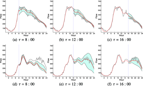
Figure 2: Two samples of trajectories from the test data set [(a)–(c) for Test sample 1; (d)–(f) for Test sample 2]. The fitted curves (dotted lines before times $\tau$) and the predicted curves (solid curves after times $\tau$) with 95% prediction intervals for a partially observed trajectory available up to times $\tau=8$, 12 and 16:00, superimposed on the complete trajectory (gray line).

We note that the aforementioned methods in the literature were largely developed based on “short-term” or “next-step” traffic prediction modeling, where “short-term” refers to a forecast horizon of a time interval. A 15-min interval is commonly used as the forecast horizon for traveler-oriented applications and operational analysis [Zhang and Ye (2008)]. In contrast to the “next-interval” prediction methods in the existing literature, our functional data method is more flexible, as illustrated in Figure 2, allowing valid prediction periods extended from the “current time” to the end of the day and thus providing more information to relevant users.

Since future traffic conditions and temporal traffic flow patterns play a critical role in traffic prediction [e.g., Smith, William and Oswald (2002), Vlahogianni, Karlaftis and Golias (2008)], to take into account distinct daily traffic flow patterns, we propose a functional mixture prediction approach that combines functional prediction with a probabilistic classification procedure. Specifically, we propose to implement functional cluster analysis of past traffic flow trajectories to obtain typical daily traffic flow patterns or clusters, followed by a probabilistic classification for the traffic flow trajectory observed thus far. Based on the traffic flow patterns or clusters identified by the proposed method, we can predict the unobserved traffic flow trajectories by a functional prediction model in conjunction with the estimated posterior membership probabilities of traffic flow clusters. Although motivated by traffic flow analysis and prediction, the proposed methodology is by no means restricted to this particular field and is generally applicable to a wide variety of longitudinally recorded functional data.

In many real applications, clustering of curve data can be challenging and misclassification of an up-to-date and partially observed trajectory can cause loss of prediction accuracy. Hence, a simple “prediction-after-classification” approach based on hard clustering results may not be the best approach. This will be illustrated in our numerical studies including the real data application and simulations. In contrast, the proposed functional mixture prediction framework addresses challenges related to prediction of complex functional data, such as those containing heterogeneous patterns and large variability over time. The proposed functional mixture prediction approach to traffic flow prediction has the following features:

• It is the first approach to employ functional data techniques to address traffic flow prediction applications, which are critical in many intelligent transportation systems.

• The functional data approach allows for interval prediction in contrast to “next-step” traffic flow prediction applications found in the literature.

• The proposed functional mixture prediction model plays a central role in predicting the future trajectory for an up-to-date and partially observed trajectory and takes distinct traffic flow patterns into account to improve prediction accuracy. This study extends the idea of the subspace projected functional clustering method of Chiou and Li (2007) to identify distinct patterns of daily traffic flow from the past data, coupled with the forward functional testing procedure of Li and Chiou (2011) to determine the number of clusters, which lays the groundwork for the functional mixture prediction approach.

• The probabilistic classification approach, including functional clustering and discrimination, is new. It allows for the prediction of posterior membership probabilities using partial information up to the current time, in contrast to clusters constructed by complete trajectories from past data.

• The predictive function in the functional mixture prediction model is built on an existing functional linear model, which is widely used in functional regression modeling [e.g., Ramsay and Dalzell (1991), Müller, Chiou and Leng (2009)] and is easy to implement.

1.2 Literature review of relevant functional data methods

Statistical tools for functional data analysis have been extensively developed during the past two decades to deal with data samples consisting of curves or other infinite-dimensional data objects. Systematic overviews of functional data analysis are provided in the monographs of Ramsay and Silverman (2002, 2005) and Ferraty and Vieu (2006) and in the review articles of Rice (2004), Zhao, Marron and Wells (2004) and Müller (2005, 2009). Functional data analysis provides a wide range of applications in many disciplines. These include biomedical and environmental studies [Di et al. (2009), Gao and Niemeier (2008)], analysis of time-course gene expression profiles [Müller, Chiou and Leng (2008), Coffey and Hinde (2011)], linguistic pitch analysis [Aston, Chiou and Evans (2010)] and demographic and mortality forecasting [Hyndman and Shahid Ullah (2007), Chiou and Müller (2009), D’Amato, Piscopo and Russolillo (2011)], among many others. In relation to functional data prediction, Müller and Zhang (2005) proposed a functional data approach to predicting remaining lifetime and age-at-death distributions from individual event histories observed up to the current time. More recently, Zhou, Serban and Gebraeel (2011) proposed a functional data approach to degradation modeling for the evolution of degradation signals and the remaining life distribution. These are relevant works that contain novel functional data techniques with interesting applications to the prediction of an unobserved event for a partial trajectory observed up to the current time.

Among the various settings in functional regression analysis [Müller (2005)], models with both the response and predictor variables as functions serve this study’s purpose with regard to prediction. Functional regression models of this kind have been considered, for example, in Yao, Müller and Wang (2005b), Chiou and Müller (2007), Müller, Chiou and Leng (2008) and Antoch et al. (2010). Methods of functional data clustering that are found in the literature include the use of multivariate clustering algorithms on the finite-dimensional coefficients of basis function expansions [e.g., Abraham et al. (2003), Serban and Wasserman (2005)], model-based functional data clustering [e.g., James and Sugar (2003), Ma and Zhong (2008)], a general descending hierarchical algorithm [Chapter 9 of Ferraty and Vieu (2006)] and various depth-based classification methods [Cuevas, Febrero and Fraiman (2007), López-Pintado and Romo (2006)], among others. Of particular interest with regard to functional prediction models are the methods that define clusters via subspace projection [Chiou and Li (2007, 2008)]. The subspace projection method considers cluster differences not only in mean functions, but also in eigenfunctions of covariance kernels that takes into account individual random process variations, making it suitable for interpreting the stochastic nature of traffic flow and suggesting a natural link with functional regression models.

This article is organized as follows. In Section 2 we represent traffic flow trajectories as a mixture of stochastic processes and discuss functional clustering and classification methods to take traffic flow patterns into account. Section 3 discusses the functional mixture prediction model, including the algorithm for implementing functional mixture prediction. Sections 4 and 5 illustrate the empirical analysis of traffic flow patterns and results of predicting traffic flow trajectories. Section 6 presents a simulation study to evaluate the performance of the functional mixture prediction in comparison with related methods. Concluding remarks and discussion are provided in Section 7. More information in selecting the number of clusters, the bootstrap prediction intervals and additional details in the simulation design and results are deferred to Supplementary Materials [Chiou (2012)].

2 Modeling traffic flow trajectories and clustering traffic flow patterns

Previous studies in traffic flow prediction and modeling have revealed that traffic condition data is characteristically stochastic, as opposed to chaotic [Smith, William and Oswald (2002)]. The stochastic features of traffic flow trajectories are suggestive of a functional data approach. In the functional data framework, we adopt the notion that each daily traffic flow trajectory is a realization of a random function sampled from a mixture of stochastic processes. Let $Z$ denote the random function for the daily traffic flow trajectory in the domain $\mathcal{U}=[0,T]$. Here, the random function $Z$ is square integrable with the inner product of any two functions $f_{1}$ and $f_{2}$ defined as $\langle f_{1},f_{2}\rangle_{\mathcal{U}}=\int_{\mathcal{U}}f_{1}(t)f_{2}(t)\,dt$ with the norm $\|f_{1}\|_{\mathcal{U}}=\langle f_{1},f_{1}\rangle_{\mathcal{U}}^{{1}/{2}}$. It is assumed that the random function $Z(t)$ has a smooth mean function $EZ(t)=\mu_{Z}(t)$ and covariance function $\operatorname{cov}(Z(s),Z(t))=G_{Z}(s,t)$, for $s$ and $t$ in $\mathcal{U}$.

2.1 Functional clustering of historical traffic flow trajectories

While temporal traffic flow patterns are critical in traffic prediction, the underlying traffic flow structures and number of typical patterns are unknown and remain to be explored. We assume the mixture process $Z$ consists of $K$ subkprocesses, with each subprocess corresponding to a cluster. The random cluster variable $C$ for each individual cluster membership is randomly distributed among clusters with label $c\in\{1,\ldots,K\}$. For each subprocess associated with cluster $c$, define the conditional mean function $E(Z(t)\mid C=c)=\mu^{(c)}(t)$ and covariance function $\operatorname{cov}(Z(s),Z(t)\mid C=c)=G^{(c)}(s,t)$, for $c\in\{1,\ldots,K\}$. Let $(\lambda^{(c)}_{j},\varphi^{(c)}_{j})$ be the corresponding eigenvalue–eigenfunction pairs of the covariance kernel $G^{(c)}$, where $\lambda^{(c)}_{j}$ are in nonascending order. Assume, under mild conditions, each subprocess possesses a Karhunen–Loève expansion for the daily traffic flow trajectory $Z$ given by

$${Z}^{(c)}(t)=\mu^{(c)}(t)+\sum_{j=1}^{\infty}{\xi}^{(c)}_{j}\varphi^{(c)}_{j}(t),$$ (1)

where ${\xi}^{(c)}_{j}=\langle Z-\mu^{(c)},\varphi^{(c)}_{j}\rangle_{\mathcal{U}}$ with $\langle\varphi^{(c)}_{j},\varphi^{(c)}_{l}\rangle_{\mathcal{U}}=1$ for $j=l$ and 0 otherwise. In practice, it is often the case that the representation only requires a small number of components to approximate the trajectories. In general, trajectories with simpler structure require fewer components as compared to more complex trajectories.

Following the conventional approach, the best cluster membership $c^{*}$ given $Z$ is determined by maximizing the posterior probability $P_{C\mid Z}(\cdot\mid\cdot)$ such that

$$c^{*}(Z)=\mathop{\operatorname{arg\,max}}_{c\in\{1,\ldots,K\}}P_{C\mid Z}(c\mid Z).$$ (2)

We propose estimating the posterior membership probability $P(C=c\mid Z)$ using the so-called discriminative approach, as opposed to the generative approach [see, e.g., Dawid (1976), Bishop and Lasserre (2007)]. While there is no general consensus for choosing between generative and discriminative approaches [Ng and Jordan (2002), Xue and Titterington (2008)], the former requires a priori knowledge on the class-conditional probability density functions, information that is difficult to justify incorporating for the traffic flow trajectories. It is easier to use the discriminative approach that directly estimates the class-membership probabilities without attempting to model the underlying probability distributions of the random functions. Following this line, the multiclass logit model is a popular method for estimating the posterior membership probabilities. We propose incorporating a distance measure between $Z$ and its projection associated with each cluster as the covariate in the multiclass logit model.

Consider the relative $L^{2}$ distance as the distance measure based on cluster subspace projection as

$$d^{(c)}=\frac{\|Z-\tilde{Z}^{(c)}\|^{2}}{\sum_{k=1}^{K}\|Z-\tilde{Z}^{(k)}\|^{2}},$$ (3)

where $\tilde{Z}^{(c)}(t)=\mu^{(c)}(t)+\sum_{l=1}^{M_{c}}{\xi}_{l}^{(c)}\varphi_{l}^{(c)}(t)$, with ${\xi}_{l}^{(c)}=\langle Z-\mu^{(c)},\varphi^{(c)}_{l}\rangle_{\mathcal{U}}$. The value $M_{c}$ is finite and is chosen data-adaptively so that $Z$ is well approximated by $Z^{(c)}$ by the $M_{c}$ components. Let $\mathbf{d}=(1,d^{(1)},\ldots,d^{(K-1)})^{\top}$ and $\bolds{\gamma}_{c}=(\gamma_{0c},\gamma_{1c},\ldots,\gamma_{(K-1)c})^{\top}$. Taking the vector $\mathbf{d}$ as the covariate, we can estimate the posterior cluster membership probability using the multiclass logit model,

$$P(C=c\mid Z)=\frac{\exp\{\bolds{\gamma}_{c}^{\top}\mathbf{d}\}}{\sum_{k=1}^{K}\exp\{\bolds{\gamma}_{k}^{\top}\mathbf{d}\}}$$ (4)

for $c=1,\ldots,K-1$ and $P(C=K\mid Z)=1-\sum_{c=1}^{K-1}P(C=c\mid Z)$ with the $K$th cluster being the baseline. The vector of regression coefficients $\bolds{\gamma}_{c}$ remains to be estimated.

Clusters defined by criterion (2) are based on subspace projection. Let $S^{(c)}_{M}$ be the linear span of the set of eigenfunctions $\{\varphi_{1}^{(c)},\ldots,\varphi_{M_{c}}^{(c)}\}$, $c=1,\ldots,K$. For identifiability, it is assumed that for any two clusters $c$ and $d$ the following two conditions do not hold simultaneously: (i) $S^{(c)}_{M}$ belongs to $S^{(d)}_{M}$, (ii) $\mu^{(c)}=\mu^{(d)}$, or $\mu^{(c)}\in S^{(d)}_{M}$ and $\mu^{(d)}\in S^{(c)}_{M}$. These conditions were derived in Theorem 1 of Chiou and Li (2007) for identifiability of clusters defined via subspace projection. Criterion (2) leads to clusters with similar curves that are embedded in the cluster subspace spanned by the cluster center components, the mean function and the eigenfunctions of the covariance kernel that represent the functional principal component subspace.

In addition, the number of clusters is unknown, and must be determined in practice. The method used to determine the number of clusters in this study is based on a sequence of tests on cluster structures done to ensure statistical significance in the difference between cluster types as proposed in Li and Chiou (2011). The number of clusters $K$ is determined by testing a sequence of null hypotheses $H_{01}\dvtx\mu^{(c)}=\mu^{(d)}$ and $H_{02}\dvtx S^{(c)}_{M}=S^{(d)}_{M}$, for $1\leq c\neq d\leq K$. The forward functional testing procedure aims to search for the maximum number of clusters while retaining differences with statistical significance among the clusters. The procedure is especially suitable for the subspace projected functional clustering method. The sequence of the functional hypothesis tests helps identify significant differences between cluster structures and provides additional insight into further cluster analysis. Since the hypothesis tests are based on bootstrap resampling methods, it takes substantial computational time to construct the reference distribution. Details of the procedure are discussed in Li and Chiou (2011) and we have briefly summarized them in Supplementary Material A [Chiou (2012)].

2.2 Probabilistic functional classification of traffic flow patterns

For the purpose of prediction, the time domain $\mathcal{U}$ of the process $Z$ is decomposed into two exclusive time domains ${\mathcal{S}(\tau)}=[0,\tau]$ and ${\mathcal{T}(\tau)}=[\tau,T]$. Now, let $Z^{*}$ be a newly observed trajectory of the process $Z$, denoted by $Z_{\mathcal{S}(\tau)}^{*}$ as observed up to time $\tau$. We predict the cluster membership probability of the trajectory $Z^{*}$ based on the known trajectory $Z_{{\mathcal{S}(\tau)}}^{*}$ observed until time $\tau$, which will then be used to predict the unobserved trajectory $Z_{{\mathcal{T}(\tau)}}^{*}$.

We define the relative $L^{2}$ distance in a manner similar to (3) via cluster subspace projection, but it is based on the partially observed $Z_{{\mathcal{S}(\tau)}}^{*}$ rather than the entire $Z^{*}$ since the part $Z_{{\mathcal{T}(\tau)}}^{*}$ is not yet observed. Suppose that the cluster subspaces $\mu^{(c)}$ and $\{\varphi_{{\mathcal{S}(\tau)},j}^{(c)}\}$, $c=1,\ldots,K$, are being identified as in Section 2.1. Then, the relative $L^{2}$ distance is defined as

$$d_{\mathcal{S}(\tau)}^{*(c)}=\frac{\|Z_{{\mathcal{S}(\tau)}}^{*}-\tilde{Z}_{\mathcal{S}(\tau)}^{*(c)}\|^{2}}{\sum_{k=1}^{K}\|Z_{{\mathcal{S}(\tau)}}^{*}-\tilde{Z}_{\mathcal{S}(\tau)}^{(k)}\|^{2}},$$ (5)

where $\tilde{Z}_{\mathcal{S}(\tau)}^{*(c)}(s)=\mu^{(c)}(s)+\sum_{l=1}^{M_{c}}{\xi}_{{\mathcal{S}(\tau)},l}^{*(c)}\varphi_{{\mathcal{S}(\tau)},l}^{(c)}(s)$, with ${\xi}_{{\mathcal{S}(\tau)},l}^{*(c)}=\langle Z_{\mathcal{S}(\tau)}^{*}-\mu^{(c)},\break\varphi^{(c)}_{{\mathcal{S}(\tau)},l}\rangle_{{\mathcal{S}(\tau)}}$. Here, the set of eigenfunctions $\{\varphi^{(c)}_{{\mathcal{S}(\tau)},l}\}$ corresponds to the covariance kernel $G^{(c)}_{{\mathcal{S}(\tau)}}$ of the random process $Z_{{\mathcal{S}(\tau)}}$. Taking $\mathbf{d}_{\mathcal{S}(\tau)}^{*}=(1,d_{\mathcal{S}(\tau)}^{*(1)},\ldots,\break d_{\mathcal{S}(\tau)}^{*(K-1)})^{\top}$ as the covariate, we can predict the cluster membership probability based on the newly observed $Z^{*}_{\mathcal{S}(\tau)}$ using the multiclass logit model

$$P\bigl{(}C=c\mid Z_{\mathcal{S}(\tau)}^{*}\bigr{)}=\frac{\exp\{\bolds{\gamma}_{c}^{\top}\mathbf{d}_{\mathcal{S}(\tau)}^{*}\}}{\sum_{k=1}^{K}\exp\{\bolds{\gamma}_{k}^{\top}\mathbf{d}_{\mathcal{S}(\tau)}^{*}\}}$$ (6)

for $c=1,\ldots,K-1$, and $P(C=K\mid Z_{\mathcal{S}(\tau)}^{*})=1-\sum_{c=1}^{K-1}P(C=c\mid Z_{\mathcal{S}(\tau)}^{*})$ with the $K$th cluster being baseline. We note that the vector of coefficients $\bolds{\gamma}_{c}$ here is the same as that in (4) based on the historical or training data.

2.3 Estimation for probabilistic functional classification

In practice, the observed trajectories may be contaminated with random measurement errors. Let $Y_{i}(t_{ij})$ be the $j$th observation of the $i$th individual flow trajectory from the underlying process $Z_{i}^{(c)}$ of cluster $c$ observed at time $t_{ij}$, $0\leq t_{ij}\leq T$, such that $Y_{i}(t_{ij})=Z_{i}^{(c)}(t_{ij})+\epsilon_{ij}$, where $Z_{i}^{(c)}$ is the underlying random function such that $Z_{i}^{(c)}(t)=\mu^{(c)}(t)+\sum_{k=1}^{\infty}{\xi}_{ki}^{(c)}\varphi_{k}^{(c)}(t)$, and the random measurement errors $\epsilon_{ij}$ are independent of ${\xi}_{ki}^{(c)}$ with mean zero and variance $\sigma^{2}$.

To identify the structures of cluster subspaces, $\{\hat{\mu}^{(c)},\{\hat{\varphi}_{k}^{(c)}\}_{k=1,\ldots,M_{c},}\}$, $c=1,\ldots,K$, we follow the idea of defining clusters via subspace projection and apply the proposed subspace-projected functional clustering procedure to the training data set. In the initial step, since cluster membership is unknown, the clustering is based on functional principal component scores of an overall single random process. Details of the initial clustering refer to Section 2.2.1 of Chiou and Li (2007). In the iterative updating step, cluster membership is determined by criterion (2) in a hard clustering manner. The clustering procedure is implemented iteratively in identifying between (i) cluster subspaces and (ii) cluster memberships until convergence.

Cluster subspaces

Given the observations $\{(t_{ij},Y_{i}(t_{ij})),i=1,\ldots,n,j=1,\ldots,m\}$, from the historical or training data, and the cluster memberships of the trajectories, using the observations belonging to cluster $c$, the mean function $\mu^{(c)}$ can be estimated by applying the locally weighted least squares method while the estimates of the components $\varphi^{(c)}_{k}$ and ${\xi}^{(c)}_{ik}$ rely on the covariance estimate $\hat{G}^{(c)}$ by applying the smoothing scatterplot data $(Y_{ij}-\hat{\mu}^{(c)}(t_{ij}))(Y_{il}-\hat{\mu}^{(c)}(t_{il}))$ to fit a local linear plane. Details of this estimation can be found in Chiou, Müller and Wang (2003) and Yao, Müller and Wang (2005a), for example. The smoothing parameters in the mean and covariance estimation steps are chosen data-adaptively via the 10-fold cross-validation method. An estimate of ${\xi}^{(c)}_{ik}$ can be obtained by the conditional expectation approach of Yao, Müller and Wang (2005a) for the case of sparse designs. Here, we simply obtain the estimate $\hat{\xi}^{(c)}_{ik}=\langle Y_{i}-\hat{\mu}^{(c)},\hat{\varphi}_{k}{(c)}\rangle_{\mathcal{U}}$ by numerical approximation for the case of dense designs of traffic flow recording. The value $M_{c}$ is selected as the minimum that reaches a certain level of the proportion of total variance explained by the $M_{c}$ leading components such that

$$M_{c}=\mathop{\operatorname{arg\,min}}_{L:L\geq 1}\Biggl{\{}\sum_{l=1}^{L}\hat{\lambda}_{l}^{(c)}\bigg{/}\sum_{l=1}^{\infty}\hat{\lambda}_{l}^{(c)}1_{\{\hat{\lambda}_{l}^{(c)}>0\}}\geq\delta\Biggr{\}},$$ (7)

where $\delta=90\%$ in this study. These cluster structure estimates are used in turn to estimate the vector of regression coefficients $\bolds{\gamma}_{k}$ in (8) below.

Cluster memberships

Given the structure of each cluster based on the training data, we then use the discriminative approach to fit the posterior probabilities of cluster membership $P(C=c\mid Y_{i})$ such that

$$\hat{P}(C=c\mid Y_{i})=\frac{\exp\{\hat{\bolds{\gamma}}_{c}^{\top}\hat{\mathbf{d}}_{i}\}}{\sum_{k=1}^{K}\exp\{\hat{\bolds{\gamma}}_{k}^{\top}\hat{\mathbf{d}}_{i}\}},\qquad c=1,\ldots,K-1,$$ (8)

and $\hat{P}(C=K\mid Y_{i})=1-\sum_{k=1}^{K-1}\hat{P}(C=k\mid Y_{i})$, taking the $K$th cluster as the baseline. Here, the relative $L^{2}$ distance vector $\hat{\mathbf{d}}_{i}=(1,\hat{d}_{i}^{(1)},\ldots,\hat{d}_{i}^{(K-1)})^{\top}$ serves as the predictor variable and is calculated by

$$\hat{d}_{i}^{(c)}=\frac{\|Y_{i}-\hat{Z}_{i}^{(c)}\|^{2}}{\sum_{k=1}^{K}\|Y_{i}-\hat{Z}_{i}^{(k)}\|^{2}},\qquad c=1,\ldots,K-1,$$ (9)

where $\hat{Z}_{i}^{(c)}(s)=\hat{\mu}^{(c)}(s)+\sum_{j=1}^{M_{c}}\hat{\xi}_{ij}^{(c)}\hat{\varphi}_{j}^{(c)}(s)$, with $\hat{\xi}^{(c)}_{ij}$ defined above. The coefficient estimates $\hat{\bolds{\gamma}}_{c}=(\gamma_{0c},\gamma_{1c},\ldots,\gamma_{(K-1)c})$ are obtained by the conventional iterated reweighted least squares method [McCullagh and Nelder (1983)]. The resulting estimate (8) is used to determine the cluster membership according to (2).

Now, given a newly observed trajectory $Y^{*}$ up to time $\tau$, denoted by $Y^{*}_{{\mathcal{S}(\tau)}}$, we obtain the covariate vector $\hat{\mathbf{d}}_{\mathcal{S}(\tau)}^{*}=(1,\hat{d}_{\mathcal{S}(\tau)}^{*(1)},\ldots,\hat{d}_{\mathcal{S}(\tau)}^{*(K-1)})^{\top}$, where

$$\hat{d}_{\mathcal{S}(\tau)}^{*(c)}=\frac{\|Y_{{\mathcal{S}(\tau)}}^{*}-\hat{Z}_{{\mathcal{S}(\tau)}}^{*(c)}\|^{2}}{\sum_{k=1}^{K}\|Y_{{\mathcal{S}(\tau)}}^{*}-\hat{Z}_{{\mathcal{S}(\tau)}}^{(k)}\|^{2}},\qquad c=1,\ldots,K-1.$$ (10)

Here, $\hat{Z}_{{\mathcal{S}(\tau)}}^{*(c)}(s)=\hat{\mu}^{(c)}(s)+\sum_{j=1}^{M_{c}}\hat{\xi}_{{\mathcal{S}(\tau)},j}^{*(c)}\hat{\varphi}_{{\mathcal{S}(\tau)},j}^{(c)}(s)$, and $\hat{\xi}^{*(c)}_{{\mathcal{S}(\tau)},j}$ can be obtained by a numerical approximation to $\langle Z^{*}_{{\mathcal{S}(\tau)}}-\hat{\mu}_{{\mathcal{S}(\tau)}}^{(c)},\hat{\varphi}_{{\mathcal{S}(\tau)},j}^{(c)}\rangle_{{\mathcal{S}(\tau)}}$. To obtain$\{\hat{\varphi}_{{\mathcal{S}(\tau)},j}^{(c)}\}$, we simply decompose the covariance estimate $\hat{C}^{(c)}$ into blocks corresponding to the time domains ${\mathcal{S}(\tau)}$ and ${\mathcal{T}(\tau)}$ without re-estimating the covariance function, making the dynamical prediction step easy to implement for any given $\tau$. We predict the cluster membership for the newly observed $Y^{*}_{\mathcal{S}(\tau)}$ by the posterior probability

$$\quad\hat{P}\bigl{(}C=c\mid Y_{{\mathcal{S}(\tau)}}^{*}\bigr{)}=\frac{\exp\{\hat{\bolds{\gamma}}_{c}^{\top}\hat{\mathbf{d}}_{\mathcal{S}(\tau)}^{*}\}}{\sum_{k=1}^{K}\exp\{\hat{\bolds{\gamma}}_{k}^{\top}\hat{\mathbf{d}}_{\mathcal{S}(\tau)}^{*}\}},\qquad c=1,\ldots,K-1,$$ (11)

and $\hat{P}(C=K\mid Y_{{\mathcal{S}(\tau)}}^{*})=1-\sum_{c=1}^{K-1}\hat{P}(C=c\mid Y_{{\mathcal{S}(\tau)}}^{*})$.

3 Functional mixture prediction of future traffic flow trajectories

To accurately predict traffic flow trajectories under various traffic conditions, we combine the functional prediction model with functional clustering and classification methods. Given a newly observed trajectory $Z_{\mathcal{S}(\tau)}^{*}$ of the process $Z$ as observed up to time $\tau$, we propose a functional mixture prediction model to predict the trajectory of $Z^{*}$ on the time interval ${\mathcal{T}(\tau)}=[\tau,T]$, denoted by $Z_{{\mathcal{T}(\tau)}}^{*}$ as

$$E\bigl{(}Z_{{\mathcal{T}(\tau)}}^{*}(t)\mid Z_{{\mathcal{S}(\tau)}}^{*}\bigr{)}=\sum_{c=1}^{K}P\bigl{(}C=c\mid Z_{{\mathcal{S}(\tau)}}^{*}\bigr{)}\tilde{Z}_{{\mathcal{T}(\tau)}}^{*(c)}(t),$$ (12)

where $\tilde{Z}_{{\mathcal{T}(\tau)}}^{*(c)}(t)=E(Z^{*}_{{\mathcal{T}(\tau)}}(t)\mid Z_{{\mathcal{S}(\tau)}}^{*},C=c)$ is the predictive function conditional on cluster $C=c$, and $P(C=c\mid Z_{{\mathcal{S}(\tau)}}^{*})$ is the posterior probability of cluster membership given the newly observed trajectory $Z_{{\mathcal{S}(\tau)}}^{*}$ up to time $\tau$. The functional mixture prediction model (12), obtained by the law of iterated expectation on the random cluster membership variable $C$, $E\{E(Z_{{\mathcal{T}(\tau)}}^{*}(t)\mid Z_{{\mathcal{S}(\tau)}}^{*},C)\}$, minimizes the expected risk, $E\{\mathcal{L}(Z_{{\mathcal{T}(\tau)}}^{*},\widetilde{Z}_{{\mathcal{T}(\tau)}}^{C})\}$, where $\widetilde{Z}_{{\mathcal{T}(\tau)}}^{C}(t)=E(Z^{*}_{{\mathcal{T}(\tau)}}(t)\mid Z_{{\mathcal{S}(\tau)}}^{*},C)$ and the loss function is defined as $\mathcal{L}(Z_{{\mathcal{T}(\tau)}}^{*},\widetilde{Z}_{{\mathcal{T}(\tau)}}^{c})=\int_{{\mathcal{T}(\tau)}}\{Z_{{\mathcal{T}(\tau)}}^{*}(t)-\tilde{Z}_{{\mathcal{T}(\tau)}}^{*(c)}(t)\}^{2}\,dt$.

3.1 Functional linear regression of traffic flow trajectories

In a regression setting, the process $Z(s)$, for $s\in{\mathcal{S}(\tau)}$ denoted by $Z_{\mathcal{S}(\tau)}$, serves as the predictor function and the process $Z(t)$, for $t\in{\mathcal{T}(\tau)}$ denoted by $Z_{\mathcal{S}(\tau)}$, is the response function. The subspace projected functional clustering method developed above is well suited to identifying clusters in conjunction with functional prediction. For each cluster subspace, $Z^{(c)}$ is decomposed into $Z_{{\mathcal{S}(\tau)}}^{(c)}(s)$ and $Z_{{\mathcal{T}(\tau)}}^{(c)}(t)$ whose Karhunen–Loève expansions can be obtained such that $Z_{\mathcal{S}(\tau)}^{(c)}(s)=\mu^{(c)}(s)+\sum_{j=1}^{\infty}\xi_{{\mathcal{S}(\tau)},j}^{(c)}\varphi_{{\mathcal{S}(\tau)},j}^{(c)}(s)$ and $Z_{\mathcal{T}(\tau)}^{(c)}(t)=\mu^{(c)}(t)+\sum_{j=1}^{\infty}\xi_{{\mathcal{T}(\tau)},j}^{(c)}\varphi_{{\mathcal{T}(\tau)},j}^{(c)}(t)$, where the notation $\xi_{{\mathcal{S}(\tau)},j}^{(c)}$, $\varphi_{{\mathcal{S}(\tau)},j}^{(c)}$, $\xi_{{\mathcal{T}(\tau)},j}^{(c)}$ and $\varphi_{{\mathcal{T}(\tau)},j}^{(c)}$ are defined analogously to those on the entire domain $\mathcal{U}$, but they correspond to the sub-domains ${\mathcal{S}(\tau)}$ and ${\mathcal{T}(\tau)}$.

We consider a functional linear regression model [e.g., Ramsay and Dalzell (1991), Müller, Chiou and Leng (2008)] conditional on cluster membership,

$$E\bigl{(}Z_{\mathcal{T}(\tau)}(t)\mid Z_{\mathcal{S}(\tau)},C=c\bigr{)}$$

(13)

$$\qquad=\mu^{(c)}(t)+\int_{\mathcal{S}(\tau)}\beta_{\tau}^{(c)}(s,t)\bigl{\{}Z_{\mathcal{S}(\tau)}(s)-\mu^{(c)}(s)\bigr{\}}\,ds$$

for all $t\in{\mathcal{T}(\tau)}$. Here, given a fixed value of $\tau$, assume the bivariate regression function $\beta_{\tau}^{(c)}(s,t)$ is smooth and square integrable, that is,$\int_{{\mathcal{T}(\tau)}}\int_{{\mathcal{S}(\tau)}}\beta_{\tau}^{(c)}(s,t)\,ds\,dt<\infty$. Under the smoothness assumption on the underlying random process, we further assume that the bivariate regression function $\beta_{\tau}^{(c)}(s,t)$ is a smooth function of $\tau$ for all $s$ and $t$. Using the eigenbasis expansion for the regression coefficient function such that $\beta_{\tau}^{(c)}(s,t)=\sum_{k=1}^{\infty}\sum_{j=1}^{\infty}\beta_{\tau,kj}^{(c)}\varphi_{{\mathcal{S}(\tau)},j}^{(c)}(s)\varphi_{{\mathcal{T}(\tau)},k}^{(c)}(t)$, model (3.1) can be expressed as

$$\qquad E\bigl{(}Z_{\mathcal{T}(\tau)}(t)\mid Z_{\mathcal{S}(\tau)},C=c\bigr{)}=\mu^{(c)}(t)+\sum_{j=1}^{\infty}\sum_{k=1}^{\infty}\beta_{\tau,kj}^{(c)}\xi_{{\mathcal{S}(\tau)},j}^{(c)}\varphi_{{\mathcal{T}(\tau)},k}^{(c)}(t),$$ (14)

where $\xi_{{\mathcal{S}(\tau)},j}^{(c)}=\langle Z_{\mathcal{S}(\tau)}-\mu^{(c)},\varphi_{{\mathcal{S}(\tau)},j}^{(c)}\rangle_{{\mathcal{S}(\tau)}}$ and $\beta_{\tau,kj}^{(c)}={E(\xi_{{\mathcal{S}(\tau)},j}^{(c)}\xi_{{\mathcal{T}(\tau)},k}^{(c)})}/\break{E\{(\xi_{{\mathcal{S}(\tau)},j}^{(c)})^{2}\}}$ are the regression parameters to be estimated. Under the smoothness assumption on $\beta_{\tau}^{(c)}(s,t)$ along with $\tau$, it follows that $\beta_{\tau,kj}^{(c)}$ is also smooth in $\tau$ for all $k$ and $j$.

3.2 Functional linear prediction model for future traffic flow

Given $Z_{{\mathcal{S}(\tau)}}^{*}$, we aim to predict the values of $Z_{{\mathcal{T}(\tau)}}^{*}$. Suppose that the cluster structures $\mu^{(c)}$ and $\{\varphi_{{\mathcal{S}(\tau)},j}^{(c)}\}$ and the regression coefficients $\beta_{\tau,kj}^{(c)}$ are given. In practice, these estimates can be obtained from the functional clustering and the functional regression analysis using the historical or training data as described in Section 2. Then, the functional prediction model below is used to predict the unobserved trajectory conditional on a specific cluster:

$$\quad E\bigl{(}Z^{*}_{\mathcal{T}(\tau)}(t)\mid Z^{*}_{\mathcal{S}(\tau)},C=c\bigr{)}=\mu^{(c)}(t)+\sum_{j=1}^{\infty}\sum_{k=1}^{\infty}\beta_{\tau,kj}^{(c)}\xi_{{\mathcal{S}(\tau)},j}^{*(c)}\varphi_{{\mathcal{T}(\tau)},k}^{(c)}(t)$$ (15)

for all $t\in{\mathcal{T}(\tau)}$, where $\xi_{{\mathcal{S}(\tau)},j}^{*(c)}=\langle Z_{\mathcal{S}(\tau)}^{*}-\mu^{(c)},\varphi_{{\mathcal{S}(\tau)},j}^{(c)}\rangle_{{\mathcal{S}(\tau)}}$ and will be obtained by numerical approximation.

Finally, given a partially observed trajectory $Z^{*}_{{\mathcal{S}(\tau)}}$, the unobserved trajectory $Z^{*}_{{\mathcal{T}(\tau)}}$ can be predicted by the functional mixture prediction model (12) using the results of the functional prediction model (15) in conjunction with the multiclass logit model (6). However, the components in these models remain to be estimated. The estimation procedure for the functional linear model is briefly summarized below.

3.3 Estimation for functional mixture prediction models

We note that the estimation of $\beta_{\tau,kj}$ in (14) and (15) can further be simplified using a simple linear regression approach [Müller, Chiou and Leng (2008)], such that

$$E\bigl{(}\xi_{{\mathcal{T}(\tau)},k}^{(c)}\mid\xi_{{\mathcal{S}(\tau)},j}^{(c)}\bigr{)}=\beta_{\tau,kj}^{(c)}\xi_{{\mathcal{S}(\tau)},j}^{(c)}$$

for all pairs of $(k,j)$. Therefore, functional linear regression can be decomposed into a series of simple linear regressions of functional principal component scores of the response processes in relation to those of the predictor processes.

For our predictions, given the cluster membership information and the subspace structure of each cluster, we estimate $\beta_{\tau}^{(c)}(s,t)$ in the functional linear regression model (3.1) based on the training data. Given the estimated principal component functions $\hat{\varphi}_{{\mathcal{S}(\tau)},j}^{(c)}(t)$ and $\hat{\varphi}_{{\mathcal{T}(\tau)},k}^{(c)}(t)$ and the principal component scores $\hat{\xi}_{{\mathcal{S}(\tau)},j}^{(c)}$ and $\hat{\xi}_{{\mathcal{T}(\tau)},k}^{(c)}$, the estimate of $\beta_{\tau,kj}^{(c)}$ can be obtained by

$$\qquad\tilde{\beta}_{\tau,kj}^{(c)}=\bigl{\{}(n_{c}-1)\lambda_{{\mathcal{S}(\tau)},j}^{(c)}\bigr{\}}^{-1}\sum_{i=1}^{n_{c}}\bigl{(}\hat{\xi}_{{\mathcal{S}(\tau)},i,j}^{(c)}-\overline{\xi}_{{\mathcal{S}(\tau)},j}^{(c)}\bigr{)}\bigl{(}\hat{\xi}_{{\mathcal{T}(\tau)},i,k}^{(c)}-\overline{\xi}_{{\mathcal{T}(\tau)},k}^{(c)}\bigr{)},$$ (16)

where $\overline{\xi}_{{\mathcal{S}(\tau)},j}^{(c)}$ and $\overline{\xi}_{{\mathcal{T}(\tau)},k}^{(c)}$ are sample averages of $\hat{\xi}_{{\mathcal{S}(\tau)},i,j}^{(c)}$ and $\hat{\xi}_{{\mathcal{T}(\tau)},i,k}^{(c)}$, respectively.

To take advantage of smoothness in prediction as the value $\tau$ progresses, we further smooth the estimates $\{\tilde{\beta}_{\tau,kj}^{(c)},\tau=\tau_{1},\ldots,\tau_{Q}\}$ over $\tau$ to obtain the smooth estimates $\hat{\beta}_{\tau,kj}^{(c)}$, where $Q$ is the number of time points at which predicting the future trajectory is of interest. Here, we use the local linear smoothing method with cross-validated bandwidth [see, e.g., Fan and Gijbels (1996)]. Accordingly, using $\hat{\beta}_{\tau,kj}^{(c)}$ and the estimates $\hat{\mu}^{(c)}(t)$ and $\hat{\varphi}_{{\mathcal{T}(\tau)},k}^{(c)}(t)$, we obtain the predicted trajectory conditional on cluster $c$ by

$$\hat{Z}^{*(c)}_{\mathcal{T}(\tau)}(t) = \hat{E}\bigl{(}Z^{*}_{\mathcal{T}(\tau)}(t)\mid Y^{*}_{\mathcal{S}(\tau)},C=c\bigr{)}$$

$$= \hat{\mu}^{(c)}(t)+\sum_{j=1}^{M_{c}}\sum_{k=1}^{M_{c}}\hat{\beta}_{\tau,kj}^{(c)}\hat{\xi}_{{\mathcal{S}(\tau)},j}^{*(c)}\hat{\varphi}_{{\mathcal{T}(\tau)},k}^{(c)}(t)$$

for all $t\in{\mathcal{T}(\tau)}$. Here, $M_{c}$ is determined by (7). Finally, combining the results of (3.3) with (11), we obtain the predicted unobserved traffic flow trajectory

$$\hat{Z}^{*}_{\mathcal{T}(\tau)}(t)=\hat{E}\bigl{(}Z_{{\mathcal{T}(\tau)}}^{*}(t)\mid Y_{{\mathcal{S}(\tau)}}^{*}\bigr{)}=\sum_{c=1}^{K}\hat{Z}^{*(c)}_{\mathcal{T}(\tau)}(t)\hat{P}\bigl{(}C=c\mid Y_{{\mathcal{S}(\tau)}}^{*}\bigr{)}.$$ (18)

3.4 Implementation algorithm of functional mixture predictions

Suppose there is a newly observed trajectory $\{(t^{*}_{j},Y^{*}(t^{*}_{j}));t^{*}_{j}<\tau\}$, denoted by $Y^{*}_{{\mathcal{S}(\tau)}}$ for short. The algorithm for functional mixture prediction that combines the functional classification procedure with the functional prediction model is summarized as follows.

1. []

2. Identification of cluster subspaces. Perform the subspace-projected functional clustering procedure according to criterion (2) to identify cluster subspaces, $\{\hat{\mu}^{(c)},\{\hat{\varphi}_{k}^{(c)}\}_{k=1,\ldots,M_{c}}\}$, $c=1,\ldots,K$, based on the training data set as discussed in Sections 2.1 and 2.3.

3. Model fitting based on the historical or training data.

   1. [(ii)]

   2. Obtain the multiclass logit model for cluster membership distributions. Obtain from Step 1 the regression coefficient estimates $\hat{\bolds{\gamma}}_{c}$ in (8).

   3. Fit the functional linear regression model. Fit the cluster-specific functional linear regression models and obtain the regression coefficient estimates $\hat{\beta}_{\tau,kj}^{(c)}$ as a smoothed version of (16).

4. Prediction of the future traffic flow trajectory for a new and partially observed $Y^{*}_{{\mathcal{S}(\tau)}}$ conditional on clusters.

   1. [(ii)]

   2. Predict the posterior membership probability of $Y^{*}_{{\mathcal{S}(\tau)}}$ associated with each cluster. Calculate the relative $L^{2}$ distances $d_{\mathcal{S}(\tau)}^{*(c)}$ for the given $Y^{*}_{{\mathcal{S}(\tau)}}$ in (10) and obtain the posterior probability $\hat{\operatorname{Pr}}(C=c\mid Y_{\mathcal{S}(\tau)}^{*})$ in (11).

   3. Predict the unobserved trajectory $Y_{\mathcal{T}(\tau)}^{*}$ conditioning on each of the clusters. Obtain the cluster-specific functional prediction model fit $\hat{E}(Y_{\mathcal{T}(\tau)}^{*}\mid Y_{\mathcal{S}(\tau)}^{*},C=c)$ in (3.3).

5. Prediction of traffic flow trajectory by the functional mixture prediction model. Calculate the predicted trajectory $\hat{E}(Y_{\mathcal{T}(\tau)}^{*}\mid Y_{\mathcal{S}(\tau)}^{*})$ in (18) using the results of $\hat{\operatorname{Pr}}(C=c\mid Y_{\mathcal{S}(\tau)}^{*})$ and $\hat{E}(Y_{\mathcal{T}(\tau)}^{*}\mid Y_{\mathcal{S}(\tau)}^{*},C=c)$ and obtain the bootstrap prediction intervals.

Details in constructing the bootstrap prediction intervals in Step 4 are provided in Supplementary Material B [Chiou (2012)].

4 Analysis of traffic flow patterns

The sample data set of daily traffic flow trajectories from Section 1.1 is divided into a training data set (70 days) and a test data set (14 days) to examine the predictive performance of our model. Clusters of the traffic flow patterns from the training data are identified based on subspace projection using the proposed subspace-projected functional clustering method according to criterion (2). The implementation of the functional forward testing procedure of Li and Chiou (2011) leads to the choice of 3 clusters. Table 1 summarizes the empirical probabilities of rejecting the null hypotheses for $K=2,3,4$, based on 200 bootstrap samples. The $p$-values with reference to the predetermined level of significance 0.05, adjusted for multiple comparisons, indicate that when $K=2$ and 3, the clusters are all significantly distinct, while Clusters 1 and 4 when $K=4$ are not significantly different in terms of the mean functions and the eigenspaces.

Table 1: Empirical probabilities of rejecting the null hypotheses $H_{01}$ and $H_{02}$, respectively, based on 200 bootstrap samples

Number of clusters	Clusters	$\bolds{H_{01}\dvtx\mu^{(c)}=\mu^{(d)}}$	$\bolds{H_{02}\dvtx S^{(c)}=S^{(d)}}$
$2$	1 vs. 2	$0.000$	$0.010$
$3$	1 vs. 2	$0.000$	$0.005$
	1 vs. 3	$0.000$	$0.005$
	2 vs. 3	$0.005$	$0.015$
$4$	1 vs. 2	$0.000$	$0.055$
	1 vs. 3	$0.000$	$0.030$
	1 vs. 4	$0.155$	$0.025$
	2 vs. 3	$0.000$	$0.160$
	2 vs. 4	$0.000$	$0.035$
	3 vs. 4	$0.000$	$0.000$

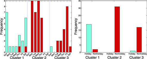
Figure 3: Frequency plots of cluster labels by days of the week (left panel) and by non- and holidays (right panel) for Clusters 1, 2 and 3 (left, middle and right groups).

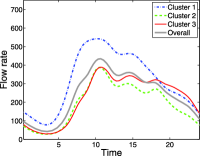
Figure 4: Overall and cluster-specific mean functions of the training data of daily traffic flow rates.

Figure 5: Estimated mean functions (left column) superimposed on the observed trajectories, covariance functions (middle column) and the corresponding eigenfunctions (right column) of Clusters 1–3 (from top to bottom) based on the training data of daily traffic flow trajectories.

The cluster memberships displayed in Figure 3 show that Cluster 1 contains mostly weekends (left panel), with 90% being holidays including weekends (right panel). Cluster 2 completely comprises weekdays including Mondays through Thursdays. Cluster 3 comprises mostly weekdays, especially Fridays (left panel). The mean functions of the three clusters and the overall trajectories are displayed in Figure 4. While Cluster 1 has a higher mean traffic flow rate than the other two clusters, Clusters 2 and 3 have relatively close mean flow rates in terms of shape and magnitude until 11:00, and they diverge thereafter with a higher mean flow rate in Cluster 3. The observed trajectories along with the corresponding covariance functions and leading eigenfunctions are shown in Figure 5. The variability of Cluster 1 is higher than the other two clusters, while Cluster 2 has the lowest variability. The peak flow rate in Cluster 1 lasts from 07:00 to 17:00 and the three leading principal component functions explain 77.16%, 11.14% and 5.57% of total variability. The trajectories in Cluster 2 have a relatively uniform pattern with the major peak flow rate at around 11:00. Cluster 3 indicates a high variability of flow rates occurring after 18:00. The mean integrated prediction errors are defined as ${n_{c}}^{-1}\sum_{i=1}^{n_{c}}{T}^{-1}\int_{0}^{T}(\hat{Z}_{i}^{(c)}(t)-Y_{i}(t))^{2}\,dt$, where $\hat{Z}_{i}^{(c)}(t)=\hat{\mu}^{(c)}(t)+\sum_{j=1}^{M_{c}}\hat{\xi}_{ij}^{(c)}\hat{\varphi}_{j}^{(c)}(t)$, $Y_{i}(t)$ is the observed trajectory and $n_{c}$ is the number of trajectories in Cluster $c$. These are 327.3, 78.8 and 122.4 for Clusters 1–3, respectively. Prediction using the overall trajectories without clustering, in contrast, returned an error of 300.5, indicating that there is a huge reduction in prediction errors when heterogeneity of cluster patterns are taken into account.

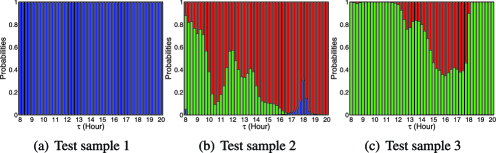
Figure 6: The predicted cluster membership distribution for Clusters 1–3 (indicated in blue, green and red) as a function of the “current time” $\tau$ (per 15 min) for samples from the test data based on the trajectories observed up to $\tau$.

The model fits of the multiclass logistic regression listed in Supplementary Material C [Chiou (2012)] are used in predicting the unobserved trajectory for an up-to-date and partially observed trajectory. Given a newly observed trajectory from the test data up to the current time $\tau$, to consider different flow patterns, we predict the posterior probabilities for each of the associated clusters by functional classification based on the multiclass logistic regression model in (11), using the fitted regression coefficients in (8) with the relative $L^{2}$ distances (10) as the covariate. The posterior probabilities for some test samples are illustrated in Figure 6 with the values of $\tau$ progressing from 08:00 to 20:00 by 15-min intervals. In Figure 6(a), the predicted membership probabilities of Test sample 1 degenerate to one for all values of $\tau$. The associated predicted trajectories are shown in Figure 2(a)–(c). The time-varying prediction intervals, which are wider closer to $\tau$ and taper off toward the end, depend on Cluster 1’s variability pattern as illustrated in Figure 5 (top panels). In contrast, Figure 6(b) for Test sample 2 indicates a more complex situation where the predicted membership distributions change with $\tau$, with the associated predicted trajectories shown in Figure 2(d)–(f). In this case, using the early trajectory information up to $\tau=8\mbox{:}00$ may lead to misclassification, which makes it difficult to predict its future trajectory accurately. This issue is resolved as $\tau$ moves onward. The wider prediction bands with $\tau$ at 12:00 and 16:00, in comparison with that at 8:00, reflect the fact that the variability of Cluster 3’s traffic flow trajectories is larger in the afternoon as illustrated in Figure 5 (bottom panels). Figure 6(c) indicates that the posterior cluster membership probabilities of Test sample 3 alternate between Clusters 2 and 3, owing to certain similarities in these two cluster patterns, and the predicted cluster membership remains with Cluster 3 after around 18:00. Given that the actual cluster memberships are unknown, the accuracy of functional classification for the up-to-date and partially observed trajectories in the test data will be investigated via a simulation study in Section 6.

5 Traffic flow prediction

In predicting the unobserved traffic flow trajectories, we also investigate the effects on the prediction performance of the interval length prior to time $\tau$ and the future interval length after it. To this end, we define ${\mathcal{S}(\tau;\omega)}=[\max(0,\tau-\omega),\tau]$, where $\omega$ is the length of the known interval to be used in prediction calculations and ${\mathcal{T}(\tau;\kappa)}=[\tau,\min(\tau+\kappa,T)]$, where $\kappa$ is the length of the unknown interval to be predicted from time $\tau$ onward. In the test data, given a sample $Y_{i}^{*}$ observed up to time $\tau$, denoted by $Y_{i,{\mathcal{S}(\tau)}}^{*}$, we define the mean integrated prediction error ($\operatorname{MIPE}$) as the the performance measure of predicting $Y_{i,{\mathcal{T}(\tau)}}^{*}$. This is expressed as $\operatorname{MIPE}(\tau,\omega,\kappa)=m_{p}^{-1}\sum_{i=1}^{m_{p}}\kappa^{-1}\int_{0}^{\kappa}\{\widehat{Z}_{i,{\mathcal{T}(\tau)}}^{*}(t)-Y_{i,{\mathcal{T}(\tau)}}^{*}(t)\}^{2}\,dt$, where $Y_{i,{\mathcal{T}(\tau)}}^{*}(t)=Y_{i}^{*}(\tau+t)$, $\widehat{Z}_{i,{\mathcal{T}(\tau)}}^{*}(t)$ is obtained by (18) and $m_{p}$ is the number of trajectories in the test data. For ease of comparisons across different values of $\tau$, let $\tau_{s}=\max(0,\tau-\omega)$ and $\tau_{e}=\min(\tau+\kappa,T)$, for $\omega>0$ and $\kappa>0$. We define the total mean integrated prediction error ($\operatorname{TMIPE}$) for the overall prediction performance by

$$\operatorname{TMIPE}(\omega,\kappa)=\int_{\tau_{s}}^{\tau_{e}}\operatorname{MIPE}(\tau,\omega,\kappa)\,d\tau,$$ (19)

where $\tau_{s}$ and $\tau_{e}$ are the smallest and the largest values, respectively, selected with respect to the times, $\tau$, on the domain $[0,T]$. In this study, $T=24$ (hours) and we set $\tau_{s}=8$ and $\tau_{e}=20$. For notational convenience, we let $\kappa^{*}=24-\tau$ and $\omega^{*}=\tau$, $\tau_{s}\leq\tau\leq\tau_{e}$, such that $\kappa^{*}$ denotes the interval length from the current time to the end of the day and $\omega^{*}$ denotes the maximal length of the past trajectory information available for prediction.

5.1 Results and comparisons of traffic flow prediction

In this study we investigate the prediction performance by comparing the following methods:

• $\mathrm{FP}$: Functional prediction based on functional linear regression using the same setting described in Section 3.1 but without considering clusters of different traffic flow patterns;

• $\mathrm{FMP}_{H}$: Functional prediction using the proposed functional mixture prediction model except that the posterior membership probabilities (6) degenerate to zero or one such that $\sum_{c=1}^{K}P(C=c\mid Z_{\mathcal{S}(\tau)}^{*})=1$ (where the subscript $H$ reflects the so-called hard classification);

• $\mathrm{FMP}_{S}$: Functional prediction using the proposed functional mixture prediction model (where the subscript $S$ reflects the so-called soft classification or probabilistic classification).

Table 2: Performance comparisons for $\mathrm{FP}$, $\mathrm{FMP}_{H}$ and $\mathrm{FMP}_{S}$ based on $\operatorname{TMIPE}$ ($\times 10^{3}$) under various values of $\kappa$ and $\omega$

		$\bolds{\omega}$
	$\bolds{\kappa}$	1	2	3	4	5	6	$\bolds{\omega^{*}}$
$\mathrm{FP}$	1	$4.12$	$4.92$	$4.84$	$4.92$	$5.30$	$5.68$	$5.82$
	4	$7.42$	$7.71$	$7.69$	$8.10$	$8.60$	$9.06$	$8.95$
	8	$9.92$	$10.26$	$10.35$	$10.79$	$11.27$	$11.71$	$11.65$
	$\kappa^{*}$	$12.34$	$12.79$	$12.94$	$13.41$	$13.91$	$14.36$	$14.30$
$\mathrm{FMP}_{H}$	1	$3.48$	$3.22$	$3.20$	$3.33$	$3.53$	$3.52$	$3.14$
(3 clusters)	4	$5.00$	$4.62$	$4.73$	$4.91$	$5.20$	$5.26$	$4.79$
	8	$8.88$	$8.44$	$8.48$	$8.68$	$8.97$	$9.07$	$8.81$
	$\kappa^{*}$	$12.24$	$11.82$	$11.87$	$12.06$	$12.36$	$12.47$	$12.33$
$\mathrm{FMP}_{S}$	1	$3.31$	$3.26$	$3.07$	$2.93$	$2.87$	$2.80$	$2.81$
(3 clusters)	4	$4.37$	$4.14$	$4.05$	$3.98$	$3.80$	$3.86$	$4.18$
	8	$5.80$	$5.64$	$5.54$	$5.49$	$5.41$	$5.61$	$6.68$
	$\kappa^{*}$	$7.97$	$7.94$	$7.84$	$7.86$	$7.71$	$7.89$	$9.95$

Figure 7: Performance comparisons for $\mathrm{FMP}_{S}$, based on $\operatorname{TMIPE}$ (19), displayed as a function of $\kappa$ (left) with $\omega$ fixed at 1, 2, 4 and $\omega^{*}$ and as a function of $\omega$ (right) with $\kappa$ fixed at 1, 4, 7, 10 and $\kappa^{*}$.

To examine prediction performance under various situations, we consider a wide range of values $\tau$ along with various values of $\omega$ and $\kappa$ as defined in ${\mathcal{S}(\tau;\omega)}$ and ${\mathcal{T}(\tau;\kappa)}$. Table 2 indicates that the proposed $\mathrm{FMP}_{S}$ is robust, generally outperforming the other two ($\mathrm{FP}$ and $\mathrm{FMP}_{H}$) under various values of $\omega$ and $\kappa$. Figure 7 (left panel) indicates that small values of $\omega$ $(1,2,4)$ give a similar performance and it is not surprising that the performance for larger values of $\kappa$ is worse. For fixed values of $\kappa$ (right panel), TMIPE as a function of $\omega$ generally shows a positive slope as it moves away from the origin, with a minimum at $\omega=5$ (for $\kappa=4,8,\omega^{*}$) or $\omega=6$ (for $\kappa=1$) from Table 2. The trend is relatively flat, but becomes steeper when $\omega=\omega^{*}$. This discrepancy is more pronounced with increasing $\kappa$. A possible explanation is that the flow trajectory patterns in Clusters 2 and 3 are close in shape and magnitude until noon and diverge thereafter and, thus, using larger $\omega$ with more past information may not significantly improve the overall prediction accuracy. In the literature, Sentürk and Müller (2010) considered the length of past data to be used for prediction and suggested the optimal length using a data-adaptive criterion that minimizes the absolute prediction error. Our empirical results also suggest the use of a data-adaptive criterion to choose the length of past data. Additionally, comparisons for the prediction performance between the methods with fixed values of $\omega$ as illustrated in Figure 8 (with $\omega=1$ on the left and $\omega=\omega^{*}$ on the right) reinforce the conclusion that $\mathrm{FMP}_{S}$ outperforms $\mathrm{FP}$ and $\mathrm{FMP}_{H}$. In addition to the 3-cluster prediction performance illustrated above, results of the 2- and 4-cluster prediction performances are illustrated in Supplementary Material C [Chiou (2012)] for comparisons. These results also support our choice of the 3-cluster model, which outperforms the 2- and 4-cluster models.

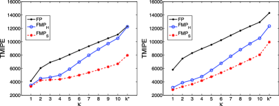
Figure 8: Performance comparisons for $\mathrm{FP}$, $\mathrm{FMP}_{H}$ and $\mathrm{FMP}_{S}$, based on $\operatorname{TMIPE}$ (19), displayed as a function of $\kappa$, with $\omega=1$ (left) and $\omega=\omega^{*}$ (right).

5.2 Comparisons with other methods

We compare the functional mixture prediction approach with an existing method that could also be fitted into our functional mixture prediction framework. One possible approach is to treat the unobserved future trajectory for a partially observed trajectory as missing in the entire trajectory. That is, we may replace (3.3) in Step 3(ii) with the model

$$\hat{Z}^{*(c)}_{\mathcal{T}(\tau)}(t)=\hat{E}\bigl{(}Z^{*}_{\mathcal{T}(\tau)}(t)\mid Y^{*}_{\mathcal{S}(\tau)},C=c\bigr{)}=\hat{\mu}^{*(c)}(t)+\sum_{j=1}^{M_{c}}\hat{\xi}_{j}^{*(c)}\hat{\varphi}_{j}^{*(c)}(t)$$ (20)

for all $t\in{\mathcal{T}(\tau)}$, where the estimated mean function $\hat{\mu}^{*(c)}(t)$ and the estimated eigenfunctions of the covariance kernel $\hat{\varphi}_{j}^{*(c)}(t)$ of cluster $c$ are obtained by the training data set in the clustering step with the corresponding domain ${\mathcal{T}(\tau)}$. The key step is to estimate the functional principal component scores, $\hat{\xi}_{j}^{*(c)}$, which cannot be obtained easily since the trajectory is only partially observed. An existing method that can deal with this situation makes use of the expectation of the posterior distribution in Proposition 1 of Zhou, Serban and Gebraeel (2011), assuming that the prior distribution of the scores is Gaussian, for an application to degradation modeling. This formula coincides with the conditional expectation approach in equation (4) of Yao, Müller and Wang (2005a) under Gaussian assumptions, although they are different in terms of statistical inference. We term this method the Functional Principal Component Prediction (FPCP) approach. We apply FPCP to the proposed functional mixture prediction algorithm including the cases with and without clustering/classification considerations for comparisons, including $\mathrm{FPCP}$, $\mathrm{FPCP}_{H}$ and $\mathrm{FPCP}_{S}$ that are parallel to $\mathrm{FP}$, $\mathrm{FMP}_{H}$ and $\mathrm{FMP}_{S}$. The results shown in Table 3, in comparison with the results in Table 2, indicate that the functional mixture prediction approach in conjunction with functional linear regression outperforms the FPCP approach. Additional results for the 2- and the 4-cluster models are also provided in Supplementary Material C [Chiou (2012)] for comparison.

Table 3: Performance comparisons for $\mathrm{FPCP}$, $\mathrm{FPCP}_{H}$ and $\mathrm{FPCP}_{S}$ based on $\operatorname{TMIPE}$ ($\times 10^{3}$) under various values of $\kappa$ and $\omega$

		$\bolds{\omega}$
	$\bolds{\kappa}$	1	2	3	4	5	6	$\bolds{\omega^{*}}$
$\mathrm{FPCP}$	1	$14.30$	$13.94$	$13.63$	$12.62$	$10.49$	$8.48$	$7.69$
	4	$17.43$	$16.70$	$15.37$	$13.57$	$11.90$	$11.11$	$10.77$
	8	$17.97$	$16.98$	$15.96$	$14.93$	$14.10$	$13.73$	$13.30$
	$\kappa^{*}$	$19.27$	$18.59$	$17.88$	$17.13$	$16.50$	$16.19$	$15.66$
$\mathrm{FPCP}_{H}$	1	$7.83$	$8.62$	$8.90$	$8.90$	$10.57$	$10.67$	$2.85$
(3 clusters)	4	$10.72$	$11.35$	$11.99$	$11.63$	$11.21$	$9.75$	$4.80$
	8	$12.57$	$12.62$	$12.28$	$11.94$	$12.05$	$11.65$	$9.19$
	$\kappa^{*}$	$14.35$	$14.36$	$14.24$	$14.13$	$14.14$	$13.94$	$12.48$
$\mathrm{FPCP}_{S}$	1	$6.26$	$7.29$	$7.54$	$7.73$	$9.41$	$9.44$	$3.07$
(3 clusters)	4	$8.73$	$9.84$	$10.79$	$10.86$	$10.61$	$9.86$	$4.87$
	8	$10.13$	$11.16$	$11.66$	$11.65$	$11.60$	$11.28$	$8.80$
	$\kappa^{*}$	$12.12$	$12.95$	$13.23$	$13.12$	$13.14$	$13.14$	$12.37$

6 Simulation

We implement a Monte Carlo simulation to evaluate the performance of the functional clustering and classification procedures as well as the functional prediction accuracy. We simulate the scenario of the real traffic flow trajectories analyzed in the previous sections. We generate a training data set and a test data set for each simulation run using the estimated results of the 3-cluster traffic flow trajectories as the true models with a total of 100 simulation replicates. The numbers of curves $n_{c}$ are 21, 31 and 18 for Clusters 1–3 in each training data set and are 3, 8 and 3 in each test data as in the previous analysis. The synthetic curves of cluster $c$ are generated by the model $y_{i}^{(c)}(t_{j})=\mu^{(c)}(t_{j})+\sum_{j=1}^{\widetilde{M}_{c}}\xi_{ij}^{(c)}\phi_{j}^{(c)}(t_{j})+\varepsilon_{ij}^{(c)}$, for $i=1,\ldots,n_{c}$, where $\xi_{ij}^{(c)}$ are normal random variates with a mean of zero and variance $\lambda^{(c)}$ and the random measurement errors $\varepsilon_{ij}^{(c)}$ are independent and follow a normal distribution with a mean of zero and variance $\sigma^{2}_{(c)}$. The recording times $t_{j}=j/4$ for $j=1,\ldots,96$ mimic the 15-min recording time interval. The quantities $\mu^{(c)}$, $\phi_{j}^{(c)}$, $\lambda_{j}^{(c)}$ and $\sigma^{2}_{(c)}$ use the model estimates of our real traffic flow data analysis. The numbers of components $\widetilde{M}_{c}$ are determined by the numbers of the estimated $\lambda_{j}^{(c)}$ that are strictly positive. Further details of the simulated models regarding the underlying functions $\mu^{(c)}$ and $\phi_{j}^{(c)}$, along with a sample of synthetic trajectories, are displayed in Supplementary Material D [Chiou (2012)]. The clustering results of this simulated sample, including the estimated mean function and the eigenfunctions along with the covariance functions, are also illustrated.

Table 4: Average $\operatorname{TMIPE}$ ($\times 10^{3}$) (with s.e. in parentheses) for $\mathrm{FP}$, $\mathrm{FMP}_{H}$, $\mathrm{FMP}_{S}$ and $\mathrm{FMP}_{S}^{*}$ under various values of $\kappa$ and $\omega$ based on 100 simulation replicates

		$\bolds{\omega}$
	$\bolds{\kappa}$	1	2	4	6	$\bolds{\omega^{*}}$
$\mathrm{FP}$	1	2.99 (0.03)	3.44 (0.05)	3.90 (0.07)	4.40 (0.08)	4.87 (0.11)
	4	5.53 (0.09)	5.72 (0.10)	6.18 (0.12)	6.70 (0.14)	7.18 (0.17)
	8	6.77 (0.13)	6.92 (0.15)	7.33 (0.17)	7.80 (0.20)	8.26 (0.21)
	$\kappa^{*}$	7.50 (0.18)	7.67 (0.20)	8.08 (0.22)	8.52 (0.24)	8.97 (0.25)
$\mathrm{FMP}_{H}$	1	2.88 (0.04)	3.17 (0.05)	3.42 (0.07)	3.58 (0.08)	3.61 (0.09)
	4	4.98 (0.11)	5.14 (0.12)	5.44 (0.15)	5.65 (0.17)	5.77 (0.18)
	8	6.00 (0.15)	6.12 (0.16)	6.42 (0.19)	6.66 (0.22)	6.89 (0.24)
	$\kappa^{*}$	7.18 (0.27)	7.47 (0.33)	8.02 (0.50)	8.41 (0.57)	8.80 (0.53)
$\mathrm{FMP}_{S}$	1	2.80 (0.04)	3.09 (0.05)	3.30 (0.07)	3.49 (0.07)	3.49 (0.07)
	4	4.88 (0.09)	4.91 (0.10)	5.26 (0.11)	5.44 (0.13)	5.42 (0.13)
	8	5.90 (0.14)	5.99 (0.14)	6.34 (0.16)	6.38 (0.17)	6.59 (0.18)
	$\kappa^{*}$	6.90 (0.19)	7.07 (0.19)	7.25 (0.22)	7.58 (0.23)	7.86 (0.25)
$\mathrm{FMP}_{S}^{*}$	1	2.60 (0.03)	2.81 (0.04)	3.03 (0.05)	3.13 (0.06)	3.13 (0.06)
	4	4.11 (0.06)	4.18 (0.07)	4.40 (0.09)	4.48 (0.10)	4.46 (0.11)
	8	4.57 (0.09)	4.59 (0.09)	4.74 (0.11)	4.78 (0.12)	4.73 (0.13)
	$\kappa^{*}$	4.58 (0.10)	4.57 (0.10)	4.65 (0.12)	4.68 (0.13)	4.62 (0.13)

The average clustering error rates are 6.48% (with standard error 1.28%), 1.68% (0.45%) and 8.39% (2.01%) for Clusters 1–3 based on the 100 simulated training data sets. The accuracy of classification for the future trajectory to be predicted for a partially observed trajectory in the test data depends on the values $\tau$, the “current” time observed thus far. The average classification error rate decreases with $\tau$, ranging from 27.5% at 8:00 to 7.7% at 20:00, implying that prediction accuracy increases with $\tau$. Additional details regarding accuracy of clustering and classification are compiled in Supplementary Material D [Chiou (2012)].

The prediction performances based on the proposed functional mixture prediction (FMP) approach are summarized in Table 4. The method $\mathrm{FMP}_{S}^{*}$ is the same as $\mathrm{FMP}_{S}$, apart from that $\mathrm{FMP}_{S}^{*}$ assumes the cluster/classification memberships are known, serving as the gold standard for prediction performance comparisons. The results clearly demonstrate that $\mathrm{FMP}_{S}$ outperforms $\mathrm{FP}$ and $\mathrm{FMP}_{H}$, with relatively smaller values of TMIPE and the associated standard errors indicating that $\mathrm{FMP}_{S}$ has better prediction accuracy and is quite robust. In $\mathrm{FMP}_{S}$, the prediction errors using $\omega=1$ and $\omega=2$ are close to each other and perform the best under various values of $\kappa$. The optimal selection of $\omega$ appears to be different from those obtained from our real traffic flow data. Although the generated data based on the model estimates may reach a high level of realism to traffic flow data, they may not be able to capture the entire data features such as outlying curves that could influence the prediction performance. In addition, classification errors of the partially observed trajectory may also play a role in prediction. We also compare the FMP method with the FPCP approach. The simulation results are listed in Supplementary Material D [Chiou (2012)]. The results suggest larger values of $\omega$ for minimal prediction errors. The intuition behind these results is that FPCP treats the partial trajectory to be predicted as missing values, especially when the data are more homogeneous within clusters and contain less outlying curves as in the simulated data. Overall, the results demonstrate that the proposed FMP approach outperforms the FPCP approach.

7 Concluding remarks and discussions

This study presents a methodological framework for uncovering traffic flow patterns and predicting traffic flow. The proposed functional data approaches, including classification and prediction, identify clusters with similar traffic flow patterns, facilitating accurate prediction of daily traffic flow. Although motivated by the subject of traffic flow prediction, the proposed methodology is generally applicable and transferable to the analysis and prediction of any longitudinally collected functional data, such as city electricity usage or degradation studies in manufacturing systems. The empirical results demonstrate that our proposed method, functional mixture prediction, which combine functional prediction with probabilistic functional classification, can work reasonably well to predict traffic flow. We conclude that taking traffic flow patterns into account can greatly improve prediction performance as long as the traffic flow patterns can be satisfactorily identified.

In the literature of intelligent transportation systems, conditional expectation is commonly used as the measure of traffic flow prediction/forecast of a future trajectory at a future time point or short period. However, it may be interesting to consider probabilistic forecasts [Gneiting (2008)], which take the form of probability distributions over future trajectories. A probabilistic forecast may engender a new way of thinking about traffic flow prediction, which may give a better account of uncertainty in potential flow trajectories. In this study, our focus was on predicting a future trajectory in the form of conditional expectation for an up-to-date and partially observed trajectory. Under the functional mixture prediction framework, a mixture of predictive distributions of the potential trajectories could instead serve as an ensemble for probabilistic forecasting. However, substantial efforts would be needed to accomplish the goal of probabilistic forecasting for traffic flow trajectories.

In addition to predictive accuracy, the real-time feature of traffic flow information is important in traffic management. Given that the components of our proposed model are estimated based on historical data, as in the training data, the proposed method also serves as a real-time prediction approach for predicting the future unobserved traffic flow trajectory for a partially observed flow trajectory. The fact that real-time information is quickly and easily updated will facilitate the establishment of effective reporting systems for traffic flow prediction. Furthermore, this article discussed single-detector traffic prediction, a category crucial in supporting demand forecasting as required in practice by operational network models. Future research might extend to multiple-detector traffic prediction and will be important in working toward the goal of better road network management.

References

- Abraham et al. (2003) {barticle}[mr] \bauthor\bsnmAbraham, \bfnmC.\binitsC., \bauthor\bsnmCornillon, \bfnmP. A.\binitsP. A., \bauthor\bsnmMatzner-Løber, \bfnmE.\binitsE. and \bauthor\bsnmMolinari, \bfnmN.\binitsN. (\byear2003). \btitleUnsupervised curve clustering using B-splines. \bjournalScand. J. Stat. \bvolume30 \bpages581–595. \biddoi=10.1111/1467-9469.00350, issn=0303-6898, mr=2002229\bptokimsref\endbibitem
- Antoch et al. (2010) {barticle}[mr] \bauthor\bsnmAntoch, \bfnmJaromír\binitsJ., \bauthor\bsnmPrchal, \bfnmLuboš\binitsL., \bauthor\bsnmDe Rosa, \bfnmMaria Rosaria\binitsM. R. and \bauthor\bsnmSarda, \bfnmPascal\binitsP. (\byear2010). \btitleElectricity consumption prediction with functional linear regression using spline estimators. \bjournalJ. Appl. Stat. \bvolume37 \bpages2027–2041. \biddoi=10.1080/02664760903214395, issn=0266-4763, mr=2740138 \bptokimsref \endbibitem
- Aston, Chiou and Evans (2010) {barticle}[mr] \bauthor\bsnmAston, \bfnmJohn A. D.\binitsJ. A. D., \bauthor\bsnmChiou, \bfnmJeng-Min\binitsJ.-M. and \bauthor\bsnmEvans, \bfnmJonathan P.\binitsJ. P. (\byear2010). \btitleLinguistic pitch analysis using functional principal component mixed effect models. \bjournalJ. R. Stat. Soc. Ser. C Appl. Stat. \bvolume59 \bpages297–317. \biddoi=10.1111/j.1467-9876.2009.00689.x, issn=0035-9254, mr=2744475 \bptokimsref \endbibitem
- Bishop and Lasserre (2007) {bincollection}[mr] \bauthor\bsnmBishop, \bfnmChristopher M.\binitsC. M. and \bauthor\bsnmLasserre, \bfnmJulia\binitsJ. (\byear2007). \btitleGenerative or discriminative? Getting the best of both worlds. In \bbooktitleBayesian Statistics 8 \bpages3–24. \bpublisherOxford Univ. Press, \blocationOxford. \bidmr=2433187 \bptnotecheck year\bptokimsref\endbibitem
- Çetiner, Sari and Borat (2010) {barticle}[auto:STB—2012/10/18—06:36:35] \bauthor\bsnmÇetiner, \bfnmB. G.\binitsB. G., \bauthor\bsnmSari, \bfnmM.\binitsM. and \bauthor\bsnmBorat, \bfnmO.\binitsO. (\byear2010). \btitleA neural network based traffic-flow prediction model. \bjournalMath. and Comput. Appl \bvolume15 \bpages269–278. \bptokimsref \endbibitem
- Chen and Grant-Muller (2001) {barticle}[auto:STB—2012/10/18—06:36:35] \bauthor\bsnmChen, \bfnmH.\binitsH. and \bauthor\bsnmGrant-Muller, \bfnmS.\binitsS. (\byear2001). \btitleUse of sequential learning for short-term traffic flow forecasting. \bjournalTransportation Research Part C: Emerging Technologies \bvolume9 \bpages319–336. \bptokimsref \endbibitem
- Chiou (2012) {bmisc}[auto] \bauthor\bsnmChiou, \bfnmJeng-Min\binitsJ.-M. (\byear2012). \bhowpublishedSupplement to “Dynamical functional prediction and classification, with application to traffic flow prediction.” DOI:\doiurl10.1214/12-AOAS595SUPP. \bptokimsref \endbibitem
- Chiou and Li (2007) {barticle}[mr] \bauthor\bsnmChiou, \bfnmJeng-Min\binitsJ.-M. and \bauthor\bsnmLi, \bfnmPai-Ling\binitsP.-L. (\byear2007). \btitleFunctional clustering and identifying substructures of longitudinal data. \bjournalJ. R. Stat. Soc. Ser. B Stat. Methodol. \bvolume69 \bpages679–699. \biddoi=10.1111/j.1467-9868.2007.00605.x, issn=1369-7412, mr=2370075 \bptokimsref \endbibitem
- Chiou and Li (2008) {barticle}[mr] \bauthor\bsnmChiou, \bfnmJeng-Min\binitsJ.-M. and \bauthor\bsnmLi, \bfnmPai-Ling\binitsP.-L. (\byear2008). \btitleCorrelation-based functional clustering via subspace projection. \bjournalJ. Amer. Statist. Assoc. \bvolume103 \bpages1684–1692. \biddoi=10.1198/016214508000000814, issn=0162-1459, mr=2724685 \bptokimsref \endbibitem
- Chiou, Müller and Wang (2003) {barticle}[mr] \bauthor\bsnmChiou, \bfnmJeng-Min\binitsJ.-M., \bauthor\bsnmMüller, \bfnmHans-Georg\binitsH.-G. and \bauthor\bsnmWang, \bfnmJane-Ling\binitsJ.-L. (\byear2003). \btitleFunctional quasi-likelihood regression models with smooth random effects. \bjournalJ. R. Stat. Soc. Ser. B Stat. Methodol. \bvolume65 \bpages405–423. \biddoi=10.1111/1467-9868.00393, issn=1369-7412, mr=1983755 \bptokimsref \endbibitem
- Chiou and Müller (2007) {barticle}[mr] \bauthor\bsnmChiou, \bfnmJeng-Min\binitsJ.-M. and \bauthor\bsnmMüller, \bfnmHans-Georg\binitsH.-G. (\byear2007). \btitleDiagnostics for functional regression via residual processes. \bjournalComput. Statist. Data Anal. \bvolume51 \bpages4849–4863. \biddoi=10.1016/j.csda.2006.07.042, issn=0167-9473, mr=2364544 \bptokimsref \endbibitem
- Chiou and Müller (2009) {barticle}[mr] \bauthor\bsnmChiou, \bfnmJeng-Min\binitsJ.-M. and \bauthor\bsnmMüller, \bfnmHans-Georg\binitsH.-G. (\byear2009). \btitleModeling hazard rates as functional data for the analysis of cohort lifetables and mortality forecasting. \bjournalJ. Amer. Statist. Assoc. \bvolume104 \bpages572–585. \biddoi=10.1198/jasa.2009.0023, issn=0162-1459, mr=2751439 \bptokimsref \endbibitem
- Coffey and Hinde (2011) {barticle}[mr] \bauthor\bsnmCoffey, \bfnmNorma\binitsN. and \bauthor\bsnmHinde, \bfnmJohn\binitsJ. (\byear2011). \btitleAnalyzing time-course microarray data using functional data analysis—a review. \bjournalStat. Appl. Genet. Mol. Biol. \bvolume10 \bpagesArt. 23, 34. \biddoi=10.2202/1544-6115.1671, issn=1544-6115, mr=2800687 \bptokimsref \endbibitem
- Cuevas, Febrero and Fraiman (2007) {barticle}[mr] \bauthor\bsnmCuevas, \bfnmAntonio\binitsA., \bauthor\bsnmFebrero, \bfnmManuel\binitsM. and \bauthor\bsnmFraiman, \bfnmRicardo\binitsR. (\byear2007). \btitleRobust estimation and classification for functional data via projection-based depth notions. \bjournalComput. Statist. \bvolume22 \bpages481–496. \biddoi=10.1007/s00180-007-0053-0, issn=0943-4062, mr=2336349 \bptokimsref \endbibitem
- D’Amato, Piscopo and Russolillo (2011) {barticle}[mr] \bauthor\bsnmD’Amato, \bfnmValeria\binitsV., \bauthor\bsnmPiscopo, \bfnmGabriella\binitsG. and \bauthor\bsnmRussolillo, \bfnmMaria\binitsM. (\byear2011). \btitleThe mortality of the Italian population: Smoothing techniques on the Lee–Carter model. \bjournalAnn. Appl. Stat. \bvolume5 \bpages705–724. \biddoi=10.1214/10-AOAS394, issn=1932-6157, mr=2840172 \bptokimsref \endbibitem
- Dawid (1976) {barticle}[pbm] \bauthor\bsnmDawid, \bfnmA. P.\binitsA. P. (\byear1976). \btitleProperties of diagnostic data distributions. \bjournalBiometrics \bvolume32 \bpages647–658. \bidissn=0006-341X, pmid=963177 \bptokimsref \endbibitem
- Di et al. (2009) {barticle}[mr] \bauthor\bsnmDi, \bfnmChong-Zhi\binitsC.-Z., \bauthor\bsnmCrainiceanu, \bfnmCiprian M.\binitsC. M., \bauthor\bsnmCaffo, \bfnmBrian S.\binitsB. S. and \bauthor\bsnmPunjabi, \bfnmNaresh M.\binitsN. M. (\byear2009). \btitleMultilevel functional principal component analysis. \bjournalAnn. Appl. Stat. \bvolume3 \bpages458–488. \biddoi=10.1214/08-AOAS206, issn=1932-6157, mr=2668715 \bptokimsref \endbibitem
- Fan and Gijbels (1996) {bbook}[mr] \bauthor\bsnmFan, \bfnmJ.\binitsJ. and \bauthor\bsnmGijbels, \bfnmI.\binitsI. (\byear1996). \btitleLocal Polynomial Modelling and Its Applications. \bseriesMonographs on Statistics and Applied Probability \bvolume66. \bpublisherChapman & Hall, \blocationLondon. \bidmr=1383587 \bptokimsref \endbibitem
- Ferraty and Vieu (2006) {bbook}[mr] \bauthor\bsnmFerraty, \bfnmFrédéric\binitsF. and \bauthor\bsnmVieu, \bfnmPhilippe\binitsP. (\byear2006). \btitleNonparametric Functional Data Analysis: Theory and Practice. \bpublisherSpringer, \blocationNew York. \bidmr=2229687 \bptokimsref \endbibitem
- Gao and Niemeier (2008) {barticle}[auto:STB—2012/10/18—06:36:35] \bauthor\bsnmGao, \bfnmH. O.\binitsH. O. and \bauthor\bsnmNiemeier, \bfnmD. A.\binitsD. A. (\byear2008). \btitleUsing functional data analysis of diurnal ozone and NOx cycles to inform transportation emissions control. \bjournalTransportation Research Part D: Transport and Environment \bvolume13 \bpages221–238. \bptokimsref \endbibitem
- Gneiting (2008) {barticle}[mr] \bauthor\bsnmGneiting, \bfnmTilmann\binitsT. (\byear2008). \btitleEditorial: Probabilistic forecasting. \bjournalJ. Roy. Statist. Soc. Ser. A \bvolume171 \bpages319–321. \biddoi=10.1111/j.1467-985X.2007.00522.x, issn=0964-1998, mr=2427336 \bptokimsref \endbibitem
- Hyndman and Shahid Ullah (2007) {barticle}[mr] \bauthor\bsnmHyndman, \bfnmRob J.\binitsR. J. and \bauthor\bsnmShahid Ullah, \bfnmMd.\binitsM. (\byear2007). \btitleRobust forecasting of mortality and fertility rates: A functional data approach. \bjournalComput. Statist. Data Anal. \bvolume51 \bpages4942–4956. \biddoi=10.1016/j.csda.2006.07.028, issn=0167-9473, mr=2364551 \bptokimsref \endbibitem
- James and Sugar (2003) {barticle}[mr] \bauthor\bsnmJames, \bfnmGareth M.\binitsG. M. and \bauthor\bsnmSugar, \bfnmCatherine A.\binitsC. A. (\byear2003). \btitleClustering for sparsely sampled functional data. \bjournalJ. Amer. Statist. Assoc. \bvolume98 \bpages397–408. \biddoi=10.1198/016214503000189, issn=0162-1459, mr=1995716 \bptokimsref \endbibitem
- Kamarianakis, Shen and Wynter (2012) {barticle}[auto:STB—2012/10/18—06:36:35] \bauthor\bsnmKamarianakis, \bfnmY.\binitsY., \bauthor\bsnmShen, \bfnmW.\binitsW. and \bauthor\bsnmWynter, \bfnmL.\binitsL. (\byear2012). \btitleReal-time road traffic forecasting using regime-switching space–time models and adaptive LASSO (with discussion). \bjournalAppl. Stoch. Models Bus. Ind. \bvolume28 \bpages297–323. \bptokimsref \endbibitem
- Kirby, Waston and Dougherty (1997) {barticle}[auto:STB—2012/10/18—06:36:35] \bauthor\bsnmKirby, \bfnmH. R.\binitsH. R., \bauthor\bsnmWaston, \bfnmS. M.\binitsS. M. and \bauthor\bsnmDougherty, \bfnmM. S.\binitsM. S. (\byear1997). \btitleShould we use neural networks or statistical models for short-term motorway traffic forecasting? \bjournalInt. J. Forecasting \bvolume13 \bpages43–50. \bptokimsref \endbibitem
- Li and Chiou (2011) {barticle}[mr] \bauthor\bsnmLi, \bfnmPai-Ling\binitsP.-L. and \bauthor\bsnmChiou, \bfnmJeng-Min\binitsJ.-M. (\byear2011). \btitleIdentifying cluster number for subspace projected functional data clustering. \bjournalComput. Statist. Data Anal. \bvolume55 \bpages2090–2103. \biddoi=10.1016/j.csda.2011.01.001, issn=0167-9473, mr=2785116 \bptokimsref \endbibitem
- López-Pintado and Romo (2006) {bincollection}[mr] \bauthor\bsnmLópez-Pintado, \bfnmSara\binitsS. and \bauthor\bsnmRomo, \bfnmJuan\binitsJ. (\byear2006). \btitleDepth-based classification for functional data. In \bbooktitleData Depth: Robust Multivariate Analysis, Computational Geometry and Applications (\beditor\binitsR. \bsnmLiu, \beditor\binitsR. \bsnmSerfling and \beditor\binitsD. L. \bsnmSouvaine, eds.). \bseriesDIMACS Ser. Discrete Math. Theoret. Comput. Sci. \bvolume72 \bpages103–119. \bpublisherAmer. Math. Soc., \blocationProvidence, RI. \bidmr=2343116 \bptokimsref \endbibitem
- Ma and Zhong (2008) {barticle}[mr] \bauthor\bsnmMa, \bfnmPing\binitsP. and \bauthor\bsnmZhong, \bfnmWenxuan\binitsW. (\byear2008). \btitlePenalized clustering of large-scale functional data with multiple covariates. \bjournalJ. Amer. Statist. Assoc. \bvolume103 \bpages625–636. \biddoi=10.1198/016214508000000247, issn=0162-1459, mr=2435467 \bptokimsref \endbibitem
- McCullagh and Nelder (1983) {bbook}[mr] \bauthor\bsnmMcCullagh, \bfnmP.\binitsP. and \bauthor\bsnmNelder, \bfnmJ. A.\binitsJ. A. (\byear1983). \btitleGeneralized Linear Models. \bpublisherChapman & Hall, \blocationLondon. \bidmr=0727836 \bptnotecheck year\bptokimsref \endbibitem
- Müller (2005) {barticle}[mr] \bauthor\bsnmMüller, \bfnmHans-Georg\binitsH.-G. (\byear2005). \btitleFunctional modelling and classification of longitudinal data. \bjournalScand. J. Stat. \bvolume32 \bpages223–246. \biddoi=10.1111/j.1467-9469.2005.00429.x, issn=0303-6898, mr=2188671 \bptokimsref \endbibitem
- Müller (2009) {bincollection}[mr] \bauthor\bsnmMüller, \bfnmHans-Georg\binitsH.-G. (\byear2009). \btitleFunctional modeling of longitudinal data. In \bbooktitleLongitudinal Data Analysis (\beditor\binitsG. \bsnmFitzmaurice, \beditor\binitsM. \bsnmDavidian, \beditor\binitsG. \bsnmVerbeke and \beditor\binitsG. \bsnmMolenberghs, eds.) \bpages223–251. \bpublisherCRC Press, \blocationBoca Raton, FL. \bidmr=1500120 \bptnotecheck year\bptokimsref \endbibitem
- Müller, Chiou and Leng (2008) {barticle}[pbm] \bauthor\bsnmMüller, \bfnmHans-Georg\binitsH.-G., \bauthor\bsnmChiou, \bfnmJeng-Min\binitsJ.-M. and \bauthor\bsnmLeng, \bfnmXiaoyan\binitsX. (\byear2008). \btitleInferring gene expression dynamics via functional regression analysis. \bjournalBMC Bioinformatics \bvolume9 \bpages60. \biddoi=10.1186/1471-2105-9-60, issn=1471-2105, pii=1471-2105-9-60, pmcid=2335302, pmid=18226220 \bptokimsref \endbibitem
- Müller and Zhang (2005) {barticle}[mr] \bauthor\bsnmMüller, \bfnmHans-Georg\binitsH.-G. and \bauthor\bsnmZhang, \bfnmYing\binitsY. (\byear2005). \btitleTime-varying functional regression for predicting remaining lifetime distributions from longitudinal trajectories. \bjournalBiometrics \bvolume61 \bpages1064–1075. \biddoi=10.1111/j.1541-0420.2005.00378.x, issn=0006-341X, mr=2216200 \bptokimsref \endbibitem
- Ng and Jordan (2002) {barticle}[auto:STB—2012/10/18—06:36:35] \bauthor\bsnmNg, \bfnmA. Y.\binitsA. Y. and \bauthor\bsnmJordan, \bfnmM. I.\binitsM. I. (\byear2002). \btitleOn discriminative vs. generative classifier: A comparison of logistic regression and naive Bayes. \bjournalNeural Information Processing System \bvolume2 \bpages841–848. \bptokimsref \endbibitem
- Okutani and Stephanides (1984) {barticle}[auto:STB—2012/10/18—06:36:35] \bauthor\bsnmOkutani, \bfnmI.\binitsI. and \bauthor\bsnmStephanides, \bfnmY. J.\binitsY. J. (\byear1984). \btitleDynamic prediction of traffic volume through Kalman filtering theory. \bjournalTransportation Research Part B: Methodological \bvolume18 \bpages1–11. \bptokimsref \endbibitem
- Ramsay and Dalzell (1991) {barticle}[mr] \bauthor\bsnmRamsay, \bfnmJ. O.\binitsJ. O. and \bauthor\bsnmDalzell, \bfnmC. J.\binitsC. J. (\byear1991). \btitleSome tools for functional data analysis. \bjournalJ. Roy. Statist. Soc. Ser. B \bvolume53 \bpages539–572. \bidissn=0035-9246, mr=1125714 \bptnotecheck related\bptokimsref \endbibitem
- Ramsay and Silverman (2002) {bbook}[mr] \bauthor\bsnmRamsay, \bfnmJ. O.\binitsJ. O. and \bauthor\bsnmSilverman, \bfnmB. W.\binitsB. W. (\byear2002). \btitleApplied Functional Data Analysis: Methods and Case Studies. \bpublisherSpringer, \blocationNew York. \biddoi=10.1007/b98886, mr=1910407 \bptokimsref \endbibitem
- Ramsay and Silverman (2005) {bbook}[mr] \bauthor\bsnmRamsay, \bfnmJ. O.\binitsJ. O. and \bauthor\bsnmSilverman, \bfnmB. W.\binitsB. W. (\byear2005). \btitleFunctional Data Analysis, \bedition2nd ed. \bpublisherSpringer, \blocationNew York. \bidmr=2168993 \bptokimsref \endbibitem
- Rice (2004) {barticle}[mr] \bauthor\bsnmRice, \bfnmJohn A.\binitsJ. A. (\byear2004). \btitleFunctional and longitudinal data analysis: Perspectives on smoothing. \bjournalStatist. Sinica \bvolume14 \bpages631–647. \bidissn=1017-0405, mr=2087966 \bptokimsref \endbibitem
- Sentürk and Müller (2010) {barticle}[auto] \bauthor\bsnmSentürk, \bfnmD.\binitsD. and \bauthor\bsnmMüller, \bfnmH.-G.\binitsH.-G. (\byear2010). \btitleFunctional varying coefficient models for longitudinal data. \bjournalJ. Amer. Statist. Assoc. \bvolume105 \bpages1256–1264. \bptokimsref \endbibitem
- Serban and Wasserman (2005) {barticle}[mr] \bauthor\bsnmSerban, \bfnmNicoleta\binitsN. and \bauthor\bsnmWasserman, \bfnmLarry\binitsL. (\byear2005). \btitleCATS: Clustering after transformation and smoothing. \bjournalJ. Amer. Statist. Assoc. \bvolume100 \bpages990–999. \biddoi=10.1198/016214504000001574, issn=0162-1459, mr=2201025 \bptokimsref \endbibitem
- Smith and Demetsky (1997) {barticle}[auto:STB—2012/10/18—06:36:35] \bauthor\bsnmSmith, \bfnmB. L.\binitsB. L. and \bauthor\bsnmDemetsky, \bfnmM. J.\binitsM. J. (\byear1997). \btitleShort-term traffic flow prediction: Neural network approach. \bjournalTransportation Research Record: Journal of the Transportation Research Board \bvolume1453 \bpages98–104. \bptokimsref \endbibitem
- Smith, William and Oswald (2002) {barticle}[auto:STB—2012/10/18—06:36:35] \bauthor\bsnmSmith, \bfnmB. L.\binitsB. L., \bauthor\bsnmWilliam, \bfnmB. M.\binitsB. M. and \bauthor\bsnmOswald, \bfnmR. K.\binitsR. K. (\byear2002). \btitleComparison of parametric and nonparametric models for traffic flow forecasting. \bjournalTransportation Research Part C: Emerging Technologies \bvolume10 \bpages303–321. \bptokimsref \endbibitem
- Stathopoulos and Karlaftis (2003) {barticle}[auto:STB—2012/10/18—06:36:35] \bauthor\bsnmStathopoulos, \bfnmA.\binitsA. and \bauthor\bsnmKarlaftis, \bfnmM. G.\binitsM. G. (\byear2003). \btitleA multivariate state space approach for urban traffic flow modeling and prediction. \bjournalTransportation Research Part C: Emerging Technologies \bvolume11 \bpages121–135. \bptokimsref \endbibitem
- Sun et al. (2003) {barticle}[auto:STB—2012/10/18—06:36:35] \bauthor\bsnmSun, \bfnmH.\binitsH., \bauthor\bsnmLiu, \bfnmH. X.\binitsH. X., \bauthor\bsnmXiao, \bfnmH.\binitsH., \bauthor\bsnmHe, \bfnmR. R.\binitsR. R. and \bauthor\bsnmRan, \bfnmB.\binitsB. (\byear2003). \btitleUse of local linear regression model for short-term traffic forecasting. \bjournalTransportation Research Record \bvolume1836 \bpages143–150. \bptokimsref \endbibitem
- Vlahogianni, Karlaftis and Golias (2008) {barticle}[auto:STB—2012/10/18—06:36:35] \bauthor\bsnmVlahogianni, \bfnmE. I.\binitsE. I., \bauthor\bsnmKarlaftis, \bfnmM. G.\binitsM. G. and \bauthor\bsnmGolias, \bfnmJ. C.\binitsJ. C. (\byear2008). \btitleTemporal evolution of short-term urban traffic flow: A nonlinear dynamic approach. \bjournalComputer-Aided Civil and Infrastructure Engineering \bvolume22 \bpages326–334. \bptokimsref \endbibitem
- Williams and Hoel (2003) {barticle}[auto:STB—2012/10/18—06:36:35] \bauthor\bsnmWilliams, \bfnmB. M.\binitsB. M. and \bauthor\bsnmHoel, \bfnmL. A.\binitsL. A. (\byear2003). \btitleModeling and forecasting vehicular traffic flow as a seasonal ARIMA process: Theoretical basis and empirical results. \bjournalJournal of Transportation Engineering \bvolume129 \bpages664–672. \bptokimsref \endbibitem
- Xie, Zhang and Ye (2007) {barticle}[auto:STB—2012/10/18—06:36:35] \bauthor\bsnmXie, \bfnmY.\binitsY., \bauthor\bsnmZhang, \bfnmY.\binitsY. and \bauthor\bsnmYe, \bfnmZ.\binitsZ. (\byear2007). \btitleShort-term traffic volume forecasting using Kalman filter with discrete wavelet decomposition. \bjournalComputer-Aided Civil and Infrastructure Engineering \bvolume22 \bpages326–334. \bptokimsref \endbibitem
- Xue and Titterington (2008) {barticle}[auto:STB—2012/10/18—06:36:35] \bauthor\bsnmXue, \bfnmJ. H.\binitsJ. H. and \bauthor\bsnmTitterington, \bfnmD. M.\binitsD. M. (\byear2008). \btitleComment on “On discriminative vs. generative classifier: A comparison of logistic regression and naive Bayes.” \bjournalNeural Process Letters \bvolume28 \bpages169–187. \bptokimsref \endbibitem
- Yao, Müller and Wang (2005a) {barticle}[mr] \bauthor\bsnmYao, \bfnmFang\binitsF., \bauthor\bsnmMüller, \bfnmHans-Georg\binitsH.-G. and \bauthor\bsnmWang, \bfnmJane-Ling\binitsJ.-L. (\byear2005a). \btitleFunctional data analysis for sparse longitudinal data. \bjournalJ. Amer. Statist. Assoc. \bvolume100 \bpages577–590. \biddoi=10.1198/016214504000001745, issn=0162-1459, mr=2160561 \bptokimsref \endbibitem
- Yao, Müller and Wang (2005b) {barticle}[mr] \bauthor\bsnmYao, \bfnmFang\binitsF., \bauthor\bsnmMüller, \bfnmHans-Georg\binitsH.-G. and \bauthor\bsnmWang, \bfnmJane-Ling\binitsJ.-L. (\byear2005b). \btitleFunctional linear regression analysis for longitudinal data. \bjournalAnn. Statist. \bvolume33 \bpages2873–2903. \biddoi=10.1214/009053605000000660, issn=0090-5364, mr=2253106 \bptokimsref \endbibitem
- Yin et al. (2002) {barticle}[auto:STB—2012/10/18—06:36:35] \bauthor\bsnmYin, \bfnmH.\binitsH., \bauthor\bsnmWong, \bfnmS. C.\binitsS. C., \bauthor\bsnmXu, \bfnmJ.\binitsJ. and \bauthor\bsnmWong, \bfnmC. K.\binitsC. K. (\byear2002). \btitleUrban traffic flow prediction using fuzzy-neural approach. \bjournalTransportation Research Part C: Emerging Technologies \bvolume10 \bpages85–98. \bptokimsref \endbibitem
- Zhang and Ye (2008) {barticle}[auto:STB—2012/10/18—06:36:35] \bauthor\bsnmZhang, \bfnmY.\binitsY. and \bauthor\bsnmYe, \bfnmZ.\binitsZ. (\byear2008). \btitleShort-term traffic flow forecasting using fuzzy logic system methods. \bjournalJournal of Intelligent Transportation System \bvolume12 \bpages102–112. \bptokimsref \endbibitem
- Zhao, Marron and Wells (2004) {barticle}[mr] \bauthor\bsnmZhao, \bfnmXin\binitsX., \bauthor\bsnmMarron, \bfnmJ. S.\binitsJ. S. and \bauthor\bsnmWells, \bfnmMartin T.\binitsM. T. (\byear2004). \btitleThe functional data analysis view of longitudinal data. \bjournalStatist. Sinica \bvolume14 \bpages789–808. \bidissn=1017-0405, mr=2087973 \bptokimsref \endbibitem
- Zheng, Lee and Shi (2006) {barticle}[auto:STB—2012/10/18—06:36:35] \bauthor\bsnmZheng, \bfnmW.\binitsW., \bauthor\bsnmLee, \bfnmD. H.\binitsD. H. and \bauthor\bsnmShi, \bfnmQ.\binitsQ. (\byear2006). \btitleShort-term freeway traffic prediction: Bayesian combined neural network approach. \bjournalJournal of Transportation Engineering \bvolume132 \bpages114–121. \bptokimsref \endbibitem
- Zhou, Serban and Gebraeel (2011) {barticle}[mr] \bauthor\bsnmZhou, \bfnmRensheng R.\binitsR. R., \bauthor\bsnmSerban, \bfnmNicoleta\binitsN. and \bauthor\bsnmGebraeel, \bfnmNagi\binitsN. (\byear2011). \btitleDegradation modeling applied to residual lifetime prediction using functional data analysis. \bjournalAnn. Appl. Stat. \bvolume5 \bpages1586–1610. \biddoi=10.1214/10-AOAS448, issn=1932-6157, mr=2849787 \bptokimsref \endbibitem