Australia Telescope Compact Array observations of Fermi unassociated sources

Abstract

We report results of the first phase of observations with the Australia Telescope Compact Array (ATCA) at 5 and 9 GHz of the fields around 411 $\gamma$-ray sources with declinations $<+10\degr$ detected by Fermi but marked as unassociated in the 2FGL catalogue. We have detected 424 sources with flux densities in a range of 2 mJy to 6 Jy that lie within the 99 per cent localisation uncertainty of 283 $\gamma$-ray sources. Of these, 146 objects were detected in both the 5 and 9 GHz bands. We found 84 sources in our sample with a spectral index flatter than -0.5. The majority of detected sources are weaker than 100 mJy and for this reason were not found in previous surveys. Approximately 1/3 of our sample, 128 objects, have the probability of being associated by more than 10 times than the probability of being a background source found in the vicinity of a $\gamma$-ray object by chance. We present the catalogue of positions of these sources, estimates of their flux densities and spectral indices where available.

1 Introduction

Analysis of the first two years of Fermi/LAT observations yielded a catalogue of 1872 $\gamma$-ray sources (Nolan et al., 2012, hereafter 2FGL). Of these, 70 per cent have associations with blazars, pulsars, supernova remnants or other objects. The procedure for assigning associations is described in full detail in Ackermann et al. (2012). However, the 2FGL catalogue still does not provide associations for 573 $\gamma$-ray sources. The positional accuracy of Fermi ranges from 0.1 arcmin to 16.6 arcmin with a median $1\sigma$ uncertainty of 2.0 arcmin. These large position errors prevent finding associations by direct matching the 2FGL against optical or infrared catalogues.

Previous analysis of the 1FGL catalogue (Kovalev, 2009) has confirmed earlier EGRET results: that $\gamma$-ray emission and parsec-scale radio emission are strongly related. Extending this study to the 2FGL catalogue, we found that 770 out of 1872 Fermi sources, roughly one half, have been detected in VLBI surveys at 8 GHz (as of December 2012). All these objects are Active Galactic Nuclei (AGN). This is the dominant population of point-like Fermi sources outside of the Galactic plane. Other types of objects associated with $\gamma$-ray sources are supernova remnants, novae, pulsar wind nebulae, x-ray binaries, microquasars, and pulsars. Unassociated sources may belong to any of these classes or may, in part, constitute an as-yet-unknown population. Due to the correlation of $\gamma$-ray emission with parsec-scale radio emission, high resolution radio observations are useful for classification of unassociated $\gamma$-ray sources. Supernova remnants and pulsar wind nebulae are extended objects and, as such, high resolution radio interferometric observations tend to resolve out their emission making them undetectable. Pulsars are generally weak at high frequencies ($>5$ GHz) as they generally have steep spectral indices. Therefore, sources detected with VLBI that are brighter than 1 mJy are almost always AGNs. Detection of a radio bright AGN within the Fermi position error ellipse presents a strong argument that this is likely the same object. Therefore, systematic high resolution radio observations of unassociated Fermi objects promise to find all $\gamma$-ray sources associated with radio-loud AGNs and shrink the list of objects that remain unassociated with an astrophysical source.

It was shown by Lister et al. (2009) and Kovalev (2009) that $\gamma$-ray fluxes and 8 GHz radio flux densities from regions smaller than 5 mas are correlated. Source variability confirms that both radio and $\gamma$-ray emission comes from parsec-scale regions. Therefore, a flux-limited sample of $\gamma$-ray AGNs, such as 2FGL, should be contained within a flux-limited sample of compact radio sources. Compact radio sources from a flux-limited catalogue found within the position error ellipses of sources from a $\gamma$-ray flux limited catalogue can be considered with a high confidence as the same objects, provided that the probability of finding a background radio-loud source within the error ellipse is small. As the search area becomes smaller, weaker radio-loud AGNs can be associated with a $\gamma$-ray source.

In order to evaluate the probability of finding a background source in a given search area, we investigated the cumulative all-sky catalogue of compact radio sources detected with VLBI in the absolute astrometry mode (Petrov and Kovalev, in preparation). This catalogue, as of December 2012, had 7215 objects detected in numerous VLBI surveys over the last several decades: Very Long Baseline Array (VLBA) Calibrator Survey (Beasley et al., 2002; Fomalont et al., 2003; Petrov et al., 2005, 2006; Kovalev et al., 2007; Petrov et al., 2008), Long Baseline Array (LBA) calibrator survey (Petrov et al., 2011b), VLBA Galactic Plane Survey (Petrov et al., 2011a), European VLBI Network (EVN) Galactic plane survey (Petrov, 2012), VLBA imaging and polarimetry survey (Taylor et al., 2007; Petrov & Taylor, 2011), regular VLBA geodetic observations (Petrov et al., 2009; Pushkarev & Kovalev, 2012), and ongoing VLBI observations of 2MASS galaxies (Condon et al., 2011). Figure 1 shows the dependence of the logarithm of the number of sources in the whole sky $N$ with a flux density greater than $S$, as a function of the logarithm of $S$ determined as the median correlated flux density at baseline projection lengths in a range of 100–900 km at 8 GHz. We see that the dependence can be approximated as $N(S)\approx 327\cdot S^{-1.237}$ in a range of [0.18, 5] Jy. We interpret the deviation of $\log N(\log S)$ from the straight line below 180 mJy as evidence of incompleteness. Assuming the parent population remains the same for sources as weak as 1 mJy, we can extrapolate the number of compact sources in the celestial sphere derived for the range [0.18, 5] Jy to the range [1, 180] mJy.

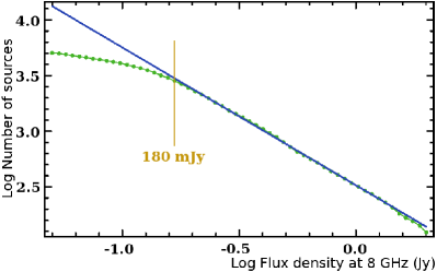
Figure 1: Dependence of the decimal logarithm of the number of compact sources versus the decimal logarithm of their minimum correlated flux density from regions smaller than 50 mas at 8 GHz.

Let us consider a search for a radio counterpart within the area where the probability of source localisation is $P$. Then, assuming localisation errors follow the 2D normal distribution with the second moment $\sigma$, the mathematical expectation of the number of background sources that can be found in that area is

$$M(\sigma,S,P)=-\frac{\displaystyle\sigma^{2}}{\displaystyle 2\pi}\,\ln(1-P)\,N(S).$$ (1)

The function $M(\sigma,S)$ depends on both the position uncertainty, the flux density, and the probability of localisation. When $M\ll 1$, it can be interpreted as the probability of at least one source being found within the area of position uncertainty. If we fix $M(\sigma,S)$ to a specific value, for instance, 0.1, and fix localisation probability, e.g. to 0.95, we can find the dependence of the maximum flux density $S$ of a background source that can be found within the area of localisation with a certain probability (10 per cent in our example) on the standard deviation of localisation. This dependence is shown in Figure 2. For the median 1$\sigma$ position uncertainty of unassociated sources from the 2FGL catalogue 3.0 arcmin, the probability to find a background source brighter than 10.9 mJy is 10 per cent. For 80 per cent of 2FGL source, $1\sigma$ position uncertainty is less than 4.0 arcmin. The flux density that corresponds to 10 per cent probability to find a background source with such a position uncertainty is 17.3 mJy.

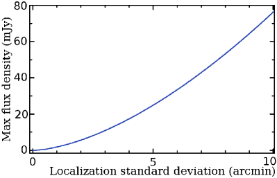
Figure 2: Maximum flux density at 8 GHz of a background compact source to be found with the probability of 10 per cent within an error ellipse with a given $1\sigma$ standard deviation.

In order to check the validity of the reported 2FGL position uncertainties, we computed arcs between 770 $\gamma$-ray objects that have counterparts with radio sources observed with VLBI, and normalised them to their standard deviations derived from parameters of their 2FGL error ellipses:

$$n=\sqrt{\Delta^{2}\alpha\cos^{2}\delta+\Delta^{2}\delta}\>\frac{\displaystyle\sqrt{\sigma^{2}_{\rm maj}\sin^{2}\beta+\sigma^{2}_{\rm min}\cos^{2}\beta}}{\displaystyle\sigma_{\rm maj}\,\sigma_{\rm min}},$$ (2)

where angle $\beta$ is

$$\beta=\arctan{\frac{\displaystyle\Delta\delta}{\displaystyle\Delta\alpha\,\cos\delta}-(\pi/2-\theta)}$$ (3)

and $\sigma_{\rm maj}$, $\sigma_{\rm min}$, and $\theta$ are semi-major, semi-minor axes and position angle of the 2D Normal distribution that describes errors of source localisation. We derived $\sigma_{\rm maj}$, $\sigma_{\rm min}$ from the so-called “95% confidence source semi-major and semi-minor axes” reported in table 3 of the 2FGL catalogue by scaling them by 1/e. The distribution of normalised arcs between the VLBI and 2FGL positions follows a Rayleigh distribution with $\sigma=1$ very closely (Figure 3). The histogram is best fit into a Rayleigh distribution with $\sigma=1.026$. Since VLBI positions are five orders of magnitude more accurate than the positions reported in 2FGL, they are considered as true. We conclude that the 2FGL position errors are realistic and can be used for a probabilistic inference.

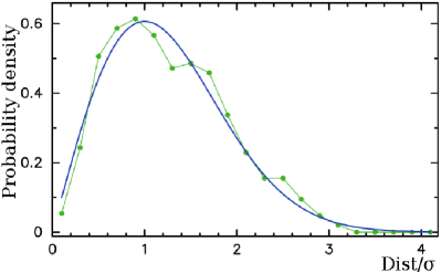
Figure 3: Distribution of position offsets normalised by their standard deviations between 770 Fermi sources and their counterparts detected with VLBI. The solid blue lines shows Rayleigh distribution with $\sigma=1$.

These estimates show that radio observations are an efficient way to identify AGNs associated with $\gamma$-ray sources. According to our experience, it is not difficult to detect sources with flux densities of several mJy using radio interferometers. As we have shown in Figure 1, the cumulative catalogue of compact radio sources detected with VLBI is complete only to the level of 180 mJy. Sources with correlated flux densities between 2 and 180 mJy may not have been marked as associations with 2FGL objects because they were missing from VLBI surveys. However, not all associations of $\gamma$-ray sources in 2FGL are made on the basis of VLBI observations. In the absence of VLBI observations, the source spectrum can be used as a proxy. It was found a long time ago (Kellermann & Pauliny-Toth, 1969) that sources with a spectral index flatter than $-0.5$ tend to be compact as they are dominated by emission from the core. The problem is that existing catalogues are not complete enough to determine the spectrum in the range of flux densities from 1–100 mJy, especially in the southern hemisphere.

These considerations prompted us to propose a program of observations of all unassociated 2FGL sources. The eventual goal of the program is to find all AGNs with correlated flux densities brighter than 2 mJy at 8 GHz from regions smaller than 50 mas within the areas of 99 per cent probability of Fermi localisation uncertainties. Association with a VLBI source automatically improves positions of $\gamma$-ray objects from arcminutes to milliarcseconds, allowing for an unambiguous association with sources at other wavelengths, for instance, optical. Combined with results of on-going programs to find pulsars associated with Fermi sources, for instance Barr et al. (2013), we expect the list of unassociated sources to shrink. At the moment we do not know whether the list will shrink to zero or a population of radio-quiet $\gamma$-ray sources will be found.

In this paper we report early results of the first step of the program of observations of Fermi unassociated sources: observations with the Australia Telescope Compact Array (ATCA) of 411 sources with $\delta<+10\degr$. A brief overview of the program is given in section 2. The data analysis procedure is described in section 3. Results, the catalogue of 375 potential associations for 2FGL sources is given in section  4 followed by concluding remarks.

2 Observations

2.1 Observing Program

The areas of 99 per cent probability of 2FGL localisation, which corresponds to $3.035\sigma$, are typically 4–6 arcmin. They are still too large for a blind search with VLBI using traditional approaches. Therefore, we organised observations in several stages. In the first stage we observed the sources with connected interferometers, the Very Large Array (VLA) in the northern hemisphere, and ATCA in the southern hemisphere. Observations are made in the remote wings of the wide-band receiving system that covers 4.5–10.0 GHz. The sky distribution of target sources is presented in Figure 4.

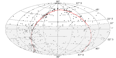
Figure 4: The distribution of 573 2FGL unassociated sources. The area of this survey is shown with grey colour.

We split the source list into two parts. A list of 411 sources with declinations lower than $+10\degr$ was observed with the ATCA. A list of 215 sources with declinations higher than $0\degr$ was observed with the VLA. This list includes 35 overlapping sources in the declination band $[0,+10\degr]$ and 18 sources tentatively associated with supernova remnants and pulsar wind nebulae. Results of the VLA observations will be reported in a separate paper (F. Schinzel et al., (2013) in preparation).

Observations at two frequencies allow us to determine spectral indices. The spectral index is defined as $S\sim f^{\alpha}$, where $S$ is the flux density, and $f$ is the frequency. Sources with a spectral index $\alpha$ greater than $-0.5$ are classified as flat spectrum sources and are therefore considered as likely associations. Bright detected sources will be followed up with the VLBA and LBA. Detection of emission at parsec scales will firmly associate them with the compact core regions of AGNs.

2.2 ATCA observations

We observed a list of 411 target sources with ATCA on September 19–20 2012 for 29 hours. We used the automatic scheduling software sur_sked originally developed for VLBI survey experiments (Petrov et al., 2011b). In order to maximise the observing efficiency, we reduced the correlator cycle time from the usual 10 seconds to 6 seconds, and observed in the mosaic mode to minimise correlator overheads when changing sources. We tried to observe each target source in three scans of 24 seconds each, separated by at least three hours in a sequence that minimises slewing time. In fact, we observed 80 sources in 4 scans, 239 sources in 3 scans and 92 sources in 2 scans. At the beginning of the experiment we observed the primary amplitude calibrator 1934$-$638 for 20 minutes. The automatic scheduling process checked that for every target source a phase calibrator was inserted into the schedule that satisfied two criteria: that the arc between the target and the calibrator should be less than $20\degr$ and a calibrator should be observed within 20 minutes of the target. We used a pool of 1464 compact sources with $\delta<+20\degr$ and correlated flux densities $>200$ mJy. The scheduling process picked up 207 sources from this pool. Many adjacent target scans reused the same phase calibrator. Each calibrator scan was observed for 18 seconds.

The array was in the H214 hybrid configuration with baselines ranging from 31–214 meters between the inner 5 antennas and $\sim$4.4 km between CA06 and the inner antennas. We observed simultaneously in two bands, both 2GHz wide, centred on 5.5 and 9.0 GHz. During data reduction the band edges were excluded and the ranges [4.58, 6.42] GHz (hereafter 5 GHz band) and [8.09, 9.92] GHz (hereafter 9 GHz band) were used. The data were recorded in both polarizations with the Compact Array Broadband Backend (Wilson et al., 2011).

3 Data Analysis

The ATCA correlator provided us the output with frequency resolution 1 MHz and time resolution 6 s. We used the software package Miriad (Sault, Teuben & Wright, 1995) for development of the analysis pipeline. The data processing carried out the following steps:

1. We split the data into subbands and into scans. We discarded data from the remote CA06 station for imaging analysis.

2. We analysed the observations of all the sources and flagged the data affected by radio interference using the task pgflag.

3. We used the Miriad task mfcal for the bandpass solution, using the data of 1934$-$638 with a solution interval of 2 minutes. This bandpass was applied to all the data.

4. We determined the antenna gains and polarization leakage of phase calibrators using the Miriad task gpcal and we also corrected the flux scale with the task gpboot. The complex gain factors were then applied to the target sources.

5. All calibrated visibilities of a target source were merged into one file. The visibilities were inverted using the Miriad task invert using the multi-frequency synthesis algorithm. The typical image size was $1024\times 1024$ with a pixel size of 2.4 arcsec although for some target sources we changed the pixel size later during the data analysis. We tapered the data according to Brigg’s visibility weighting robustness parameter factor 0.5 during inversion.

6. We cleaned the data using the Miriad task mfclean. The default CLEAN gain was set to 0.01 and the default maximum number of iterations was set to 192. The default clean region was 93 per cent of the image.

7. We searched for point sources in the cleaned image using the task imsad, requiring the flux densities to be greater than 5.5 times the image noise root mean square (rms).

8. We performed the non-linear least square fit for positions and parameters of the Gaussian models of detected sources to calibrated visibilities using the Miriad task uvsfit. This task also computed the spectral index. We used positions and flux densities of all sources found by imsad, excluding those flagged as spurious, as the initial values for the fit to the visibility data. A detailed description of the procedure is given below. We ran this procedure for each subband separately.

9. For sources detected in both subbands we computed spectral indices between 5 GHz and 9 GHz.

The task uvsfit estimates source parameters through the minimisation of the least-squared differences between the measured visibilities and those computed from a model source or sources.

Given a set of observed visibilities, each measured at a point $(u,v)$ that is the projected baseline vector expressed in wavelengths, and at a frequency $f$, we write $V_{i}=V(u_{i},v_{i},f_{i})$. There are $n=n_{b}\times n_{f}$ visibility measurements, where $n_{b}$ and $n_{f}$ are the number of baselines and the number of frequency channels respectively.

Given a model source, we can compute model visibilities $M_{i}=M(u_{i},v_{i},f_{i})$ at each point in $(u,v,f)$ space for which we have visibility measurements. The model visibilities can be calculated as the sum of visibilities for several model sources. The fitting process is the adjustment of model source parameters to minimise the quantity $\sum|V_{i}-M_{i}|^{2}$. Both tasks use the Levenberg-Marquardt algorithm for function minimisation. The diagonal terms of the covariance matrix are returned as the variances in fitted parameter values.

For a point source with flux-density $S$ and position $(l,m)$ relative to the phase centre, uvfit computes each model visibility as: $M(u,v)=S(\cos{\theta}+i\sin{\theta})$, where $\theta=2\pi(ul+vm)$.

In uvsfit, the flux-density is expressed as a function of frequency, and new parameters are introduced to describe the spectral shape. The model source is now a function of $S_{0}$, the flux-density at a reference frequency $f_{0}$, position relative to phase centre $(l,m)$, and spectral shape parameters $(\alpha_{0},\alpha_{1},\alpha_{2})$. The model visibilities are then:

$$\begin{array}[]{l @{\;} l}M(u,v,f)&=S(f)(\cos\theta+i\sin\theta)\\ \theta&=2\pi(ul+vm)\\ S(f)&=S_{0}\left(\frac{\displaystyle f}{\displaystyle f_{0}}\right)^{\alpha}\\ \alpha&=\alpha_{0}+\alpha_{1}(f-f_{0})+\alpha_{2}(f-f_{0})^{2}.\end{array}$$ (8)

Model visibilities for the two-dimensional Gaussian source with flux-density $S(f)$, position $(l,m)$, major and minor axes and position angle $(a,b,\phi)$, and spectral shape described by $(\alpha_{0},\alpha_{1},\alpha_{2})$ are calculated by uvsfit as:

$$\begin{array}[]{l @{\;} l}M(u,v,f)&=S(f)(\cos{\theta}+i\sin{\theta})\exp(-\frac{\pi^{2}}{4\log 2}\beta)\\ \theta&=2\pi(ul+vm)\\ S(f)&=S_{0}\left(\frac{f}{f_{0}}\right)^{\alpha}\\ \alpha&=\alpha_{0}+\alpha_{1}(f-f_{0})+\alpha_{2}(f-f_{0})^{2}\\ \beta&=(b(u\cos\phi-v\sin\phi))^{2}+(a(u\sin\phi+v\cos\phi))^{2}.\end{array}$$ (14)

In our analysis we estimated only parameter $\alpha_{0}$

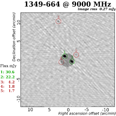
Figure 5: Example of a 9 GHz image of around 2FGL source J1353.5$-$6640. Flux densities were not corrected for beam attenuation. Objects 3–8 were flagged out. The gray area in the center of the image shows the error ellipse with the probability 99 per cent to find there J1353.5$-$6640.

At this point we visually checked every cleaned image. We have developed a web-application that allows us to interactively examine each image and flag those point sources found with imsad that appear to be spurious or lie far away from the pointing direction. For 7 per cent of the images we manually adjusted parameters for inversion and cleaning, such as image size, pixel size, offset of image center, and the number of CLEAN iterations. Figure 5 provides an example of one of the ATCA images. Sources 4–8 have a signal-to-noise ratio (SNR) in the range 5.5–6.7 — not sufficient for a reliable detection in the absence of other information. There are two sources within the 99 per cent localisation error ellipse of J1353.5$-$6640. Source 1 has a spectral index of $-$0.33, while source 2 has a spectral index of $-$1.00. Source 1 was also detected in the ATPMN survey (McConnell et al., 2012) as J135340.1$-$663957 with flux densities $43\pm 6$ and $28\pm 10$ mJy at 4.8 and 8.6 GHz respectively. There is also a strong X-ray source 1RXS J135341.1$-$664002 within 7 arcsec of source 1. Tsarevsky et al. (2005) observed its optical counterpart with the VLT,, which is within 1.7 arcsec of source 1, and reported a featureless spectrum. This suggests its classification as a BL Lac type. This additional information presents a strong argument in favour of association of source 1 with 2FGL J1353.5$-$6640.

Source 3 was flagged out because it lies 10.3 arcmin from the pointing direction. The beam power at 9 GHz drops by a factor of 2 at 2.7 arcmin and has the first minimum at 6.5 arcmin. In fact, source 3 lies within 1 arcsec, i.e. within its position error, from J1353-6630 detected in the Australia Telescope 20 GHz Survey (AT20G) carried out with ATCA at 20 GHz (Murphy et al., 2010). The AT20G catalogue reports a flux density of 322 mJy at 8 GHz. The flux density measured from our observations is 77 times weaker because it was detected by a sidelobe of the beam. We did not try to calibrate source flux densities for objects that had offsets from the pointing direction beyond where the beam power falls below 0.2; 400 arcsec at 5 GHz and 250 arcsec at 9 GHz. For sources that lay within these limits we corrected their flux densities for beam attenuation $P(\theta)$ using an approximation of the beam pattern measured by Wieringa & Kesteven (1992) in the form of

$$P(\theta)=\frac{\displaystyle 1}{\displaystyle\displaystyle\sum_{k=0}^{k=4}C_{k}(\theta\,f)^{2k}}$$ (15)

where $\theta$ is the distance from the pointing direction, $f$ is the observing frequency, and $C_{k}$ are coefficients that approximate beam pattern measurements.

4 Results

Table 1: The first 8 rows of 146 objects detected at both 5 and 9.0 GHz. The table columns are explained in the text. The full table is available in the electronic attachment.

2FGL name	IAU name	Fl	$\alpha$	$\delta$	$\Delta\alpha$	$\Delta\delta$	$F_{5}$	$F_{9}$	$\sigma_{5}$	$\sigma_{9}$	Sp5	Sp9	$\sigma$Sp5	$\sigma$Sp9	Sp	$\sigma$Sp	D	N$\sigma$	$F_{1}$	$C_{1}$	1GHz ID	WISE ID
			hr  min  sec	${}^{\circ}\hskip 5.0pt{}^{\prime}\hskip 5.0pt{}^{\prime\prime}$	′′	′′	mJy	mJy	mJy	mJy							′	′	mJy
(1)	(2)	(3)	(4)	(5)	(6)	(7)	(8)	(9)	(10)	(11)	(12)	(13)	(14)	(15)	(16)	(17)	(18)	(19)	(20)	(21)	(22)	(23)
J0031.0$+$0724	J0031+0724	f	00 31 19.69	$+$07 24 53.8	0.8	1.0	9.6	7.5	0.4	1.0	$-$0.21	$-$9.90	0.24	$-$9.90	$-$0.49	0.29	3.4	1.5	11.6	N	003119$+$072456	J003119.70$+$072453.6
J0102.2$+$0943	J0102+0944	a f	01 02 17.12	$+$09 44 10.4	0.6	0.8	14.7	16.4	0.3	0.4	0.40	$-$0.11	0.12	0.26	0.22	0.07	1.2	0.4	11.0	N	010217$+$094407
J0116.6$-$6153	J0116-6153	a f	01 16 19.70	$-$61 53 43.0	0.5	0.8	33.5	30.5	0.3	0.6	$-$0.04	$-$0.30	0.05	0.20	$-$0.19	0.05	2.7	1.4	24.0	S	011619$-$615343	J011619.59$-$615343.5
J0116.6$-$6153	J0116-6156	f	01 16 43.97	$-$61 56 53.3	0.6	0.8	17.5	15.8	0.4	1.3	$-$0.31	$-$9.90	0.14	$-$9.90	$-$0.20	0.18	3.7	1.7	33.0	S	011643$-$615653
J0116.6$-$6153	J0116-6150		01 16 56.83	$-$61 50 12.5	0.9	1.1	7.1	5.4	0.4	1.2	$-$1.04	$-$9.90	0.29	$-$9.90	$-$0.54	0.47	3.5	1.6	43.0	S	011656$-$615013
J0143.6$-$5844	J0143-5845	a f	01 43 47.45	$-$58 45 51.8	0.5	0.8	24.0	22.3	0.2	0.4	$-$0.18	$-$0.47	0.06	0.17	$-$0.15	0.04	1.5	1.2	26.0	S	014347$-$584550	J014347.39$-$584551.3
J0316.1$-$6434	J0316-6437	f	03 16 14.11	$-$64 37 30.8	0.6	0.9	15.7	12.5	0.4	1.0	0.18	$-$9.90	0.15	$-$9.90	$-$0.46	0.16	3.5	1.5	12.0	S	031614$-$643732	J031614.31$-$643731.4
J0409.8$-$0357	J0409-0400	a f	04 09 46.58	$-$04 00 02.4	0.5	0.8	89.9	87.7	0.3	0.7	0.35	$-$0.56	0.02	0.08	$-$0.05	0.02	2.4	1.1	39.1	N	040946$-$040003	J040946.57$-$040003.4

In summary, we detected 571 objects in 338 fields. Of these, 146 objects have position offsets beyond the areas of 99 per cent probability of the 2FGL positions. These objects were discarded from further analysis.

The rms of the images is typically in the range of 0.15–0.25 mJy. The FWHM size of the restored beam is typically 35 arcsec at 5 GHz and 20 arcsec at 9 GHz. The detection limit is 1.8 mJy for sources in the center of the field of view and 9 mJy at the edge of the field of view, at 6.5 arcmin. There are 23 fields that have a number of resolved objects, for instance the field around 2FGL source J1619.7$-$5040 which corresponds to the HII region G332.8$-$0.6 (Kuchar & Clark, 1997). Although the data analysis pipeline selected sources that it considers as “points”, these are actually hot spots in an extended Galactic object rather than separate compact extragalactic sources. Imaging of an extended object using 2–4 scans with a five-element array gives inconclusive results. We flagged sources from such fields as possibly extended. Extra care must be taken when dealing with these objects.

We cross-matched all remaining sources against the NVSS (Condon et al., 1998), SUMSS version 2.1 of 2012 February 16 (Bock, Large & Sadler, 1999; Mauch et al., 2003), MGPS-2 (Murphy et al., 2007), and WISE (Wright et al., 2010) catalogues. The NVSS catalogue is derived from VLA observations at 1.4 GHz and the SUMSS and MGPS-2 catalogues are derived from observations at 0.843 GHz with the Molonglo Observatory Synthesis Telescope. These catalogues have similar resolutions of $\sim\!40$ arcsec and are complimentary to each other as they cover different areas of the sky. We used a search radius of 20 arcsec to find counterparts in the NVSS, SUMSS and MGPS-2 catalogues, and $2\sigma$ position uncertainties of the ATCA coordinates for matching to a WISE object.

We have 160 matches in the WISE catalogue, 193 matches in NVSS, 59 matches in SUMSS, and 54 matches in MGPS-2. Since the average positional error of WISE is rather small, 0.25 arcsec, the mathematical expectation of the number of background WISE sources that fall within the $2\sigma$ error ellipse of ATCA position (in the case that the ATCA detections and WISE objects are physically unrelated) is only 10. We found matches for 16 times more sources, roughly 1/3 of our list. Thus, we conclude that the majority of the ATCA–WISE matches are real.

The NVSS catalogue contains objects with declinations $>-40\degr$. We have 243 ATCA detections with $\delta>-40\degr$ and 191 of these, i.e. 77 per cent, have a counterpart in NVSS. Among the 181 ATCA detected objects with declinations $<-40\degr$, 63 per cent have counterparts in SUMSS and MGPS-2. We have less counterparts with declinations below $-40\degr$ because these catalogues are not as deep as NVSS: their limiting peak brightness is 6 mJy beam^-1 at $\delta\leq-50\degr$ and 10 mJy beam^-1 at $\delta>-50\degr$, while NVSS has a limiting peak brightness 2.5 mJy.

We used these matches to re-calibrate position errors. We selected 92 matches that have flux densities brighter than 15 mJy at 1.4 GHz. NVSS positions of such sources are accurate to within less than 1 arcsec. We formed the dataset of position differences normalised to their standard deviations, which is the sum in quadrature of NVSS position uncertainties and position uncertainties from our ATCA observations. We used a reweighting model of the form $\sqrt{(r\,\sigma)^{2}+f^{2}}$ to bring the averaged normalised residuals close to one. We found the following scale-factors and error floors: 1.45 and 0.5 arcsec for right ascension and 1.80 and 0.75 arcsec for declination. We inflated our position errors according to this reweighting model.

For all detected sources we determined the spectral index within the subband. In addition, for sources detected at both subbands independently, we determined spectral indices between 5.5 and 9 GHz from their flux densities. In general, the spectral index between both subbands and from the low subband (5.5 GHz) spectra do not necessarily coincide because systematic errors affect the estimates in different ways and some sources may have spectra that deviate from the power law. In order to compare the consistency of spectral index estimates, we computed spectral indices using the low subband spectra for the sources that were detected in both bands as well. The scatter plot of this comparison is shown in Figure 6. We see that the spectral index across the [4.58, 6.42] GHz subband is slightly higher than the spectral index across [4.58, 9.91] GHz. This can be explained by a curvature in the spectrum. Results of this comparison demonstrate a reasonable consistency of spectral indices estimates using both approaches.

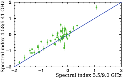
Figure 6: Comparison of source spectral indices from dual sub-band observations (horizontal axis) with the spectra determine from the low sub-band only (vertical axis).

In order to evaluate the significance of these $\gamma$-ray associations, we computed the likelihood ratios $\Lambda$. This is defined as the ratio of the probability that a radio counterpart will be found inside a disk of radius $d$ to the probability to find a background radio source with flux $S$ or greater outside the same disk:

$$\Lambda=\frac{\displaystyle e^{-n^{2}/2}}{\displaystyle N(1)\,S^{\,p}d^{2}/4}$$ (16)

where $n$ is the normalised arc $d$ between the radio and the 2FGL position, $N(1)andp$ are parameters of the $\log N(\log S)$ dependence that describes the number of sources $N$ with radio flux densities greater than $S$.

Among large radio surveys, the 4.85 GHz GB6 (Gregory et al., 1996) catalogue, with a FWHM of the beam of 3 arcmin, is the closest match to our ATCA observations at 5 GHz. We built a cumulative histogram log N–log S over 75,162 GB6 sources at 6.06 sr and fit a straight line to it in the interval of flux densities [30, 810] mJy. We obtain $N(1{\rm Jy})=965$ and $p=-1.3475$ from this analysis. We should note that these parameters are different than those we derived from the analysis of VLBI results because they are related to a different population of radio sources. The likelihood ratio describes our knowledge of how likely a radio source with a given flux density can be found at a given distance by chance. Sources with large $\Lambda$ are less likely located close to the $\gamma$-ray counterpart by chance.

The list of 424 sources falls into three categories:

Table 2: The first 8 rows of 229 objects detected in the 5 GHz subband only. The table columns are explained in the text. The full table is available in the electronic attachment.

2FGL name	IAU name	Fl	$\alpha$	$\delta$	$\sigma\alpha$	$\sigma\delta$	$F_{5}$	$\sigma_{5}$	Sp	$\sigma$Sp	D	N$\sigma$	$F_{1}$	$C_{1}$	1GHz ID	WISE ID
			hr  min  sec	${}^{\circ}\hskip 5.0pt{}^{\prime}\hskip 5.0pt{}^{\prime\prime}$	′′	′′	mJy	mJy			′	′	mJy
(1)	(2)	(3)	(4)	(5)	(6)	(7)	(8)	(9)	(10)	(11)	(12)	(13)	(14)	(15)	(16)	(17)
J0014.3$-$0509	J0014$-$0512		00 14 33.84	$-$05 12 48.0	3.3	3.8	2.7	0.6	$-$9.90	$-$9.90	5.1	1.5	4.3	N	001433$-$051244	J001433.86$-$051249.6
J0158.4$+$0107	J0158$+$0108		01 58 41.88	$+$01 08 23.7	3.2	4.5	3.0	0.7	$-$9.90	$-$9.90	4.2	1.1	17.6	N	015842$+$010817
J0200.4$-$4105	J0200$-$4109		02 00 20.91	$-$41 09 37.2	1.5	1.7	4.8	0.5	$-$9.90	$-$9.90	3.9	1.7				J020020.94$-$410935.6
J0226.1$+$0943	J0226$+$0937		02 26 13.81	$+$09 37 26.9	0.5	0.8	157.7	0.9	$-$0.22	0.03	5.8	2.5	374.6	N	022613$+$093726	J022613.70$+$093726.8
J0312.5$-$0914	J0312$-$0914		03 12 16.22	$-$09 14 17.5	3.1	2.4	11.3	1.5	$-$0.13	0.29	4.4	1.5	39.2	N	031216$-$091421	J031216.17$-$091418.7
J0312.5$-$0914	J0312$-$091A		03 12 18.26	$-$09 14 35.7	5.1	3.7	5.1	1.5	$-$9.90	$-$9.90	3.9	1.4				J031218.15$-$091436.4
J0312.5$-$0914	J0312$-$0919		03 12 21.67	$-$09 19 01.4	2.0	2.2	5.8	0.7	$-$9.90	$-$9.90	5.0	2.1	10.6	N	031221$-$091906	J031221.58$-$091902.8
J1046.8$-$6005	J1046$-$6005	ae	10 46 17.27	$-$60 05 21.6	0.5	0.8	264.2	1.8	$-$0.92	0.03	4.0	1.6

Table 3: The first 8 rows of 49 objects detected beyond 6.5 arcmin of the 5 GHz pointing centre, or detected only at 9 GHz. The table columns are explained in the text. The full table is available in the electronic attachment.

2FGL name	IAU name	Fl	$\alpha$	$\delta$	$\sigma\alpha$	$\sigma\delta$	D	N$\sigma$	$F_{1}$	$C_{1}$	1GHz ID	WISE ID
			hr  min  sec	${}^{\circ}\hskip 10.00002pt{}^{\prime}\hskip 10.00002pt{}^{\prime\prime}$	′′	′′	′	′	mJy
(1)	(2)	(3)	(4)	(5)	(6)	(7)	(8)	(9)	(10)	(11)	(12)	(13)
J0414.9$-$0855	J0415$-$0854		04 15 23.27	$-$08 54 26.5	3.6	3.5	6.9	2.1	10.3	N	041523$-$085425	J041523.13$-$085424.4
J0540.1$-$7554	J0539$-$7601		05 39 18.29	$-$76 01 30.6	13.7	4.4	8.0	2.2	79.0	S	053916$-$760131	J053916.48$-$760130.3
J0540.1$-$7554	J0540$-$7601		05 40 10.51	$-$76 01 54.0	11.8	3.9	7.7	2.2	37.0	S	054011$-$760156	J054011.59$-$760154.3
J0540.1$-$7554	J0541$-$7601		05 41 22.48	$-$76 01 09.6	18.9	5.8	8.1	2.4	31.0	S	054123$-$760108	J054123.16$-$760107.6
J0547.5$-$0141	J0547$-$0133		05 47 20.86	$-$01 33 30.9	1.4	1.8	8.1	1.4	22.1	N	054720$-$013327	J054720.85$-$013329.9
J0555.9$-$4348	J0555$-$4346		05 55 16.04	$-$43 46 30.7	1.8	1.4	7.1	2.2	144.0	S	055516$-$434631
J0555.9$-$4348	J0555$-$4345		05 55 19.57	$-$43 45 28.9	2.2	1.7	6.8	2.1	101.0	S	055519$-$434534
J0600.8$-$1949	J0600$-$1950	a	06 00 59.64	$-$19 50 39.4	1.0	1.0	2.0	0.5	96.7	N	060100$-$195049

1. Category I: 146 objects detected in both the 5 GHz and 9.0 GHz subbands within 2.7 arcmin of the pointing direction. We provide in Table 1 the $\gamma$-ray source name; IAU name of the detected radio source; tentative association status, estimates of its J2000 coordinates followed by $1\sigma$ uncertainties ($\sigma\alpha$ and $\sigma\delta$) in arcseconds (the uncertainties in Right Ascension are not scaled by $\cos\delta$); flux densities at 5 GHz and 9 GHz in mJy ($F_{5}$ and $F_{9}$) corrected for beam attenuation followed by their standard deviations ($\sigma_{5}$ and $\sigma_{9}$); spectral indices within the 5 and 9 GHz subbands Sp₅, Sp₉, and their standard deviations, followed by the spectral index from 5–9 GHz (Sp and $\sigma$Sp) computed from flux densities $F_{5}$ and $F_{9}$. Spectral index estimates with uncertainties greater than 0.4 are omitted. We provide the distance of a source from the pointing direction $D$, followed by $N\sigma$, the ratio of this distance to its standard deviation derived from the reported 2FGL position localisation errors. If the source was associated with an object either from NVSS, SUMSS, or MGPS-2 catalogues, its flux density at 1.4 GHz (NVSS) or 0.843 GHz (SUMSS and MGPS-2) is shown in column $F_{1}$ followed by the 1 GHz catalogue code ($N$ for NVSS, $S$ for SUMSS, $M$ for MGPS-2), and the source identifier in that catalogue. If the source was associated with a WISE object, its WISE source ID is shown in the last column.

   Column 3 shows two flags: “a” if the source has likelihood ratio greater than 10, and therefore, considered a likely association, “e” if the source is extended, and “f” if the source has a spectral index flatter than $-0.5$.

2. Category II: 229 objects detected only at 5 GHz within 6.5 arcmin of the pointing direction. We provide in Table 2 estimates of the flux density at 5 GHz corrected for beam attenuation. The contents of Table 2 is similar to Table 1, except columns $F_{9}$, $\sigma_{9}$, Sp, and $\sigma$Sp are excluded. The spectral index is computed only over the sub-band [4.58, 6.41] GHz. Spectral index estimates with uncertainties greater than 0.4 are omitted.

3. Category III: 49 objects either detected beyond 6.5 arcmin of the pointing direction or detected only at 9 GHz. Since calibration for beam attenuation becomes uncertain at large distances, we can only provide a lower limit estimate of their flux density: 20 mJy. Table 3 lists these sources. Its contents are similar to Table 2, except columns $F_{5}$ and $\sigma_{5}$, spectral index and its uncertainty are excluded.

   A fill value of $-9.9$ in all tables indicates a lack of information.

As can be seen from Figure 7, many of the unassociated Fermi sources are at low Galactic latitude. For the 30% of the sources in Tables 1–3 which lie within 1 degree of the Galactic plane, contamination of our ATCA images by Galactic HII regions, supernova remnants and planetary nebulae is common so careful work will be needed in the final identification process. As expected, flat-spectrum sources do not exhibit concentration to the Galactic plane.

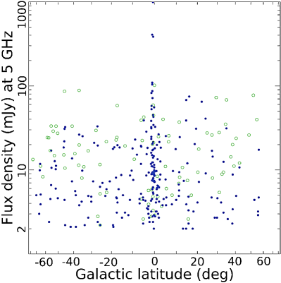
Figure 7: Dependence of the flux density of detected sources in categories I and II on galactic latitude. Flat spectrum sources are shown with green hollow circles. Other sources are shown with filled blue discs.

5 Concluding remarks

We found 424 counterparts within 99 per cent probability of localisation of 267 2FGL sources (Tables 1–3). For 141 2FGL sources more than one counterpart was found. Among 424 counterparts, 84 have a spectrum flatter than $-0.5$, 62 have a spectrum steeper than $-0.5$, and for 278 objects no spectral index has been determined. The flat spectrum sources are considered as tentatively associated with Fermi objects. For 128 sources the probability of association exceeds more than 10 times the probability to find a background source with that flux density by chance. These flags help to identify a subset of probable associations. However, taken alone, they do not establish a firm association. For instance, object J1045$-$5941 has a spectral index of 1.21, but it is a Galactic object ($\eta$ Carinae), not a blazar. Some compact HII regions and planetary nebulae may have flat spectrum. Additional information, e.g., from observations at other wavelengths, will help to identify a source associated with a $\gamma$-ray object.

Similarly, a steep spectrum does not rule out an extragalactic nature of an object. Kovalev (2009) presented several examples of steep-spectrum sources associated with Fermi objects. Detecting emission on parsec-scales will allow us to determine the nature of a radio source.

There are 46 objects from the fields that have a number of resolved objects. Many of these fields are associated with HII regions. Objects from these fields may in fact be hot spots of extended objects, not separate sources. Only 4 of them, i.e. 9 per cent, are associated with WISE objects, while 35 per cent of the remaining sources have counterparts from the WISE catalogue.

We did not find radio counterparts for 128 of our targets, roughly 1/3 of our list. Since for many sources the $3.035\sigma$ 2FGL position error ellipse exceeded the field of view of 6.5 arcmin at 5 GHz, we cannot claim there is no source brighter than 10 mJy in the field.

In the second phase of this project we plan to re-observe these fields in the mosaic mode to cover a larger area. This will allow us to detect all the sources in the 99 per cent probability of 2FGL localisation that are brighter than 2 mJy. We also plan to re-observe with ATCA those sources that were detected at 5 GHz, but are not detected at 9 GHz, and had position offsets exceeding the FWHM of the 9 GHz beam. To obtain more accurate positions and flux densities, we will also re-observe sources listed in Table 3, pointing to their positions found from this survey. New observations are scheduled in September 2013.

In the third phase of the project we will observe detected sources with the LBA to determine correlated flux densities from regions smaller than 50 mas. This will allow us to associate detected radio sources with blazars.

6 Acknowledgments

We wish to thank Mark Wieringa, Robin Wark, and Jamie Stevens for assistance in planning and carrying out the observations and processing the resulting data, and all the staff at the Paul Wild Observatory for their upkeep of the facility. We would like to thank James Condon and Greg Taylor for fruitful suggestions. F.K.S. acknowledges support by the NASA Fermi Guest Investigator program, grant NNX12A075G. The Australia Telescope Compact Array is part of the Australia Telescope National Facility which is funded by the Commonwealth of Australia for operation as a National Facility managed by CSIRO. This publication makes use of data products from the Wide-field Infrared Survey Explorer, which is a joint project of the University of California, and the JPL/California Institute of Technology, funded by the NASA.

7 Supporing information

Additional Supporting information may be found in the online version of this article:

Table S1. The 146 objects detected at both 5 and 9.0 GHz. The table columns are explained in the text.

Table S2. The 229 objects detected in the 5-GHz sub-band only. The table columns are explained in the text.

Table S3. The 49 objects detected beyond 6.5 arcmin from the 5- GHz pointing centre or detected only at 9 GHz. The table columns are explained in the text.

References

- Ackermann et al. (2012) Ackermann M., et al., 2012, ApJ, 753, 83
- Barr et al. (2013) Barr E. D., et al. 2013, MNRAS, 429, 1633
- Beasley et al. (2002) Beasley A. J., Gordon D., Peck A. B., Petrov L., MacMillan D. S., Fomalont E. B., Ma C. 2002, ApJS, 141, 13
- Bock, Large & Sadler (1999) Bock D. C.-J., Large M. I., Sadler E. M., 1999, AJ, 117, 1578
- Condon et al. (1998) Condon J. J., Cotton W. D., Greisen E. W., Yin Q. F., Perley R. A., Taylor G. B., Broderick J. J. 1998, AJ, 115, 1693
- Condon et al. (2011) Condon J., Darling J., Kovalev Y. Y., Petrov L. 2011, arXiv:1110.6252
- Fomalont et al. (2003) Fomalont E., Petrov L., McMillan D.S., Gordon D., Ma C., 2003, AJ, 126, 2562
- Gregory et al. (1996) Gregory P. C., Scott W. K., Douglas K., Condon J. J. 1996, ApJS, 103, 427
- Kellermann & Pauliny-Toth (1969) Kellermann, K. I., & Pauliny-Toth, I. I. K. 1969, ApJ, 155, L71
- Kovalev et al. (2007) Kovalev Y.Y., Petrov L., Fomalont E., Gordon D., 2007, AJ, 133, 1236
- Kovalev et al. (2009) Kovalev Y. Y., et al. 2009, ApJ, 696, L17
- Kovalev (2009) Kovalev Y. Y. 2009, ApJ, 707, L56
- Kuchar & Clark (1997) Kuchar T. A. & Clark F. O. 1997, ApJ, 488, 224
- Lister et al. (2009) Lister M. L., Homan D. C., Kadler M., Kellermann K. I., Kovalev Y.Y., Ros E., Savolainen T., Zensus J. A. 2009, ApJ, 696, L22
- Mauch et al. (2003) Mauch T., Murphy T., Buttery H. J., Curran J., Hunstead R. W., Piestrzynska B., Robertson J. G., Sadler E. M. (2003), MNRAS, 342, 1117
- McConnell et al. (2012) McConnell D., Sadler E. M., Murphy T., Ekers R. D. (2012), MNRAS, 422, 1527
- Murphy et al. (2007) Murphy T., Mauch T., Green A., Hunstead R. W., Piestrzynska B., Kels A. P., Sztajer P., 2007, MNRAS, 382, 382
- Murphy et al. (2010) Murphy T. et al. 2010, MNRAS, 420, 2403
- Nolan et al. (2012) Nolan P. L. et al., 2012, ApJS, 199, 31
- Petrov et al. (2005) Petrov L., Kovalev Y.Y., Fomalont E., Gordon D., 2005, AJ, 129, 1163
- Petrov et al. (2006) Petrov L., Kovalev Y.Y., Fomalont E., Gordon D., 2006, AJ, 131, 1872
- Petrov et al. (2008) Petrov L., Kovalev Y. Y., Fomalont E. B., Gordon D. 2008, AJ, 136, 580
- Petrov et al. (2009) Petrov P., Gordon D., Gipson J., MacMillan D., Ma C., Fomalont E., Walker R.C., Carabajal C., 2009, J Geod, vol. 83(9), 859
- Petrov & Taylor (2011) Petrov, L., Taylor, G. B., AJ, 2011, 142, 89
- Petrov et al. (2011a) Petrov L., Kovalev Y. Y., Fomalont E., Gordon D. 2011a, AJ, 142, 35
- Petrov et al. (2011b) Petrov L., Phillips C., Bertarini A., Murphy T., Sadler E. M., 2011b, MNRAS, 414(3), 2528
- Petrov (2012) Petrov L., 2012, MNRAS, 416, 1097
- Pushkarev & Kovalev (2012) Pushkarev A. B., Kovalev Y. Y., 2012, A&A, 544, 34
- Sault, Teuben & Wright (1995) Sault R. J., Teuben P. J., Wright M. C. H., 1995, In Astronomical Data Analysis Software and Systems IV, ed. by R. Shaw, H.E. Payne, and J.J.E. Hayes, ASP Conference Series, 77, 433
- Taylor et al. (2007) Taylor G. B., Healey S. E., Helmboldt J. F., et al. 2007, ApJ, 671, 1355
- Tsarevsky et al. (2005) Tsarevsky G. et al., 2005, A&A, 438, 949
-
Wieringa & Kesteven (1992)
Wieringa M. H., Kesteven M. J. 1992, ATNF Technical Memo, 39.2/010
http://www.atnf.csiro.au/observers/memos/d96b7e~1.pdf - Wilson et al. (2011) Wilson W. E. et al., 2011, MNRAS, 416, 832
- Wright et al. (2010) Wright E. L. et al., 2010, AJ, 140, 1868