Candidate Planets in the Habitable Zones of Kepler Stars

Abstract

A key goal of the Kepler mission is the discovery of Earth-size transiting planets in “habitable zones” where stellar irradiance maintains a temperate climate on an Earth-like planet. Robust estimates of planet radius and irradiance require accurate stellar parameters, but most Kepler systems are faint, making spectroscopy difficult and prioritization of targets desirable. The parameters of 2035 host stars were estimated by Bayesian analysis and the probabilities $p_{HZ}$ that 2738 candidate or confirmed planets orbit in the habitable zone were calculated. Dartmouth Stellar Evolution Program models were compared to photometry from the Kepler Input Catalog, priors for stellar mass, age, metallicity and distance, and planet transit duration. The analysis yielded probability density functions for calculating confidence intervals of planet radius and stellar irradiance, as well as $p_{HZ}$. Sixty-two planets have $p_{HZ}>0.5$ and a most probable stellar irradiance within habitable zone limits. Fourteen of these have radii less than twice the Earth; the objects most resembling Earth in terms of radius and irradiance are KOIs 2626.01 and 3010.01, which orbit late K/M-type dwarf stars. The fraction of Kepler dwarf stars with Earth-size planets in the habitable zone ($\eta_{\oplus}$) is 0.46, with a 95% confidence interval of 0.31-0.64. Parallaxes from the Gaia mission will reduce uncertainties by more than a factor of five and permit definitive assignments of transiting planets to the habitable zones of Kepler stars.

1 Introduction

The Kepler mission was launched in March 2009 with a mission to find Earth-size planets in the circumstellar “habitable zone” (HZ) of solar-type stars (Borucki et al., 2010). Broadly speaking, the HZ is considered the range of orbital semimajor axes over which the surface temperature on an Earth-like planet would permit liquid water. A narrower definition, adopted here, is that it is the range of stellar irradiance between the runaway “wet” greenhouse limit - beyond which a water-vapor saturated N₂-CO₂ atmosphere cannot radiate, and the CO₂ “snowball” limit below which this greenhouse gas condenses from an Earth-like atmosphere onto the poles (Kasting et al., 1993; Ishiwatari et al., 2007). This definition makes assumptions about planetary albedo, rotation rate (Spiegel et al., 2008), orbital eccentricity and obliquity (Williams & Pollard, 2003), extent of oceans (Abe et al., 2011), and thickness and composition of the atmosphere (Pierrehumbert & Gaidos, 2011). Many other factors besides stellar irradiation determine habitability (Gaidos et al., 2005). A planet in the canonical HZ may not be Earth-like, e.g., if it is geologically inactive (Kite et al., 2009), and there may be habitable environments outside the HZ, e.g. in the interiors of icy satellites (Reynolds et al., 1987). Nevertheless, an orbit in this HZ is a useful criterion for selecting objects for follow-up observations. Such prioritization is essential given that there are thousands of faint ($\sim$15th magnitude) Kepler systems that would require impractical amounts of telescope time to study.

Borucki et al. (2011) published a catalog of 54 (out of 1235) candidate planets or Kepler Objects of Interest (KOIs) with equilibrium emitting temperatures between 273 and 373 K, assuming an Earth-like albedo of 0.3. Kaltenegger & Sasselov (2011) noted the importance of albedo, specifically cloud cover, to equilibrium temperature, and computed inner and outer HZ boundaries based on the stellar irradiation criteria derived by Selsis et al. (2007) for high H₂O and high CO₂ atmospheres, respectively. They identified 76 possible habitable planets, depending on the assumed fractional cloud cover. They found that many of the Borucki et al. (2011) candidates were too hot for this habitability criterion and pointed out that errors in stellar parameters contribute most to the uncertainty of whether a planet orbits within the HZ.

Subsequently, a larger catalog (2300 KOIs, including some that are confirmed planets), was released (Batalha et al., 2013). Stellar parameters for KOI hosts, i.e. mass $M_{*}$ and radius $R_{*}$, were determined by fitting Yale-Yonsei model isochrones (Demarque et al., 2004) to values of effective temperature ($T_{*}$), surface gravity ($\log g$), and metallicity ([Fe/H]). Stellar parameters were derived from the photometry of the Kepler Input Catalog (KIC) and a model of stellar populations and Galactic structure (Brown et al., 2011). The Batalha et al. (2013) estimates of mass and radii assumed gaussian-distributed errors and employed standard deviations derived from a comparison between KIC-derived parameters and spectroscopic values. They revised the Brown et al. (2011) estimates of $\log g$ and $R_{*}$ for many stars. Batalha et al. (2013) assumed an albedo of 0.3 and efficient redistribution of heat over a planet’s surface, and identified 46 candidates with 185 K $<T_{eq}<$ 303 K.

However, the Brown et al. (2011) stellar parameters themselves are uncertain and in some aspects problematic. The vast majority of Kepler stars do not yet have measured parallaxes. KIC photometry must be corrected to place it in the Sloan system, and KIC-based effective temperatures are about 200 K hotter than estimates based on the infrared flux method (Pinsonneault et al., 2012). Moreover, uncertainties in stellar parameters, and hence incident irradiance, can be markedly non-gaussian. This is particularly true for solar-type stars for which photometry is unable to distinguish between main sequence and evolved (subgiant) stars (Brown et al., 2011; Gaidos & Mann, 2013). In such cases, standard deviations have limited utility in assessing statistical confidence.

A more rigorous approach is to estimate a probability that a planet orbits in the HZ, i.e. that the irradiance falls between the wet runaway greenhouse and CO₂ condensation limits. This can be done using the probability distribution function (PDF) of irradiance calculated from PDFs of the stellar parameters. The latter can be generated by comparing stellar models to observational constraints (i.e. photometry), calculating probabilities that the models can explain the data, and conditioning these by Bayesian priors. Each model and its associated value for irradiance is assigned a posterior probability, and the probability that the planet orbits in the HZ is the sum of the probabilities for those models having irradiances within the HZ limits, divided by the total probability for all models.

Bayesian estimation of stellar parameters has been applied to the KIC (Brown et al., 2011) as well as Hipparcos stars (Bailer-Jones, 2011). The analysis described here is distinguished by the use of corrected KIC photometry, synthetic isochrones and photometry from the Dartmouth Stellar Evolution database (Dotter et al., 2008) (see also Dressing & Charbonneau (2013), and new priors that describe distributions with mass (IMF), metallicity, age, and distance using recent models of the Galaxy (Vanhollebeke et al., 2009). In addition, it uses the duration and probability of planet transits to constrain stellar density (Plavchan et al., 2012).

I applied this procedure to the catalog of 2740 confirmed and candidate planets around 2036 Kepler stars released on 7 January 2013. I estimated the expected fraction of stars with planets orbiting in the HZ, and identified (candidate) planets with a better-than-even chance of having such orbits. I also cataloged Earth- to Super Earth-size planets with lower but non-zero probabilities. These objects are high-priority targets for follow-up observations to confirm the planets and better characterize their host stars.

2 Methods

2.1 Algorithm

I compared photometry for each star with sets of synthetic SDSS+2MASS grizJHK_s photometry from the isochrones of the Dartmouth Stellar Evolution Program (DSEP) (Dotter et al., 2008). With appropriate choices of mixing length and initial helium and heavy element fractions, DSEP is able to accurately reproduce the radius, luminosity, and convective boundary of the Sun, as well as the radii of fully convective stars in the hierarchical triple system KOI-126 (Feiden et al., 2011). DSEP uses PHOENIX model stellar atmospheres as boundary conditions; these LTE atmosphere models compare favorably to non-LTE calculations and observations for stars cooler than 7000 K (Hauschildt et al., 1999).

I compared up to six colors constructed with respect to the $r$ magnitude. According to Bayes’ theorem, the probability $P_{i}$ that the $i$th model (hypothesis) is supported by the photometry is equal to the probability that the colors ${c_{j}}$ can be produced by the model, multipled by a prior function $p_{i}$. Assuming gaussian-distributed errors in photometry, that probability is

$$P_{i}=p_{i}{\rm exp}\left[-\displaystyle\sum_{j}\frac{\left(c_{j}-k_{j}E^{i}_{B-V}-\hat{c_{j}}\right)^{2}}{2\sigma_{j}^{2}}\right],$$ (1)

where the summation is over up to six colors, ${\hat{c_{j}}}$ are the synthetic colors, ${\sigma_{j}}$ are the photometric errors, $k_{j}$ is the interstellar reddening coefficient for the color, and $E^{i}_{B-V}$ is the amount of reddening that is assigned to a particular model and star (see below). The normalization in Eqn. 1 is unimportant as it independent of the models and I identified the model which has the largest value of $P$. The prior is the product of individual priors for the mass, age, distance, and metallicity of the model, the intervening extinction, and, since at least one planet has been detected around each of these stars, a constraint on stellar density imposed by the duration of the transit (Plavchan et al., 2012).

Photometry and other data for the host stars of the KOIs were extracted from the KIC catalog available at the MAST database. KIC griz magnitudes were transformed to the Sloan system using the corrections determined by Pinsonneault et al. (2012). Standard errors for each bandpass were estimated using the expression $\sigma=\sigma_{0}10^{(m-m_{0})/2.5}$, where $\sigma_{0}=0.02,0.02,0.015,0.015,0.02,0.025,0.02$, and $m_{0}=15,15,15.3,15.3,13,11.75,10.8$, for grizJHK, respectively (Brown et al., 2011; Cutri et al., 2003). For griz the magnitude $m$ is the Kepler magnitude $K_{p}$ and for JHK_s it is the respective 2MASS magnitudes. Errors in color were calculated by assuming that errors in individual bandpasses are uncorrelated and adding the two corresponding such errors in quadrature.

Minimization of $P$ with respect to $E_{B-V}$ leads to a formula for the best-fit reddening for each model:

$$E_{B-V}=\frac{\displaystyle\sum_{j}k_{i}\left(c_{j}-\hat{c}_{j}\right)/\sigma_{j}^{2}}{\displaystyle\sum_{j}k_{j}^{2}/\sigma_{j}^{2}}$$ (2)

I adopted extinction coefficients $A$ of 3.758 ($g$), 2.565 ($r$), 1.874 ($i$), 1.377 ($z$), 0.272 ($J$), 0.173 ($H$), and ($K_{s}$), based on Girardi et al. (2005) and Chen et al. (2007).

I used the DSEP interpolator tool to construct a grid of isochrones with [Fe/H] $\in[-1.5,+0.5]$, at intervals of 0.1 dex, $\alpha/Fe$ $\in[-0.2,+0.4]$, at intervals of 0.2 dex, and ages $\in[1,12]$ Gyr at intervals of 0.5 Gyr. All models used a helium fraction $Y=0.245+1.5Z$, where $Z$ is the total heavy element abundance. I further restricted the selection to stars with initial masses between 0.1 and 2 solar masses, as late M and O, B, and early A-type stars are absent from the Kepler target list (Batalha et al., 2010). This restriction reduced the total number of models considered to 657,347.

Once the best-fit model with the maximum $P$ was found, additional models (typically a few dozen) with neighboring (difference less than 1.5 times the grid spacing) values of mass, age, [Fe/H], and [$\alpha$/Fe] were identified. A set of 100 linear interpolations between the best-fit model and each of these neighboring models was made and new probablities calculated using Eqn. 1. The interpolation yielding the highest value of $P$ was recorded.

2.2 Prior functions

Priors weight each DSEP model, i.e. each combination of initial mass, metallicity, age, and distance (modulus). The distance modulus for each star/model combination was computed in the $r$-band, i.e. $\mu_{r}=r-A_{r}E_{B-V}-\hat{M_{r}}$. A uniform prior is adopted for for the allowed range of [$\alpha$/Fe] between -0.2 and +0.4 dex. As a prior for initial stellar masses I adopt the tripartate initial mass function (IMF) of Kroupa (2002). Priors for age, metallicity, and distance modulus $\mu=m-M$ were constructed using the distributions of dwarf stars ($\log g>4$) with $K_{p}<16$ synthesized using TRILEGAL (Vanhollebeke et al., 2009). TRILEGAL accurately reproduces star counts over a wide range of magnitudes to very low galactic latitudes (Girardi et al., 2012). The simulated population was restricted to dwarfs to reflect the criteria of the selection of Kepler targets (Batalha et al., 2010). The (mostly default) values for key TRILEGAL parameters are the same as used in Gaidos & Mann (2013).

The resulting prior distributions (Fig. 1) have a median metallicity of -0.13, median age of 3.9 Gyr, and median $\mu=11.2$ ($\sim$1740 pc). The age distribution is complex because the population includes halo stars, which formed 11-12 Gyr ago, and disk stars, which started forming 9 Gyr ago in these simulations. TRILEGAL models the star formation rate in the disk in two steps, with the second occurring at about the epoch of the Sun’s formation. The paucity of stars younger than 1 Gyr is partly due to the fact that the Kepler field probes the stellar population that is $>100$ pc above the Galactic plane. Of course, stellar ages, metallicities, and distances are interrelated, but here they are used separately, providing broad constraints on the possible ranges of stellar parameters. The distance distribution is particularly important in allowing the finite scale height of the Galactic disk to prevent Malmquist bias from selecting arbitrarily distant and luminous stars.

The Kepler field is $\sim$10 degrees wide and close to the Galactic plane ($b\sim 13$ deg), so the stellar populations that are probed will vary significantly across the field. Using TRILEGAL, I synthesized the stellar population over a square degree centered at each of 84 Kepler half-CCD fields. Only those synthetic populations for CCD field centers with $b$ within 0.5 deg of a given Kepler star (about 10% of the total) were used to calculate priors for age, metallicity, and distance.

A prior for extinction $E_{B-V}$ necessarily involves information about the distribution of both stars and dust along each line of sight. However, by assuming that the spatial distributions of stars and dust are the same, the prior becomes particularly simple: a uniform distribution between 0 and total ($\infty$) extinction along the line of sight (see Appendix A). I found improved agreement with spectroscopy (Section 3.1) by conditioning $E_{B-V}$ with a uniform prior between 0 and $E_{B-V}(\infty)[1-exp(-z/h)]$, where $z$ is the vertical galactic distance above the Sun based on $\mu_{r}$, and $h$ is the dust scale height ($\sim$200 pc; Drimmel & Spergel, 2001). I adopted the Schlegel et al. (1998) Galactic reddening maps and interpolated the total extinction at the coordinates of each star using the IDL tools provided by the Princeton website. Models with optimal $E_{B-V}$ values outside this range are allowed, but reddening is limited to the maximum value and the models are penalized for the resulting disagrement between measured and model colors (Eqn. 1).

2.3 Constraints from the planet transit

The transit duration $\tau$ and orbital period $P_{K}$ of a transiting planet constrain stellar density (Plavchan et al., 2012) and can be used as an additional prior for stellar models. In the case of Kepler low-cadence data, the constraint is weakened by a lack of information about the orbit, specifically independent determination of the orbital eccentricity $e$ and the transit impact parameter $b$. The transit duration $D$ is:

$$D=\tau^{2/3}P_{K}^{1/3}\frac{\sqrt{(1-e^{2})(1-b^{2})}}{1+e\cos\phi},$$ (3)

where the stellar free-fall time is $\tau=2\sqrt{\hat{R_{*}}^{3}/(\pi G\hat{M_{*}})}$, $G$ is the gravitational constant, and $\phi$ is the argument of periastron relative to the line of sight to the star. Given $D$ and $P_{K}$ and a value for $\tau$ for each stellar model, $e$ can be written as a function of $b$ and $\phi$:

$$e(b,\phi,\Delta)=\frac{\sqrt{\left(1-b^{2}\right)\left(1-b^{2}-\Delta^{2}\sin^{2}\phi\right)}-\Delta^{2}\cos\phi}{1-b^{2}+\Delta^{2}\cos^{2}\phi},$$ (4)

where $\Delta\equiv D/(\tau^{2/3}P^{1/3})$. The eccentricity was calculated over a uniform grid of $b\in[0,1]$ and $\phi\in[0,2\pi]$. Each value of $e$ was assigned a probability, i.e. values not $\in[0,1]$ were assigned zero and others were assigned probabilities from a prior distribution of $e$. A Rayleigh distribution,

$$n(e)=\frac{e}{\sigma^{2}}e^{-e^{2}/(2\sigma^{2})},$$ (5)

was assumed, with $\langle e\rangle=\sigma\sqrt{\pi/2}$. Such a distribution has been used in a previous analysis of Kepler transit durations (Moorhead et al., 2011) and is motivated by dynamical theory (Jurić & Tremaine, 2008). Then the prior for the $i$th model from the duration of the transit is

$$p_{i}=\frac{1}{2\pi}\int_{0}^{1}db\int_{0}^{2\pi}d\phi\>n\left(e(b,\phi;\Delta_{i})\right).$$ (6)

To account for finite errors in transit duration, the prior can be calculated using multiple Monte Carlo-generated values of $D$ is repeated and then averaged. In the case of a multi-planet system $j=1...N$, the product of the individual transit duration priors $\prod_{j}p_{ij}(\Delta_{ij})$ was used. A value of $\sigma=0.2\sqrt{2/\pi}$ for the dispersion in eccentricities was used based on Moorhead et al. (2011). Figure 2 plots the prior for four values of $\langle e\rangle$.

2.4 Probability that a planet orbits in the habitable zone

Orbit-averaged irradiation is only weakly dependent on eccentricity for near-circular orbits. I assume near-circular orbits in which case the orbit-averaged irradiation in terrestrial units is approximately

$$I\approx\frac{\hat{L_{*}}}{L_{\odot}}\left(\frac{P_{K}}{365.24~{}{\rm d}}\right)^{4/3}\left(\frac{\hat{M_{*}}}{M_{\odot}}\right)^{2/3}.$$ (7)

A planet is defined to be in the HZ if $I_{out}<\bar{I}<I_{in}$, where the irradiance of the inner edge of the HZ for a 50% cloud-covered planet with efficient heat re-distribution is (Selsis et al., 2007)

$$I_{in}=\left[0.68-2.7619\times 10^{-5}\Theta-3.8095\times 10^{-9}\Theta^{2}\right]^{-2},$$ (8)

and the outer edge is:

$$I_{out}=\left[1.95-1.3786\times 10^{-4}\Theta-1.4286\times 10^{-9}\Theta^{2}\right]^{-2},$$ (9)

where $\Theta\equiv\hat{T_{*}}-5700$. These functions account for two major factors that introduce a dependence of the HZ boundaries on the stellar spectrum (and hence effective temperature): the dependence of Rayleigh scattering on wavelength, and the strong absorption by H₂O at redder wavelengths. Both act to lower the Bond albedo of an Earth-like planet around a cooler star relative to a hotter star (Kasting et al., 1993).

Kopparapu et al. (2013) re-calculated the irradiance boundaries using a cloud-free climate model based on new H₂O and CO₂ absorption coefficients. The revised boundaries are 10% lower (further out) than those of Selsis et al. (2007) but this difference is much smaller than that between the cloud-free and cloudy cases of Selsis et al. (2007). Because the Kepler survey is heavily biased towards shorter periods (Gaidos & Mann, 2013) and thus the high-irradiance (inner) edge of the HZ is more important to the determination of $p_{HZ}$, and because of the importance of clouds to this boundary, I elected to use the 50% cloud case of Selsis et al. (2007).

I determine whether a planet is in the HZ for each set of model stellar parameters $\hat{M_{*}}$,$\hat{L_{*}}$, and $\hat{T_{*}}$ with associated probability $P_{i}$. The probability $p_{HZ}$ that the planet is in the HZ is then:

$$p_{HZ}=\frac{\displaystyle\sum_{i\in HZ}P_{i}}{\displaystyle\sum_{i}P_{i}}$$ (10)

I consider candidate planets (or planets that may have satellites) as having greater-than-even odds of orbiting in the HZ ($p_{HZ}>0.5$) as well as having a most probable value of $\tilde{I}$ (with highest $P$) satisfying $I_{out}<\tilde{I}<I_{in}$.

3 Results

3.1 Comparison with spectroscopic parameters

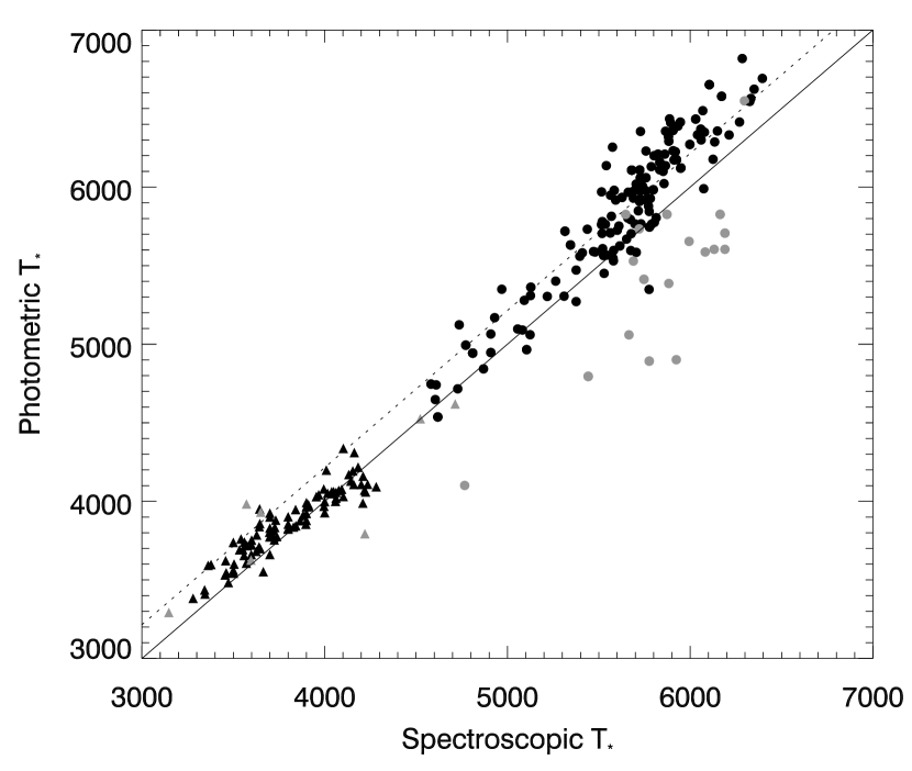
Figure 3: Comparison between effective temperatures based on photometry and spectroscopic values. Circles are solar-type stars from Buchhave et al. (2012) and Bruntt et al. (2012). Triangles are M dwarfs from Mann et al., in prep.. Black points are stars where all six photometric colors are available; grey points represent stars where at least one color is unavailable. The solid line is equality between the estimates and the dashed line represents the $\sim$215 K offset found by Pinsonneault et al. (2012).

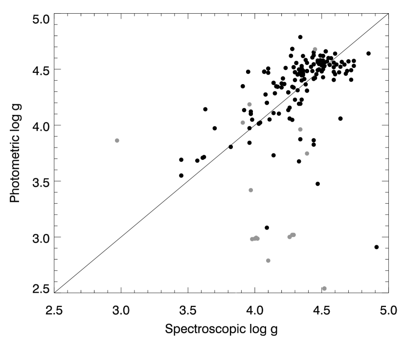
Figure 4: Comparison between photometric and spectroscopic estimates of surface gravities where the latter are taken from Buchhave et al. (2012) and Bruntt et al. (2012). Black points are stars where all six photometric colors are avialable; grey points represent stars where at least one color is unavailable. The solid line is equality between the two estimates.

Accurate estimates of stellar effective temperature $T_{*}$ and radius $R_{*}$ are crucial to assessing whether a planet is in the HZ, as together these largely determine the luminosity of the host star and the irradiance experienced by the planet on a given orbit. The inferred radius of a transiting planet also scales linearly with the estimated radius of the host star. The radii of distant Kepler stars cannot be directly measured, but spectroscopic values of $T_{*}$ and surface gravity $\log g$, the latter related to $R_{*}$, are available for some Kepler stars with planets (Bruntt et al., 2012; Buchhave et al., 2012, Mann et al., in prep.). Figures 3 and 4 compare photometry-based values of $T_{*}$ and $\log g$ with reported spectroscopic values. Photometric values for solar-type stars where all 6 colors are available average 208 K higher than spectroscopic values (Fig. 3). Pinsonneault et al. (2012) found that both the original KIC temperatures and spectroscopic estimates were $\sim$215 K cooler than determinations using the infrared flux method (IRFM). Thus the new photometric estimates are in line with IRFM values. The offset between photometric and spectroscopic temperatures is less (60 K) for M dwarfs; spectroscopic temperatures for these stars (Mann et al., in prep.) were determined by comparing spectra to synthetic spectra from PHOENIX/BT-SETTL models (Allard et al., 2011) and tuning the comparison using the temperature estimates of Boyajian et al. (2012).

Photometric $T_{*}$ for 16 stars is significantly lower than spectroscopic estimates. All but two of these are missing either $i$- or $z$-band photometry, or both. The importance of these bandpasses is not surprising as they are the only source of information in the wavelength range $0.7\mu{\rm m}<\lambda<1.1\mu{\rm m}$, just beyond the peak in emission from most of these stars, a spectral feature which most strongly constrains $T_{*}$. There are four stars with significantly ($>2\sigma$) hotter photometric estimates of $T_{*}$ relative to spectroscopy; only one of these is missing photometry. The reason(s) for the discrepancy among the other stars are unclear. One possibility is that the photometric source is a blend resolved by spectroscopy, or that the transit signal itself may be coming from a component of a blend which is dissimilar to the source of most of the light, and consequently the transit duration prior is skewing the stellar parameters. After removing the 208 K offset and ignoring stars with missing colors, the standard deviation between photometric and spectroscopic values of $T_{*}$ is $\sigma=180$ K for solar-type stars and 130 K for M dwarfs. This equals the performance of the analysis of Bailer-Jones (2011), but without the benefit of parallaxes.

Photometry-based estimates of $\log g$ are more discrepant with spectroscopic values, although an overall correlation is apparent (Fig. 4). About half of the most discrepant cases lack photometry in at least one bandpass, although many stars with missing photometry are assigned surface gravities close to the spectroscopic estimates. Although photometric colors involving the SDSS $u$ (Lenz et al., 1998) and $z$ (Vickers et al., 2012) bands can be used to discriminate between hotter main sequence and evolved stars, photometry is a much blunter tool to separate solar-type stars by luminosity class. While my analysis may only marginally improve this situation, it does quantify the uncertainties.

Among the KOI host stars with reported spectroscopic parameters are those with candidate HZ planets discussed below (Section 3.2). Buchhave et al. (2012) report spectroscopic parameters for three stars in Table 1, including Kepler-22b. The photometric values of $T_{*}$ are within 300 K of the corresponding spectroscopic estimates (Fig. 3). Muirhead et al. (2012) obtained $K$-band spectra for eight of these HZ stars and Mann et al. (in prep.) obtained visible-wavelength spectra for 18, including six of the Muirhead et al. (2012) targets (Table 1). Spectra confirm that all 20 are late K- or early M-type dwarfs. In general, the photometric temperatures of M dwarf KOI hosts agree with spectroscopic values except for the case of KIC 10027323 (hosting KOI 1596.02), where the photometric estimate (4636 K) is 800 K hotter than an IR spectroscopic value from Muirhead et al. (2012). The Muirhead et al. (2012) temperature are based on H₂O indices which saturate at temperatures hotter than $\sim$3800 K (Mann et al., in prep.)

3.2 Planets in the Habitable Zone

Of the 2740 confirmed and candidate planets, the analysis of 1 star (KIC 7746948 hosting KOIs 326.01 and 326.02) failed, as it is missing an $r$ magnitude and therefore cannot be analyzed by this procedure. The majority of (candidate) planets have essentially zero $p_{Hz}$ and 2604 (95%) have $p_{HZ}<0.01$.

Figure 5 shows the $p_{HZ}$ distribution of the 136 objects with $p_{HZ}>0.01$; the low-probability tail was excluded for clarity. The distribution is qusi-bimodal because some planets have posterior irradiance PDFs that are narrower than the irradiance difference across the HZ and hence are either very likely to be “in” ($p_{HZ}\approx 1$) or “out” ($p_{HZ}\approx 0$) of the HZ. The expected number of HZ planets in the catalog, the sum of $p_{HZ}$, is $\sim 73$. This figure does not change if $p_{HZ}<0.01$ are included, i.e. it is not determined by a very large number of low $p_{HZ}$ objects. Also plotted in Fig. 5 is the subset of planets which the maximum posterior probability (best-fit) models place outside the HZ. These cases arise when stellar parameters are poorly constrained; all but four have $p_{HZ}<0.5$, and I adopted this combination of criteria for identification of the highest-ranking HZ planets.

Two objects were excluded because they are unlikely to be planets: The radius of KOI 113.01 is between 1.3R_J and 0.37R_⊙ with 95% confidence and Batalha et al. (2013) list this KOI as having a “V-shaped” transit lightcurve indicative of an eclipsing binary. KOI 1226.01, has a minimum radius of 2R_J and a light curve suggestive of an eclipsing binary (Dawson et al., 2012). For seven candidates there is a $>10$% probabiity that the radius exceeds the theoretical upper limit for cool Jupiters (Fortney et al., 2010, $R_{p}\approx 1.2$R_J,). All of these cases could be explained by the very large errors in the radius of the host star, i.e. the inability of photometry to rule out an evolved star. Eight HZ candidates (KOIs 375.01, 422.01, 435.02, 490.02, 1096.01, 1206.01, and 1421.01) were excluded because their reported orbital periods are being based on the duration of a single transit and the assumption of a circular orbit, and have large uncertainties.

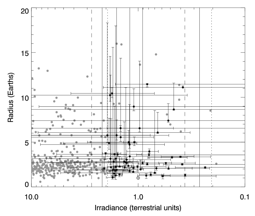
Figure 6: Radius and stellar irradiance of candidate and confirmed Kepler planets, and the Earth. Candidate planets in habitable zones are highlighted as black, all other KOIs are grey, and the vast majority of KOIs experience higher irradiances and fall outside the left-hand boundary of the plot. The error bars correspond to 95% confidence intervals. The solid, dotted, and dashed lines are the boundaries of the HZ for a 50% cloud-covered Earth like planet around a solar-type star (5780 K), an early M dwarf (3700 K) and late A-type (7800 K) star (Selsis et al., 2007).

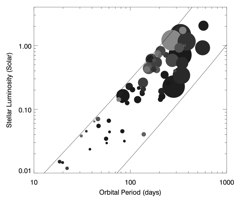
Figure 7: Luminosity of the host star vs. orbital period of candidate HZ planets ($p_{HZ}>0.5$) detected by Kepler, plus the Earth. The points are scaled to planet radius and the the darker the point, the more likely it is in the HZ. The two lines delimit the boundaries of the HZ for Earth-like planets with 50% cloud cover (Selsis et al., 2007). To plot the boundaries with these axes, it was necessary to assume simple but standard power-law relations between the luminosities, masses, and effective temperatures of main-sequence stars.

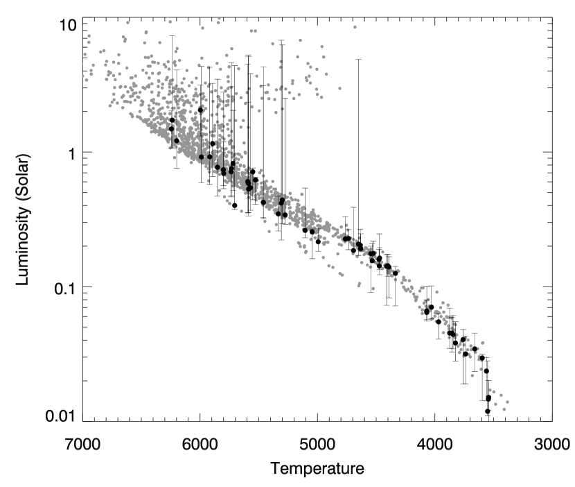
Figure 8: Hertzsprung-Russell diagram for host stars of 2739 candidate and confirmed Kepler planets. Black points are the 62 candidate HZ planets in Table 1. The error bars represent 95% confidence intervals on luminosity and are shown only for the candidate HZ planets.

The 62 remaining candidates with $p_{HZ}>0.5$ and most probable incident stellar irradiation in the HZ limits are listed in Table 1 and plotted in Figs. 6 and 7. The most probable and 95% confidence intervals for their irradiance and radius are given, and the stellar parameters of the model with highest posterior probability are reported. Figure 8 plots the host star parameters in a Hertzsprung-Russell diagram that includes all 2035 KOI host stars. Luminosities for a few host stars have very high upper bounds because the combination of photometry and priors cannot rule out the possibility that they are evolved with 95% confidence. All are most likely to be dwarfs except for KOI 1574.02, which I calculate has a probability of 53% of having $\log g<4.2$. Nearly all are assigned subsolar posterior metallicities but this is a result of the prior (Section 2.2) because photometry offers little constraint on metallicity.

Thirty-four planets were previously identified as possible HZ planets by Borucki et al. (2011), Kaltenegger & Sasselov (2011), Batalha et al. (2013), or Dressing & Charbonneau (2013). Most, but not all, of the others are candidates from the January 2013 release. The candidate around the brightest host star, KOI 87.01/Kepler-22b was previously flagged by Borucki et al. (2011) and Kaltenegger & Sasselov (2011) and confirmed by Borucki et al. (2012). The photometric estimate of effective temperature (5735 K) is consistent with two spectroscopic estimates (5518 and 5642 K), the inferred (maximum posterior probability) luminosity is slightly higher 0.9$L_{\odot}$ compared to 0.79$L_{\odot}$, and the inferred age of 8 Gyr is consistent with slow rotation and low flux in the core of the Ca II H and K lines (Borucki et al., 2012). The inferred stellar mass is identical (0.93$M_{\odot}$) to that determined by astroseismology. The preferred planet radius is 2.32R_⊕ and is within the errors of the previously published value of $2.38\pm 0.13$R_⊕, although the 95% confidence interval for this star is large.

KOI 250.04 is not (yet) a confirmed planet but is the outermost known member of the 4-planet Kepler-26 system containing two components (b and c) confirmed by transit timing variation (TTV) analysis (Steffen et al., 2012) and a fourth candidate (KOI 250.03) on the innermost orbit. The orbital period of KOI 250.04 ($P_{K}=46.83$ d) is suspicously close to one half of the period of a TTV signal seen near 90 d (Steffen et al., 2012). This analysis indicates that the host star of these planets has $T_{*}=4072$ K, i.e. is a late K dwarf. This is confirmed by two moderate-resolution visible-wavelength spectra which return 3996 K and 4067 K and a spectral type of K7.5 (Mann et al. in prep.), and an infrared spectrum which gives $T_{*}=3887$K (Muirhead et al., 2012). Steffen et al. (2012) report $T_{*}=4500$ K based on an SME analysis (Valenti & Piskunov, 1996) of a Keck-HIRES spectrum. However, SME effective temperatures are unreliable for very cool stars such as this. KOI 250.04 has a radius of about 2.4R_⊕, and it is of particular interest because further TTV analysis might constrain its mass.

The distribution with radius among these candidate HZ planets peaks in the super-Earth range ($\sim 2.5$R_⊕) and decreases with increasing radius, although there may be a cluster of candidates with radii approximately that of Jupiter. Presumably gas giants, these objects are potential hosts for habitable satellites (Kipping et al., 2009; Kaltenegger, 2010). For seven candidates there is a $>10$% probabiity that the radius exceeds the theoretical upper limit for cool Jupiters (Fortney et al., 2010, $R_{p}\approx 1.2$R_J,). In 5 of these cases, this can be explained by the very large errors in the radius of the host star (an evolved star cannot be ruled out).

Most of the smaller planets orbit the lowest-luminosity stars (Fig. 7), presumably because smaller planets are easier to detect around smaller stars. KOIs 2626.01 and 3010.01 are arguably the most “Earth-like” in terms of radius and irradiance. Table 1 also includes 10 additional candidate planets with $R_{p}<2$R_⊕ and $p_{HZ}>0.01$ (but $<0.5$). Five of these orbit late K or early M-type dwarfs, a figure that supports claims that these stars are the most promising locales to find Earth-size and Earth-like planets (Dressing & Charbonneau, 2013).

3.3 Not-so-habitable planets

Kaltenegger & Sasselov (2011) list 27 planets with semimajor axes between the inner edge (as defined by the onset of a runaway greenhouse) and outer edge of the HZ. Of these, 7 (KOIs 113.01, 465.01, 1008.01, 1026.01, 1134.02, 1168.01, 1232.01, were not retained in the Batalha et al. (2013) catalog. KOIs 113.01 and 1008.01 have V-shaped transit shapes and KOI 1232.01 has a large radius indicative of an elipsing binary. KOI 1134.02 exhibits “active pixel offset” meaning that the target star is not the source of the transit signal. KOI 1026.01 might be an artifact of systematics in the Kepler data (Batalha et al., 2013). KOIs 465.01 and 1168.01 were detected only with a single transit in the Borucki et al. (2011) catalog. Of the remaining 20, five (KOIs 139.01, 1099.01, 1423.01, 1439.01, and 1503.01) have $p_{HZ}<0.5$ and so do not appear in this catalog, although KOI-1423.01 is omitted marginally only so (0.47). KOI 1439.01 is most strongly ruled out ($p_{HZ}=0.06)$ because the revised $T_{*}$ is 274 K hotter and $R_{*}$ is 46% larger than the KIC values used by Kaltenegger & Sasselov (2011). The other 15 KOIs are retained in this catalog, along with 5 others from Kaltenegger & Sasselov (2011).

A comparison with the HZ candidates of Batalha et al. (2013) is problematic because they use an equilibrium temperature criterion which is dependent on the color/effective temperature of the host star. However, of the 24 candidate planets with 185K $<T_{eq}<$300K in Table 8 of Batalha et al. (2013), one KOI was later eliminated as a false positive (2841.01), and six KOIs (119.02, 438.02, 986.02, 1938.01, 2020.01, and 2290.01) have $p_{HZ}\ll 0.5$ and/or most probable $<I>$ outside the HZ limits. In each case, this is because the new estimates for $T_{*}$ are $\geq$200 K hotter than the previously published values, and because the most probably estimate of radius is significantly larger.

3.4 Fraction of Kepler stars with planets in the Habitable Zone

The calculations described above can be applied to the entire Kepler target catalog to estimate the fraction $f_{HZ}$ of stars with planets orbiting in the habitable zone. Obviously, the constraint on stellar density from the durations of transits could only be applied to KOIs. I estimated $f_{HZ}$ using the detection statistics of planets with $P<245$ d (at least 3 transits over 2 yr) around 122,442 stars with $\log g>4$ (KIC value) observed for at least 7 quarters of Q1-8.

This calculation identified the value of $f_{HZ}$ that maximizes the logarithmic likelihood (e.g., Mann et al., 2012)

$$\ln L=\displaystyle\sum_{i}^{D}\ln\left(f_{HZ}\langle d_{ik}\rangle\right)+\sum_{j}^{ND}\ln\left(1-f_{HZ}\langle d_{jk}\rangle\right),$$ (11)

where the first and second sums are over systems with and without detected planets with $R_{p}>2$R_⊕ and $P<245$ d in the HZ, respectively, $d_{ik}$ is the probability of detecting a planet in the HZ of the $i$th star described by the $k$th model, and $\langle\rangle$ represents the weighted average over all relevant models.

The detection completeness of the Kepler survey for planets wth $R_{p}<2$R_⊕ is still being established. I estimated $\eta$ for $R_{p}>0.8$R_⊕ by first computing the value for $R_{p}>2$R_⊕, then adjusting by the ratio 2.5 of $R_{P}>0.8$R_⊕ to $R_{p}>2$R_⊕ planets with $P<85$ d planets based on Table 3 of Fressin et al. (2013). This manuever assumes that the planet population inside 85 d is the same as that inside 245 d, but a distribution with radius would have to be assumed regardless because of severe incompleteness for small planets on wider orbits.

I calculated $d$ as the product of the geometric probability of transiting $d_{\rm transit}$, averaged over the HZ, and the fraction of planets $d_{signal}$ with $R_{P}>2$R_⊕ that would produce a transit large enough to be detected. For planets on circular orbits that are log-distributed with $P$ by a power-law with index $\beta$, the orbit-averaged geometric detection probability is:

$$d_{\rm transit}=0.00465\left(\frac{\hat{\rho}_{*}}{\rho_{\odot}}\right)^{-1/3}\left(\frac{P_{\rm in}}{\rm 1~{}yr}\right)^{-2/3}\frac{\beta}{\beta+\frac{2}{3}}\frac{1-\left(P_{\rm in}/P_{\rm out}\right)^{\beta+2/3}}{1-\left(P_{\rm in}/P_{\rm max}\right)^{\beta}},$$ (12)

where $P_{\rm in}$, $P_{\rm out}$, and $P_{\rm max}$ are the orbital periods at the inner and outer edges of the habitable zone and either the outer edge or the maximum period of the survey (245 d), respectively. These also depend on the luminosity and mass of the stellar model.

Based on a power-law distribution wth log radius (Howard et al., 2012), the fraction of planets $d_{\rm signal}$ generating a detectable transit was taken to be $(R_{\rm min}/2$R_⊕$)^{-1.92}$, if $R_{\rm min}>2$R_⊕, or unity otherwise. $R_{\rm min}$ is the minimum radius for detection (SNR = 7.1):

$$R_{\rm min}=0.29R_{\oplus}\frac{\hat{R}_{*}}{R_{\odot}}\left[{\rm CDPP}_{6}\sqrt{\frac{\rm 6~{}hr}{DN}}\right]^{1/2},$$ (13)

where CDPP₆ is the average 6 hr Combined Differential Photometric Precision over Q1-8 (in ppm), $D$ is the transit duration at the inner edge of the HZ, and $N$ is the number of transits in 2 yr for a planet with $P_{\rm in}$. Figure 9 shows a scatterplot and cumulative distributions of $P_{\rm in}$ and $R_{\rm min}$ for all stars assessed for these calculations. Forty-eight planets and $\sim$57,000 stars actually contributed to the statistics.

The presence of a planet in the HZ is known only with confidence $p_{HZ}$. To account for this, 10,000 Monte Carlo realizations of detections and non-detections were generated using the values of $p_{HZ}$ for each star, specifically new values of $p_{HZ}$ which represent the probability of a planet in the HZ having $R_{p}>2$R_⊕. The probability distributions with $f_{HZ}$ (Eqn. 11) were computed for each realization and summed. The summed distribution peaks at 0.332 with 95% confidence limits of 0.22 and 0.49. Based on the distribution in Fressin et al. (2013), the fraction of stars with a planet larger than 0.8R_⊕ in the HZ is $1-(1-0.332)^{2.5}=0.64$ (95% confidence interval of 0.46-0.81).

4 Discussion

Assumptions and systematic errors: There are several approximations and potential sources of systematic error that could affect the values of $p_{HZ}$ calculated here; I expect these values to evolve and that a few candidate planets may move in or out of the catalog as new data are incorporated, and the DSEP models are revised. However, the close correspondence between this catalog and previous ones suggests that the selection is relatively robust, although the relative rankings may change.

The constraint from the transit duration depends on orbital eccentricity, argument of periastron, and impact parameter. Uniform priors are appropriate choices for the last two parameters. However, a Rayleigh distribution for eccentricities (Eqn. 5) with mean $\langle e\rangle=0.2$, while consistent with Kepler data (Moorhead et al., 2011), is neither tightly constrained nor a unique choice (e.g. Shen & Turner, 2008). Indeed, a more refined prior would include the interrelationships with planet mass, orbital period, and the age of the system (Wang & Ford, 2011). I calculated the difference in $p_{HZ}$ resulting from changing $\langle e\rangle$ from 0.1 to 0.3. For the 62 candidates in the HZ, one half of the mean difference between the $p_{HZ}$ values is 0.019. This indicates that the transit duration constraint has a small but non-negligible effect on the identification of HZ planets.

These priors do not include the probability that a planet will transit its host star and be detected by Kepler, and thus be included in the KOI catalog. Such selection effects can be important in catalogs of transiting planets and their host stars (Gaidos & Mann, 2013). The geometric transit probability $R_{*}/a$, where $a$ is the semimajor axis, is proportional to $\tau^{2/3}$ and could be included readily enough: this factor will favor stellar models with larger radii. However, the probability of transit detection is primarily related to transit depth $\delta\approx(R_{p}/R_{*})^{2}$ and for a given $\delta$, a prior on stellar radius is ultimately a prior on planet radius. Some of these KOIs are nearly Earth-size, where the completeness of the Kepler survey is still being refined. Other KOIs are at or near theoretical limits of giant planet radii and any prior on stellar radii would have to include scenarios for astrophysical false positives. There are additional, but perhaps minor complexities: the probability of a transit occurring and being detected will also depend on $e$, $\phi$, $b$, as well as $D$, the transit duration. For these reasons, I do not include transit detection as a prior.

Equation 2 presumes a linear relationship between extinction in different bandpasses, i.e. that all can be linearly related to reddening $E_{B-V}$. This is not strictly correct, but is a fair approximation in the limit of small reddening. The median derived $E_{B-V}$ for these stars is only 0.08, corresponding to 0.25 magnitudes of extinction, and the 95 percentile value is 0.18. If the scale height of dust is smaller than that of stars, then the uniform prior derived under the assumption of identical gas and dust distributions (Appendix A) slightly underestimates the amount of reddening. Because reddening and temperatures derived from photometry are correlated, this assumption slightly underestimates the temperature and luminosities of stars as well.

The total number of candidate HZ planets is not sensitive to the precise irradiation limits. Because of detection bias towards short-period orbits, there are very few detected planets beyond the HZ (Fig. 6). For an Earth-like planet with 100% cloud cover, the runaway greenhouse irradiation limit is 23% higher than the 50% cloud-cover case (Selsis et al., 2007), but this admits only one additional candidate to the catalog. On the other hand, HZ calculations are sensitive to the precise value of $T_{*}$ because of the sensitivity of luminosity to effective temperature, and future refinements are worthwhile (see below). I do not account for systematic errors in the DSEP and TRILEGAL models themselves, but given the agreement with spectroscopy (Fig. 3) these are likely to be comparatively small. Of course, the HZ described here only applies to Earth-like planets with a surface pressure of $\sim 1$ bar. Planets with different surface gravities, pressures, and/or compositions may be habitable to larger distances (Pierrehumbert & Gaidos, 2011), or not at all (Gaidos, 2000).

The trouble with M dwarfs: The fundamental parameters of M dwarf stars have been a notorious challenge for models because of the difficulty in reproducing the observed mass-radius relation and their complex spectra. The DSEP models employed here accurately predict the radii of the two M dwarfs in the triply eclipsing hierarchical triple system KOI-126 (Feiden et al., 2011) (see also Feiden & Chaboyer, 2012). DSEP uses PHOENIX model atmospheres (Hauschildt et al., 1999) for both the stellar surface boundary conditions and to generate synthetic magnitudes. The spectroscopic temperatures presented here are calibrated using nearby interferometry targets (Boyajian et al., 2012) using the BT-SETTL flavor of PHOENIX models (Lépine et al., 2013), hence the good correlation between the two estimates is not surprising. Nevertheless, the offset of 60 K in $T_{*}$ is represents a $\sim$10% difference in $L_{*}$.

Another obstacle is that accurate modeling of the lightcurves of planets transiting M dwarfs must correctly account for significant limb darkening in the Kepler pass-band. Erroneous transit durations, acting through the prior described in Section 2.3, can bias the analysis towards models with incorrect radii: a 10% error in $R_{*}$ leads to a $\sim$30% error in $L_{*}$. This is sufficient to “move” a planet completely outside the HZ, or at least decrease the $p_{HZ}$ of a marginal HZ planet to $<$50%. Re-analyses of the Kepler transit lightcurves with improved limb-darkening models and re-derivation of the parameters of M dwarf KOI hosts are worthwhile, (e.g., Dressing & Charbonneau, 2013).

Future observations of Kepler stars: Stellar parameters based on analysis of photometry are no substitute for values based on high-resolution spectra, as long as the latter are carefully calibrated (see Pinsonneault et al., 2012). However, the median magnitude of the host stars of these planet is $K_{p}\approx 15.1$, and high-resolution spectroscopy is observationally expensive. The object most amenable to followup is, not coincidentally, Kepler-22b ($K_{p}=11.7$). The next brightest host star is that of KOI 1989.01 ($K_{p}=13.3$) and the rest are much fainter still and would require significant time on very large telescopes. However, this analysis generates a robustly-defined catalog to prioritize such work.

The Gaia (originally Global Astrometric Interferometer for Astrophysics) mission, scheduled for launch in October 2013, will obtain parallaxes with a sky-averaged, end-of-mission precision of 25 $\mu$as and 40 $\mu$as for 15th and 16th magnitude stars, respectively, and somewhat superior performance at the ecliptic latitude ($\sim$66 deg.) of the Kepler field (de Bruijne, 2012). To assess the potential of Gaia to refine the habitable zones of Kepler stars and the sizes of the planest that inhabit them, I re-calculated $P_{i}$ (Eqn. 1) for all models using a prior for distance modulus $p_{\mu}$ based on Gaia’s expected precision:

$$p_{\mu}={\rm exp}\>\left[-\frac{\left(\mu-\mu_{0}\right)^{2}}{2\sigma_{\mu}^{2}}\right],$$ (14)

where $\mu_{0}$ is the most probable distance modulus from the original analysis, and $\sigma_{\mu}\approx 8.7\times 10^{\mu_{0}/5-4}$ is the uncertainty in $\mu$ from a 40 $\mu$as precision in parallax.

The 95% confidence intervals in radius and stellar irradiance of the 62 HZ candidates were re-calculated and are shown in Fig. 10. The most probable values are unchanged, but the fractional errors in radius and irradiance are reduced by a factor of $\sim$5, from a median of 10% and 24%, respectively, to 1.7% and 5%, (equating 95% confidence intervals to $4\sigma$). The largest planets tend to orbit the hottest and most distant stars (Gaidos & Mann, 2013) and their parameters would retain the largest errors in this scenario. Typically, a few hundred DSEP models have appreciable $P$ values and contribute to the calculation for each star, but in a few cases the number is a few dozen and finite model grid size may determine the size of the errors. Values of $p_{HZ}$ for 50 of the 62 planets are $>0.97$. Spectroscopic values of $T_{*}$ accurate to 100 K would offer only modest further improvement (1.5% and 4.5% errors, respectively). Because these precisions reach or exceed levels of confidence in the predictions of the stellar models themselves as well as the absolute calibration of the photometry, refinement and verification of these may prove a more cost-efficient avenue for improvement. For example, Ugri and H_α photometry of much of the Kepler field has been obtained at the Isaac Newton Telescope (Greiss et al., 2012) and UBV photometry has been obtained at WIYN (Everett et al., 2012).

With such precision, it should be possible to locate planets within different regions of the HZ, e.g. near the inner edge, where low CO₂ atmospheres, and possibly high cloud fraction if there is a temperature-cloud feedback, should prevail: or the outer edge, where high CO₂ (von Paris et al., 2013) and possible water cloud-free atmospheres are more likely. Candidate HZ planets in multi-planet systems might be confirmed or even have masses determined by TTV. Although such advances may be difficult for planets around faint Kepler stars, this analysis offers a preview of the potential return from surveys of nearby, more observationally accessible stars, e.g. by the proposed TESS (Deming et al., 2009) and CHEOPS missions.

My calculations suggest that $\sim$64% of dwarf stars have planets orbiting in their habitable zones. The fraction of stars with Earth-size ($R_{p}=0.8-2$R_⊕) planets in the HZ ($\eta_{\oplus}$) is 0.46 (95% confidence limits of 0.31-0.64). This statistic will be greatly refined as the Kepler extended mission more thoroughly probes the HZ of solar-type stars, detection completeness is better quantified for smaller planets (Fig. 9), and the luminosities of the stars are better established (Fig 10). This estimate is only marginally higher than that of Traub (2012) ($\eta_{\oplus}$ = $0.34\pm 0.14$), who used the first 136 days of Kepler data. Also using Kepler data, Dressing & Charbonneau (2013) calculated that $0.15^{+0.13}_{-0.6}$ of M dwarfs have Earth-size (0.5-1.4R_⊕) planets in the HZ, but this was revised upwards to $0.48^{+0.12}_{-0.24}$ by Kopparapu (2013). Based on a radial velocity survey, Bonfils et al. (2011) estimated that 0.41${}^{+0.54}_{-0.13}$ of M dwarfs have planets with 1M_⊕$<M_{p}\sin i<$10M_⊕ in the HZ. The latter estimates are completely consistent with the value reported here for a wider range of spectral types, supporting optimism that numerous planets orbit in the habitable zones of stars all along the main sequence. Setting aside questions of formation and long-term orbital stability, these statistics also suggest favorable odds for finding a planet in the HZ of a component of the nearest star system, $\alpha$ Centauri.

Appendix A Derivation of a uniform probability distribution for extinction

If the probability distribution of stars with distance $x$ along the line of sight is $f(x)$ and the density of dust is $g(x)$, then the total column density of dust along the line of sight to a particular star is

$$A=A_{0}\int_{0}^{x}dx^{\prime}g(x^{\prime}),$$ (A1)

where $A_{0}$ is a constant factor. The probability of extinction to any randomly selected star falling between $A$ and $A+dA$ is

$$p(A)dA=f(x)\frac{dx}{dA}dA.$$ (A2)

However, from Eqn. A1, $dx/dA$ is simply $g(x)^{-1}$ and if $f(x)$ and $g(x)$ are identically distributed with $x$, then $p(A)$ is a constant, i.e. uniformly distributed over the range of allowed values.

Figure 1: Priors of age, metallicity, and distance modulus generated from 428,792 TRILEGAL-simulated stars with $K_{p}<16$ and $\log g>4$ in the Kepler field. The distributions of all synthetic stars is presented here, but only the $\sim$10% of stars with Galactic latitudes within 0.5 deg of a Kepler star of interest are used to generate actual priors.

Figure 2: Priors on the planet transit duration as a function of the parameter $\Delta\equiv D/(\tau^{2/3}P_{K}^{1/3})$, where $D$ is the transit duration, $\tau$ is the stellar free-fall time, and $P_{K}$ is the Keplerian orbital period, for circular orbits (solid line) and orbits with Rayleigh-distributed eccentricities with means of 0.1, 0.2, and 0.3.

Figure 5: Distribution of $p_{HZ}$, the probability that a Kepler confirmed or candidate planet orbits in its host star’s habitable zone. For clarity, only the 136 planets with $p_{HZ}>0.01$ are shown. The filled histogram is the $p_{HZ}$ distribution of the subset of objects with maximum posterior probability (best-fit) irradiances outside the habitable zone.

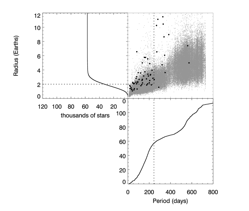
Figure 9: Upper right: scatter plot of minimum detectable planet radius $R_{\rm min}$ vs. orbital period at the inner edge of the habitable zone $P_{\rm in}$ for 122,442 Kepler stars observed for at least seven of Quarters 1-8 (grey points). Black points are the candidate HZ planets listed in Table 1. Bottom right: cumulative distribution with $P_{\rm in}$. Upper left: cumulative distribution with $R_{\rm min}$ for stars with $P_{\rm in}<245$ d. Dashed lines indicate the boundaries used to calculate the fraction of stars with planets in the habitable zone.

Figure 10: Reduction in the uncertainties in planet radius and stellar irradiation expected from inclusion of Gaia parallax measurements with 40 $\mu$as errors. Compare to Fig. 6.

Table 1: Candidate Planets in the Habitable Zones of Kepler Stars

		Planet Parameters								Stellar Parameters
KOI	KIC	$p_{HZ}$	Period	Irradiance ($I_{\oplus}$)			Radius (R⊕)			$T_{*}$	log $g$	[Fe/H]	$L_{*}$	$M_{*}$	Age	Commentb
			(days)	MPa	LLa	ULa	MPa	LLa	ULa	(K)			($L_{\odot}$)	($M_{\odot}$)	(Gyr)
87.01	10593626	0.64	289.9	1.29	0.99	7.23	2.32	2.00	5.91	5735	4.43	-0.2	0.90	0.93	7.8	Bo11,KS11,Bu12,Kepler-22b
250.04	9757613	1.00	46.8	1.33	0.99	1.53	2.16	1.91	2.22	3969	4.75	-0.3	0.05	0.51	8.6	Ma13,DC13,Kepler-26
351.01	11442793	0.93	331.6	1.76	1.27	2.39	10.44	9.38	12.95	6244	4.37	-0.4	1.48	0.94	5.7	Bo11,KS11
401.02	3217264	0.95	160.0	2.02	1.33	2.11	3.74	3.18	3.59	5528	4.52	-0.2	0.62	0.89	5.5	Bo11,KS11
433.02	10937029	0.99	328.2	0.82	0.51	0.88	11.46	9.20	10.65	5551	4.52	0.1	0.71	1.00	1.5	Bo11,KS11
463.01	8845205	0.93	18.5	1.64	1.05	2.18	1.82	1.34	2.17	3542	4.95	-0.5	0.02	0.34	1.2	Mu12,Ma13,DC13
465.01	8891318	0.55	349.9	1.67	1.03	7.05	3.63	2.89	7.77	6237	4.40	-0.2	1.73	1.15	1.4	KS11
518.03	8017703	1.00	247.4	0.55	0.35	0.58	2.66	2.40	2.75	5045	4.64	-0.5	0.26	0.69	6.4
622.01	12417486	0.74	155.0	1.59	1.06	22.63	5.76	4.94	26.68	5300	4.55	-0.3	0.44	0.81	7.5	Bo11,KS11
682.01	7619236	0.94	562.1	0.52	0.33	2.42	7.40	6.16	17.47	5918	4.51	-0.3	0.92	0.99	1.4	KS11,Bu12
701.03	9002278	1.00	122.4	1.20	1.02	1.50	1.79	1.78	1.98	4994	4.68	-0.5	0.22	0.68	1.7	Bo11,KS11,Bu12
812.03	4139816	0.73	46.2	1.62	1.33	2.33	2.23	2.01	2.32	4029	4.72	-0.4	0.07	0.57	1.5	Bo11,KS11,Mu12,Ma13
854.01	6435936	1.00	56.1	0.68	0.46	0.88	2.08	1.71	2.34	3661	4.80	0.0	0.03	0.49	2.1	Bo11,KS11,Mu12,Ma13,DC13
881.02	7373451	0.99	226.9	0.79	0.59	1.07	3.96	3.82	4.45	5334	4.64	-0.4	0.35	0.76	2.0	KS11
902.01	8018547	1.00	83.9	1.46	1.10	1.75	6.55	5.56	7.04	4471	4.63	-0.1	0.16	0.71	5.8	Bo11,KS11,Mu12
1209.01	3534076	0.80	272.1	0.97	0.56	8.47	6.54	4.95	22.53	5587	4.54	-0.4	0.59	0.84	5.5	Ba13
1268.01	8813698	0.51	268.9	1.83	1.15	6.16	10.24	8.75	20.25	6199	4.48	-0.2	1.21	0.99	2.1	KS11
1298.02	10604335	1.00	92.7	1.01	0.58	1.14	2.26	1.79	2.11	4337	4.67	-0.3	0.13	0.68	2.0	Ma13
1356.01	7363829	0.89	384.0	1.10	0.63	3.08	8.97	7.16	16.36	5893	4.40	-0.3	1.16	0.98	5.5
1361.01	6960913	1.00	59.9	1.11	0.93	1.34	2.12	1.91	2.30	4070	4.74	-0.3	0.07	0.54	1.9	Bo11,KS11,Mu12,Ma13
1375.01	6766634	0.75	321.2	1.20	0.78	5.66	4.73	4.09	11.76	5989	4.47	-0.5	0.92	0.86	6.0	Bo11,KS11
1422.02	11497958	0.98	19.9	1.50	1.24	1.58	1.39	1.29	1.39	3545	4.94	-0.3	0.01	0.33	8.5	Mu12,Ma13,DC13
1429.01	11030711	0.81	205.9	1.87	1.18	4.64	4.89	4.04	8.05	5719	4.47	-0.3	0.82	0.91	6.0	Bo11,KS11
1430.03	11176127	0.98	77.5	1.69	0.87	1.93	2.81	2.14	2.62	4546	4.64	-0.2	0.18	0.74	1.5	Ba13
1431.01	11075279	0.93	345.2	0.66	0.56	2.91	6.07	5.74	14.08	5587	4.57	-0.3	0.53	0.81	5.1	Ba13
1466.01	9512981	0.98	281.6	0.38	0.36	0.56	11.11	10.70	12.84	4763	4.63	-0.2	0.23	0.77	1.5	Ba13
1477.01	7811397	0.93	339.1	0.46	0.40	3.41	8.64	8.20	26.53	5275	4.61	-0.4	0.34	0.73	6.2	KS11
1527.01	7768451	0.62	192.7	1.82	1.14	11.15	3.15	2.61	8.56	5733	4.53	-0.2	0.75	0.96	2.0	Bo11,KS11
1574.02	10028792	0.99	574.0	1.09	0.70	1.67	4.99	3.77	5.28	5997	4.21	-0.2	2.05	1.05	6.7
1582.01	4918309	0.83	186.4	1.46	0.99	10.28	5.54	4.80	16.69	5571	4.58	-0.4	0.54	0.87	2.0	Bo11,KS11
1596.02	10027323	1.00	105.4	1.28	1.21	1.69	2.68	2.39	2.59	4636	4.63	0.2	0.20	0.76	1.5	Bo11,KS11,Mu12
1686.01	6149553	1.00	56.9	0.59	0.28	0.55	1.20	0.80	1.18	3597	4.83	-0.0	0.03	0.46	1.4	Ba13,Ma13,DC13
1739.01	7199906	0.79	220.7	1.59	0.97	7.16	1.90	1.56	4.43	5851	4.54	-0.4	0.77	0.93	2.0	Ba13
1871.01	9758089	1.00	92.7	1.24	1.20	1.65	2.34	2.26	2.68	4534	4.66	-0.3	0.16	0.70	1.5	Ba13
1876.01	11622600	1.00	82.5	1.28	0.76	1.53	3.04	2.25	3.26	4392	4.66	-0.2	0.14	0.71	1.9	Ba13
1879.01	8367644	0.84	22.1	1.11	1.03	2.64	1.69	1.58	2.81	3551	5.00	-0.2	0.01	0.30	2.0	Ma13,DC13
1902.01	5809954	0.69	137.9	0.24	0.11	0.28	2.18	1.42	2.39	3760	4.78	-0.3	0.04	0.50	1.2	Ba13,Ma13
1986.01	8257205	0.61	148.5	1.62	1.23	16.44	3.15	2.95	11.29	5460	4.62	-0.3	0.42	0.80	1.7
1989.01	10779233	0.65	201.1	1.80	1.38	7.21	2.19	2.04	4.93	5799	4.50	-0.5	0.69	0.79	8.5
2102.01	7008211	0.74	187.7	1.20	0.64	19.41	3.41	2.51	16.53	5307	4.56	-0.4	0.42	0.78	8.0	Ba13
2124.01	11462341	0.64	42.3	1.74	1.54	2.71	1.06	0.98	1.31	4069	4.75	-0.5	0.06	0.53	2.0	Ba13,Ma13
2410.01	8676038	0.58	186.7	2.08	1.59	3.36	2.05	1.89	2.74	5801	4.48	-0.4	0.74	0.81	8.5
2418.01	10027247	0.99	86.8	0.36	0.22	0.49	1.32	0.96	1.56	3739	4.84	-0.1	0.03	0.46	1.9	Ba13,Ma13,DC13
2469.01	6149910	0.95	131.2	0.95	0.95	1.99	1.95	2.01	2.71	4693	4.69	-0.3	0.19	0.67	1.2	Ba13
2474.01	8240617	0.76	176.8	1.73	1.05	15.42	1.88	1.52	6.57	5589	4.54	-0.4	0.59	0.84	5.5	Ba13
2626.01	11768142	1.00	38.1	0.84	0.51	1.06	1.26	0.92	1.43	3561	4.86	-0.0	0.02	0.43	1.1	Ba13,Ma13,DC13
2650.01	8890150	0.89	35.0	1.63	1.17	2.12	1.27	1.07	1.44	3855	4.78	-0.1	0.05	0.51	2.0	Ba13,Ma13,DC13
2681.01	6878240	0.84	135.5	1.23	1.08	2.53	4.99	4.82	6.75	5105	4.66	-0.4	0.26	0.72	2.0
2686.01	7826659	0.96	211.0	0.48	0.46	0.62	3.28	3.15	3.62	4631	4.64	-0.2	0.19	0.75	1.5
2689.01	10265602	0.77	165.3	1.95	1.14	14.51	5.75	4.32	17.97	5593	4.53	-0.4	0.60	0.84	6.1
2691.01	4552729	0.96	97.5	1.56	1.29	1.82	3.61	3.34	3.87	4736	4.63	-0.1	0.23	0.79	1.4
2703.01	5871985	1.00	213.3	0.40	0.37	0.48	3.35	3.16	3.56	4476	4.65	-0.2	0.16	0.73	1.5
2757.01	6432345	0.85	234.6	1.35	0.88	5.78	2.83	2.35	6.40	5735	4.54	-0.3	0.71	0.93	2.1
2762.01	8210018	0.99	133.0	0.82	0.72	1.01	2.54	2.35	2.72	4525	4.64	-0.1	0.18	0.75	2.1
2770.01	10917043	1.00	205.4	0.39	0.32	0.47	2.51	2.22	2.71	4401	4.66	-0.2	0.14	0.71	2.0	Ba13
2834.01	5609593	0.90	136.2	0.91	0.75	21.45	2.67	2.25	13.59	4651	4.63	-0.1	0.21	0.78	1.1
2882.01	5642620	0.55	75.9	1.49	1.40	2.58	2.28	2.11	2.73	4473	4.67	-0.3	0.14	0.68	1.4
2933.01	12416987	1.00	119.1	0.79	0.41	0.96	3.57	2.36	3.81	4411	4.66	-0.2	0.14	0.71	1.0
2992.01	8509442	1.00	82.7	0.52	0.40	0.79	2.07	1.76	2.48	3875	4.79	-0.2	0.05	0.50	1.5
3010.01	3642335	1.00	60.9	0.76	0.60	1.05	1.37	1.19	1.58	3845	4.79	-0.1	0.04	0.50	2.0
3034.01	2973386	0.66	31.0	1.68	1.23	2.42	1.49	1.21	1.77	3825	4.82	-0.2	0.04	0.48	1.5
3086.01	10749059	0.89	174.7	1.31	1.01	9.64	2.75	2.57	8.46	5462	4.62	-0.3	0.42	0.81	1.7
Other Planets with $R_{p}<2$R⊕ and $p_{HZ}>0.01$
172.02	8692861	0.38	242.5	2.44	1.63	4.81	1.88	1.64	2.44	6140	4.39	-0.2	1.38	0.97	5.1
775.03	11754553	0.15	36.4	2.12	1.84	2.55	1.81	1.67	1.96	4061	4.74	-0.3	0.06	0.54	1.9	Ma13
817.01	4725681	0.03	24.0	3.29	1.99	3.62	1.99	1.57	2.07	3900	4.73	-0.0	0.06	0.57	1.0	Bo11,Ma13,Mu12
1078.03	10166274	0.47	28.5	1.67	1.57	3.04	1.88	1.81	2.31	3790	4.84	-0.5	0.03	0.45	1.1	Ma13
2179.01	10670119	0.09	14.9	3.09	1.84	4.03	1.32	0.95	1.54	3606	4.87	-0.2	0.02	0.42	1.5	Ma13
2339.02	7033233	0.05	65.2	2.04	1.99	2.79	1.43	1.32	1.43	4551	4.66	-0.3	0.16	0.71	1.4
2373.01	10798331	0.16	147.3	2.16	1.89	7.89	1.96	1.86	3.84	5590	4.55	-0.2	0.56	0.82	5.9
2760.01	7877978	0.22	56.6	2.47	1.35	2.92	1.92	1.30	2.03	4510	4.65	-0.2	0.17	0.74	1.5
2862.01	6679295	0.14	24.6	2.84	1.71	3.45	1.72	1.32	1.85	3823	4.74	0.0	0.05	0.55	2.0
2931.01	8611257	0.39	99.2	2.47	1.65	24.73	1.95	1.61	7.29	5129	4.56	-0.2	0.38	0.80	7.5

References

- Abe et al. (2011) Abe, Y., Abe-Ouchi, A., Sleep, N. H., & Zahnle, K. J. 2011, Astrobiology, 11, 443
- Allard et al. (2011) Allard, F., Homeier, D., & Freytag, B. 2011, in Astronomical Society of the Pacific Conference Series, Vol. 448, 16th Cambridge Workshop on Cool Stars, Stellar Systems, and the Sun, ed. C. Johns-Krull, M. K. Browning, & A. A. West, 91
- Ammons et al. (2006) Ammons, S. M., Robinson, S. E., Strader, J., Laughlin, G., Fischer, D., & Wolf, A. 2006, ApJ, 638, 1004
- Bailer-Jones (2011) Bailer-Jones, C. A. L. 2011, MNRAS, 411, 435
- Batalha et al. (2010) Batalha, N. M., et al. 2010, ApJ, 713, L109
- Batalha et al. (2013) —. 2013, ApJS, 204, 24
- Belikov & Röser (2008) Belikov, A. N., & Röser, S. 2008, A&A, 489, 1107
- Bonfils et al. (2011) Bonfils, X., et al. 2011, ArXiv e-prints 1111.5019
- Borucki et al. (2010) Borucki, W. J., et al. 2010, Science, 327, 977
- Borucki et al. (2011) —. 2011, ApJ, 736, 19
- Borucki et al. (2012) —. 2012, ApJ, 745, 120
- Boyajian et al. (2012) Boyajian, T. S., et al. 2012, ApJ, 757, 112
- Brown et al. (2011) Brown, T. M., Latham, D. W., Everett, M. E., & Esquerdo, G. A. 2011, AJ, 142, 112
- Bruntt et al. (2012) Bruntt, H., et al. 2012, MNRAS, 423, 122
- Buchhave et al. (2012) Buchhave, L. a., et al. 2012, Nature, 486, 375
- Chen et al. (2007) Chen, P.-S., Yang, X.-H., & Zhang, P. 2007, AJ, 134, 214
- Cutri et al. (2003) Cutri, R. M., et al. 2003, 2MASS All Sky Catalog of point sources.
- Dawson et al. (2012) Dawson, R. I., Murray-Clay, R. A., & Johnson, J. A. 2012, ArXiv e-prints 1211.0554
- de Bruijne (2012) de Bruijne, J. H. J. 2012, Ap&SS, 341, 31
- Demarque et al. (2004) Demarque, P., Woo, J.-H., Kim, Y.-C., & Yi, S. K. 2004, ApJS, 155, 667
- Deming et al. (2009) Deming, D., et al. 2009, PASP, 121, 952
- Dotter et al. (2008) Dotter, A., Chaboyer, B., Jevremović, D., Kostov, V., Baron, E., & Ferguson, J. W. 2008, ApJS, 178, 89
- Dressing & Charbonneau (2013) Dressing, C. D., & Charbonneau, D. 2013, ArXiv e-prints 1302.1647
- Drimmel & Spergel (2001) Drimmel, R., & Spergel, D. N. 2001, ApJ, 556, 181
- Everett et al. (2012) Everett, M. E., Howell, S. B., & Kinemuchi, K. 2012, PASP, 124, 316
- Feiden & Chaboyer (2012) Feiden, G. A., & Chaboyer, B. 2012, ApJ, 757, 42
- Feiden et al. (2011) Feiden, G. A., Chaboyer, B., & Dotter, A. 2011, ApJ, 740, L25
- Fortney et al. (2010) Fortney, J. J., Baraffe, I., & Militzer, B. 2010, in Exoplanets (University of Arizon Press), 397
- Fressin et al. (2013) Fressin, F., et al. 2013, ApJ, 766, 81
- Gaidos et al. (2005) Gaidos, E., Deschenes, B., Dundon, L., Fagan, K., Menviel-Hessler, L., Moskovitz, N., & Workman, M. 2005, Astrobiology, 5, 100
- Gaidos & Mann (2013) Gaidos, E., & Mann, A. W. 2013, ApJ, 762, 41
- Gaidos (2000) Gaidos, E. J. 2000, Icarus, 145, 637
- Girardi et al. (2005) Girardi, L., Groenewegen, M. A. T., Hatziminaoglou, E., & da Costa, L. 2005, A&A, 436, 895
- Girardi et al. (2012) Girardi, L., et al. 2012, TRILEGAL, a TRIdimensional modeL of thE GALaxy: Status and Future, ed. A. Miglio, J. Montalbán, & A. Noels, 165
- Greiss et al. (2012) Greiss, S., et al. 2012, AJ, 144, 24
- Hauschildt et al. (1999) Hauschildt, P. H., Allard, F., & Baron, E. 1999, ApJ, 512, 377
- Howard et al. (2012) Howard, A. W., et al. 2012, ApJS, 201, 15
- Ishiwatari et al. (2007) Ishiwatari, M., Nakajima, K., Takehiro, S., & Hayashi, Y.-Y. 2007, Journal of Geophysical Research, 112, 1
- Jurić & Tremaine (2008) Jurić, M., & Tremaine, S. 2008, ApJ, 686, 603
- Kaltenegger (2010) Kaltenegger, L. 2010, ApJ, 712, L125