Abstract

Combining the Hardy-Littlewood $k$-tuple conjecture with a heuristic application of extreme-value statistics, we propose a family of estimator formulas for predicting maximal gaps between prime $k$-tuples. Extensive computations show that the estimator $a\log(x/a)-ba$ satisfactorily predicts the maximal gaps below $x$, in most cases within an error of $\pm 2a$, where $a=C_{k}\log^{k}x$ is the expected average gap between the same type of $k$-tuples. Heuristics suggest that maximal gaps between prime $k$-tuples near $x$ are asymptotically equal to $a\log(x/a)$, and thus have the order $O(\log^{k+1}x)$. The distribution of maximal gaps around the “trend” curve $a\log(x/a)$ is close to the Gumbel distribution. We explore two implications of this model of gaps: record gaps between primes and Legendre-type conjectures for prime $k$-tuples.

1 Introduction

Gaps between consecutive primes have been extensively studied. The prime number theorem [15, p. 10] suggests that “typical” prime gaps near $p$ have the size about $\log p$. On the other hand, maximal prime gaps grow no faster than $O(p^{0.525})$ [15, p. 13]. Cramér [4] conjectured that gaps between consecutive primes $p_{n}-p_{n-1}$ are at most about as large as $\log^{2}p$, that is, $\lim\sup(p_{n}-p_{n-1})/\log^{2}p_{n}=1$ when $p_{n}\to\infty$. Moreover, Shanks [28] stated that maximal prime gaps $G(p)$ satisfy the asymptotic equality $\sqrt{G(p)}\sim\log p$. All maximal gaps between primes are now known, up to low 19-digit primes (OEIS A005250) [29], [23]. This data apparently supports the Cramér and Shanks conjectures: thus far, if we divide by $\log^{2}p$ the maximal gap ending at $p$, the resulting ratio is always less than one — but tends to grow closer to one, albeit very slowly and irregularly.

Less is known about maximal gaps between prime constellations, or prime $k$-tuples. One can conjecture that average gaps between prime $k$-tuples near $p$ are $O(\log^{k}p)$ as $p\to\infty$, in agreement with the Hardy-Littlewood $k$-tuple conjecture [14]. Kelly and Pilling [17], Fischer [5] and Wolf [32] report heuristics and computations for gaps between twin primes ($k=2$). Kelly and Pilling [18] also provide physically-inspired heuristics for prime triplets ($k=3$); Fischer [6] conjectures formulas for maximal gaps between $k$-tuples for both $k=2$ and $k=3$. All of these conjectures and heuristics, as well as extensive computations, suggest that maximal gaps between prime $k$-tuples are at most about $\log p$ times the average gap, which implies that maximal gaps are $O(\log^{k+1}p)$ as $p\to\infty$.

In this article we use extreme value statistics to derive a general formula predicting the size of record gaps between $k$-tuples below $p$: maximal gaps are approximately $a\log(p/a)-ba$, with probable error $O(a)$. Here $a=C_{k}\log^{k}p$ is the expected average gap near $p$, and $C_{k}$ and $b$ are parameters depending on the type of $k$-tuple. This formula approximates maximal gaps better and in a wider range than a linear function of $\log^{k+1}p$. We will mainly focus on three types of prime $k$-tuples:

• $k=2$: twin primes (maximal gaps are OEIS A113274);

• $k=4$: prime quadruplets (maximal gaps are OEIS A113404);

• $k=6$: prime sextuplets (maximal gaps are OEIS A200503).

The observations can be readily applied to other $k$-tuples; however, numerical values of constants $C_{k}$ will change depending on the specific type of $k$-tuple. See, e. g., the following OEIS sequences for data on maximal gaps between prime $k$-tuples for other $k$:

• $k=3$: prime triplets (maximal gaps are A201596 and A201598);

• $k=5$: prime quintuplets (maximal gaps are A201073 and A201062);

• $k=7$: prime septuplets (maximal gaps are A201051 and A201251);

• $k=10$: prime decuplets (maximal gaps are A202281 and A202361).

2 Definitions, notations, examples

Twin primes are pairs of consecutive primes that have the form $\{p$, $p+2\}$. (This is the densest repeatable pattern of two primes.) Prime quadruplets are clusters of four consecutive primes of the form $\{p$, $p+2$, $p+6$, $p+8\}$ (densest repeatable pattern of four primes). Prime sextuplets are clusters of six consecutive primes of the form $\{p$, $p+4$, $p+6$, $p+10$, $p+12$, $p+16\}$ (densest repeatable pattern of six primes).

Prime $k$-tuples are clusters of $k$ consecutive primes that have a repeatable pattern. Thus, twin primes are a specific type of prime $k$-tuples, with $k=2$; prime quadruplets are another specific type of prime $k$-tuples, with $k=4$; and prime sextuplets are yet another type of prime $k$-tuples, with $k=6$. (The densest $k$-tuples possible for a given $k$ may also be called prime constellations or prime $k$-tuplets.)

Gaps between prime $k$-tuples are distances between the initial primes in two consecutive $k$-tuples of the same type. If the prime at the end of the gap is $p$, we denote the gap $g_{k}(p)$. For example, the gap between the quadruplets $\{11,13,17,19\}$ and $\{101,103,107,109\}$ is $g_{4}(101)=90$. The gap between the twin primes $\{17,19\}$ and $\{29,31\}$ is $g_{2}(29)=12$. Hereafter $p$ always denotes a prime. In the context of gaps between prime $k$-tuples, $p$ will refer to the first prime of the $k$-tuple at the end of the gap; we call $p$ the end-of-gap prime. (Note that primes preceding the gap might be orders of magnitude smaller than the gap size itself; e. g., the gap $g_{6}(16057)=15960$ starts at $\{97,101,103,107,109,113\}$; the gap $g_{6}(1091257)=1047480$ starts at $\{43777,43781,43783,43787,43789,43793\}$.)

A maximal gap is a gap that is strictly greater than all preceding gaps. In other words, a maximal gap is the first occurrence of a gap at least this size. As an example, consider gaps between prime quadruplets (4-tuples): the gap of 90 preceding the quadruplet $\{101,103,107,109\}$ is a maximal gap (i.e. the first occurrence of a gap of at least 90), while the gap of 90 preceding $\{191,193,197,199\}$ is not a maximal gap (not the first occurrence of a gap at least this size). A synonym for maximal gap is record gap. By $G_{k}(x)$ we will denote the largest gap between $k$-tuples below $x$. (Note: Statements like this will always refer to a specific type of $k$-tuples.) We readily see that

$$g_{k}(p) \leq G_{k}(p)\quad\mbox{ wherever $g_{k}(p)$ is defined, and}$$

$$g_{k}(p) = G_{k}(p)\quad\mbox{ if $g_{k}(p)$ is a maximal gap.}$$

In rare cases, the equality $g_{k}(p)=G_{k}(p)$ may also hold for non-maximal gaps $g_{k}(p)$; e. g., $g_{4}(191)=G_{4}(191)=90$ even though the gap $g_{4}(191)$ is not maximal.

The average gap between $k$-tuples near $x$ is denoted $\overline{g_{k}(x)}$ and defined here as

$$\overline{g_{k}(x)}=\frac{\displaystyle\sum_{{1\over 2}x\,\leq\,p-g_{k}(p)\,<\,p\,\leq\,{3\over 2}x}\mspace{-48.0mu}g_{k}(p)\hphantom{x}}{\mspace{-32.0mu}\displaystyle\sum_{{1\over 2}x\,\leq\,p-g_{k}(p)\,<\,p\,\leq\,{3\over 2}x}\mspace{-48.0mu}1}=\frac{\mbox{the sum of all gaps between $k$-tuples with }p\in[{1\over 2}x,{3\over 2}x]}{\mbox{total count of gaps between $k$-tuples with }p\in[{1\over 2}x,{3\over 2}x]}\,.$$

(The value of $\overline{g_{k}(x)}$ is undefined if there are less than two $k$-tuples with ${1\over 2}x\leq p\leq{3\over 2}x$.)

The expected average gap between $k$-tuples near $x$ (for any $x\geq 3$) is defined formally as $a=a(x)=C_{k}\log^{k}x$, where the positive coefficient $C_{k}$ is determined by the type of the $k$-tuples. (See the Conjectures section for further details on this.)

3 Motivation: is a simple linear fit for $G_{k}(p)$ adequate?

The first ten or so terms in sequences of record gaps (e. g., A113274, A113404, A200503) seem to indicate that maximal gaps between $k$-tuples below $p$ grow about as fast as a linear function of $\log^{k+1}p$. For twin primes ($k=2$), Rodriguez and Rivera [26] gave simple linear approximations of record gaps, while Fischer [6] and Wolf [32] proposed more sophisticated non-linear formulas. Why bother with any non-linearity at all? Let us look at the data. Table 1 presents the least-squares zero-intercept trendlines [16], [22] for record gaps between $k$-tuples below $10^{15}$ ($k=2$, 4, 6).

TABLE 1

Least-squares trendlines for maximal gaps between prime $k$-tuples ($k=2$, 4, 6).

	$1^{1}$Trendline equation for maximal gaps between prime $k$-tuples:
End-of-gap prime $p$	twin primes	prime quadruplets	prime sextuplets
	($k=2$; $\xi=\log^{3}p$)	($k=4$; $\xi=\log^{5}p$)	($k=6$; $\xi=\log^{7}p$)
$1^{1}$ $1<p<10^{6}$	$y=0.4576\xi$	$y=0.0627\xi$	$y=0.0016\xi$
$10^{6}<p<10^{9}$	$y=0.4756\xi$	$y=0.1031\xi$	$y=0.0147\xi$
$10^{9}<p<10^{12}$	$y=0.5203\xi$	$y=0.1245\xi$	$y=0.0181\xi$
$10^{12}<p<10^{15}$	$y=0.5628\xi$	$y=0.1451\xi$	$y=0.0249\xi$

Table 1 shows that, for a fixed $k$, record gaps between $k$-tuples farther from zero have a steeper trendline (when plotted against $\log^{k+1}p$). This is not a “one-slope-fits-all” situation! There is a good reason to expect that the same tendency holds in general for any $k$: As we will see in the next sections, there exist curves that predict the record gap sizes, on average, better than any linear function of $\log^{k+1}p$ — and the farther from zero, the steeper are these curves (approaching certain limit values of slope, $C_{k}$). Nevertheless, a linear approximation can also be useful; computations and heuristics suggest that a linear function of $\log^{k+1}p$ can serve as a convenient upper bound for gaps. For example: Maximal gaps between twin primes are less than $0.76\log^{3}p$. In what follows, we will combine the Hardy-Littlewood $k$-tuple conjecture with extreme value statistics to better predict the sizes of maximal gaps between prime $k$-tuples of any given type, accounting for their non-linear growth trend.

4 Conjectures

In this section we state several conjectures based on plausible heuristics and supported by extensive computations. As far as rigorous proofs are concerned, we do not even know whether there are infinitely many $k$-tuples of a given type — e. g., whether there are infinitely many twin primes for $k$ = 2. (The famous twin prime conjecture thus far remains unproven. A fortiori there is no known proof of the more general $k$-tuple conjecture described below.)

4.1 The Hardy-Littlewood $k$-tuple conjecture

The Hardy-Littlewood $k$-tuple conjecture [14], [25, pp. 60–68] predicts the approximate total counts of prime $k$-tuples (with a given admissible pattern):

$$\mbox{The total number of prime $k$-tuples below $x$}~{}\sim~{}H_{k}\int_{2}^{x}{dt\over\log^{k}t}.$$

The actual counts of $k$-tuples match this prediction with a surprising accuracy [25, p. 62]. The coefficients $H_{k}$ are called the Hardy-Littlewood constants. Note that, in general, the constants $H_{k}$ depend on $k$ and on the specific type of $k$-tuple (e. g., there are three types of prime octuplets, with two different constants). Hardy and Littlewood not only conjectured the above integral formula but also provided a recipe for computing the constants $H_{k}$ as products over subsets of primes. For example, in special cases with $k=2,4,6$ we have

$$H_{2} = 2\prod_{p\geq 3}{{p(p-2)}\over{(p-1)^{2}}}~{}\approx~{}1.32032\qquad\mbox{ (for twin primes),}$$

$$H_{4} = {27\over 2}\prod_{p\geq 5}{{p^{3}(p-4)}\over{(p-1)^{4}}}~{}\approx~{}4.15118\qquad\mbox{ (for prime quadruplets),}$$

$$H_{6} = {15^{5}\over 2^{13}}\prod_{p\geq 7}{{p^{5}(p-6)}\over{(p-1)^{6}}}~{}\approx~{}17.2986\qquad\mbox{ (for prime sextuplets)}.$$

These formulas for $H_{k}$ have slow convergence. Riesel [25] and Cohen [3] describe efficient methods for computing $H_{k}$ with a high precision. Forbes [8] provides the values of $H_{k}$ for dense $k$-tuples, or $k$-tuplets, up to $k=24$. The $k$-tuple conjecture implies that

• The sequence of maximal gaps between prime $k$-tuples of any given type is infinite. (Thus, all OEIS sequences mentioned in Introduction are infinite.)

• When $x\to\infty$, the largest gaps below $x$ will grow (asymptotically) at least as fast as average gaps, i. e., as fast as $O(\log^{k}x)$ or faster.

But exactly how much faster? Conjectures (D) and (E) below give plausible answers.

4.2 Conjectured asymptotics for gaps between $k$-tuples

Let $C_{k}$ denote the reciprocal to the corresponding Hardy-Littlewood constant: $C_{k}=H_{k}^{-1}$. The following formulas provide rough estimates of the gap $g_{k}(p)$ ending at a prime $p$:

(A) Average gaps between prime $k$-tuples near $p$ are $\overline{g_{k}(p)}\sim C_{k}\log^{k}p.$

(B) Maximal gaps between prime $k$-tuples are $O(\log^{k+1}p)$:

$$g_{k}(p)<M_{k}\log^{k+1}p,\quad\mbox{ where }M_{k}\approx C_{k}\quad\mbox{ (and possibly }M_{k}=C_{k}).$$

Defining the expected average gap near $x$ to be $a=C_{k}\log^{k}x$  ($x\geq 3$), we further conjecture:

(C) Maximal gaps below $x$ are asymptotically equal to $C_{k}\log^{k+1}x$:

$$G_{k}(x)\sim C_{k}\log^{k+1}x\quad\mbox{ as }x\to\infty,\quad\mbox{with probable error }O(a\log a).$$

(D) Maximal gaps below $x$ are more accurately described by this asymptotic equality:

$$G_{k}(x)~{}\sim~{}a\log(x/a)\quad\mbox{ as }x\to\infty,\qquad\mbox{ with probable error }O(a).$$

(E) For any given type of $k$-tuple, there exists a real $b$ (e. g., $b\approx{2\over k}$) such that the difference $G_{k}(x)-a(\log(x/a)-b)$ changes its sign infinitely often as $x\to\infty$.

A key ingredient in these conjectures is provided by the constants $C_{k}={H_{k}}^{-1}$:

$$C_{2}=H_{2}^{-1}\approx 0.75739,\qquad C_{4}=H_{4}^{-1}\approx 0.240895,\qquad C_{6}=H_{6}^{-1}\approx 0.057808.$$

Another key ingredient is a statistical formula: for certain kinds of random events occurring at mean intervals $a$, the record interval between events observed in time $T$ is likely near $a\log(T/a)$. In Appendix we derive this formula for $a=\mbox{const}$. Here, we heuristically apply this formula for a slowly changing $a$ (i. e., $a=C_{k}\log^{k}x$). For now, we can informally summarize the behavior of maximal gaps between $k$-tuples near $p$ as follows: Maximal gaps are at most about $\log p$ times the average gap.

4.3 Estimators for maximal gaps between $k$-tuples

Prime $k$-tuples are rare and seemingly “random”. Life offers many examples of unusually large intervals between rare random events, such as the longest runs of dice rolls without getting a twelve; maximal intervals between clicks of a Geiger counter measuring very low radioactivity, etc. Reasoning as in Appendix, one can statistically estimate the mathematical expectation of maximal intervals between rare random events by expressing them in terms of the average intervals:

$$\mbox{Expected maximal intervals}~{}=~{}a\log(T/a)+O(a),$$

where $a$ is the average interval between the rare events, and $T$ is the total observation time or length ($1\ll a\ll T$).

To account for the observed non-linear growth of record gaps between prime $k$-tuples (Table 1), we will simulate gap sizes using estimator formulas very similar to the above $(*)$. We define a family of estimators for the maximal gap that ends at $p$:

$$E_{1}(G_{k}(p)) = \max(a,\,a\log(p/a)-ba),\qquad\mbox{ probable error: $O(a);$ }$$ (1)

$$E_{2}(G_{k}(p)) = \max(a,\,a\log(p/a)),\qquad\qquad\,\mbox{ probable error: $O(a);$ }$$ (2)

$$E_{3}(G_{k}(p)) = a\log p~{}=~{}C_{k}\log^{k+1}p,\qquad\quad\mbox{ probable error: $O(a\log a).$ }$$ (3)

Here, the role of the statistically average interval $a$ is played by the expected average gap between $k$-tuples: as before, we set $a=C_{k}\log^{k}p$. The role of the total observation time $T$ is played by $p$ (we are “observing” gaps that occur from 0 to $p$). We also empirically choose $b={2\over k}$. (The latter choice is not set in stone; by varying the parameter $b$ in $E_{1}$ one can get an infinite family of useful estimators with similar asymptotics. In Section 6 we will see that $b\approx 3$ appears quite suitable for modeling prime gaps, in which case $k=1$, $a=\log p$, and $C_{1}=1$.) It is easy to see that, for any fixed $k\geq 1$ and any fixed $b\geq 0$, we have

$$a\leq E_{1}\leq E_{2}<E_{3}\mbox{ ~{}for all }p\geq 3,\quad\mbox{ but at the same time }\quad a\ll E_{1}\sim E_{2}\sim E_{3}\mbox{ ~{}as }p\to\infty.$$

Indeed, when $p\to\infty$ we have

$$E_{1}(G_{k}(p))=a\log(p/a)-ab=a\log p-a(\log a+b)=a\log p-o(\log^{k+1}p)\sim E_{3}(G_{k}(p)).$$

Note: We use the max function in the estimators to guarantee that $E_{i}(G_{k}(p))\geq a$. This precaution is needed because, if $p$ is not large enough, $\log(p/a)$ might be negative or too small. We want our estimators to give positive predictions no less than $a$ even in such cases.

The above conjectures (C), (D), (E) tell us that $E_{1}$ and $E_{2}$ are better estimators than $E_{3}$: the probable error of $E_{3}$ is greater than that of $E_{1}$ or $E_{2}$. In Section 5.1 we will compare the predictions obtained with these estimators to the actual sizes of maximal gaps.

4.4 Why extreme value statistics?

In number theory, probabilistic models such as Cramér’s model [4] face serious difficulties. One such difficulty will be noted in Section 6. Pintz [24] points out additional problems with Cramér’s model. Number-theoretic objects (such as primes or prime $k$-tuples) are too peculiar; they are clearly not independent and cannot be flawlessly simulated by independent and identically distributed (i.i.d.) random variables or “events” or “coin tosses” that we usually deal with in probabilistic models. Why then should one build heuristics for prime $k$-tuples based on extreme value statistics?

An obvious reason is that we are studying extreme gaps, so it would be unwise to outright dismiss the existing extreme value theory without giving it a try. When our goal is just to guess the right formula, rigor is not the highest priority; it is perhaps more important to accumulate as much evidence as possible, look for counterexamples, and make reasonable simplifications. The above formula for the expected maximal interval $(*)$ appears to be at the right level of simplification and fits the actual record gaps fairly well even without the $O(a)$ term (as we will see in Section 5.1). To fine-tune formula $(*)$ for record gaps between prime $k$-tuples, we simply have to find a suitable $O(a)$ term. The latter can be done using number-theoretic insights and/or numerical evidence.

Extreme value theory also offers additional benefits. Not only does it tell us the mathematical expectation of extremes in random sequences — it also predicts distributions of extremes. While in general there are infinitely many probability distribution laws, there exist only three types of limiting extreme value distributions applicable to sequences of i.i.d. random variables: the Gumbel, Fréchet, and Weibull distributions [1]. When no limiting extreme value distribution exists, a known type of extreme value distribution may still be a good approximation [11], [27]. A large body of knowledge has been accumulated that extends the same types of extreme value distributions from i.i.d. random variables to certain kinds of dependent variables, for example, $m$-dependent random variables [30], exchangeable variables [2], [9, pp. 163–191], and other situations [1], [9]. Although no theorem currently extends the known types of extreme value distributions to record gaps between primes or prime $k$-tuples, we might have an aesthetic expectation that “the usual suspects” would show up here, too. It turns out that one common type of extreme value distribution — the Gumbel distribution — does show up! (See Section 5.2, The distribution of maximal gaps.)

5 Numerical results

Using a fast deterministic algorithm based on strong pseudoprime tests [25, pp. 91–92], the author computed all maximal gaps between prime $k$-tuplets up to $10^{15}$ for $k=4$, 6. Fischer (2008) [5] reported a similar computation for $k=2$. Below we analyze this data.

5.1 The growth of maximal gaps

Figure 1 shows record gaps between twin primes (A113274) for $p<10^{15}$; the curves are predictions obtained with estimators $E_{1}$, $E_{2}$, $E_{3}$ defined above. Figure 2 shows similar data for prime quadruplets (A113404), and Figure 3 for prime sextuplets (A200503). Tables 2–4 give the relevant numerical data; see also OEIS sequences mentioned in Introduction.

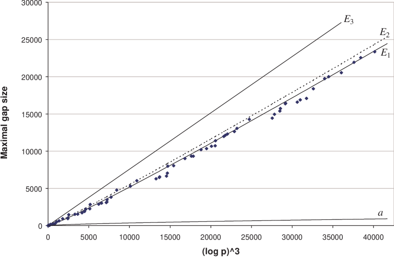
Figure 1: Maximal gaps between twin primes $\{p,p+2\}$ (A113274). Plotted (bottom to top): expected average gap $a=0.75739\log^{2}p$, estimators $E_{1}=a\log(p/a)-ba$, $E_{2}=a\log(p/a)$, $E_{3}=a\log p=0.75739\log^{3}p$, where $p$ is the end-of-gap prime; $b=1$.

Here are some observations suggested by these numerical results. (As before, $a$ denotes the expected average gap, $a=C_{k}\log^{k}p$, and $b={2\over k}$ unless stated otherwise.)

1. Estimators $E_{1}$ and $E_{2}$ overestimate some of the actual record gaps, but underestimate others. For $k\leq 6$, the data shows that $E_{1}$ is closer to a median-unbiased estimator. (We can make it even closer by tweaking the $b$ value; e. g., setting $b\approx 1.2597$ for twin primes, or $b\approx 0.7497$ for prime quadruplets, would turn $E_{1}$ into a median-unbiased estimator for maximal gaps below $10^{15}$.)

2. About 90% of the observed gaps are within $\pm 2a$ of the $E_{1}$ curve. Over 50% of the observed gaps are within $\pm a$ of $E_{1}$. This level of accuracy appears to be in line with heuristics based on statistical models (where the relevant extreme-value distributions have the standard deviation $\pi a/\sqrt{6}\approx 1.28a$; see Appendix).

3. Consider median-unbiased estimators $E_{\mbox{\tiny med}}(G_{k}(p))=a(\log(p/a)-b_{\mbox{\tiny med}})$ for $p<10^{15}$. Computations show that the value of $b_{\mbox{\tiny med}}$ tends to decrease when $k$ increases; also, our empirical value $b={2\over k}$ in the $E_{1}$ estimator is a little closer to zero than the median-unbiased value $b_{\mbox{\tiny med}}$. (For a simple way to refine $b$, see remark at the end of sect. 5.2.)

4. For relatively small values of $p$ that we deal with, the estimator $E_{3}$ may seem useless (too far above the realistic values). However, all three estimators are asymptotically equivalent, $E_{1}\sim E_{2}\sim E_{3}$ when $p\to\infty$.

5. The estimator $E_{3}=C_{k}\log^{k+1}p$ overestimates all known record gaps. In most cases, the error of $E_{3}$ is close to $a\log a$, exactly as expected from extreme-value statistics. Thus $E_{3}$ may be a good candidate for an upper bound for all record gaps; so in statement (B) of section 4.2 we may have $M_{k}=C_{k}=H_{k}^{-1}$, and

   $$G_{k}(p)<C_{k}\log^{k+1}p\qquad\mbox{(an analog of Cram\'{e}r's conjecture)}.$$

   It would be interesting to see any counterexamples, i. e., gaps exceeding $C_{k}\log^{k+1}p$.

   

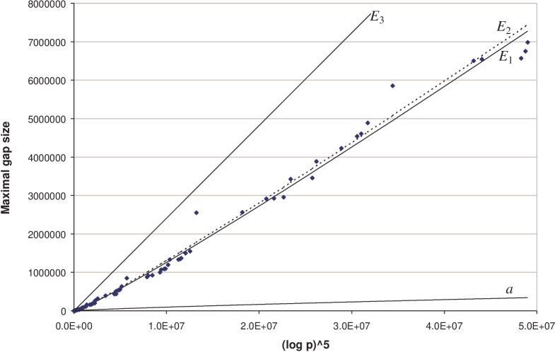
   Figure 2: Maximal gaps between prime quadruplets $\{p,p+2,p+6,p+8\}$ (A113404). Plotted (bottom to top): expected average gap $a=0.24089\log^{4}p$, estimators $E_{1}=a\log(p/a)-ba$, $E_{2}=a\log(p/a)$, $E_{3}=a\log p=0.24089\log^{5}p$, where $p$ is the end-of-gap prime; $b=1/2$.

Absolute error. The absolute error $|E_{i}-G_{k}(p)|$ tends to grow (but not monotonically) as $p\to\infty$ for all three estimators $E_{1}$, $E_{2}$, $E_{3}$. Heuristically, we expect the absolute error to be unbounded and, on average, continue to grow for all three estimators. Probable absolute errors are $O(a)$ for $E_{1}$ and $E_{2}$, and $O(a\log a)$ for $E_{3}$.

Relative error. The relative error $|\varepsilon_{i}|=|E_{i}-G_{k}(p)|/G_{k}(p)$ tends to decrease (but not monotonically) for all three estimators as $p\to\infty$. It may not be obvious from Figures 1–3, but we must have $|\varepsilon_{i}|\to 0$ either for all three estimators or for none of them. (Note: the limit of $|\varepsilon_{i}|$ as $p\to\infty$ might not exist at all; that would invalidate most of our conjectures.)

Error in average-gap units a. The error $(E_{3}-G_{k}(p))/a$, i. e., the $E_{3}$ error expressed as a number of expected average gaps, grows about as fast as $\log a$ (but not monotonically). Judging from limited numerical data, the corresponding error $(E_{i}-G_{k}(p))/a$ seems bounded as $p\to\infty$ if we use estimators $E_{1}$ or $E_{2}$. Heuristically, for $E_{1}$ and $E_{2}$ this error should remain bounded for the majority (but not all) of the record gaps.

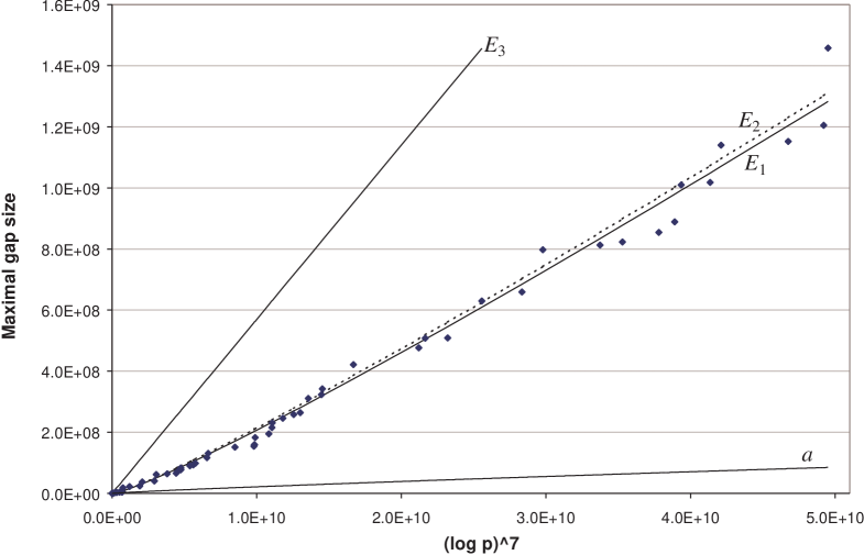
Figure 3: Maximal gaps between prime sextuplets $\{p$, $p+4$, $p+6$, $p+10$, $p+12$, $p+16\}$ (A200503). Plotted (bottom to top): expected average gap $a=0.057808\log^{6}p$, estimators $E_{1}=a\log(p/a)-ba$, $E_{2}=a\log(p/a)$, $E_{3}=a\log p=0.057808\log^{7}p$, where $p$ is the end-of-gap prime; $b=1/3$.

Overall, the prediction that record gaps are about $a\log(p/a)+O(a)$ appears correct for the vast majority of actual gaps, as far as we have checked ($p<10^{15}$). Note that the “optimal” $O(a)$ term ($-ba$ in the $E_{1}$ estimator) is negative, at least for $k\leq 6$. For larger values of $k$, the parameter $b$ gets closer to zero. Empirically, for $k$-tuples with $k\geq 6$, the $E_{1}$ estimator will likely produce good results even with $b\approx 0$. Therefore, for large $k$ we might want to simplify the model and use $b=0$, i. e., use the estimator $E_{2}=\max(a,a\log(p/a))$, the dotted curve in the above figure. However, maximal gap estimators with certain special properties (e.g., median-unbiased estimators) will still require nonzero values of $b$.

TABLE 2

Maximal gaps between twin primes $\{p$, $p+2\}$ below $10^{15}$

End-of-gap prime	Gap $g_{2}$	$g^{*}_{2}$ $1^{1}$	End-of-gap prime	Gap $g_{2}$	$g^{*}_{2}$ $1^{1}$
$1^{1}$ 5	2	0.084	24857585369	6552	$-2.765$
11	6	0.451	40253424707	6648	$-3.585$
29	12	0.180	42441722537	7050	$-2.811$
59	18	$-0.115$	43725670601	7980	$-0.830$
101	30	0.025	65095739789	8040	$-1.625$
347	36	$-1.205$	134037430661	8994	$-1.323$
419	72	$-0.112$	198311695061	9312	$-1.604$
809	150	1.247	223093069049	9318	$-1.865$
2549	168	$-0.396$	353503447439	10200	$-1.262$
6089	210	$-1.011$	484797813587	10338	$-1.747$
13679	282	$-1.189$	638432386859	10668	$-1.792$
18911	372	$-0.486$	784468525931	10710	$-2.195$
24917	498	0.645	794623910657	11388	$-1.032$
62927	630	0.290	1246446383771	11982	$-1.081$
188831	924	0.834	1344856603427	12138	$-0.998$
688451	930	$-1.728$	1496875698749	12288	$-1.002$
689459	1008	$-1.161$	2156652280241	12630	$-1.309$
851801	1452	1.577	2435613767159	13050	$-0.916$
2870471	1512	$-0.721$	4491437017589	14262	$-0.481$
4871441	1530	$-1.689$	13104143183687	14436	$-2.773$
9925709	1722	$-2.070$	14437327553219	14952	$-2.255$
14658419	1902	$-1.948$	18306891202907	15396	$-2.181$
17384669	2190	$-0.918$	18853633240931	15720	$-1.793$
30754487	2256	$-1.805$	23275487681261	16362	$-1.398$
32825201	2832	0.601	23634280603289	16422	$-1.351$
96896909	2868	$-1.646$	38533601847617	16590	$-2.291$
136286441	3012	$-1.812$	43697538408287	16896	$-2.178$
234970031	3102	$-2.611$	56484333994001	17082	$-2.539$
248644217	3180	$-2.451$	74668675834661	18384	$-1.507$
255953429	3480	$-1.454$	116741875918727	19746	$-0.864$
390821531	3804	$-1.260$	136391104748621	19992	$-0.940$
698547257	4770	0.571	221346439686641	20532	$-1.467$
2466646361	5292	$-0.816$	353971046725277	21930	$-0.955$
4289391551	6030	$-0.075$	450811253565767	22548	$-0.834$
19181742551	6282	$-2.831$	742914612279527	23358	$-1.149$
24215103971	6474	$-2.888$

TABLE 3

Maximal gaps between prime quadruplets $\{p$, $p+2$, $p+6$, $p+8\}$ below $10^{15}$

End-of-gap prime	Gap $g_{4}$	$g^{*}_{4}$ $1^{1}$	End-of-gap prime	Gap $g_{4}$	$g^{*}_{4}$ $1^{1}$
$1^{1}$ 11	6	0.430	3043668371	557340	$-0.750$
101	90	0.902	3593956781	635130	0.188
821	630	0.770	5676488561	846060	2.366
1481	660	0.192	25347516191	880530	$-1.576$
3251	1170	$-0.014$	27330084401	914250	$-1.358$
5651	2190	0.194	35644302761	922860	$-1.966$
9431	3780	0.518	56391153821	1004190	$-2.244$
31721	6420	$-0.125$	60369756611	1070490	$-1.697$
43781	8940	0.211	71336662541	1087410	$-1.967$
97841	9030	$-0.998$	76429066451	1093350	$-2.089$
135461	13260	$-0.539$	87996794651	1198260	$-1.383$
187631	16470	$-0.434$	96618108401	1336440	$-0.242$
326141	24150	$-0.094$	151024686971	1336470	$-1.535$
768191	28800	$-1.004$	164551739111	1348440	$-1.663$
1440581	29610	$-1.957$	171579255431	1370250	$-1.577$
1508621	39990	$-0.977$	211001269931	1499940	$-0.986$
3047411	56580	$-0.812$	260523870281	1550640	$-1.150$
3798071	56910	$-1.217$	342614346161	2550750	6.412
5146481	71610	$-0.714$	1970590230311	2561790	0.197
5610461	83460	$-0.049$	4231591019861	2915940	$-0.076$
9020981	94530	$-0.379$	5314238192771	2924040	$-0.748$
17301041	114450	$-0.678$	7002443749661	2955660	$-1.421$
22030271	157830	0.996	8547354997451	3422490	0.447
47774891	159060	$-0.861$	15114111476741	3456720	$-1.200$
66885851	171180	$-1.135$	16837637203481	3884670	0.533
76562021	177360	$-1.202$	30709979806601	4228350	0.134
87797861	190500	$-1.023$	43785656428091	4537920	0.307
122231111	197910	$-1.515$	47998985015621	4603410	0.278
132842111	268050	0.677	55341133421591	4884900	0.972
204651611	315840	1.022	92944033332041	5851320	2.995
628641701	395520	0.099	412724567171921	6499710	0.021
1749878981	435240	$-1.669$	473020896922661	6544740	$-0.293$
2115824561	440910	$-2.020$	885441684455891	6568590	$-2.253$
2128859981	513570	$-0.617$	947465694532961	6750330	$-1.932$
2625702551	536010	$-0.749$	979876644811451	6983730	$-1.356$
2933475731	539310	$-0.982$

Notes: Computing Tables 3 and 4 took the author two weeks on a quad-core 2.5 GHz CPU. Table 2 reflects Fischer’s extensive computation [5]. For earlier computations of maximal gaps by Boncompagni, Rodriguez, and Rivera, see OEIS A113274, A113404 [29], [26].

TABLE 4

Maximal gaps between prime 6-tuples $\{p$, $p+4$, $p+6$, $p+10$, $p+12$, $p+16\}$ below $10^{15}$

End-of-gap prime	Gap $g_{6}$	$g^{*}_{6}$ $1^{1}$	End-of-gap prime	Gap $g_{6}$	$g^{*}_{6}$ $1^{1}$
$1^{1}$ 97	90	1.856	422248594837	159663630	$-2.389$
16057	15960	1.414	427372467157	182378280	$-1.353$
43777	24360	0.949	610613084437	194658240	$-1.751$
1091257	1047480	1.570	660044815597	215261760	$-1.079$
6005887	2605680	1.176	661094353807	230683530	$-0.427$
14520547	2856000	$-0.048$	853878823867	245336910	$-0.573$
40660717	3605070	$-1.035$	1089869218717	258121710	$-0.786$
87423097	4438560	$-1.646$	1248116512537	263737740	$-0.968$
94752727	5268900	$-1.380$	1475318162947	311017980	0.246
112710877	17958150	3.778	1914657823357	322552230	$-0.170$
403629757	21955290	1.526	1954234803877	342447210	0.436
1593658597	23910600	$-1.149$	3428617938787	421877610	1.085
2057241997	37284660	0.730	9368397372277	475997340	$-0.740$
5933145847	40198200	$-1.318$	10255307592697	507945690	$-0.256$
6860027887	62438460	1.224	13787085608827	509301870	$-1.159$
14112464617	64094520	$-0.506$	21017344353277	629540730	0.084
23504713147	66134250	$-1.523$	33158448531067	659616720	$-0.819$
24720149677	70590030	$-1.228$	41349374379487	797025180	0.985
29715350377	77649390	$-1.038$	72703333384387	813158010	$-0.682$
29952516817	83360970	$-0.556$	89166606828697	823158840	$-1.190$
45645253597	90070470	$-1.064$	122421855415957	854569590	$-1.723$
53086708387	93143820	$-1.202$	139865086163977	888931050	$-1.642$
58528934197	98228130	$-1.063$	147694869231727	1010092650	$-0.077$
93495691687	117164040	$-0.935$	186010652137897	1018139850	$-0.755$
97367556817	131312160	$-0.108$	202608270995227	1139590200	0.603
240216429907	151078830	$-1.388$	332397997564807	1152229260	$-0.967$
414129003637	154904820	$-2.566$	424682861904937	1204960680	$-1.155$
419481585697	158654580	$-2.420$	437805730243237	1457965740	1.725

5.2 The distribution of maximal gaps

We have just seen that maximal gaps between prime $k$-tuples below $p$ grow about as fast as $a\log(p/a)$. Thus, the curve $a\log(p/a)$ (the dotted curve in Figures 1–3) may be regarded as a “trend.” Now we are going to take a closer look at the distribution of maximal gaps in the neighborhood of this “trend” curve. In our analysis, we will also include the case $k=1$, record gaps between primes (A005250). For each $k=1$, $2$, $4$, $6$, we will make a histogram of shifted and scaled (standardized) record gaps: subtract the “trend” $a\log(p/a)$ from actual gaps, and then divide the result by the “natural unit” $a$, the expected average gap. This way, all record gaps $g_{k}(p)$ are mapped to standardized values $g_{k}^{*}$ (shown in Tables 2–4):

$$g_{k}(p)~{}~{}\to~{}~{}g_{k}^{*}=\frac{g_{k}(p)-a\log(p/a)}{a},\quad\mbox{ where~{} }a=C_{k}\log^{k}p.$$

Record gaps that exceed $a\log(p/a)$ are mapped to standardized values $g_{k}^{*}>0$, while those below $a\log(p/a)$ are mapped to $g_{k}^{*}<0$. Note that the majority of known record gaps are below the dotted curve in Figures 1–3; accordingly, most of the standardized values $g_{k}^{*}$ are negative. It is also immediately apparent that the histograms and fitting distributions are skewed: the right tail is longer and heavier. This skewness is a well-known characteristic of extreme value distributions — and it comes as no surprise that a good fit obtained with the help of distribution-fitting software [21] is the Gumbel distribution, a common type of extreme value distribution (see Appendix).

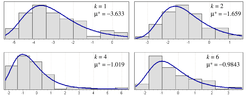
Figure 4: The distribution of standardized maximal gaps $g_{k}^{*}$: histograms and the fitting Gumbel distribution PDFs. For $k=1$ (primes), the histogram shows record gaps below $4\times 10^{18}$. For $k=2,4,6$ ($k$-tuples), the histograms show record gaps below $10^{15}$.

Here is why we can say that the Gumbel distribution is indeed a good fit:

(1) Based on goodness-of-fit statistics (the Anderson-Darling test as well as the Kolmogorov-Smirnov test), one cannot reject the hypothesis that the standardized values $g_{k}^{*}$ might be values of independent identically distributed random variables with the Gumbel distribution.

(2) Although a few other distributions could not be rejected either, the Anderson-Darling and Kolmogorov-Smirnov goodness-of-fit statistics for the Gumbel distribution are better than the respective statistics for any other two-parameter distribution we tried (including normal, uniform, logistic, Laplace, Cauchy, power-law, etc.), and better than for several three-parameter distributions (e. g., triangular, error, Beta-PERT, and others).

An equally good or even marginally better fit is the three-parameter generalized extreme value (GEV) distribution, which in fact includes the Gumbel distribution as a special case. The shape parameter in the fitted GEV distribution turns out very close to zero; note that a GEV distribution with a zero shape parameter is precisely the Gumbel distribution. The scale parameter of the fitted Gumbel distribution is close to one. The mode $\mu^{*}$ of the fitted distribution is negative. Figure 4 gives the approximate value of $\mu^{*}$ for $k=1,2,4,6$; $\mu^{*}$ is the coordinate of the maximum of the distribution PDF (probability density function).

Note: Now that we have a more precise value of the mode $\mu^{*}$, we can refine the parameter $b$ in the $E_{1}$ estimator: use $-b=\mu^{*}+\gamma$, which estimates the mean of the fitted Gumbel distribution in Fig. 4. Here $\gamma=0.5772...$ is the Euler-Mascheroni constant.

6 On maximal gaps between primes

Let us now apply our model of gaps to maximal gaps between primes (A005250) [29], [23]:

Maximal prime gaps are about $a\log(p/a)-ba$, with $a=\log p$ and $b\approx 3$.

If all record gaps behave like those in Figure 5 (showing the 75 known record gaps between primes $p<4\times 10^{18}$), this would confirm the Cramér and Shanks conjectures: maximal prime gaps are smaller than $\log^{2}p$ — but smaller only by $O(a\log a)$. We also easily see that the Cramér and Shanks conjectures are compatible with our estimate of record gaps. Indeed, for $a=\log p$ and any fixed $b\geq 0$, we have $\log^{2}p\sim a(\log(p/a)-b)<\log^{2}p$ as $p\to\infty$.

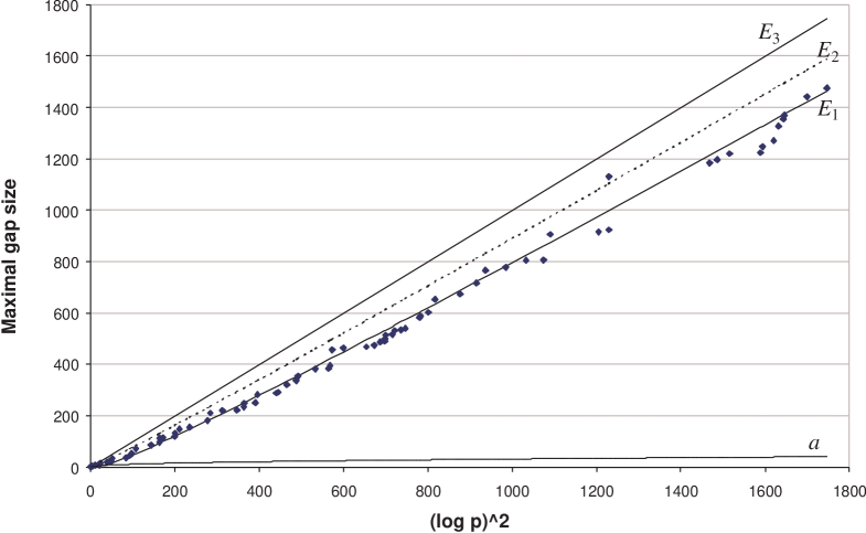
Figure 5: Maximal gaps between consecutive primes (A005250). Plotted (bottom to top): expected average gap $a=\log p$, estimators $E_{1}=a\log(p/a)-ba$, $E_{2}=a\log(p/a)$ (dotted), $E_{3}=a\log p=\log^{2}p$, where $p$ is the end-of-gap prime; $b=3$.

Notes: Maier’s theorem (1985) [19] states that there are (relatively short) intervals where typical gaps between primes are greater than the average ($\log p$) expected from the prime number theorem. Based in part on Maier’s theorem, Granville [12] adjusted the Cramér conjecture and proposed that, as $p\to\infty$, $\lim\sup(G(p)/\log^{2}p)\geq 2e^{-\gamma}=1.1229\ldots$ This would mean that an infinite subsequence of maximal gaps must lie above the Cramér-Shanks upper limit $\log^{2}p$, i. e., above the $E_{3}$ line in Figure 5 — and this hypothetical subsequence (or an infinite subset thereof) must approach a line whose slope is about 1.1229 times steeper! However, for now, there are no known maximal prime gaps above $\log^{2}p$. Interestingly, Maier himself did not voice serious concerns that the Cramér or Shanks conjecture might be in danger because of his theorem; thus, Maier and Pomerance [20] simply remarked in 1990:

Cramér conjectured that $\lim\sup G(x)/\log^{2}\negthinspace x=1$, while Shanks made the stronger conjecture that $G(x)\sim\log^{2}x$, but we are still a long way from proving these statements.

7 Corollaries: Legendre-type conjectures

Assuming the conjectures of Section 4, one can state (and verify with the aid of a computer) a number of interesting corollaries. The following conjectures generalize Legendre’s conjecture about primes between squares.

• For each integer $n>0$, there is always a prime between $n^{2}$ and $(n+1)^{2}$. (Legendre)

• For each integer $n>122$, there are twin primes between $n^{2}$ and $(n+1)^{2}$. (A091592)

• For each integer $n>3113$, there is a prime triplet between $n^{2}$ and $(n+1)^{2}$.

• For each integer $n>719377$, there is a prime quadruplet between $n^{2}$ and $(n+1)^{2}$.

• For each integer $n>15467683$, there is a prime quintuplet between $n^{2}$ and $(n+1)^{2}$.

• There exists a sequence $\{s_{k}\}$ such that, for each integer $n>s_{k}$, there is a prime $k$-tuplet between $n^{2}$ and $(n+1)^{2}$. (This $\{s_{k}\}$ is OEIS A192870: $0,122,3113,719377,\ldots$)

Another family of Legendre-type conjectures for prime $k$-tuplets can be obtained by replacing squares with cubes, 4th, 5th, and higher powers of $n$:

• For each integer $n>0$, there are twin primes between $n^{3}$ and $(n+1)^{3}$.

• For each integer $n>0$, there is a prime triplet between $n^{4}$ and $(n+1)^{4}$.

• For each integer $n>0$, there is a prime quadruplet between $n^{5}$ and $(n+1)^{5}$.

• For each integer $n>0$, there is a prime quintuplet between $n^{6}$ and $(n+1)^{6}$.

• For each integer $n>6$, there is a prime sextuplet between $n^{7}$ and $(n+1)^{7}$.

A further generalization is also possible:

• There is a prime $k$-tuplet between $n^{r}$ and $(n+1)^{r}$ for each integer $n>n_{0}(k,r)$, where $n_{0}(k,r)$ is a function of $k\geq 1$ and $r>1$.

To justify the above Legendre-type conjectures, we can assume the $k$-tuple conjecture plus statement (B) (sect. 4.2) bounding the size of gaps between $k$-tuples: $g_{k}(p)<M_{k}\log^{k+1}p$. We can now use the following elementary argument: Consider a fixed $r>1$, and let $x$ be a number in the interval between $n^{r}$ and $(n+1)^{r}$. Then, for large $n$, the interval size $d_{r}=(n+1)^{r}-n^{r}\sim rn^{r-1}$ will be asymptotic to $rx^{(r-1)/r}$: because $x\sim n^{r}$ and $d_{r}\sim rn^{r-1}$ when $n\to\infty$, we have $n\sim x^{1/r}$ and $d_{r}\sim rx^{(r-1)/r}$ when $x\to\infty$. But any positive power of $x$ grows faster than any positive power of $\log x$ when $x\to\infty$. So $x^{(r-1)/r}$ must grow faster than $\log^{k+1}x$. Therefore, the intervals $[n^{r},(n+1)^{r}]$ — whose sizes are about $rx^{(r-1)/r}$ — will eventually become much larger than the largest gaps between prime $k$-tuples containing primes $p\approx x$. For smaller $n$, a computer check finishes the job.

However, this is not a proof: we have relied on unproven assumptions. As Hardy and Wright pointed out in 1938 (referring to the infinitude of twin primes and prime triplets),

Such conjectures, with larger sets of primes, can be multiplied, but their proof or disproof is at present beyond the resources of mathematics. [15, p. 6]

Many years have passed, yet conjectures like these remain exceedingly difficult to prove.

8 Appendix: a note on statistics of extremes

In this appendix we use extreme value statistics to derive a simple formula expressing the expected maximal interval between rare random events in terms of the average interval:

$$E(\mbox{max interval})=a\log(T/a)+O(a)\qquad\qquad(1\ll a\ll T),$$

where $a$ is the average interval between the rare events, $T$ is the total observation time or length, as applicable, and $E(\mbox{max interval})$ stands for the mathematical expectation of the maximal interval. The formula holds for random events occurring at exponentially distributed (real-valued) intervals, as well as for events occurring at geometrically distributed discrete (integer-valued) intervals. (For more information on extreme value distributions of random sequences see Gumbel’s classical book [13] or more recent books [1], [9]. For extreme value distributions of discrete random sequences, such as head runs in coin toss sequences, see also the papers of Schilling [27] or Gordon, Schilling, and Waterman [11] and further references therein.)

8.1 Two problems about random events

For illustration purposes, we will use two problems:

Problem A. Consider a non-stop toll bridge with very light traffic. Let $P>1/2$ be the probability that no car crosses the toll line during a one-second interval, and $q=1-P$ the probability to see a car at the toll line during any given second. Suppose we observe the bridge for a total of $T$ seconds, where $T$ is large, while $P$ is constant.

Problem B. Consider a biased coin with a probability of heads $P>1/2$ (and the probability of tails $q=1-P$). We toss the coin a total of $T$ times, where $T$ is large.

In both problems, answer the following questions about the rare events (cars or tails):

(1) What is the expected total number of rare events in the observation series of length $T$?

(2) What is the expected average interval $a$ between events (i. e., between cars/tails)?

(3) What is the expected maximal interval between events, as a function of $a$?

Notice that the first two questions are much easier than the third. Here are the easy answers:

(1) Because the probability of the event is $q$ at any given second/toss, we expect a total of $nq$ events after $n$ seconds/tosses, and a total of $Tq$ events at the end of the entire observation series of length $T$.

(2) To estimate the expected average interval $a$ between events, we divide the total length $T$ of our observation series by the expected total number of events $Tq$. So a reasonable estimate of the expected average interval between events is $a\approx T/(Tq)=1/q$.

(3) Quite obviously, we can predict that the expected maximal interval is less than $T$, but not less than $a$:

$$a\leq E(\mbox{max interval})<T.$$

The expected maximal interval will likely depend on both $a$ and $T$:

$$E(\mbox{max interval})=f(a,T).$$

It is also reasonable to expect that $f(a,T)$ should be an increasing function of both arguments, $a$ and $T$. Can we say anything more specific about the expected maximal interval?

8.2 An estimate of the most probable maximal interval

In both problems A and B we will assume that $1\ll a\ll T$ — or, in plain English:

• the events are rare ($1\ll a$), and

• our observations continue for long enough to see many events ($a\ll T$).

In Problem A, to estimate the most probable maximal interval between cars we proceed as follows: After $n$ seconds of observations, we would have seen about $nq$ cars, hence about $nq$ intervals between cars. The intervals are independent of each other and real-valued. A known good model for the distribution of these intervals is the exponential distribution that has the cumulative distribution function (CDF) $1-P^{\,t}$:

with probability $P$, any given interval between cars is at least 1 second;

with probability $P^{2}$, any given interval is at least 2 seconds;

with probability $P^{3}$, any given interval is at least 3 seconds;$\ldots$

with probability $P^{\,t}$, any given interval is at least $t$ seconds.

Thus, after $n$ seconds of observations and about $nq$ carless intervals, we would reasonably expect that at least one interval is no shorter than $t$ seconds if we choose $t$ such that

$$P^{\,t}\times(nq)\geq 1.$$

Now it is easy to estimate the most probable maximal interval $t_{\max}$:

$$P^{\,t_{\max}}\approx 1/(nq)$$

$$(1/P)^{t_{\max}}\approx nq$$

$$t_{\max}\approx\log_{1/P}(nq).$$

In Problem B we can estimate the longest run of heads $R_{n}$ after $n$ coin tosses reasoning very similarly. One notable difference is that now the head runs are discrete (have integer lengths). Accordingly, they are modeled using the geometric distribution. Schilling [27] has this estimate for the longest run of heads after $n$ tosses, given the heads probability $P$:

$$R_{n}\approx\log_{1/P}(nq).$$

In both problems, the estimates for the most probable maximal interval (as a function of $P$ and $n$) have the same form $\log_{1/P}(nq)$. Therefore, it is reasonable to expect that the answers to our original question (3) in both problems A and B will also be the same or similar functions of the average interval $a$, even though the problems are modeled using different distributions of intervals. We will soon see that this indeed is the case.

8.3 If random events are rare…

If the events (cars in Problem A, or tails in Problem B) are rare, then $P$ is close to 1, and $q$ is close to 0. Using the Taylor series expansion of $\log(1/(1-q))$, we can write:

$$\log(1/P)=\log\left({1\over{1-q}}\right)=q+{q^{2}\over 2}+{q^{3}\over 3}+\ldots=q+O(q^{2})$$

or, omitting the $O(q^{2})$ terms,

$$\log(1/P) \approx q,\qquad\qquad\mbox{ and therefore }$$

$${1\over\log(1/P)} \approx {1\over q}~{}\approx~{}a\qquad(\mbox{moreover, we have }{1\over\log(1/P)}=a\mbox{ \,in Problem A}).$$

So we can transform the estimate of most probable maximal intervals, $\log_{1/P}(nq)$, like this:

$$\log_{1/P}(nq)=\log(nq)/\log(1/P)\approx(1/q)\log(nq)\approx a\log(n/a).$$

For a long series of observations, with the total length or duration $n=T$ (e. g. $T$ tosses of a biased coin, or $T$ seconds of observing the bridge), the estimate for the most probable maximal interval becomes $a\log(T/a)$.

8.4 Expected maximal intervals

The specific formulas for expected maximal intervals between rare events depend on the nature of events in the problem (whether the initial distribution of intervals is exponential or geometric). However, as $T\to\infty$, in the formulas for both cases the highest-order term turns out to be the same: $a\log(T/a)$, which was precisely our estimate for the most probable maximal interval.

(A) Exponential initial distribution. Fisher and Tippett [7], Gnedenko [10], Gumbel [13] and other authors showed that, for initial distributions of exponential type (including, as a special case, the exponential distribution) the limiting distribution of maximal terms in a random sequence is the double exponential distribution — often called the Gumbel distribution. In particular, if intervals between cars in Problem A have exponential distribution with CDF $1-P^{\,t}=1-e^{-t/a}$, then the distribution of maximal intervals has these characteristics:

$$N (1-e^{-t/a})^{N}=(1-\textstyle{1\over N}e^{-(t-\mu_{N})/a})^{N}\quad\mbox{(distribution for $N\approx Tq$ events), }$$-event CDF:

Limiting CDF: $$\exp(-e^{-(t-\mu)/a})\qquad\mbox{(Gumbel distribution) \cite[cite]{[\@@bibref{}{gumbel}{}{}, \rm p.\,157]},}$$

Scale $$= a~{}=~{}1/\log(1/P)\quad\mbox{ (equal to the expected average interval)},$$

Mode $$= \mu~{}=~{}\mu_{N}~{}=~{}a\log N~{}\approx~{}a\log(T/a)~{}\approx~{}\log_{1/P}(Tq),$$

Median $$= \mu-a\log\log 2~{}\approx~{}a\log(T/a)+0.3665a,$$

Mean $$= \mu+\gamma a~{}\approx~{}a\log(T/a)+0.5772a,$$

where $\gamma=0.5772...$ is the Euler-Mascheroni constant. The mean value of observed maximal intervals in Problem A will converge almost surely to the mean $\mu+a\gamma$ of the Gumbel distribution, therefore:

$$E(\mbox{max interval})~{}\approx~{}\log_{1/P}(Tq)+\gamma a~{}\approx~{}a\log(T/a)+\gamma a~{}=~{}a\log(T/a)+O(a).$$

Historical notes: In 1928 Fisher and Tippett [7] described three types of limiting extreme-value distributions and showed that the double exponential (Gumbel) distribution is the limiting extreme-value distribution for a certain wide class of random sequences. They also computed, among other parameters, the mean-to-mode distance in the double exponential distribution [7, p. 186]; it is this result that allows one to conclude that the mean is $\mu+a\gamma$ if the mode is $\mu$. Gnedenko (1943) [10] rigorously proved the necessary and sufficient conditions for an initial distribution to be in the domain of attraction of a given type of limiting distribution.

(B) Geometric initial distribution. Surprisingly, in this case the limiting extreme-value distribution does not exist [27, p. 203], [11, p. 280]. For the longest run of heads $R_{n}$ in a series of $n$ tosses of a biased coin, with the probability of heads $P$, we have

$$E(R_{n})=\log_{1/P}(nq)+\frac{\gamma}{\log(1/P)}-{1\over 2}+\mbox{smaller terms}\qquad\mbox{\cite[cite]{[\@@bibref{}{schilling}{}{}, \rm p.\,202]}},$$

where the first term is the same as in Problem A (up to a substitution $n=T$). The sum of the other terms is $O(a)$ when $P$ is close to 1; so, again, we have

$$E(R_{n})=a\log(n/a)+O(a).$$

8.5 Standard deviation of extremes

As above, the specific formula for standard deviation (SD) in distributions of maximal intervals between events depends on the nature of the problem (whether the initial distribution of intervals is exponential or geometric). Still, in both cases SD $\approx\pi a/\sqrt{6}=O(a)$.

(A) Exponential initial distribution. Here the limiting distribution of maximal intervals is the Gumbel distribution with the scale $a=1/\log(1/P)$, therefore the SD of maximal intervals must be very close to the SD of the Gumbel distribution:

$$\mbox{SD}(\mbox{max interval})\approx{\pi a\over\sqrt{6}}=O(a)\qquad\mbox{\cite[cite]{[\@@bibref{}{gumbel}{}{}, \rm p.\,116,\,174]}}.$$

(B) Geometric initial distribution. For the longest run of heads $R_{n}$ in a series of $n$ tosses of a biased coin, the variance is

$$\mbox{Var\,}R_{n}={\pi^{2}\over 6\log^{2}(1/P)}+{1\over 12}+\mbox{smaller terms}\qquad\mbox{\cite[cite]{[\@@bibref{}{schilling}{}{}, \rm p.\,202]}},$$

where the first term is $O(a^{2})$, while the sum of the other terms is much smaller than the first term. (Again, recall that for average intervals $a$ between rare events — in this case, between tails — we have $a\approx 1/\log(1/P)$.) Therefore, the standard deviation is

$$\mbox{SD}\,\,R_{n}=\sqrt{\mbox{Var\,}R_{n}}={\pi\over\sqrt{6}\log(1/P)}+\mbox{a small term}\approx{\pi a\over\sqrt{6}}=O(a).$$

8.6 A shortcut to the answer

There is a simple way to “guesstimate” the answer $a\log(T/a)+O(a)$. If $a$ is the average interval between events, then the most probable maximal interval is about $a\log(T/a)$ (sect. 8.3). We can now simply use the fact that the width of the extreme value distribution is $O(a)$. (Imagine what happens if the rare event’s probability $q$ is reduced by 50%. This change in $q$ would have about the same effect as if every interval became twice as large: then average and maximal intervals would also become twice as large, and the extreme value distribution would be twice as wide. This immediately implies that the extreme value distribution is $O(a)$ wide.) But then the true value of the expected maximal interval cannot be any farther than $O(a)$ from our estimate $a\log(T/a)$; so the expected maximal interval is $a\log(T/a)+O(a)$.

8.7 Summary

We have considered maximal intervals between random events in two common situations:

• rare events occurring at exponentially distributed intervals (Problem A);

• discrete rare events at geometrically distributed intervals (Problem B).

These two situations are somewhat different: in the former case maximal intervals have a limiting distribution (the Gumbel distribution), while in the latter case no limiting distribution exists (here the Gumbel distribution is simply a decent approximation). Nevertheless, in both cases the expected maximal interval between events is

$$E(\mbox{max interval})=a\log(T/a)+\gamma a+\mbox{lower-order terms }=a\log(T/a)+O(a),$$

where $a$ is the average interval between events, $T$ is the total observation time or length, and the lower-order terms depend on the initial distribution.

As we have seen in Sections 4–6, a remarkably similar heuristic formula $a\log(x/a)-ba$, with an empirical term $-ba$ replacing the “theoretical” $\gamma a$, satisfactorily describes the following:

• record gaps between primes below $x$ ($a=\log x$, $b\approx 3$; A005250)

• record gaps between twin primes below $x$ ($a=0.75739\log^{2}x$, $b\approx 1$; A113274) and, more generally,

• record gaps between prime $k$-tuples ($a=C_{k}\log^{k}x$, $b\approx 2/k$, where $C_{k}$ is reciprocal to the Hardy-Littlewood constant for the particular $k$-tuple).

9 Acknowledgements

The author is grateful to the anonymous referee and to all authors, contributors, and editors of the websites OEIS.org, PrimePuzzles.net and FermatQuotient.com. Many thanks also to Prof. Marek Wolf for his interest in the initial version of this paper, followed by an email exchange that undoubtedly helped make this paper better.

 

2010 Mathematics Subject Classification: Primary 11N05; Secondary 60G70.

Keywords: distribution of primes, prime $k$-tuple, Hardy-Littlewood conjecture, extreme value statistics, Gumbel distribution, prime gap, Cramér conjecture, prime constellation, twin prime conjecture, prime quadruplet, prime sextuplet.

 

(Concerned with OEIS sequences A005250, A091592, A113274, A113404, A192870, A200503, A201596, A201598, A201051, A201062, A201073, A201251, A202281, A202361.)

References

- [1] J. Beirlant, Y. Goegebeur, J. Segers and J. Teugels, Statistics of Extremes: Theory and Applications, Wiley, 2004.
- [2] S. M. Berman, Limiting distributions of the maximum term in sequences of dependent random variables. Annals of Mathematical Statistics, 33 (1962), 894–908.
- [3] H. Cohen, High precision computation of Hardy-Littlewood constants, preprint. http://www.math.u-bordeaux1.fr/~cohen/hardylw.dvi (2012).
- [4] H. Cramér, On the order of magnitude of the difference between consecutive prime numbers. Acta Arith. 2 (1937), 23–46.
- [5] R. Fischer, Maximale Lücken (Intervallen) von Primzahlenzwillingen, web page (in German) http://www.fermatquotient.com/PrimLuecken/ZwillingsRekordLuecken (2008).
- [6] R. Fischer, Maximale Intervalle von Primzahlenpaaren, web page (in German). Maximal gaps between twin primes are . Maximal gaps between prime triplets are . http://www.fermatquotient.com/PrimLuecken/Max_Intervalle (2006).
- [7] R. A. Fisher and L. H. C. Tippett, Limiting forms of the frequency distribution of the largest and smallest member of a sample, Proc. Camb. Phil. Soc., 24 (1928), 180–190.
- [8] A. D. Forbes, Prime -tuplets. Section 21: List of all possible patterns of prime -tuplets. The Hardy-Littlewood constants pertaining to the distribution of prime -tuplets. http://anthony.d.forbes.googlepages.com/ktuplets.htm (2012).
- [9] J. Galambos, The Asymptotic Theory of Extreme Order Statistics, Krieger, 1987.
- [10] B. V. Gnedenko, Sur la distribution limite du terme maximum d’une série aléatoire. Ann. Math., 44 (1943), 423–453. (English translation: On the limiting distribution of the maximum term in a random series. Breakthroughs in Statistics, Volume 1: Foundations and Basic Theory. Springer, New York, 1993, pp. 185–225.)
- [11] L. Gordon, M. F. Schilling, and M. S. Waterman, An extreme value theory for long head runs. Probability Theory and Related Fields, 72 (1986), 279–297.
- [12] A. Granville. Harald Cramér and the distribution of prime numbers. Scand. Act. J., 1 (1995), 12–28.
- [13] E. J. Gumbel, Statistics of Extremes, Columbia University Press, 1958. Dover, 2004.
- [14] G. H. Hardy and J. E. Littlewood, Some Problems of ‘Partitio Numerorum.’ III. On the Expression of a Number as a Sum of Primes. Acta Math. 44 (1922), 1–70.
- [15] G. H. Hardy and E. M. Wright, An Introduction to the Theory of Numbers, 6th ed. Oxford University Press, 2008.
- [16] W. L. Hays, Statistics, Harcourt Brace College Publishers, 1994.
- [17] P. F. Kelly and T. Pilling, Implications of a new characterisation of the distribution of twin primes. http://arxiv.org/abs/math/0104205 (2001).
- [18] P. F. Kelly and T. Pilling, Physically inspired analysis of prime number constellations. http://arxiv.org/abs/hep-th/0108241 (2001).
- [19] H. Maier, Primes in short intervals, Michigan Math. J., 32 (1985), 221–225.
- [20] H. Maier and C. Pomerance, Unusually large gaps between consecutive primes. Transactions of the AMS, 322 (1990), 201–237.
- [21] MathWave Technologies, EasyFit — Distribution Fitting Software, the company web site at http://www.mathwave.com/easyfit-distribution-fitting.html (2012).
- [22] Microsoft Corporation, Excel: Add a Trendline to a Chart, the company web site at http://office.microsoft.com/en-us/excel-help/add-a-trendline-to-a-chart-HP005198462.aspx (2012).
- [23] T. R. Nicely, List of prime gaps. http://www.trnicely.net/gaps/gaplist.html (2012).
- [24] J. Pintz, Cramér vs Cramér: On Cramér’s probabilistic model of primes. Functiones et Approximatio, XXXVII.2 (2007), 361–376.
- [25] H. Riesel, Prime Numbers and Computer Methods for Factorization, Birkhäuser, 1994.
- [26] L. Rodriguez and C. Rivera, Conjecture 66. Gaps between consecutive twin prime pairs. http://www.primepuzzles.net/conjectures/conj_066.htm (2009).
- [27] M. F. Schilling, The longest run of heads. The College Math. J., 21 (1990), 196–207.
- [28] D. Shanks, On maximal gaps between successive primes. Math. Comput. 18 (1964), 646–651.
- [29] N. J. A. Sloane, On-Line Encyclopedia of Integer Sequences, http://oeis.org (2012).
- [30] G. S. Watson, Extreme values in samples from -dependent stationary stochastic processes. Annals of Mathematical Statistics, 25 (1954), 798–800.
- [31] M. Wolf, Some heuristics on the gaps between consecutive primes, arXiv preprint. http://arxiv.org/abs/1102.0481 (2011)
- [32] M. Wolf, Maximal gaps between twin primes can be expressed in terms of . E-mail communication (2013).