New Colour—Mass to Light Relations: the role of the Asymptotic Giant Branch phase and of interstellar dust

Abstract

Colour-$M_{\star}/L$ (mass–to–light) relations are a popular recipe to derive stellar mass in external galaxies. Stellar mass estimates often rely on near infrared (NIR) photometry, considered an optimal tracer since it is little affected by dust and by the ”frosting” effect of recent star formation episodes. However, recent literature has highlighted that theoretical estimates of the NIR $M_{\star}/L$ ratio strongly depend on the modelling of the Asymptotic Giant Branch (AGB) phase.

We use the latest Padova isochrones, with detailed modelling of the Thermally Pulsing AGB phase, to update theoretical colour-$M_{\star}/L$ relations in the optical and NIR and discuss the consequences for the estimated stellar masses in external galaxies.

We also discuss the effect of attenuation by interstellar dust on colour-$M_{\star}/L$ relations in the statistical case of large galaxy samples.

1 Introduction

Various astrophysical problems require to estimate stellar mass from the photometry: for instance, to reconstruct the assembly history of galaxies through cosmic times (e.g. Bell et al., 2003, 2004) ; to define the stellar/baryonic mass Tully–Fisher relation, which is more physically meaningful than in any specific photometric band (Bell & de Jong, 2001; McGaugh, 2005); to determine the inventory of baryons in the Universe (Fukugita, Hogan & Peebles 1998; Fukugita & Peebles 2004; McGaugh et al. 2010); and to disentangle the contribution of luminous versus dark matter in galactic dynamics (e.g. Portinari & Salucci, 2010, and references therein).

The key to it is the stellar mass–to–light ratio ($M_{\star}/L$). For a Simple Stellar Population (ensemble of coeval stars with the same chemical composition, formed in the same burst of star formation), $M_{\star}/L$ depends on (a) the Initial Mass Function; (b) the age and (c) the metallicity.; for a composite stellar population, (b) and (c) become, respectively, age distribution (star formation history) and metallicity distribution. Population synthesis techniques and chemo-photometric models of galaxies can predict theoretical $M_{\star}/L$ ratios (including both living stars and remnants) associated to the photometric properties; yet only in the past decade this possibility has been fully appreciated in the dynamical and extra-galactic community. In particular, colour—$M_{\star}/L$ relations have become a popular and handy tool to estimate stellar masses in external galaxies (e.g. Kranz, Slyz & Rix 2003; McGaugh 2004; Kassin, de Jong & Weiner 2006; Bakos, Trujillo & Pohlen 2008; Treuthard, Salo & Buta 2009; Torres-Flores et al. 2011).

Early on, Sargent & Tinsley (1974) and Larson & Tinsley (1978) reported tight relations between colour and $M_{\star}/L$ for $B,V$ bands, used by Tinsley (1981) to discuss the dark matter content in galaxies of different Hubble type. Those papers presented the first linear equation relating colour and log($M_{\star}/L$), and the insightful remark that, adopting a different Initial Mass Function (IMF) “All the models of a set could be arbitrarily moved up or down in $\log M/L_{B}$ […] The slopes of the relations would not be altered”.

After the pioneering papers of Tinsley and collaborators, the next analysis of $M_{\star}/L$ ratios from galactic models was by Jablonka & Arimoto (1992), who extended colour–$M_{\star}/L$ relations to near infrared (NIR) bands; it is of historical interest that, in those early models, the $M_{\star}/L_{H}$ vs. $(B-H)$ relation had a negative slope, at odds with relations in optical bands. Their models were used by Persic et al. (1993) to discuss the dark matter content of galaxies as a function of luminosity.

These early results on $M_{\star}/L$ from galactic models went otherwise mostly unnoticed. The breakthrough introduction of “colour–$M_{\star}/L$ relations” to the wider dynamical and extra-galactic community, was the extensive study of Bell & de Jong (2001): they showed that a variety of disc galaxy models (closed box models, open models with inflows or outflows, with different formation age, with starbursts, etc.) all resulted in the same, robust log–linear colour–$M_{\star}/L$ relations (CMLR). The tightest relations involve optical bands, where the notorious age–metallicity degeneracy is, for once, an advantage, as it concurs to keeping the relation tight. Similar CMLR were found to hold within disc galaxy models, along the radial colour profiles obtained in the inside–out scenario (Portinari, Sommer-Larsen & Tantalo, 2004). Semi–empirical (as opposed to purely theoretical) CMLR have been derived by Bell et al. (2003) from multi-band photometry of galaxies in the SDSS+2MASS surveys.

A key feature of CMLR, also highlighted by Bell & de Jong (2001), is that the zero–point of the relation is set by the stellar IMF, while the slope of the relation is robust versus this, and other, model assumptions. The zero–point in the optical bands ($B,V,I$) seems to be well established (Flynn et al., 2006): models of the local Galactic disc based on star counts yield a colour–$M_{\star}/L$ datapoint for the “solar cylinder” that agrees with the normalization of typical Solar Neighbourhood IMFs (Kroupa, 1998; Chabrier, 2001, 2002).

To estimate stellar mass, near infrared (NIR) photometry is most often a favoured choice: (i) NIR luminosity, less affected than optical bands by minor recent star formation episodes (the “frosting” effect), is a better tracer of the bulk of the stellar population. (ii) The $M_{\star}/L$ ratio in the NIR varies, overall, less than in the optical (Bell & de Jong, 2001) — though it is not constant and totally insensitive to the star formation history, as often assumed in the past. (iii) NIR luminosity is less affected by dust extinction. (iv) Nowadays NIR studies benefit from excellent large databases obtained from extensive surveys (2MASS, UKIDSS, etc.)

However, the integrated NIR light of a stellar population is heavily affected by the contribution of its Asymptotic Giant Branch (AGB) stars (Maraston, 1998, 2005; Girardi & Bertelli, 1998; Mouhcine & Lançon, 2002, 2003). At intermediate ages (0.3–3 Gyr) the AGB phase dominates the NIR emission, lowering the K–band $M_{\star}/L$ ratio by a factor of 3–5 and inducing a colour transition to the red, reaching $(V-K)\geq 3$. For high redshift galaxies in the relevant age range ($z\sim 2$, ages 0.2–2 Gyr), population synthesis models including the AGB phase yield about 1 mag brighter K–band luminosities, 2 mag redder $(V-K)$ colours, and 60% lower stellar masses and ages than other models (Maraston, 2006; Tonini et al., 2009).

It is by now well established that, in spite of its short–lived nature, the complex Thermally Pulsing (TP)-AGB phase has considerable impact on NIR colours and $M_{\star}/L$, and needs to be accurately modelled. Major advances in this respect have been implemented in the recent release of the Padova isochrones. In this paper, we explore their consequences on theoretical CMLR.

The paper is organized as follows. In Section 2 we discuss CMLR for Simple Stellar Populations, comparing the previous and recent release of the Padova isochrones, differing only in the TP-AGB phase implementation. In Section 3 we derive CMLR for composite stellar populations resulting from extended star formation histories. In Section 4 we derive CMLR for more detailed disc galaxy models with internal colour and metallicity gradients (Portinari et al., 2004).

Dust can also influence CMLR relations, although to first order approximation, it is believed to have little impact on optical CMLR, as the dust extinction+reddening vector runs almost parallel to the CMLR itself (Bell & de Jong, 2001). The past decade saw major progress in modelling the effects of interstellar dust on the integrated light of galaxies (e.g. Silva et al., 1998; Popescu et al., 2000; Piovan et al., 2006). We therefore revisit the role of dust on CMLR by including the attenuation effects derived from detailed radiative transfer models (Tuffs et al., 2004). Section 5 is thus dedicated to the CMLR of (normal) dusty galaxies. In Section 6 we outline our summary and conclusions.

2 Colour–$M_{\star}/L$ relations for Simple Stellar Populations

In this section we discuss CMLR for Simple Stellar Populations (SSPs; Renzini & Buzzoni, 1986). We analyze the role of the TP-AGB phase by comparing SSPs based on the “old” (Girardi et al., 2000, 2002) and “new” (Marigo et al. 2008; Girardi et al. 2010) isochrone dataset of the Padova group. The “old” isochrones — basically the same set used for the CMLR of Portinari et al. (2004) — included the simplified TP-AGB prescriptions of Girardi & Bertelli (1998). These are now superseded by detailed, calibrated evolutionary models of the TP-AGB phase (Marigo & Girardi, 2007) that have been implemented in the “new” isochrone set. Notice that the “old” and the “new” datasets differ only in the treatment of the TP-AGB phase, so that the onset of the AGB in the SSPs is still at $t\sim 10^{8}$ yrs, corresponding to a turnoff mass of about 5 M_⊙. The Marigo TP-AGB models follow the detailed evolution of stars through pulse cycles, core mass and luminosity growth, III dredge–up, hot–bottom burning nucleosynthesis and overluminosity, conversion from M–type to C–type star, mass loss and final superwind phase. In their latest version (Marigo & Girardi, 2007), the models also consistently follow the variations of envelope opacities with surface chemical composition, and of pulsation mode; and adjust the mass loss rate accordingly. The main difference with respect to the “old” isochrone set is the transition to C stars due to the III dredge–up, and their extended red tail in the NIR HR diagram. The models are calibrated to reproduce the luminosity function of thousands of carbon stars in the Large and Small Magellanic Clouds (LMC and SMC), as well as the M– and C–type star counts/lifetimes in Magellanic Cloud clusters; and successfully compare to a variety of observables (periods and mass loss rates; period–luminosity relations; initial–final mass relation). These models aim at a comprehensive coverage of the complex TP-AGB evolution; in contrast to other models, optimized for population synthesis purposes, that simply calibrate the luminosity contribution of M– and C–type AGB stars as a function of SSP age (Maraston, 1998, 2005).

We retrieved isochrones with ages from $\log(t/\mathrm{yr})$ = 6.0 to 10.1, in Johnson-Cousins UBVRIJHK, Two Micron All Sky Survey (2MASS) JHK_s and Sloan Digital Sky Survey (SDSS) ugriz filters. Integrated SSP luminosities were computed populating the isochrones with the Kroupa (1998) IMF, that is suitable to model the chemical evolution of the Milky Way and provides the correct zero–point for optical CMLR (Boissier & Prantzos, 1999; Flynn et al., 2006).

The grid of isochrones and SSPs covers seven metallicities, with corresponding colour coding in the figures: $Z$=0.0001 (cyan), 0.0004 (yellow), 0.001 (orange), 0.004 (blue), 0.008 (green), 0.019$=Z_{\odot}$ (red) and 0.03 (black). Our SSPs are based on the Marigo et al. (2008) isochrones for $Z\geq 0.004$, where the AGB phase is accurately calibrated on observations in the Milky Way and Magellanic Clouds; for lower metallicities ($Z\leq 0.001$) we rely on the Girardi et al. (2010) release, calibrated on the resolved AGB population of old, metal poor dwarf galaxies and on the white dwarf masses of globular clusters. These very low metallicities are however of minor interest for CMLR relevant to the general galaxy population: as noted by Bell & de Jong (2001), the chemical enrichment caused by even modest amounts of star formation raises the galaxy metallicity rapidly to at least $Z$=0.002 even in a closed box case; and since the “G dwarf problem” appears to be ubiquitous both in disc galaxies like the Milky Way and in elliptical galaxies (Bressan et al., 1994), the low–$Z$ tail of the metallicity distribution function is expected to be always little populated.

We express $M_{\star}/L$ ratios in solar units using the solar magnitudes listed in Table 1 obtained, consistently with the adopted isochrones, by interpolating the bolometric corrections of the Padova database for the corresponding solar model ($\log T_{eff}=3.762$, $\log g=4.432$).

Table 1: Adopted solar magnitudes in Johnson–Cousins–Glass bands, SDSS and 2MASS bands.

band	$\cal M_{\odot}$	band	$\cal M_{\odot}$
$B$	5.497	$g$	5.144
$V$	4.828	$r$	4.676
$R$	4.445	$i$	4.569
$I$	4.118	$z$	4.553
$J$	3.699	$J^{2M}$	3.647
$H$	3.356	$H^{2M}$	3.334
$K$	3.327	$Ks^{2M}$	3.295

The SSP mass $M_{\star}(t)$, including both living stars and stellar remnants as a function of age, is computed from the lifetimes and remnant masses of the Padova models (Portinari, Chiosi & Bressan, 1998; Marigo, 2001). For a total initial SSP mass of 1 $M_{\odot}$, after a Hubble time the locked–up fraction is typically 70% for the Kroupa (1998) or the Salpeter IMF. Fig. 1 shows the evolution of the SSP mass for these two IMFs. The Salpeter case allows a direct comparison to the SSPs by Maraston (2005) and Bruzual & Charlot (2003); considering that the three sets of models have independent assumptions on stellar remnant masses and lifetimes, the agreement is excellent, within few % : any significant difference in $M_{\star}/L$ between them is entirely due to the adopted luminosity and colour evolution, not to the mass evolution. (No direct comparison is presented for the Kroupa 1998 IMF, as the public Kroupa SSPs by Maraston 2005 are rather based on the top–heavy IMF in Eq. 3 of Kroupa 2001). Notice that, since the Kroupa (1998) IMF contains fewer massive stars, and more long–lived stars, than the Salpeter IMF, a Kroupa SSP sheds its mass more slowly, although the final locked–up fraction is about the same.

Figure 1: Evolution of the SSP mass, including living stars and remnants, for the Kroupa (1998) IMF adopted in this work, and for the Salpeter IMF. Also shown are the masses of the SSPs from Maraston (2005) and Bruzual & Charlot (2003), with Salpeter IMF. The plot is for solar metallicity, but we verified that, within in each model, the impact of metallicity on $M_{\star}(t)$ is just few %.

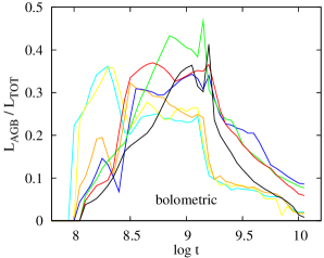
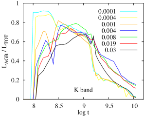
Figure 2: Relative contributions of the TP-AGB phase to the total luminosity of a SSP using the new isochrones. The ratios are plotted as a function of SSP age, with metallicities listed in the legend. Left panel: bolometric ratios. Right panel: $K$-band ratios.

2.1 The AGB phase contribution to the integrated light

Updates in TP-AGB modelling are expected to affect CMLR involving NIR bands, where TP-AGB stars dominate, by up to 80%, the luminosity of SSPs of intermediate ages 0.3–3 Gyr (Figure 2); see Maraston (1998, 2005). This is supported by observations of LMC clusters (Frogel et al., 1990), where AGB stars contribute up to 40% of the bolometric luminosity in said age range.

In Figure 3, we compare the $M_{\star}/L$ evolution of the old and new SSPs in $K$ band. The onset of the AGB phase, soon after 100 Myr, is smoother in the new models: the “AGB phase transition” is not as sharp, due to revised mass–loss prescriptions that reduce the lifetimes of the most massive TP-AGB stars (Marigo et al., 2008). Later on though, the new models remain significantly brighter in the NIR (up to 0.5 mag), predicting “lighter” $M_{\star}/L$ ratios for most of the SSP lifetime. In bluer bands, the difference between old and new models is reduced, becoming negligible in $UBV$.

As a minor detail, notice that the new $Z=0.004$ SSP presents a spike of high $M_{\star}/L_{K}$ (and a corresponding blue spike in $(V-K)$, see Fig. 4) around $\log t=8.4$. As the NIR luminosity is very sensitive to the contribution of carbon stars, this feature can be ascribed to the complex dependence of the carbon star phase as a function of stellar mass and age for this particular metallicity (see Fig. 20 in Marigo & Girardi, 2007). The spike is however smoothed away in the case of composite stellar populations.

For solar and LMC metallicity we also compare to the models of Maraston (2005) — her $Z=0.02$ and 0.01 SSPs respectively: the $M_{\star}/L_{K}$ evolution is qualitatively similar to that of the new Padova models, although the onset of the AGB contribution occurs at $t>200$ Myr. While this difference is relevant for star clusters within that specific age range, it is less crucial for the integrated light and CMLR of galaxies with extended star formation histories, where the two models globally agree (see Fig. 5). A detailed comparison to the Maraston models is beyond the scopes of this paper; some comparison can be found in Marigo et al. (2008) and Conroy et al. (2009); Conroy & Gunn (2010) — though notice that the latter authors adopt different spectral libraries, and tailor their own version of the default Padova models considered here.

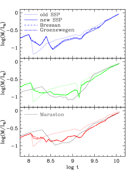
Figure 3: $K$ band $M_{\star}/L$ ratio as a function of age for the “old” (dotted) and “new” (solid) SSPs. The effect of circumstellar dust on the “new” SSPs is also shown (dashed lines). Top panel: $Z$=0.004; Mid panel: $Z$=0.008; bottom panel: $Z=Z_{\odot}$=0.019. Notice that the luminosity peak around $\log t=9.2$, most prominent for $Z=0.008$, is a non–spurious, understood feature of SSPs (Girardi & Bertelli, 1998); it is so short-lived, however, that it is smoothed away when considering composite stellar populations with finite age range. For solar and LMC metallicity (bottom panels) we also overplot the corresponding SSPs from Maraston (2005) rescaled, for the sake of this comparison, from Salpeter to Kroupa (1998) IMF by accountig for the approriate evolutionary flux (Maraston 1998).

2.2 Circumstellar dust

The new Padova isochrones can also include circumstellar dust around AGB stars, following the recipes of Bressan et al. (1998) or Groenewegen (2006). The circumstellar envelope reprocesses a fraction of the stellar UV/optical light to the mid and far infrared. The process is crucial to interpret the MIR HR diagram of the Magellanic Clouds (Marigo et al. 2008, 2010; see also Boyer et al., 2009; Kelson & Holden, 2010; Barmby & Jalilian, 2012) but NIR light is much less affected.

Figure 3 also compares the NIR $M_{\star}/L$ of new SSPs with and without circumstellar dust; the difference is tiny compared to that between the old and the new models. Dust effects on NIR light are highlighted in two–colour plots such as $(J-H)$ vs. $(H-K)$ (Bressan et al., 1998; Piovan et al., 2003), but we verified that, for the sake of CMLR, even for these colours the impact of dust is smaller than the difference between the old and the new SSPs.

In bluer bands the difference between dusty and dust-free SSPs remains negligible, as the optical luminosity of SSPs is not so sensitive to the AGB phase (Maraston, 1998, 2005); so, albeit the optical emission of AGB stars does suffer from dust reprocessing, this is of minor importance for the SSP as a whole.

In short, the impact of circumstellar dust on integrated SSP light is far less crucial than the improved TP-AGB modelling, and we shall neglect it in the remainder of this work.

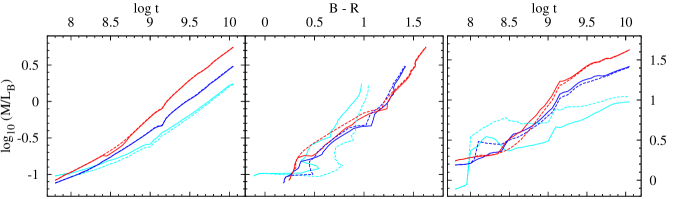
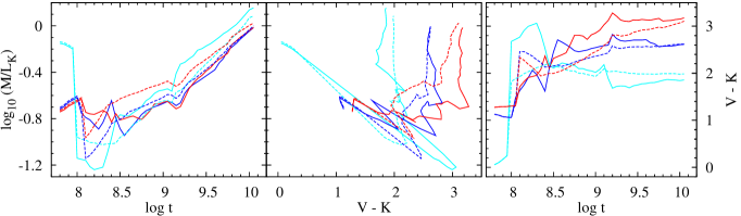
Figure 4: Comparison of SSP evolution and CMLR between the old (dashed) and the new (solid) datasets. Three metallicities are shown: $Z$=0.0001 (cyan), 0.004 (blue) and 0.019 (red).

2.3 Time evolution of colours and mass-to-light

Figure 4 exemplifies the origin of CMLR for SSPs, as the combined result of the time evolution of colours and $M_{\star}/L$. We selected for illustration three metallicities: $Z$=0.0001 is the lowest in the database; $Z$=0.004 and 0.019, corresponding to SMC and solar metallicity, cover the range significant for the bulk of stellar populations in galaxies.

The top panels show a typical optical CMLR: both $M_{\star}/L$ and colour smoothly increase with SSP age and the resulting CMLR does not significantly depend on metallicity, at least in the range $Z=0.004-0.02$. The new implementation of the TP-AGB phase has very mild effects in optical bands: the AGB “phase transition” is not apparent in optical colours, dominated by the light of turn-off Main Sequence stars and core helium–burning stars (Renzini & Buzzoni, 1986; Bressan et al., 1994; Maraston, 1998, 2005). Only at very low metallicities, where young SSPs are much bluer, we see an AGB colour transition.

The bottom panels in Fig. 4 illustrate a typical optical–NIR CMLR, where the difference between old and new models is far more evident. The $(V-K)$ colour tends to saturate, becoming mainly a metallicity indicator, after $t=0.3$ Gyr. Correspondingly, the optical—NIR CMLR for SSPs breaks down at old ages (cf. the almost vertical lines in the middle panel). With the new SSPs, the evolution of the $K$ band $M_{\star}/L$ ratio is very similar for $0.004\leq Z\leq 0.019$; this degeneracy with respect to metallicity was already remarked by Maraston (2005).

Table 2: Grid of $b$ parameter values and corresponding e–folding timescales $\tau$ for our exponential models.

$b$	0.01	0.05	0.10	0.15	0.20	0.30	0.40	0.50	0.60	0.70	0.80	0.90	1.00
	1.10	1.23	1.37	1.55	1.75	2.01	2.35	2.84	3.23	3.67	4.59	6.46	8.33	10.00
$\tau$	1.55	2.20	2.80	3.25	3.80	4.90	6.20	8.00	10.50	15.00	23.00	50.00	$\infty$
	-50.00	-23.00	-15.00	-10.50	-8.00	-6.20	-4.90	-3.80	-3.25	-2.80	-2.20	-1.55	-1.20	-1.00

3 Colour–$M_{\star}/L$ relations for exponential models

Composite stellar populations — convolutions of SSPs of different age and metallicity, according to a given star formation and chemical evolution history — are more relevant for practical applications of CMLR to real galaxies. In this section we shall consider exponentially declining (or increasing) Star Formation Rates (SFR), a common recipe to mimic the photometric properties of the Hubble sequence.

The age of our models is $T=10$ Gyr (the age estimate for the Milky Way disc; Carraro, 2000). For each metallicity, we compute a grid of 27 exponential models with SFR $\Psi(t)\propto e^{-t/\tau}$: declining SFR are modelled with e–folding timescales $\tau$ ranging from 1.55 Gyr to $\infty$ (constant star formation rate); increasing SFR are modelled with negative values of $\tau$ ranging from $-50.00$ to $-1.00$.

These star formation histories (SFHs) can be characterized by the “birthrate parameter” $b=\psi(T)/{\langle\psi\rangle}$: the ratio between present–day and past average SFR. This can be considered a tracer of morphological galaxy type, with $b<0.2$ for Sa–Sab discs, $b\sim 0.4$ for Sb discs and $b\sim 1$ for Sc discs (Kennicutt, Tamblyn & Congdon, 1994; Sommer-Larsen, Götz & Portinari, 2003). Therefore, exponential models with $b\leq 1$ schematically represent “normal” spiral galaxies; models with $b>1$ represent blue galaxies with prominent recent star formation. Elliptical galaxies are typically well represented by old SSPs ($b\longrightarrow 0$).

The range of adopted $\tau$ and $b$ values (from 0.01 to 10.0) are tabulated in Table 2. Our grid of exponential models is similar to that considered by Bell et al. (2003).

Figure 5: Mass-to-light ratio in $I$ and $K$ band for exponential models of different metallicity, as a function of the $b$ parameter. Solid lines represent the new models and dashed lines the old models. The right panels show the full range of model SFH with $b=0.1-10$; the left panels zoom on the more “normal” $b\leq 1$. The black dot–dashed line shows the K–band $M_{\star}/L$ from the Maraston SSPs (Z=0.01).

Figure 6: $K$ band mass-to-light vs. $B-R$ (upper panel) and $V-K$ (lower panel). Solid/dashed lines for new/old models, as in Figure 5. The thick part of the curves marks the case $b\leq 1$, representative of the SFH of “normal” galaxies.

3.1 Effects of updated TP-AGB models

We now compare the CMLR of exponential SFHs, derived from the old and the new SSPs, mostly for $Z\geq 0.004$ as the relevant metallicity range for integrated galaxy light.

In Figure 5 we plot the $M_{\star}/L$ ratio of exponential models versus $b$ parameter. As already shown for SSPs, the optical luminosity is only marginally affected by the update: the new models are brighter just by $\leq$0.03 dex in $I$ band. In NIR bands, the new TP-AGB implementation renders the models brighter up to 0.1 dex (or 25%); the difference is largest at solar metallicity. With the new models, the dependence of $M_{\star}/L_{K}$ on metallicity is largely reduced (Fig. 4 and Maraston 2005): NIR $M_{\star}/L$ ratios depend on the SFH of the system but not much on the underlying chemical enrichment history and metallicity distribution. This is convenient when deriving stellar masses from NIR luminosity; in comparison, for $M_{\star}/L_{I}$ the metallicity dependence is as strong as the SFH dependence (at least for $b\leq 1$).

In Fig. 6 we plot CMLR for $M_{\star}/L_{K}$ versus $(B-R)$ and $(V-K)$ colours, a popular choice for estimating stellar masses (Kranz et al., 2003; Kassin et al., 2006). The effect of the new SSPs on the $M_{\star}/L_{K}-(B-R)$ relation is an overall brightening by 0.1–0.15 dex at any fixed $(B-R)$, as the latter is quite insensitive to TP-AGB modelling (see Fig. 4). This is in general the case for CMLR based on optical colours.

In optical–NIR colours instead, the new models are up to 0.3 mag redder than the old models. As a combined result of brightening and reddening, the $M_{\star}/L_{K}$ ratio at a given colour is up to 0.3 dex, or 2 times, lighter. Factor–of–2 lighter masses were indeed derived by Maraston (2006) from multi-band photometry of galaxies at $z\sim 2$, thanks to the AGB contribution in their models.

Also, the $M_{\star}/L_{K}-(V-K)$ relation depends more strongly on metallicity for the new models, as $(V-K)$ is more of a metallicity tracer than a $M_{\star}/L$ tracer (see Fig. 4). Similar comments hold for other optical–NIR colours.

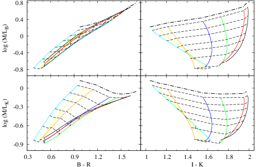
Figure 7: CMLR combining $B$ and $K$ band $M_{\star}/L$ versus $(B-R)$ and $(I-K)$ colours for the full range of $b$ parameters and metallicities. The solid lines connect models with the same metallicity (colour coding as in Fig. 2); the dashed lines connect models with the same $b$ parameter: from top to bottom, $b=$ 0.01, 0.15, 0.40, 1.00, 1.75, 3.67, 10.00. The dash-dotted line represents a pure SSP of age 10 Gyr.

In Figure 7 we show the new CMLR for $B$ and $K$ band $M_{\star}/L$ versus $(B-R)$ and $(I-K)$, for all the metallicities (coloured solid lines) and a representative sampling of the $b$–parameter range 0.01–10 (dashed lines). The CMLR for a 10 Gyr old SSP is added as a dot–dashed line, smoothly extending the CMLR of the exponential models with the lowest $b$ values.

We confirm the tight correlation between $B$ band $M_{\star}/L$ ratio and the optical $(B-R)$ colour, very little affected by SFH and metallicity — other than possibly for the lowest $Z=0.0001$ case. Such a degree of age and metallicity degeneracy ensures robust CMLR in the optical.

CMLR remain quite robust even for $K$ band $M_{\star}/L$ versus $(B-R)$: the age–metallicity degeneracy is quite tight for $Z\geq 0.004$, breaking down only for lower metallicities that are seldom relevant in integrated galaxy light.

In $(I-K)$, the age–metallicity degeneracy breaks down (Bell & de Jong, 2001) for this is mainly a metallicity indicator, like $(V-K)$. (For the lowest metallicities, the dependence of $(I-K)$ on $Z$ gets “inverted” for $b>1$ — i.e. when the system is dominated by young stellar populations. We ascribe this behaviour to the fact that the extended C star phase of the more massive AGB stars causes a greater colour transition toward the red, the lower the metallicity; see Fig. 20 in Marigo & Girardi 2007). CMLR in $(I-K)$ are not very meaningful. The same holds for redder (purely NIR, e.g. $J-K$) colours and for $(V-K)$; while $(B-K)$ yields reasonably tight CMLR for $Z\geq 0.008$, the LMC metallicity.

We provide in Table 3 log–linear CMLR for exponential models, for those colours that reasonably trace the $M_{\star}/L$ ratio, at least in the metallicity range relevant for galaxies ($Z\geq 0.004$). These CMLR fit the detailed model results within $\pm$0.1 dex (25% accuracy in $M_{\star}/L$); asterisks indicate less tight CMLR, accurate within $\pm$0.13 dex (35% error).

As a rule, the fits are based on models with $0.004\leq Z\leq 0.03$, but for optical–optical colours the same fits are good also down to much lower metallicities. In few cases, meaningful fits are limited to $Z\geq 0.008$. The metallicity range where the fit is valid is indicated in the table.

Among optical colours, $(R-I)$ and $(r-i)$ are the least reliable $M_{\star}/L$ indicators; their use is further discouraged by their short baseline, as the error on the colour will have a significant impact on the practical estimate of $M_{\star}/L$ (see also Gallazzi & Bell, 2009).

In Table 3 we also provide CMLR for SDSS colours; they are steeper — lighter at the blue end — than those of Bell et al. (2003). This is partly due to the fact that their semi–empirical relations are intrinsically flatter than the theoretical ones (BdJ or PST04), partly due to the fact that our new models result in somewhat steeper CMLR even for optical colours (see Section 4).

Table 3: Fitting coefficients of CMLR of the form : $\log(M_{\star}/L)=s\times{\rm colour}+z$ from exponential SFH models with Kroupa IMF; the colour range covered by the models is indicated at the bottom of each sub-table. The rightmost column indicates the metallicity range $Z\geq Z_{min}$ where the fitted CMLR apply (see text). Asterisks indicate less tight CMLR (accuracy of $\pm$0.13 dex rather than $\pm$0.1 dex).

colour	$\log(M_{\star}/L)$	$s$	$z$	$Z_{min}$
$(B-V)$	$B$	1.866	-1.075	0.0004
$(B-V)$	$V$	1.466	-0.807	0.0004
$(B-V)$	$R$	1.277	-0.720	0.0004
$(B-V)$	$I$	1.147	-0.704	0.0004
$(B-V)$	$J$	1.047	-0.850	0.004
$(B-V)$	$H$	1.030	-0.992	0.004
$(B-V)$	$K$	1.064	-1.066	0.004
$(B-V)$	$J^{2M}$	1.031	-0.835	0.004
$(B-V)$	$H^{2M}$	1.024	-0.991	0.004
$(B-V)$	$Ks^{2M}$	1.055	-1.066	0.004
0.2–1.0
$(B-R)$	$B$	1.272	-1.287	0.0004
$(B-R)$	$V$	1.000	-0.975	0.0004
$(B-R)$	$R$	0.872	-0.866	0.0004
$(B-R)$	$I$	0.783	-0.836	0.001
$(B-R)$	$J$	0.714	-0.969	0.004
$(B-R)$	$H$	0.701	-1.109	0.004
$(B-R)$	$K$	0.724	-1.186	0.004
$(B-R)$	$J^{2M}$	0.702	-0.952	0.004
$(B-R)$	$H^{2M}$	0.697	-1.107	0.004
$(B-R)$	$Ks^{2M}$	0.718	-1.185	0.004
0.5–1.6
$(B-I)$	$B$	1.041	-1.549	0.001
$(B-I)$	$V$	0.819	-1.182	0.001
$(B-I)$	$R$	0.714	-1.047	0.001
$(B-I)$	$I$	0.641	-0.997	0.004
$(B-I)$	$J$	0.582	-1.112	0.004
$(B-I)$	$H$	0.571	-1.249	0.004
$(B-I)$	$K$	0.589	-1.330	0.004
$(B-I)$	$J^{2M}$	0.572	-1.094	0.004
$(B-I)$	$H^{2M}$	0.567	-1.245	0.004
$(B-I)$	$Ks^{2M}$	0.583	-1.327	0.004
0.7–2.2
$(B-K)$	$B$	0.898	-3.009	0.008
$(B-K)$	$V$	0.710	-2.335	0.008
$(B-K)$	$R$	0.620	-2.054	0.008
$(B-K)$	$I$	0.556	-1.901	0.008
$(B-K)$*	$J$	0.498	-1.927	0.008
$(B-K)$*	$H$	0.487	-2.047	0.008
$(B-K)$*	$K$	0.498	-2.141	0.008
2.6–4.2
$(B-Ks)$	$B$	0.894	-3.047	0.008
$(B-Ks)$	$V$	0.707	-2.367	0.008
$(B-Ks)$	$R$	0.618	-2.082	0.008
$(B-Ks)$	$I$	0.555	-1.928	0.008
$(B-Ks)$*	$J^{2M}$	0.489	-1.922	0.008
$(B-Ks)$*	$H^{2M}$	0.484	-2.069	0.008
$(B-Ks)$*	$Ks^{2M}$	0.494	-2.166	0.008
2.6–4.2
$(V-R)$	$B$	3.963	-1.728	0.004
$(V-R)$	$V$	3.124	-1.325	0.004
$(V-R)$	$R$	2.724	-1.172	0.004
$(V-R)$	$I$	2.443	-1.109	0.004
$(V-R)$	$J$	2.220	-1.215	0.004
$(V-R)$	$H$	2.178	-1.349	0.004
$(V-R)$	$K$	2.248	-1.434	0.004
$(V-R)$	$J^{2M}$	2.186	-1.195	0.004
$(V-R)$	$H^{2M}$	2.166	-1.346	0.004
$(V-R)$	$Ks^{2M}$	2.228	-1.431	0.004
0.25–0.65

colour	$\log(M_{\star}/L)$	$s$	$z$	$Z_{min}$
$(V-I)$	$B$	2.312	-2.111	0.004
$(V-I)$	$V$	1.826	-1.629	0.004
$(V-I)$	$R$	1.593	-1.438	0.004
$(V-I)$	$I$	1.426	-1.346	0.004
$(V-I)$	$J$	1.285	-1.420	0.004
$(V-I)$*	$H$	1.257	-1.547	0.004
$(V-I)$*	$K$	1.296	-1.637	0.004
$(V-I)$	$J^{2M}$	1.265	-1.397	0.004
$(V-I)$*	$H^{2M}$	1.249	-1.541	0.004
$(V-I)$*	$Ks^{2M}$	1.282	-1.630	0.004
0.6–1.2
$(R-I)$*	$B$	5.436	-2.594	0.004
$(R-I)$*	$V$	4.304	-2.016	0.004
$(R-I)$*	$R$	3.756	-1.776	0.004
$(R-I)$*	$I$	3.357	-1.645	0.004
$(R-I)$*	$J$	2.955	-1.674	0.008
$(R-I)$*	$H$	2.898	-1.804	0.008
$(R-I)$*	$K$	2.965	-1.891	0.008
$(R-I)$*	$J^{2M}$	2.934	-1.661	0.008
$(R-I)$*	$H^{2M}$	2.907	-1.813	0.008
$(R-I)$*	$Ks^{2M}$	2.975	-1.906	0.008
0.35–0.60
$(g-r)$	$g$	1.774	-0.783	0.0004
$(g-r)$	$r$	1.373	-0.596	0.0004
$(g-r)$	$i$	1.227	-0.576	0.001
$(g-r)$	$z$	1.158	-0.619	0.001
$(g-r)$	$J^{2M}$	1.068	-0.728	0.004
$(g-r)$	$H^{2M}$	1.060	-0.884	0.004
$(g-r)$	$Ks^{2M}$	1.091	-0.956	0.004
0.1–0.85
$(g-i)$	$g$	1.297	-0.855	0.001
$(g-i)$	$r$	1.005	-0.652	0.001
$(g-i)$	$i$	0.897	-0.625	0.001
$(g-i)$	$z$	0.845	-0.665	0.004
$(g-i)$	$J^{2M}$	0.779	-0.769	0.004
$(g-i)$	$H^{2M}$	0.772	-0.924	0.004
$(g-i)$	$Ks^{2M}$	0.794	-0.997	0.004
0.1–1.2
$(g-z)$	$g$	1.152	-0.991	0.004
$(g-z)$	$r$	0.896	-0.759	0.004
$(g-z)$	$i$	0.800	-0.721	0.004
$(g-z)$	$z$	0.752	-0.754	0.004
$(g-z)$	$J^{2M}$	0.683	-0.844	0.004
$(g-z)$*	$H^{2M}$	0.673	-0.995	0.004
$(g-z)$*	$Ks^{2M}$	0.691	-1.069	0.004
0.3–1.5
$(r-i)$*	$g$	4.707	-1.025	0.004
$(r-i)$*	$r$	3.650	-0.784	0.004
$(r-i)$*	$i$	3.251	-0.741	0.004
$(r-i)$*	$z$	3.054	-0.773	0.004
$(r-i)$*	$J^{2M}$	2.806	-0.867	0.004
$(r-i)$*	$H^{2M}$	2.768	-1.018	0.004
$(r-i)$*	$Ks^{2M}$	2.843	-1.093	0.004
0.07–0.34
$(r-z)$	$g$	3.101	-1.323	0.008
$(r-z)$	$r$	2.395	-1.007	0.008
$(r-z)$	$i$	2.128	-0.937	0.008
$(r-z)$	$z$	1.995	-0.958	0.008
$(r-z)$	$J^{2M}$	1.864	-1.067	0.008
$(r-z)$	$H^{2M}$	1.843	-1.223	0.008
$(r-z)$	$Ks^{2M}$	1.885	-1.302	0.008
0.2–0.62

3.2 Comparison to old literature and to the no–TPAGB case

To highlight the importance of the TP-AGB phase for CMLR, we compare to the previous theoretical relations of Bell & de Jong (2001, hereafter BdJ), based on an early release of the GALAXEV population synthesis package by Bruzual & Charlot (2003). Our Fig. 8 mimics Fig. 2 of BdJ by limiting to exponentially decreasing SFHs ($b\leq 1$, representative of “normal” galaxies) and mostly plotting the same metallicities (albeit their plot extends up to $Z=0.05$ and ours down to $Z=0.0001$). The two figures are directly comparable, safe for a systematic offset in $M_{\star}/L$ zero-point of about 0.2 dex, due to the different IMF (Salpeter vs. Kroupa) and older age (12 vs. 10 Gyr) in their models.

The bottom panel of Fig. 8 excludes the contribution of the TP-AGB phase (we computed no–TPAGB SSPs from the Padova isochrones, halting integration at the mass point where the Mhec flag marks the extension to the TP-AGB phase). The outcome is remarkably similar to Fig. 2 of BdJ, reasserting that early versions of GALAXEV effectively neglected the TP-AGB contribution (Maraston, 2005), although this has improved in later versions (Bruzual, 2007).

With respect to the no–TPAGB case, the optical CMLR becomes marginally less tight in the range $Z=0.004-0.03$, while $(I-K)$ becomes an even more neat metallicity indicator, independent of SFH. Most interesting is the $M_{\star}/L_{K}$–$(B-R)$ CMLR: the “wedge” pattern in the no–TPAGB case, also seen in BdJ, significantly changes when the TP-AGB phase is included: this CMLR becomes lighter, steeper, and tighter in the metallicity range $Z=0.004-0.03$. The same applies to NIR $M_{\star}/L$ versus optical colours in general.

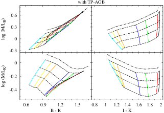
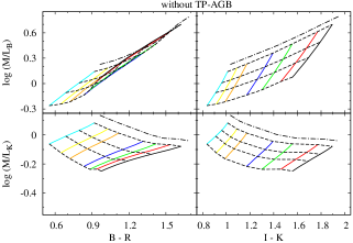
Figure 8: Same as Fig. 7, but limited to $b\leq 1$. In the lower panel, the TP-AGB phase has been excluded.

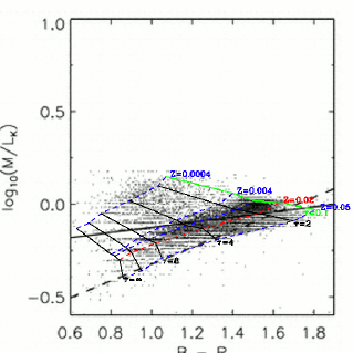
Figure 9: Reproduction of Fig. 20 by Bell et al. (2003): location of galaxies with multi-band SDSS+2MASS photometry in the $M/L_{K}$ vs. $(B-R)$ plane; the solid line is the “semi–empirical” CMLR derived by Bell et al. the dashed line is the theoretical relation of BdJ. Overlayed is a grid of exponential models obtained by BdJ with population synthesis models available at the time.

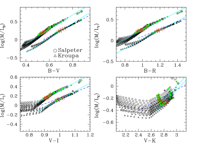
Figure 10: CMLR for the chemo–photometric models of disc galaxies of PST04 with Salpeter and Kroupa IMF, updated with the new SSP set. Symbols as in Fig. B1 of PST04. Open symbols: one–zone models for individual disc annuli; filled symbols: multi–zone models (integrated photometry of bulge region, disc region, or global galaxy); asterisks, “optical disc” region; see PST04 for more details. The solid lines represent the linear fits for the different IMFs; the dashed line is the superseded CMLR of PST04 for the Kroupa IMF.

The “wedge” pattern in the $M_{\star}/L_{K}$–$(B-R)$ relation, typical of population synthesis models of the early 2000’s, directly reflected in the multi–band analysis of the galaxy mass function of Bell et al. (2003). In Fig. 9 we reproduce their Fig. 20, where each galaxy was assigned a location in the CMLR plane by $\chi^{2}$–optimization within the underlying grid of exponential SFH models; to this we overlay the theoretical grid from Fig. 2 of BdJ, vertically shifted to adjust it to the IMF normalization adopted by Bell et al. Clearly the colour–$M_{\star}/L$ pattern predicted at the time beared on the estimated $M_{\star}/L$ ratios and on the resulting “semi–empirical” CMLR of Bell et al. (2003), that is much flatter than the original theoretical relation of BdJ and has been widely used thereafter. Considering the rather different CMLR predicted by modern models, and the crucial role of NIR light in determining stellar mass, those results on the stellar mass function and semi–empirical CMLR are worth a revision.

Also, we argue against the blind application of semi-empirical relations established for the galaxy population as a whole, when interpreting photometric properties within individual galaxies (e.g. Kassin et al., 2006). The very flat slope of the semi–empirical CMLR of Bell et al. (2003) is evidently driven by a population of objects with very blue optical colours but high NIR $M_{\star}/L$ ratios, that stands aside of the rest of the trend as very metal–poor (dwarf?) galaxies with old stellar populations. Their chemical and photometric properties are then quite different from those found within normal disc galaxies, so that CMLR derived including these objects do not apply to colour profiles in spiral galaxies.

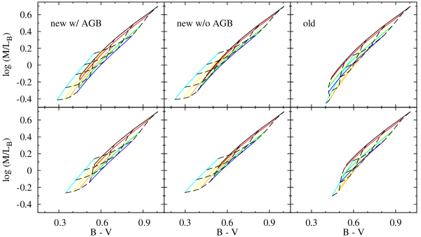
Figure 11: CMLR for $M_{\star}/L_{B}$ vs. $(B-V)$ for the exponential models with $b\leq 2$ (top panels) or $b\leq 1$ (bottom panels). Left: CMLR from the “new” SSP dataset; middle: excluding the contribution of the TP-AGB phase; right: CMLR from the “old” dataset.

4 Colour–$M_{\star}/L$ relations for disc galaxy models

In this section we recompute the CMLR for the disc galaxy models of Portinari et al. (2004, hereinafter PST04) and discuss the updated CMLR relevant within individual galaxies.

Fig. 10 reproduces Fig. B1 of PST04 with the new photometric models — showing only the Salpeter and Kroupa IMF case for clarity. The old CMLR of PST04 for the Kroupa IMF case are shown as dashed lines for comparison. For purely optical CMLR (top panels) the new and old CMLR differ at the blue end: the old CMLR were linear down to a certain break point in colour (the blue limit of the dashed lines; see also Fig. B1 in PST04), below which $M_{\star}/L$ quickly dropped. In the new CMLR, the relation steepens toward the blue (say, below 0.6 in $B-V$, 0.9 in $B-R$) with no abrupt break; this smoother trend reflects that of the new SSPs in Fig. 4 (top mid panel). Still, a single linear fit is adequate over a wide colour range, with a slope somewhat steeper than in the CMLR of PST04. The fitting coefficients are listed in Table 4 and Table 5. (Notice that disc models cover a smaller colour range than the exponential models, as SFHs and metallicities do not get as extreme as considered in the previous section.)

The break/steepening of the optical CMLR at the blue end seems supported by observations (McGaugh, 2005) so it is worth commenting in detail. In the inside–out scenario, disc galaxies are characterized by radial gradients in metallicity and SFH: blue colours in the disc outskirts result from a combination of low metallicities and slow SFHs ($b\simeq 1$). To illustrate the consequence of this folding, Fig. 11 displays the $M_{\star}/L_{B}-(B-V)$ relation from exponential models. For SFHs typical of “normal” galaxies ($b\leq 1$, bottom panels) around $(B-V)=0.5$ there’s a shift from $Z\geq 0.004$ to $Z<0.004$: bluer colours can only be obtained for lower metallicities, which for a given SFH (e.g., $b=1$) have systematically lower optical $M_{\star}/L$. Indeed, the old CMLR of PST04 had a break in $M_{\star}/L$ at $(B-V)\simeq 0.5$. The effect is stronger when the TP-AGB phase is properly included (left panels vs. mid panels) and was even stronger with the old TP-AGB prescriptions of Girardi & Bertelli (1998) (right panels), that led to the abrupt break in the CMLR of PST04 — while no such effect was seen in the BdJ models for global galaxies. This shows that, albeit linear $\log M_{\star}/L$—colour relations are a reasonable and handy approximation over a very large range in colours, for detailed studies it is worth to consider realistic chemical evolution models and the role of the mass–metallicity relation (for galaxies in general) or of metallicity gradients (within individual objects).

As the drop in $M_{\star}/L$ at the blue end is favoured by the data (McGaugh, 2005), it would be interesting to apply the new, smoother but steeper CMLR. In any case, in the outskirts of disc galaxies the $M_{\star}/L$ ratio should be lower than predicted by the BdJ recipe (and by the even flatter semi–empirical relations of Bell et al., 2003).

When considering red or NIR bands (bottom panels in Fig. 10), the CMLR relation flattens out at the blue end, with a large scatter. This is also consequence of the metallicity gradients: blue colours correspond to the metal–poor outskirts of discs, and at low $Z$ red–NIR $M_{\star}/L$ ratios tend to be larger and do not follow tight CMLR (Fig. 8, left panels). In Table 4 and 5 we indicate the blue limit for the log–linear CMLR, below which flattening occurs and scatter in $M_{\star}/L$ at given colour becomes significant, exceeding $\pm 0.1$ dex.

The bottom right panel of Fig. 10 shows $M_{\star}/L_{K}$ vs. $(V-K)$, representative of optical–NIR CMLR in general. As $(V-K)$ is mostly a metallicity tracer, rather than a $M_{\star}/L$ tracer, the new relation is very steep at the red end (central regions of disc galaxies with high metallicities) and flattens out below $(V-K)=2.6$, presenting everywhere a large scatter. Though we still provide CMLR based on optical–NIR colours in Table 4, we remark with asterisks that these colours are not good tracers of $M_{\star}/L$.

Optical colours should always be preferred — even when estimating NIR $M_{\star}/L$ (Fig. 12). The new optical colour—NIR $M_{\star}/L$ relations are steeper, with lower $M_{\star}/L$ at a given colour; and are nicely tight down to some blue limit ($\sim$0.9 for $B-R$) below which they display the typical flattening and large scatter of the low metallicity regimes.

We remark again that, when studying the profiles of disc galaxies (for the sake of decomposing rotation curves, for instance) this sort of steep CMLR should be adopted, as they correspond to self–consistent folding of SF and metal enrichment histories, with low metallicities always associated to slow SFH and young stellar populations in the outer regions. “Global” CMLR for the galaxy population as a whole (Bell et al., 2003) are much flatter due to the contribution of galaxies with metal–poor old populations (Fig. 9), that have no counterpart in disc galaxies. Depending on the type of problem at hand, the suitable set of CMLR (“local” or “global”, theoretical or semi–empirical) should be adopted.

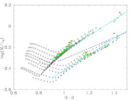
Figure 12: $M_{\star}/L_{K}$ vs. $(B-R)$ relation for the disc galaxy models of PST04. Lines and symbols as in Fig. 10.

Table 4: Fitting coefficients of CMLR of the form : $\log(M_{\star}/L)=s\times{\rm colour}+z$ from disc galaxy models. Zero–points are given for the Kroupa and the Salpeter IMF normalizations. Asterisks warn against those colours that are not optimal $M_{\star}/L$ tracers. For NIR $M_{\star}/L$ ratios, we also indicate the blue limit below which the relation flattens out (see text). The colour range effectively covered by the disc galaxy models is indicated at the bottom of each sub-table.

colour	$M_{\star}/L$	$s$	$z_{Kr}$	$z_{Salp}$	blue lim
$(B-V)$	$B$	2.027	-1.168	-0.933
$(B-V)$	$V$	1.627	-0.900	-0.665
$(B-V)$	$R$	1.438	-0.811	-0.580
$(B-V)$	$I$	1.294	-0.782	-0.559
$(B-V)$	$J$	1.074	-0.832	-0.634	$>$0.5
$(B-V)$	$H$	1.042	-0.958	-0.770	$>$0.5
$(B-V)$	$K$	1.070	-1.023	-0.836	$>$0.5
$(B-V)$	$J^{2M}$	1.050	-0.812	-0.618	$>$0.5
$(B-V)$	$H^{2M}$	1.032	-0.953	-0.767	$>$0.5
$(B-V)$	$Ks^{2M}$	1.054	-1.020	-0.837	$>$0.5
0.35–0.9
$(B-R)$	$B$	1.374	-1.384	-1.164
$(B-R)$	$V$	1.106	-1.077	-0.855
$(B-R)$	$R$	0.974	-0.964	-0.744
$(B-R)$	$I$	0.870	-0.912	-0.699
$(B-R)$	$J$	0.753	-0.976	-0.785	$>$0.9
$(B-R)$	$H$	0.731	-1.098	-0.916	$>$0.9
$(B-R)$	$K$	0.750	-1.168	-0.987	$>$0.9
$(B-R)$	$J^{2M}$	0.735	-0.953	-0.765	$>$0.9
$(B-R)$	$H^{2M}$	0.723	-1.093	-0.913	$>$0.9
$(B-R)$	$Ks^{2M}$	0.739	-1.162	-0.985	$>$0.9
0.7–1.45
$(B-I)$	$B$	1.141	-1.688	-1.480	$>$1.25
$(B-I)$	$V$	0.916	-1.317	-1.103	$>$1.25
$(B-I)$	$R$	0.814	-1.187	-0.974	$>$1.25
$(B-I)$	$I$	0.741	-1.136	-0.928	$>$1.25
$(B-I)$	$J$	0.638	-1.166	-0.977	$>$1.40
$(B-I)$	$H$	0.627	-1.297	-1.115	$>$1.40
$(B-I)$	$K$	0.641	-1.367	-1.187	$>$1.40
$(B-I)$	$J^{2M}$	0.627	-1.145	-0.958	$>$1.40
$(B-I)$	$H^{2M}$	0.625	-1.297	-1.116	$>$1.40
$(B-I)$	$Ks^{2M}$	0.638	-1.370	-1.192	$>$1.40
1.0–2.0
$(B-K)$	$B$	0.892	-2.860	-2.741	$>$3.0
$(B-K)$	$V$	0.719	-2.269	-2.125	$>$3.0
$(B-K)$	$R$	0.643	-2.046	-1.895	$>$3.0
$(B-K)$	$I$	0.592	-1.942	-1.789	$>$3.0
$(B-K)$*	$J$	0.508	-1.855	-1.721	$>$3.1
$(B-K)$*	$H$	0.495	-1.960	-1.833	$>$3.1
$(B-K)$*	$K$	0.504	-2.037	-1.914	$>$3.1
2.4–3.9
$(B-Ks)$	$B$	0.903	-2.950	-2.831	$>$3.1
$(B-Ks)$	$V$	0.724	-2.330	-2.185	$>$3.1
$(B-Ks)$	$R$	0.646	-2.096	-1.944	$>$3.1
$(B-Ks)$	$I$	0.595	-1.988	-1.834	$>$3.1
$(B-Ks)$*	$J^{2M}$	0.509	-1.886	-1.754	$>$3.2
$(B-Ks)$*	$H^{2M}$	0.507	-1.034	-0.908	$>$3.2
$(B-Ks)$*	$Ks^{2M}$	0.516	-2.116	-1.995	$>$3.2
2.5–3.9
$(V-R)$	$B$	4.321	-1.867	-1.682	$>$0.38
$(V-R)$	$V$	3.478	-1.465	-1.270	$>$0.38
$(V-R)$	$R$	3.078	-1.313	-1.118	$>$0.38
$(V-R)$	$I$	2.773	-1.235	-1.044	$>$0.38
$(V-R)$	$J$	2.430	-1.270	-1.101	$>$0.40
$(V-R)$	$H$	2.311	-1.359	-1.201	$>$0.40
$(V-R)$	$K$	2.386	-1.442	-1.285	$>$0.40
$(V-R)$	$J^{2M}$	2.353	-1.230	-1.064	$>$0.40
$(V-R)$	$H^{2M}$	2.267	-1.341	-1.185	$>$0.40
$(V-R)$	$Ks^{2M}$	2.315	-1.415	-1.263	$>$0.40
0.32–0.58
$(V-I)$	$B$	2.677	-2.423	-2.253	$>$0.85
$(V-I)$	$V$	2.156	-1.916	-1.732	$>$0.85
$(V-I)$	$R$	1.922	-1.724	-1.538	$>$0.85
$(V-I)$	$I$	1.756	-1.632	-1.448	$>$0.85
$(V-I)$	$J$	1.549	-1.629	-1.464	$>$0.88
$(V-I)$	$H$	1.508	-1.738	-1.580	$>$0.88
$(V-I)$	$K$	1.546	-1.822	-1.667	$>$0.88
$(V-I)$	$J^{2M}$	1.513	-1.592	-1.429	$>$0.88
$(V-I)$	$H^{2M}$	1.495	-1.729	-1.573	$>$0.88
$(V-I)$	$Ks^{2M}$	1.528	-1.812	-1.659	$>$0.88
0.70–1.14

colour	$M_{\star}/L$	$s$	$z_{Kr}$	$z_{Salp}$	blue lim
$(V-J)$*	$B$	1.648	-2.924	-2.862	$>$1.7
$(V-J)$*	$V$	1.348	-2.358	-2.259	$>$1.7
$(V-J)$*	$R$	1.213	-2.141	-2.030	$>$1.7
$(V-J)$*	$I$	1.126	-2.047	-1.930	$>$1.7
$(V-J)$*	$J$	0.992	-1.991	-1.890	$>$1.8
$(V-J)$*	$H$	0.985	-2.127	-2.031	$>$1.8
$(V-J)$*	$K$	1.009	-2.220	-2.128	$>$1.8
1.35–2.15
$(V-J^{2M})$*	$B$	1.478	-2.669	-2.611	$>$1.75
$(V-J^{2M})$*	$V$	1.197	-2.126	-2.031	$>$1.75
$(V-J^{2M})$*	$R$	1.072	-1.923	-1.815	$>$1.75
$(V-J^{2M})$*	$I$	0.988	-1.832	-1.718	$>$1.75
$(V-J^{2M})$*	$J^{2M}$	0.947	-1.951	-1.850	$>$1.85
$(V-J^{2M})$*	$H^{2M}$	0.959	-2.129	-2.033	$>$1.85
$(V-J^{2M})$*	$Ks^{2M}$	0.982	-2.226	-2.135	$>$1.85
1.4–2.2
$(V-H)$*	$B$	1.610	-4.011	-3.969	$>$2.45
$(V-H)$*	$V$	1.336	-3.297	-3.214	$>$2.45
$(V-H)$*	$R$	1.180	-2.927	-2.830	$>$2.45
$(V-H)$*	$I$	1.094	-2.773	-2.670	$>$2.45
$(V-H)$*	$J$	0.981	-2.679	-2.589	$>$2.50
$(V-H)$*	$H$	0.979	-2.823	-2.738	$>$2.50
$(V-H)$*	$K$	1.000	-2.925	-2.844	$>$2.50
1.9–2.9
$(V-H^{2M})$*	$B$	1.571	-3.956	-3.917	$>$2.45
$(V-H^{2M})$*	$V$	1.282	-3.194	-3.114	$>$2.45
$(V-H^{2M})$*	$R$	1.153	-2.892	-2.797	$>$2.45
$(V-H^{2M})$*	$I$	1.070	-2.744	-2.643	$>$2.45
$(V-H^{2M})$*	$J^{2M}$	0.941	-2.599	-2.512	$>$2.50
$(V-H^{2M})$*	$H^{2M}$	0.954	-2.789	-2.707	$>$2.50
$(V-H^{2M})$*	$Ks^{2M}$	0.976	-2.899	-2.822	$>$2.50
1.95–2.90
$(V-K)$*	$B$	1.689	-4.465	-4.443	$>$2.60
$(V-K)$*	$V$	1.373	-3.595	-3.528	$>$2.60
$(V-K)$*	$R$	1.231	-3.242	-3.159	$>$2.60
$(V-K)$*	$I$	1.141	-3.064	-2.973	$>$2.60
$(V-K)$*	$J$	1.034	-2.970	-2.892	$>$2.65
$(V-K)$*	$H$	1.035	-3.123	-3.050	$>$2.65
$(V-K)$*	$K$	1.054	-3.222	-3.153	$>$2.65
2.05–3.00
$(V-Ks^{2M})$*	$B$	1.628	-4.382	-4.363	$>$2.65
$(V-Ks^{2M})$*	$V$	1.331	-3.549	-3.485	$>$2.65
$(V-Ks^{2M})$*	$R$	1.198	-3.214	-3.134	$>$2.65
$(V-Ks^{2M})$*	$I$	1.113	-3.046	-2.958	$>$2.65
$(V-Ks^{2M})$*	$J^{2M}$	0.979	-2.867	-2.791	$>$2.72
$(V-Ks^{2M})$*	$H^{2M}$	0.991	-3.056	-2.985	$>$2.72
$(V-Ks^{2M})$*	$Ks^{2M}$	1.015	-3.176	-3.110	$>$2.72
2.1–3.1
$(R-I)$	$B$	7.003	-3.315	-3.172	$>$0.45
$(R-I)$	$V$	5.614	-2.620	-2.457	$>$0.45
$(R-I)$	$R$	5.005	-2.354	-2.186	$>$0.45
$(R-I)$	$I$	4.605	-2.223	-2.054	$>$0.45
$(R-I)$	$J$	3.964	-2.099	-1.955	$>$0.47
$(R-I)$	$H$	3.862	-2.196	-2.059	$>$0.47
$(R-I)$	$K$	3.955	-2.290	-2.156	$>$0.47
$(R-I)$	$J^{2M}$	3.874	-2.052	-1.910	$>$0.47
$(R-I)$	$H^{2M}$	3.834	-2.186	-2.050	$>$0.47
$(R-I)$	$Ks^{2M}$	3.915	-2.278	-2.146	$>$0.47
0.37–0.57

Table 5: Same as Table 4 but for SDSS colours.

colour	$\log(M_{\star}/L)$	$s$	$z_{Kr}$	$z_{Salp}$	blue lim
$(g-r)$	$g$	1.930	-0.851	-0.634
$(g-r)$	$r$	1.530	-0.663	-0.445
$(g-r)$	$i$	1.370	-0.633	-0.420
$(g-r)$	$z$	1.292	-0.665	-0.462	$>$0.3
$(g-r)$	$J^{2M}$	1.139	-0.732	-0.544	$>$0.4
$(g-r)$	$H^{2M}$	1.128	-0.880	-0.699	$>$0.4
$(g-r)$	$Ks^{2M}$	1.153	-0.945	-0.767	$>$0.4
0.25–0.75
$(g-i)$	$g$	1.385	-0.899	-0.698	$>$0.5
$(g-i)$	$r$	1.098	-0.702	-0.498	$>$0.5
$(g-i)$	$i$	0.985	-0.669	-0.468	$>$0.5
$(g-i)$	$z$	0.898	-0.675	-0.484	$>$0.5
$(g-i)$	$J^{2M}$	0.868	-0.804	-0.621	$>$0.6
$(g-i)$	$H^{2M}$	0.861	-0.952	-0.776	$>$0.6
$(g-i)$	$Ks^{2M}$	0.879	-1.019	-0.847	$>$0.6
0.35–1.05
$(g-z)$	$g$	1.294	-1.097	-0.908	$>$0.7
$(g-z)$	$r$	1.033	-0.867	-0.669	$>$0.7
$(g-z)$	$i$	0.946	-0.838	-0.642	$>$0.7
$(g-z)$	$z$	0.894	-0.861	-0.672	$>$0.7
$(g-z)$	$J^{2M}$	0.789	-0.906	-0.734	$>$0.8
$(g-z)$	$H^{2M}$	0.787	-1.060	-0.893	$>$0.8
$(g-z)$	$Ks^{2M}$	0.803	-1.128	-0.965	$>$0.8
0.7–1.3
$(r-i)$	$g$	5.926	-1.293	-1.116	$>$0.20
$(r-i)$	$r$	4.738	-1.025	-0.838	$>$0.20
$(r-i)$	$i$	4.338	-0.982	-0.795	$>$0.20
$(r-i)$	$z$	4.093	-0.996	-0.816	$>$0.20
$(r-i)$	$J^{2M}$	3.684	-1.043	-0.878	$>$0.21
$(r-i)$	$H^{2M}$	3.659	-1.192	-1.033	$>$0.21
$(r-i)$	$Ks^{2M}$	3.740	-1.264	-1.109	$>$0.21
0.12–0.32
$(r-z)$	$g$	3.902	-1.592	-1.466	$>$0.38
$(r-z)$	$r$	3.116	-1.263	-1.116	$>$0.38
$(r-z)$	$i$	2.863	-1.205	-1.054	$>$0.38
$(r-z)$	$z$	2.716	-1.214	-1.067	$>$0.38
$(r-z)$	$J^{2M}$	2.355	-1.196	-1.067	$>$0.40
$(r-z)$	$H^{2M}$	2.344	-1.346	-1.223	$>$0.40
$(r-z)$	$Ks^{2M}$	2.384	-1.416	-1.297	$>$0.40
0.22–0.56

5 Attenuation by interstellar dust

We have discussed in Section 2.2 that circumstellar dust around AGB stars has a negligible effect on optical and NIR CMLR, so that we can disregard it. In this section we address the effect of interstellar dust, that both reddens and dims stellar luminosity. Bell & de Jong (2001) argue that, to first order, in optical CMLR the two effects compensate each other, as the dust vector runs almost parallel to the dust–free CMLR (age–metallicity–dust degeneracy).

We revisit the effects of interstellar dust on optical and NIR CMLR over galactic scales, taking advantage of recent recipes based on detailed radiative transfer models (Tuffs et al., 2004). Our goal is to provide CMLR that are statistically applicable to large galaxy samples that include a range of morphologies, intrinsic colours and random inclinations.

5.1 The attenuated spiral galaxy models

We construct simple models of spiral galaxies consisting of bulge+disc, and then apply the dust corrections of Tuffs et al. (2004). The models include a bulge component, represented by a 10 Gyr old SSP, and a disc component with exponential SFH with $b\leq 2$ (Section 3): $b\leq 1$ values represent “normal” disc galaxy morphologies, and we extend to somewhat bluer objects with recent intensive SF. For simplicity, the dust–free models were calculated only for solar metallicity: we shall see that dust effects on galactic scales are statistically more relevant than metallicity effects.

The models have a random distribution in $b=0.01\div 2$ and in bulge–to–total ratio B/T=$0\div 0.6$, typical of disc galaxies (Allen et al., 2006); the corresponding luminosity ratios (B/T)_λ entering Eq. 1 below, are computed self–consistently from the SFHs for bulge and disc. Dust attenuation is then added for random inclinations from face-on to edge–on, $0\leq\cos(i)\leq 1$, for a total of 20000 models.

Dust attenuation in the various bands is computed following the prescriptions of Tuffs et al. (2004), to which the reader is referred for all details. Their dust models have been successfully tested both on multi–band emission of individual galaxies (Popescu et al., 2000) and on large galaxy surveys (Driver et al., 2007). The attenuation prescriptions of Tuffs et al. depend only on the properties of interstellar dust, not on the incident stellar radiation field, and are presented as applicable to real disc galaxies irrespectively of their detailed stellar SED; likewise, they are applicable to model disc galaxies irrespectively of the specific population synthesis model used to generate them.

Figure 13: CMLR for dust–free model galaxies (black dots) and attenuated models (red dots). The solid line indicates the linear fit to the attenuated models.

In short, the dust model includes a clumpy dust component associated with the star-forming regions in a thin disc (which affects only UV light, and can be neglected in the optical/NIR; Popescu et al., 2000; Tuffs et al., 2004) and a diffuse dust component residing both in the young thin disc and in the older disc. The bulge is intrinsically dust–free, but is heavily affected by the dust in the disc, to the extent that it turns out to be the most attenuated galaxy component; a counter–intuitive result confirmed by observational trends (Driver et al., 2007). The equation for the composite attenuation of the galaxy at wavelength $\lambda$ is:

$$\Delta m_{\lambda}=-2.5\log\Bigg{(}r^{\mathrm{0,disc}}_{\lambda}10^{-0.4\Delta m^{\mathrm{disc}}_{\lambda}}+r^{\mathrm{0,bulge}}_{\lambda}10^{-0.4\Delta m^{\mathrm{bulge}}_{\lambda}}\Bigg{)}$$ (1)

where $r^{0}_{\lambda}$ is the fraction of the bulge or disc to the total intrinsic luminosity in the band $\lambda$: (B/T)_λ and (1-B/T)_λ, respectively. (We recast the equation in terms of the intrinsic B/T ratio of the galaxy models, while the original Eq. 18 in Tuffs et al. was expressed in terms of the apparent, dust–attenuated B/T ratio, to be applied to observed galaxies.) $\Delta m^{\mathrm{disc,bulge}}_{\lambda}$ is the attenuation value in magnitudes for the disc or bulge, provided by Tuffs et al. in the form of polynomial equations in $(1-\cos i)$. The polynomial coefficients are tabulated for various optical and NIR photometric bands, and optical depth values $\tau_{B}^{f}$. We use the fixed value $\tau^{f}_{B}=4.0$, consistent with the empirical mean opacity $\tau_{B}^{f}=3.8\,\pm\,0.7$ found by Driver et al. (2007) based on 10095 galaxies with bulge-disc decomposition.

We notice in passing that Eq. 1 becomes inconsistent for high B/T values, as it predicts an ever–increasing attenuation for increasing bulge fraction, while in the limit B/T $\longrightarrow$ 1 attenuation should vanish together with the disc component. We suspect that this is a consequence of extending the disc+dust to the very centre, rather than modelling a hole in the dusty disc in correspondence to the bulge component. However, here we only consider galaxies with an important disc component (B/T $\leq$ 0.6) where the dust prescriptions of Tuffs et al. are well supported by observational evidence (Driver et al., 2007).

5.2 Colour–$M_{\star}/L$ relations for dusty galaxies

Fig. 13 shows the effects of dust on various CMLR. The dust–free galaxies (black dots) are intrinsically redder with decreasing disc $b$–parameter and increasing B/T ratio. They follow, within the quoted uncertainty of 0.1 dex, the CMLR predicted by the exponential models of Section 3: the superposition of two components, disc+bulge (exponential SFH + old SSP) still closely follow the one–component CMLR — but there is hardly any CMLR in $(I-K)$, as discussed in Section 3. When dust attenuation is taken into account (red dots), the models spread on a much wider area in the plot, the brighter (fainter) bound corresponding to face–on (edge–on) inclinations.

The top panels show optical CMLR. The spread in $\log M_{\star}/L$ at a fixed colour is about 0.5 dex (a factor–of–3), with dusty galaxies being tipically less luminous than the dust–free case. Notice that the red end of the dust–free distribution is scattered much further to the red by attenuation, than the blue end; this is another counter–intuitive result of the bulge component suffering more extinction than the disc. The largest departures from the dust–free case correspond to the highest inclinations, that are statistically less frequent; altogether the statistical CMLR of attenuated galaxies (solid line) is not too far from the dust–free exponential case of Section 3. In the $\log M_{\star}/L$ vs. $(B-R)$ plane the dusty CMLR is mildly offset (0.1 dex) from the dust–free one, toward heavier $M_{\star}/L_{B}$ at fixed colour.

The (statistical) effect of dust is smallest for $M_{\star}/L_{V}$ vs. $(V-I)$: the attenuated CMLR just shows a bit steeper slope than the dust–free one, and the difference is even less than 0.1 dex. This is interesting as Gallazzi & Bell (2009) have recently selected $(g-i)$ as the best suited colour for stellar mass estimates in the dust–free case. As this colour is quite close to $(V-I)$, we argue that dust corrections are small for CMLR involving $(g-i)$, so that this is a robust optical $M_{\star}/L$ indicator also with respect to dust effects. (We cannot address the role of dust attenuation directly in SDSS bands, as the Tuffs et al. prescriptions are only provided for Johnson bands.)

Table 6: Fitting coefficients of CMLR of the form : $\log(M_{\star}/L)=s\times{\rm colour}+z$ for dusty galaxy models.

colour	$\log(M_{\star}/L)$	$s$	$z$
$(B-V)$	$B$	1.836	-0.905
$(B-V)$	$V$	1.493	-0.681
$(B-V)$	$R$	1.337	-0.627
$(B-V)$	$I$	1.228	-0.646
$(B-V)$	$J$	1.048	-0.803
$(B-V)$	$H$	0.941	-0.909
$(B-V)$	$K$	0.866	-0.926
0.5–1.1
$(B-R)$	$B$	1.272	-1.173
$(B-R)$	$V$	1.040	-0.905
$(B-R)$	$R$	0.934	-0.832
$(B-R)$	$I$	0.860	-0.837
$(B-R)$	$J$	0.730	-0.960
$(B-R)$	$H$	0.652	-1.047
$(B-R)$	$K$	0.599	-1.051
0.9–1.8
$(B-I)$	$B$	1.049	-1.492
$(B-I)$	$V$	0.859	-1.167
$(B-I)$	$R$	0.772	-1.069
$(B-I)$	$I$	0.711	-1.057
$(B-I)$	$J$	0.602	-1.142
$(B-I)$	$H$	0.537	-1.209
$(B-I)$	$K$	0.493	-1.200
1.4–2.5
$(B-J)$	$B$	0.886	-2.203
$(B-J)$	$V$	0.724	-1.746
$(B-J)$	$R$	0.649	-1.585
$(B-J)$	$I$	0.597	-1.527
$(B-J)$	$J$	0.505	-1.541
$(B-J)$	$H$	0.452	-1.567
$(B-J)$	$K$	0.416	-1.532
2.4–3.9
$(B-H)$	$B$	0.803	-2.604
$(B-H)$	$V$	0.656	-2.073
$(B-H)$	$R$	0.588	-1.876
$(B-H)$	$I$	0.540	-1.793
$(B-H)$	$J$	0.457	-1.767
$(B-H)$	$H$	0.409	-1.771
$(B-H)$	$K$	0.377	-1.720
3.2–4.8
$(B-K)$	$B$	0.734	-2.496
$(B-K)$	$V$	0.600	-1.984
$(B-K)$	$R$	0.537	-1.797
$(B-K)$	$I$	0.493	-1.719
$(B-K)$	$J$	0.418	-1.705
$(B-K)$	$H$	0.374	-1.716
$(B-K)$	$K$	0.345	-1.670
3.4–5.2

colour	$\log(M_{\star}/L)$	$s$	$z$
$(V-R)$	$B$	3.966	-1.697
$(V-R)$	$V$	3.308	-1.356
$(V-R)$	$R$	2.953	-1.227
$(V-R)$	$I$	2.700	-1.191
$(V-R)$	$J$	2.301	-1.266
$(V-R)$	$H$	2.071	-1.328
$(V-R)$	$K$	1.911	-1.314
0.4–0.7
$(V-I)$	$B$	2.404	-2.223
$(V-I)$	$V$	1.959	-1.756
$(V-I)$	$R$	1.752	-1.589
$(V-I)$	$I$	1.606	-1.526
$(V-I)$	$J$	1.365	-1.547
$(V-I)$	$H$	1.225	-1.577
$(V-I)$	$K$	1.129	-1.542
0.9–1.4
$(V-J)$	$B$	1.587	-3.129
$(V-J)$	$V$	1.296	-2.501
$(V-J)$	$R$	1.161	-2.259
$(V-J)$	$I$	1.066	-2.143
$(V-J)$	$J$	0.902	-2.065
$(V-J)$	$H$	0.808	-2.038
$(V-J)$	$K$	0.744	-1.966
1.9–2.7
$(V-H)$	$B$	1.266	-3.428
$(V-H)$	$V$	1.034	-2.746
$(V-H)$	$R$	0.927	-2.479
$(V-H)$	$I$	0.851	-2.345
$(V-H)$	$J$	0.729	-2.235
$(V-H)$	$H$	0.645	-2.191
$(V-H)$	$K$	0.595	-2.110
2.7–3.8
$(V-K)$	$B$	1.048	-2.979
$(V-K)$	$V$	0.856	-2.379
$(V-K)$	$R$	0.767	-2.150
$(V-K)$	$I$	0.704	-2.044
$(V-K)$	$J$	0.597	-1.981
$(V-K)$	$H$	0.535	-1.966
$(V-K)$	$K$	0.414	-1.640
2.9–4.2
$(I-K)$	$B$	0.970	-1.632
$(I-K)$	$V$	0.885	-1.480
$(I-K)$	$R$	0.831	-1.428
$(I-K)$	$I$	0.786	-1.430
$(I-K)$	$J$	0.627	-1.376
$(I-K)$	$H$	0.505	-1.298
$(I-K)$	$K$	0.386	-1.114
2.0–2.7

The role of dust is remarkable in optical–NIR CMLR (bottom panels): inclination strongly influences the colours, and the strong reddening renders the dusty optical–NIR CMLR lighter, at a given colour, than the dust–free case.

Since the dust–free optical–NIR CMLR depend on metallicity, we checked that changing the metallicity of the galaxy models (within a factor of 2–3 from solar, as relevant for global galaxy metallicities) has very little impact on the resulting dusty CMLR: the effect of dust is dominant over metallicity effects.

In some optical–NIR CMLR, attenuation and reddening combine so as to maintain tight CMLR — albeit different from the dust–free case. The best example is $(B-K)$, with a $M_{\star}/L$ scatter of at most $\pm$0.15 dex in all bands (bottom left panel). Also $(V-H)$ is a good $M_{\star}/L$ tracer for dusty galaxies, with a scatter of $\pm$0.15 dex in $M_{\star}/L_{V}$ or $M_{\star}/L_{H}$ at given $(V-H)$. Even for the $(I-K)-M_{\star}/L_{I}$ relation, the scatter ($\pm$0.2 dex) is no worse than that for optical dusty CMLR (bottom right).

In summary, when dust attenuated galaxies are considered, optical–NIR CMLR are no worse (in terms of scatter) than optical–optical CMLR; in some cases — notably $(B-K)$ — they are even favoured. The best option in dusty optical–NIR CMLR is to derive $M_{\star}/L$ in one of the bands involved in the base colour; a very common case in practice.

6 Summary and conclusions

In this paper we rediscuss theoretical colour–stellar mass-to-light relations (CMLR) in the light of modern populations synthesis models including an accurate implementation of the TP-AGB phase, and of the effects of interstellar dust as predicted from radiative transfer models of disc galaxies.

The importance of the AGB phase for the integrated NIR luminosity of stellar populations has been extensively discussed in recent years (Maraston, 2005, 2006; Tonini et al., 2009, and other papers of the same series). In intermediate–age stellar populations (0.3–2 Gyr), TP-AGB stars dominate the NIR luminosity, lowering the $M_{\star}/L$ ratio by up to a factor of 2 and driving very red optical–NIR colours ($V-K\geq 3$); NIR $M_{\star}/L$ ratios are quite independent of metallicity. Optical luminosities and colours, on the other hand, are not severely affected.

We update theoretical CMLR for composite stellar populations by means of the latest Padova isochrones (Marigo et al. 2008; Girardi et  al. 2010), which include a far more refined treatment of the TP-AGB phase than the previous dataset (Girardi & Bertelli, 1998; Girardi et al., 2002).

For most of their evolution after the onset of the AGB at $\sim$100 Myr, the updated Single Stellar Populations are significanly brighter in the NIR (up to 0.5 mag), with correspondingly “lighter” $M_{\star}/L$. The effect of circumstellar dust on the integrated optical and NIR luminosity is negligible.

Considering both Simple and composite Stellar Populations (the latter with exponentially decreasing/increasing star formation histories mimicking the Hubble sequence, as well as from full chemo–photometric galaxy models) we highlight the following characteristics of updated CMLR.

• Optical CMLR are little affected by the upgrade in the AGB models, and remain tight thanks to a strong age–metallicity degeneracy (cf. Bell & de Jong, 2001).

• The integrated NIR luminosity is increased with minor effects in the optical: the resulting NIR $M_{\star}/L$ is about 0.1 dex lighter, at a given optical colour.

• The integrated NIR luminosity is also less sensitive to metallicity — at least for $Z\geq 0.004$ which is representative of the bulk of the stellar populations in galaxies. This favours a more robust estimate of stellar mass from NIR light, with tighter NIR $M_{\star}/L$—optical colour relations (like $M_{\star}/L_{K}$ vs. $B-R$) compared to previous predictions.

• In optical–NIR colours, such as $(V-K)$, the new models are both lighter and redder, so that the new CMLR are much lighter (up to 0.3 dex, a factor of 2) at a given colour.

• As noticed by Bell & de Jong (2001), optical–NIR colours like $(V-K)$ or $(I-K)$ are mostly metallicity indicators, while being very poor $M_{\star}/L$ tracers; this is even more true with the new models.

• The new models suggests a revision of results obtained from multi–band analysis of the galaxy population spanning from optical to NIR, including semi–empirical CMLR (Bell et al., 2003).

• We argue against the use of semi–empirical CMLR established for the general galaxy population, when studying individual galaxies: the CMLR resulting from a coherent star formation and chemical evolution history (and their radial gradients) within a single galaxy is potentially different from the CMLR obtained as a statistical average of galaxies. This is evident for instance in the “break” of the CMLR at blue optical colours, seen in chemo–photometric models of disc galaxies (Portinari et al., 2004) and not when considering a wider range of (uncorrelated) SFH and metallicities describing the galaxy population in general.

We finally warn that recent observational results suggest that the newest population synthesis models may actually overestimate the luminosity contribution of AGB stars (Kriek et al. 2010; Zibetti et al., 2012), partly due to an excess of rare, luminous AGB stars in the models (Melbourne et al. 2010) and partly due to the effects of circumstellar dust (Meidt et al. 2012) . Future, better calibrated AGB models may converge on CMLR intermediate between the “classic” ones of the early 2000’s and those presented here.

All of the above refers to dust–free CMLR. It is usually assumed that, at least for optical CMLR, dust is a second–order effect thanks to the age–metallicity–dust degeneracy (Bell & de Jong, 2001). We revisited this issue considering a more realistic implementation of dust effects on galactic scales, and found that dust has a non–negligible role.

• The combined effect of reddening and attenuation introduces an enormous scatter even in optical CMLR: highly inclined disc galaxies can be 0.5 dex “heavier” at a given colour, than predicted by dust–free CMLR. So, for individual galaxies, the CMLR does not apply unless good inclination information and dust corrections are available.

• Nontheless, we can still define “dusty” CMLR that statistically apply to large galaxy samples where we lack detailed morphological and inclination information for individual objects (but are at least able to distinguish a disc–like galaxy from a pure spheroid with no dust). In the optical, statistical dusty CMLR are somewhat heavier (about 0.1 dex) at a given colour, than the dust-free case.

• The smallest change with respect to the dust–free case is found for $M_{\star}/L_{V}$ vs. $(V-I)$. This suggests that the $(g-i)$ colour, recently selected as optimal stellar mass tracer in the dust–free case (Gallazzi & Bell, 2009), remains a good tracer also when considering (or neglecting!) the effects of dust.

• Dust reddening strongly alters optical–NIR CMLR, making them lighter, at given colour, than dust–free CMLR.

• For some optical–NIR CMLR, extinction and reddening combine to yield rather tight dusty CMLR — albeit very different from the dust–free ones. $(B-K)$ is an excellent stellar mass tracer for dusty galaxies, with a scatter in $M_{\star}/L$ within $\pm$0.15 dex in all bands. $M_{\star}/L_{V,H}$ vs. $(V-H)$ CMLR are also similarly tight. For dusty galaxies, these CMLR are better mass tracers than optical–optical CMLR.

In Tables 3 through 6 we give our updated CMLR for the various cases: exponential models (for those colours where defining a CMLR is meaningful, at least for $Z\geq 0.004$); chemo–photometric disc galaxy models, where CMLR result from a consistent convolution of SF and chemical evolution history, to be best applied within individual (dust–free or dust–corrected) galaxies; and “dusty” CMLR that can be statistically applied to large galaxy samples.

CMLR are a robust, handy tool to estimate stellar masses; we can optimize their use by choosing the colour and relation most suitable for each specific problem.

References

- Allen et al. (2006) Allen P. D., Driver S. P., Graham A. W., Cameron E., Liske J., Propris R. D., 2006, Mon. Not. R. Astron. Soc., 371, 2
- Bakos et al. (2008) Bakos J., Trujillo I., Pohlen M., 2008, Astrophys. J., Lett., 683, 103
- Barmby & Jalilian (2012) Barmby P., Jalilian F. F., 2012, Astron. J., 143, 87
- Bell & de Jong (2001) Bell E. F., de Jong R. S., 2001, Astrophys. J., 550, 212
- Bell & et al. (2004) Bell E. F., et al. 2004, Astrophys. J., 608, 752
- Bell et al. (2003) Bell E. F., McIntosh D. H., Katz N., Weinberg M. D., 2003, Astrophys. J., Suppl. Ser., 149, 289
- Boissier & Prantzos (1999) Boissier S., Prantzos N., 1999, Mon. Not. R. Astron. Soc., 307, 857
- Boyer et al. (2009) Boyer M. L., Skillman E. D., van Loon J. T., Gehrz R. D., Woodward C. E., 2009, Astrophys. J., 697, 1993
- Bressan et al. (1994) Bressan A., Chiosi C., Fagotto F., 1994, Astrophys. J., Suppl. Ser., 94, 63
- Bressan et al. (1998) Bressan A., Granato G. L., Silva L., 1998, Astron. Astrophys., 332, 135
- Bruzual (2007) Bruzual G., 2007, in Vallenari A., Tantalo R., Portinari L., Moretti A., eds, From Stars to Galaxies: Building the Pieces to Build Up the Universe Vol. 374 of ASP Conf.Ser., Stellar populations: High spectral resolution libraries. improved tp-agb treatment. Publ. Astron. Soc. Pac., San Francisco, p. 303
- Bruzual & Charlot (2003) Bruzual G., Charlot S., 2003, Mon. Not. R. Astron. Soc., 344, 1000
- Carraro (2000) Carraro G., 2000, in F. Matteucci & F. Giovannelli ed., The Evolution of the Milky Way: Stars versus Clusters The Age of the Galactic Disk. pp 335–346
- Chabrier (2001) Chabrier G., 2001, Astrophys. J., 554, 1274
- Chabrier (2002) Chabrier G., 2002, Astrophys. J., 567, 304
- Conroy & Gunn (2010) Conroy C., Gunn J. E., 2010, Astrophys. J., 712, 833
- Conroy et al. (2009) Conroy C., Gunn J. E., White M., 2009, Astrophys. J., 699, 486
- Driver et al. (2007) Driver S. P., Popescu C. C., Tuffs R. J., Liske J., Graham A. W., Allen P. D., Propris R. D., 2007, Mon. Not. R. Astron. Soc., 379, 1022
- Flynn et al. (2006) Flynn C., Holmberg J., Portinari L., Fuchs B., Jahreiß H., 2006, Mon. Not. R. Astron. Soc., 372, 1149
- Frogel et al. (1990) Frogel J. A., Mould J., Blanco V. M., 1990, Astrophys. J., 352, 96
- Fukugita et al. (1998) Fukugita M., Hogan C. J., Peebles P. J. E., 1998, Astrophys. J., 503
- Fukugita & Peebles (2004) Fukugita M., Peebles P. J. E., 2004, Astrophys. J., 616, 643
- Gallazzi & Bell (2009) Gallazzi A., Bell E. F., 2009, Astrophys. J., Suppl. Ser., 185, 253
- Girardi & Bertelli (1998) Girardi L., Bertelli G., 1998, Mon. Not. R. Astron. Soc., 300, 533
- Girardi et al. (2002) Girardi L., Bertelli G., Bressan A., Chiosi C., Groenewegen M. A. T., Marigo P., Salasnich B., Weiss A., 2002, Astron. Astrophys., 391, 195
- Girardi et al. (2000) Girardi L., Bressan A., Bertelli G., Chiosi C., 2000, Astron. Astrophys. Suppl. Ser., 141, 371
- Girardi & et al. (2010) Girardi L., et al. 2010, Astrophys. J., 724, 1030
- Groenewegen (2006) Groenewegen M. A. T., 2006, Astron. Astrophys., 448, 181
- Jablonka & Arimoto (1992) Jablonka J., Arimoto N., 1992, Astron. Astrophys., 255, 63
- Kassin et al. (2006) Kassin S. A., de Jong R. S., Weiner B. J., 2006, Astrophys. J., 643, 804
- Kelson & Holden (2010) Kelson D. D., Holden B. P., 2010, Astrophys. J., Lett., 713, L28
- Kennicutt et al. (1994) Kennicutt R. C. J., Tamblyn P., Congdon C. W., 1994, Astrophys. J., 435, 22
- Kranz et al. (2003) Kranz T., Slyz A., Rix H.-W., 2003, Astrophys. J., 586, 143
- Kriek & et al. (2010) Kriek M., et al. 2010, Astrophys. J., Lett., 722, L64
- Kroupa (1998) Kroupa P., 1998, in Rebolo R., Martin E., Zapatero Osorio M., eds, Brown Dwarfs and Extrasolar Planets Vol. 134 of ASP Conf.Ser., The stellar mass function. Publ. Astron. Soc. Pac., San Francisco, p. 483
- Kroupa (2001) Kroupa P., 2001, Mon. Not. R. Astron. Soc., 322, 231
- Larson & Tinsley (1978) Larson R. B., Tinsley B. M., 1978, Astrophys. J., 219, 46
- Maraston (1998) Maraston C., 1998, Mon. Not. R. Astron. Soc., 300, 872
- Maraston (2005) Maraston C., 2005, Mon. Not. R. Astron. Soc., 362, 799
- Maraston (2006) Maraston C., 2006, Astrophys. J., 652, 85
- Marigo & et al. (2010) Marigo M., et al. 2010, in Bruzual G., Charlot S., eds, IAU Symposium Vol. 262 of IAU Symposium, TP-AGB stars in population synthesis models. pp 36–43
- Marigo (2001) Marigo P., 2001, Astron. Astrophys., 370, 194
- Marigo & Girardi (2007) Marigo P., Girardi L., 2007, Astron. Astrophys., 469, 239
- Marigo et al. (2008) Marigo P., Girardi L., Bressan A., Groenewegen M. A. T., Silva L., Granato G. L., 2008, Astron. Astrophys., 482, 883
- McGaugh (2004) McGaugh S. S., 2004, Astrophys. J., 609, 652
- McGaugh (2005) McGaugh S. S., 2005, Astrophys. J., 632, 859
- McGaugh et al. (2010) McGaugh S. S., Schombert J. M., de Blok W. J. G., Zagursky M. J., 2010, Astrophys. J., Lett., 708, L14
- Meidt & et al. (2012) Meidt S., et al. 2012, Astrophys. J., Lett., 748, L30
- Melbourne & et al. (2012) Melbourne J., et al. 2012, Astrophys. J., 748, 47
- Mouhcine & Lançon (2002) Mouhcine M., Lançon A., 2002, Astron. Astrophys., 393, 149
- Mouhcine & Lançon (2003) Mouhcine M., Lançon A., 2003, Astron. Astrophys., 402, 425
- Persic et al. (1993) Persic M., Salucci P., Ashman K. M., 1993, Astron. Astrophys., 279, 343
- Piovan et al. (2003) Piovan L., Tantalo R., Chiosi C., 2003, Astron. Astrophys., 408, 559
- Piovan et al. (2006) Piovan L., Tantalo R., Chiosi C., 2006, Mon. Not. R. Astron. Soc., 370, 1454
- Popescu et al. (2000) Popescu C. C., Misiriotis A., Kylafis N. D., Tuffs R. J., Fischera J., 2000, Astron. Astrophys., 362, 138
- Portinari et al. (1998) Portinari L., Chiosi C., Bressan A., 1998, Astron. Astrophys., 334, 505
- Portinari & Salucci (2010) Portinari L., Salucci P., 2010, Astron. Astrophys., 521, A82+
- Portinari et al. (2004) Portinari L., Sommer-Larsen J., Tantalo R., 2004, Mon. Not. R. Astron. Soc., 347, 691
- Renzini & Buzzoni (1986) Renzini A., Buzzoni A., 1986, in Chiosi C., Renzini A., eds, Spectral Evolution of Galaxies Global properties of stellar populations and the spectral evolution of galaxies. Reidel, Dordrecht, pp 195–235
- Sargent & Tinsley (1974) Sargent W. L. W., Tinsley B. M., 1974, Mon. Not. R. Astron. Soc., 168, 19P
- Silva et al. (1998) Silva L., Granato G. L., Bressan A., Danese L., 1998, Astrophys. J., 509, 103
- Sommer-Larsen et al. (2003) Sommer-Larsen J., Götz M., Portinari L., 2003, Astrophys. J., 596, 47
- Tinsley (1981) Tinsley B. M., 1981, Mon. Not. R. Astron. Soc., 194, 63
- Tonini et al. (2009) Tonini C., Maraston C., Devriendt J., Thomas D., Silk J., 2009, Mon. Not. R. Astron. Soc., 396, L36
- Torres-Flores et al. (2011) Torres-Flores S., Epinat B., Amram P., Plana H., Mendes de Oliveira C., 2011, Mon. Not. R. Astron. Soc., 416, 1936
- Treuthardt et al. (2009) Treuthardt P., Salo H., Buta R., 2009, Astron. J., 137, 19
- Tuffs et al. (2004) Tuffs R. J., Popescu C. C., Völk H., Kylafis N. D., Dopita M., 2004, Astron. Astrophys., 419, 821
- Zibetti et al. (2012) Zibetti S., Gallazzi A., Charlot S., Pierini D., Pasquali A., 2012, MNRAS in press (arXiv:1205.4717)