4cm2.25cm2.2cm2.2cm
Trust in foreseeing neighbours - a novel threshold model of financial market
Abstract
The three-state agent-based 2D model of financial markets in the version proposed by Giulia Iori in 2002 has been herein extended. We have introduced the increase of herding behaviour by modelling the altering trust of an agent in his nearest neighbours. The trust increases if the neighbour has foreseen the price change correctly and the trust decreases in the opposite case. Our version only slightly increases the number of parameters present in the Iori model. This version well reproduces the main stylized facts observed on financial markets. That is, it reproduces log-returns clustering, fat-tail log-returns distribution and power-law decay in time of the volatility autocorrelation function.
PACS numbers: 89.65.Gh, 02.50.Ey, 89.75.Fb, 45.70.Vn.
1 Introduction
The modern study of financial markets has discovered a huge number of phenomena violating the Brownian stochastic dynamics of financial markets. Three major stylized facts observed in the market are exceptionally intriguing: volatility clustering, fat-tail log-return distribution and power-law decay in time of the volatility autocorrelation function. The promising approach to reproduce these phenomena runs through heteroagent-based models where decisions of individual agents somehow determine the price dynamics. Various versions of such models were thoroughly discussed in literature [1-7]. Our version well describes the above mentioned stylized facts by introducing a characteristic emotion to the Iori model. That is, the trust in the foreseeing market agents.
2 Outline of the Iori model
The Giulia Iori model [1] consists of spins or agents placed in 2D square lattice sites, assuming one of the following values of spin states: either as buy, as sell or as stay passive. Each agent, , is under the influence of a local field which is the sum of the forces exerted by the nearest neighbours and by random noise.
Thresholds play a significant role in the Iori model. Thanks to these thresholds, the temporal spin is defined as follows:
| (1) |
where is a time-dependent positive threshold considered below and is a time-dependent local field:
| (2) |
here is a time-dependent force exerted by agent on his neighbouring agent and is a time-dependent white noise describing the agent’s emotion. This force is defined in Section 3.1.
The threshold reflects the symmetry between the probability of buying and selling. The initial threshold is randomly drawn from the Gaussian distribution . Next, it is adjusted in successive time steps after each decision round, according to the rule:
| (3) |
where is a market price of a share at time . For the negative time (i.e. for history before the begining of the simulation) the price values are drawn from a uniform distribution.
In Equation (3) it was tacitly assumed: (i) the proportionality of the threshold to the transaction cost and (ii) proportionality of this transaction cost to the share prices. Iori proved that if the threshold is either zero or constant in time, the stylized facts cannot be properly reproduced.
It is assumed that agents mutually exchange information in a consultation round and they have the opportunity to change their opinion (or spin state) once on average. Hence, the local field can alter. The consultation round is the analogy to the onr Monte Carlo step per spin in Monte Carlo simulations of magnetism. The agents begin trading only after the field is relaxed. It is empirically proven within the Iori model that then the most of spins become constant, which is an analogy to thermalisation of magnetisation in physics.
Subsequently, one calculates the total supply (the total number of negative spins) and demand (the total number of positive spins). Thus, the market maker can determine the current market price according to the following rule:
| (4) |
where market activity
| (5) |
is a slowly-varying function of time and coefficient was assumed as a sufficiently small calibration parameter. Equation (4) describes an asymmetric reaction of the market maker to imbalance between supply and demand. The intensity of this reaction (measured by the value of log-return) depends linearly on the market activity . Equation (4) is consistent with observed positive correlation between absolute log-returns and trading volume (defined, as usual, by quantity related to ). The relation between demand, supply and the price change is differently considered in various agent-based models [6] (and refs. therein). However, the models have to be consistent with the classic economic law of demand and supply.
As usual, the log-return over a time period is defined as a natural logarithm of ratio of the corresponding prices and :
| (6) |
In fact, mainly this definition is exploited in our paper.
3 Our extension: trust in the foreseeing neighbours
3.1 Definition of the impact
The aim of our extension is to define a more realistic impact of a given agent on his neighbours than in the Iori model. This impact is large if the agent has recommended to buy the asset before a price increase or to sell before a price decrease. That is, the impact is large if the product of the spin value at a certain time in the past and the log-return from that time until now is positive. Otherwise, the impact is small. Hence, the force exerted by an agent on his neighbour is:
| (7) |
Coefficient is the value of the initial force allotted at the beginning of the simulation to the pair of investors . It is either with a fixed probability or with complementary probability (as in Iori model) and is the background static influence of agent on agent , randomly drawn from a uniform distribution. The sum over represents the dynamic part of the impact containing a kind of -step memory.
To avoid a persistent positive feedback effect (which results in directed constant price changes), a fundamental behaviour of agents is introduced. This fundamental behaviour is constrained by the fundamental price and two positive factors and . If the market price is greater than the fundamental price multiply by , an agent sells shares. Reversely, if the market price is lower by factor , an agent buys shares.
3.2 Algorithm
Our algorithm makes possible to simulate the behaviour of agents. Single agent can trade only one share at a time that is, he can buy shares only if he possesses enough cash or sell shares only if he has at least one share. Leverage and short sale is beyond the scope of our model.
The algorithm consists of the initial and proper parts. Within the initial part the input values of variables and required parameters are prepared. This part is valid for the case and , where For each value of (at fixed value of ) it consists of the following steps.
-
1.
The spin state, (), of each agent is drawn from a (discrete) 3-point uniform distribution.
-
2.
The price is drawn from unit interval, , by using a uniform continuous distribution.
-
3.
The fixed values (valid for any time) are drawn from interval by using a uniform distribution.
- 4.
-
5.
The intial values of the thresholds are drawn from the normal distribution .
-
6.
The initial values of the -correlated noise, , are drawn from the normal distribution .
-
7.
Cash and shares are granted as well to every agent as to market maker (for details see Section 3.3).
Notably, each time step is divided into two rounds: the consultation and decision ones. In the consultation round only the relaxation of spins occur without changing any amount of cash and shares (of each agent and market maker). The change of cash and shares takes place only in the decision round. This is described in details below.
Within the proper part, valid for , the dynamics of the system is simulated. In this part the dynamics of every agent is determined by the following algorithm.
-
1.
For the spin state of each agent is calculated according to Equation (1), as we have already all quantities required (i.e. those for ). Thus, for all decisions of agents are known.
-
2.
Next, agent is drawn with probability .
-
3.
By using the spin values of ’s nearest neighbours, we construct forces exerted on agent (from his nearest neighbours s) according to Equation (7). This is possible as all required quantities have been calculated one step earlier.
-
4.
Hence, the local field is calculated according to Equation (2).
-
5.
The agent’s threshold is calculated from Equation (3) as all required quantities have been calculated one step earlier.
-
6.
Finally, the spin state is calculated according to Equation (1).
-
7.
The steps 2-6 are repeated until the spin relaxes. This means that decisions of agents stabilise and the consultation round is finished. This relaxation is, in fact, observed in our simulation quite well.
-
8.
The final spin values are the final decisions of all agents. That is, these spin values are the output of the consultation round preceding the decision round in which agents are trading.
-
9.
According to their final decisions (taken at the end of the consultation round), agents put sell or buy orders (being only allowed to trade one share at a given time step) however, the final share prices still have to be defined.
-
10.
The market maker determines the price according to Equation 4.
-
11.
The agents trade, as long as they possess enough shares or cash.
-
12.
Agents who have no sufficient amount of cash or shares, are not able to trade with other agents. Instead, they can trade with the market maker (at prices established in above item) if he has sufficient amount of cash and shares. However, if market maker has no sufficient cash and shares the algorithm stops the current decision round and goes to the subsequent time step.
-
13.
In a given decision round (the number of decision round always equals the number of time steps) the agents demonstrate a fundamental behaviour with probability under the following conditions:
-
•
remainder from dividing the time step (or number) () by a natural number is lower than a fixed value (or , where means the entire part of ). Number is a natural number fixed at the beginning of the simulation, while is also a natural number but drawn from a uniform distribution. As fluctuates, it protects the agent trading against periodicity (which could be present in the case of fixed ). Apparently, for remainder is always smaller than (as it vanishes);
-
•
the market price of share is either higher than the fundamental price multiplied by factor (then the agent can sell a share for the market price) or lower than the fundamental price by factor (then the agent can buy a share for the market price). Indeed, this is a fundamental behaviour of agent because he is driven by the relation between the market price and the fundamental one and not by the collective impact of his neighbours.
-
•
3.3 Comments concerning simulations
The values of parameters of the model have a substantial influence on the accuracy of the reconstruction of stylized facts. For instance, decreasing coefficient (present in Equation (5)) by one order of magnitude (here from to ), increasing the number of agents (here from to ), and decreasing probability of trading according to the fundamental price (here from to ), one gets less accurate results: less visible log-returns clustering and less accurate log-returns distribution.
We performed our simulations, named simulation A and simulation B, which vary only by values of some parameters. The parameter values of simulation A are as follows:
-
•
the number of agents ;
-
•
at the beginning of the simulation each agent a’priori received 100 cash units and the same number of shares. Similarly, the market maker received 10240 cash and shares;
-
•
decision rounds were set and the system’s memory was extended until decision rounds;
-
•
the agents demonstrated a fundamental behaviour (see Algorithm in Section 3.2 for details) if the remainder of dividing the number of decision round by (where and discrete variable was drawn from domain by a uniform distribution) was lower than ; thus they sell shares if their price is times greater than the fundamental price and buy shares if their price is times lower than their fundamental price - both with probability ;
-
•
in every decision round the fundamental value of shares rise by factor ;
-
•
the coefficient from Equation (4) equals .
The values of parameters driving simulation B were assumed the same as in simulation A, except the following ones:
-
•
the system’s memory decision rounds;
-
•
the agents demostrated fundamental behaviour (see Algorithm in Section 3.2 for details) if the remainder of dividing the number of decision round by (where and discrete variable was drawn from domain by a uniform distribution) was lower than ; then they traded according to the fundamental price analogously as for simulation A (considered above) but with larger probability .
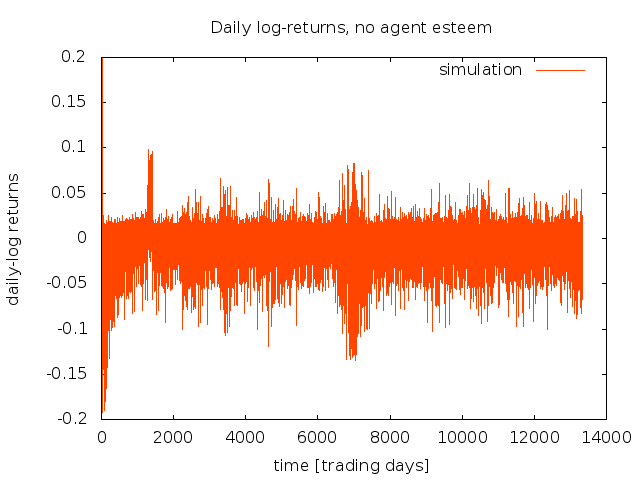
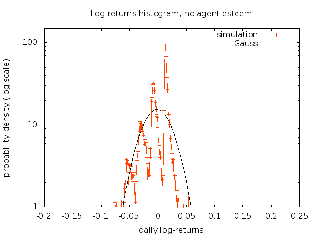
For the purpose of comparison, we have also conducted simulations for the case where the agents’ memory was extended only over one time i.e. over . For comparison, these simulations with no agents’ esteem, are shown together with simulations A and B in Figure 1, There the long-term rising and falling of trust in the foreseeing agents is somehow implicitly coded.
4 Main results
4.1 Log-returns clustering
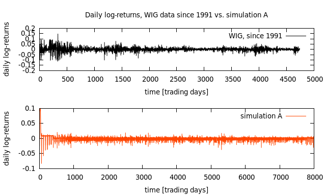
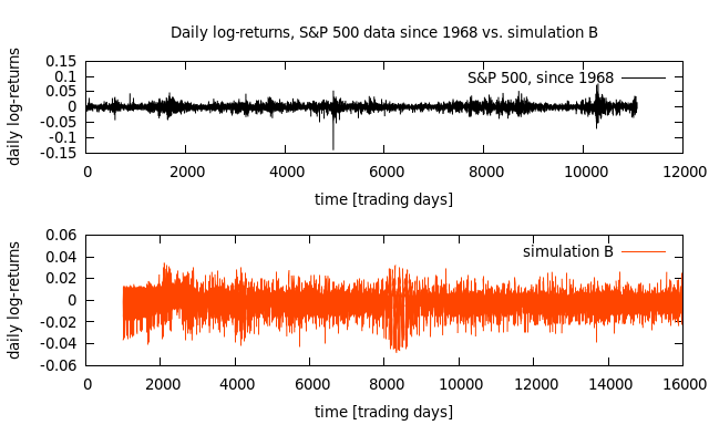
The highly non-Gaussian property of log-returns as defined by Equation (6) of log-returns time clustering is being studied in this section. The results given below, showing log-returns clustring, have been obtained by assuming 6 decision rounds as a single trading day. This behaviour directly implies the clustering of volatility (defined, e.g., as the absolute value of log-returns or their square). Our results obtained in simulations A and B, are shown in Figure 1 (both middle plots), were compared with the closing time daily empirical data for the indicies: the Warsaw Stock Index (WIG) from 1991-04-16 to 2012-01-05 (top left plot) and the Standard & Poor’s 500 index from 1968-01-01 to 2012-01-05 (top right plot) [10].
Apparently, the log-returns clusterings obtained in simulations for variograms are sufficiently distinct, although not so pronounced as for the corresponding empirical variograms. All variograms are shown in Figure 1, Notably, no periodicity is observed for the variograms despite the fact that the fundamental behaviour of investors has some periodic component. Our results occur not to be substantially affected if the system’s memory is cut to the minimal range, that is to (see the plot placed at the bottom of Figure 1).
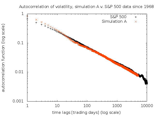
4.2 Power-law decay of autocorrelation function
The (normalized) autocorrelation function over time as a function of the time lag has been calculated as follows:
| (8) |
where is the decision round number, is the time lag, is a time average (cf. Equation (6)), and is the variance of the distribution of that log-return over time period .
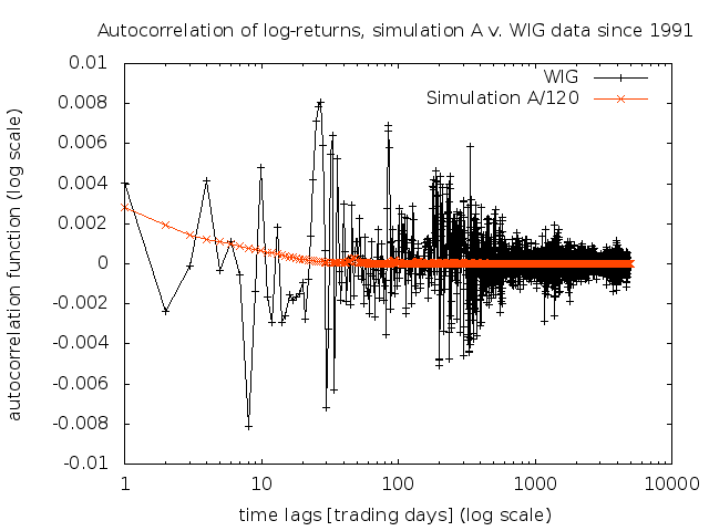
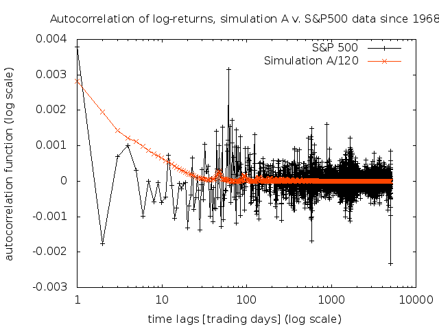
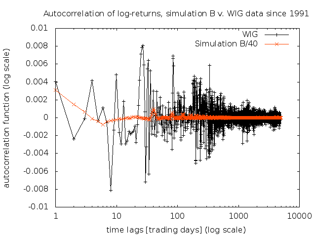
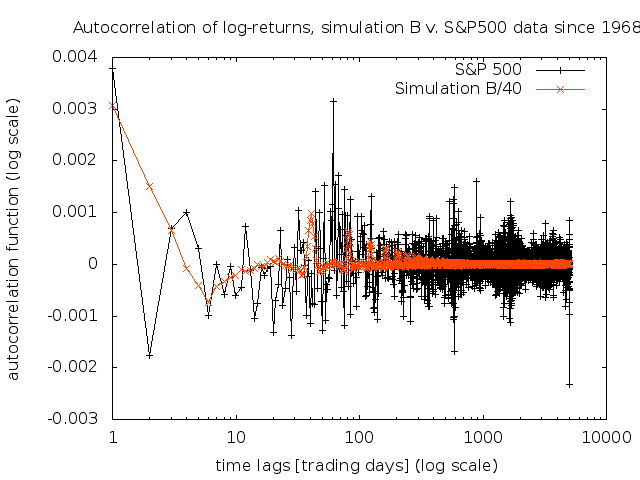
The predictions of Equation (8) are compared with empirical data in Figure 2. Despite of poor agreement, some short-term relaxations are well seen, in particular, for the S&P 500 index (bottom plots).
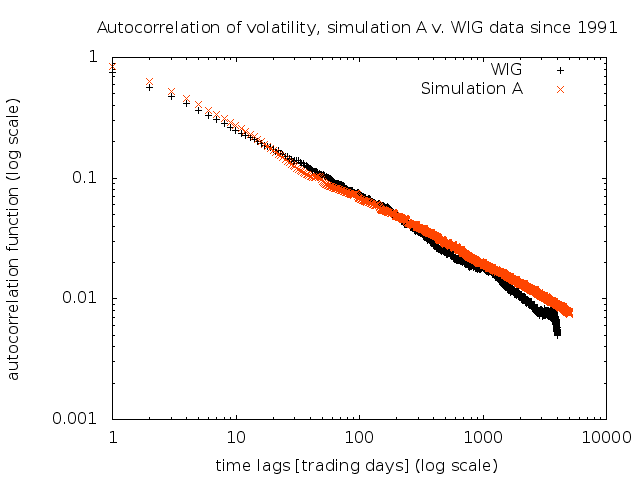
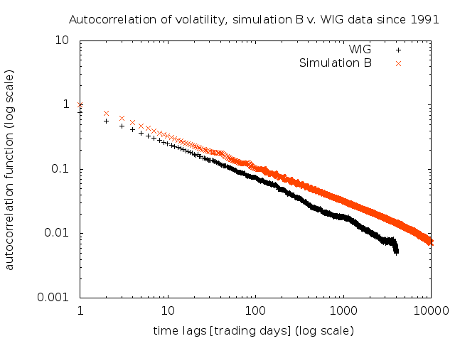
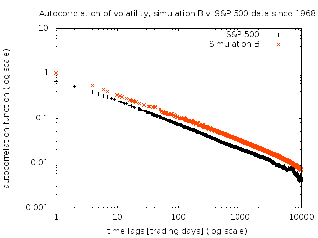
The autocorrelation function of absolute daily log-returns reveals long-term power-law relaxation versus time:
| (9) |
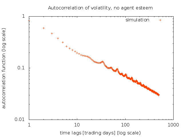
The values of exponent obtained from simulations well agree with the corresponding ones obtained from the empirical data both for WIG and S&P 500. We found the following values of exponent for the empirical data namely, and as well as for simulations and (cf. Figure 3). Exponent for simulation A agrees well with the corresponding one for WIG data and for simulation B agrees with that for S$P 500 data. Moreover, the exponent for the model without long memory of agents’ esteem (i.e. for ) equals , which is not so far placed from results obtained in simulations A and B. The results shown in Figure 3 make our model promising for studying subsequent stylized facts.
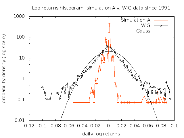
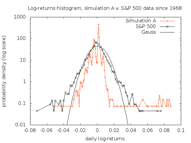
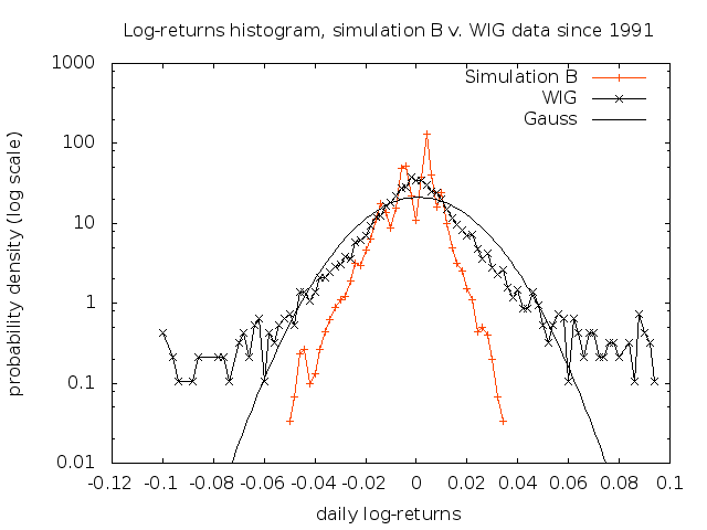
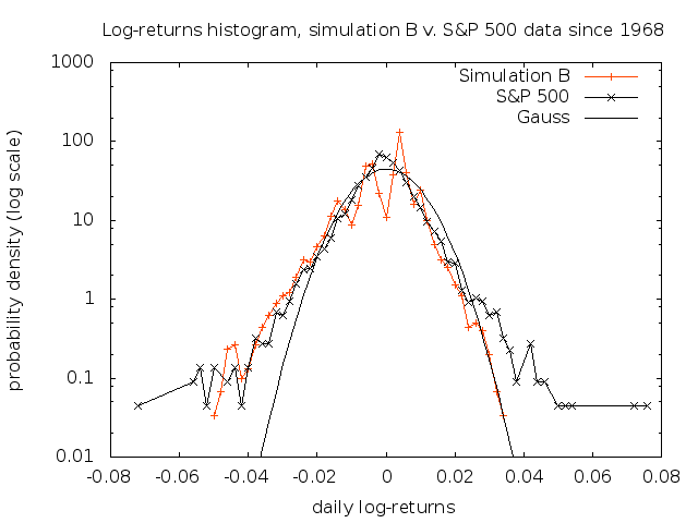
4.3 Fat-tail log-returns
Histograms for real market daily log-returns exhibit fat-tails (see Figure 4). However, the tails are thinner than the corresponding tails of the Lévy distribution. Apparently, better agreement between simulations and empirical data has been observed for the developed market described by S&P 500 than for the emerging Warsaw Stock Exchange. This stylized fact (i.e. the presence of fat-tails in daily log-returns distributions) is not reproduced if the system’s memory is assumed as .
5 Conclusions
Our modifications of the Iori model using success based strategy, which introduced intrinsically-driven herding and emotional behaviour of investors, gave satisfactory results. The following stylized facts have been reproduced:
-
•
log-returns and hence volatility clustering,
-
•
fat-tail log-return distribution,
-
•
power law autocorrelation function decay vs. time of log-returns and also quick (short-term) decay of autocorrelation function of log-returns.
It is shown that the role of a long memory of the system, that is, a growing trust in the foreseeing neighbours, is most pronounce in the case of reproducing fat-tail dostribution of log-returns.
We can conlude our (as we hope) quite representative results by the general observation that our model significantly better fits empirical data coming from stock markets of large size than from emerging markets.
Since the local field (present in Equation (2)) can be interpreted as the th agent’s utility function, a bridge between our model and utility function theories has been constructed.
References
- [1] G. Iori: A microsimulation of traders in the stock market: the role of heterogeneity, agents’ interactions and trade frictions., Journal of Economic Behaviour and Organization 49 (2), 269 (2002).
- [2] W. X. Zhou, D. Sornette: Self-fulfilling Ising Model of Financial Markets, European Physical Journal B 55, 175-181 (2007).
- [3] P. Sieczka, J. A. Hołyst: A Threshold Model of Financial Markets, Acta Phys. Pol. A 114 (3), pp. 525-530 (2008).
- [4] J. Voit: The Statistical Mechanics of Financial Markets, Springer-Verlag, Berlin-Heidelberg 2001.
- [5] T. Gubiec, R. Kutner, T. R. Werner, D. Sornette: From agent activities to financial market dynamics, 2010, PACS Nos.: 89.65.Gh, 02.50.Ey, 02.50.Ga, 05.40.Fb, 02.30.Mv.
- [6] M. Cristelli, L. Pietronero, A. Zaccaria: Critical Overview of Agent-Based Models for Economics , Proceedings of the School of Physics "E. Fermi", course CLXXVI (2010).
- [7] J. D. Farmer, D. Foley: The economy needs agent-based modelling, Nature, vol 460 (2009).
- [8] M. Denys: Badanie leptokurtyczności rozkładów modelowych i symulowanych szumów, Master thesis supervised by R. Kutner, Warszawa 2011.
- [9] J. A. Lipski: Badanie wpływu interakcji między inwestorami na dynamikę giełdy za pomocą trójstanowego modelu Isinga, Bachelor thesis supervised by Professor R. Kutner, Warszawa 2011.
-
[10]
Market data downloaded from the websiste
http://www.stooq.pl.