Linear Bandits in High Dimension and Recommendation Systems

Abstract

A large number of online services provide automated recommendations to help users to navigate through a large collection of items. New items (products, videos, songs, advertisements) are suggested on the basis of the user’s past history and –when available– her demographic profile. Recommendations have to satisfy the dual goal of helping the user to explore the space of available items, while allowing the system to probe the user’s preferences.

We model this trade-off using linearly parametrized multi-armed bandits, propose a policy and prove upper and lower bounds on the cumulative “reward” that coincide up to constants in the data poor (high-dimensional) regime. Prior work on linear bandits has focused on the data rich (low-dimensional) regime and used cumulative “risk” as the figure of merit. For this data rich regime, we provide a simple modification for our policy that achieves near-optimal risk performance under more restrictive assumptions on the geometry of the problem. We test (a variation of) the scheme used for establishing achievability on the Netflix and MovieLens datasets and obtain good agreement with the qualitative predictions of the theory we develop.

1 Introduction

Recommendation systems are a key technology for navigating through the ever-growing amount of data that is available on the Internet (products, videos, songs, scientific papers, and so on). Recommended items are chosen on the basis of the user’s past history and have to strike the right balance between two competing objectives:

Serendipity

i.e. allowing accidental pleasant discoveries. This has a positive –albeit hard to quantify– impact on user experience, in that it naturally limits the recommendations monotony. It also has a quantifiable positive impact on the systems, by providing fresh independent information about the user preferences.

Relevance

i.e. determining recommendations which are most valued by the user, given her past choices.

While this trade-off is well understood by practitioners, as well as in the data mining literature [SPUP02, ZH08, SW06], rigorous and mathematical work has largely focused on the second objective [SJ03, SRJ05, CR09, Gro09, CT10, KMO10a, KMO10b, KLT11]. In this paper we address the first objective, building on recent work on linearly parametrized bandits [DHK08, RT10, AYPS11].

In a simple model, the system recommends items $i(1),i(2),i(3),\dots$ sequentially at times $t\in\{1,2,3,\dots\}$. The item index at time $t$ is selected from a large set $i(t)\in[M]\equiv\{1,\dots,M\}$. Upon viewing (or reading, buying, etc.) item $i(t)$, the user provides feedback $y_{t}$ to the system. The feedback can be explicit, e.g. a one-to-five-stars rating, or implicit, e.g. the fraction of a video’s duration effectively watched by the user. We will assume that $y_{t}\in\mathbb{R}$, although more general types of feedback also play an important role in practice, and mapping them to real values is sometimes non-trivial.

A large body of literature has developed statistical methods to predict the feedback that a user will provide on a specific item, given past data concerning the same and other users (see the references above). A particularly successful approach uses ‘low rank’ or ‘latent space’ models. These models postulate that the rating $y_{i,u}$ provided by user $u$ on item $i$ is approximately given by the scalar product of two feature vectors $\theta_{u}$ and $x_{i}\in\mathbb{R}^{p}$ characterizing, respectively, the user and the item. In formulae

$$y_{i,u}=\langle x_{i},\theta_{u}\rangle+z_{i,u}\,,$$

where $\langle a,b\rangle\equiv\sum_{i=1}^{p}a_{i}b_{i}$ denotes the standard scalar product, and $z_{i,u}$ captures unexplained factors. The resulting matrix of ratings $y=(y_{i,u})$ is well-approximated by a rank-$p$ matrix.

The items feature vectors $x_{i}$ can be either constructed explicitly, or derived from users’ feedback using matrix factorization methods. Throughout this paper we will assume that they have been computed in advance using either one of these methods and are hence given. We will use the shorthand $x_{t}=x_{i(t)}$ for the feature vector of the item recommended at time $t$.

Since the items’ feature vectors are known in advance, distinct users can be treated independently, and we will hereafter focus on a single users, with feature vector $\theta$. The vector $\theta$ can encode demographic information known in advance or be computed from the user’s feedback. While the model can easily incorporate the former, we will focus on the most interesting case in which no information is known in advance.

We are therefore led to consider the linear bandit model

$$y_{t}=\langle x_{t},\theta\rangle+z_{t}\,,$$ (1)

where, for simplicity, we will assume $z_{t}\sim{\sf N}(0,\sigma^{2})$ independent of $\theta$, $\{x_{i}\}_{i=1}^{t}$ and $\{z_{i}\}_{i=1}^{t-1}$. At each time $t$, the recommender is given to choose a item feature vector $x_{t}\in{\cal X}_{p}\subseteq\mathbb{R}^{p}$, with ${\cal X}_{p}$ the set of feature vectors of the available items. A recommendation policy is a sequence of random variables $\{x_{t}\}_{t\geq 1}$, $x_{t}\in{\cal X}_{p}$ wherein $x_{t+1}$ is a function of the past history $\{y_{\ell},x_{\ell}\}_{1\leq\ell\leq t}$ (technically, $x_{t+1}$ has to be measurable on ${\cal F}_{t}\equiv\sigma(\{y_{\ell},x_{\ell}\}_{\ell=1}^{t})$). The system is rewarded at time $t$ by an amount equal to the user appreciation $y_{t}$, and we let $r_{t}$ denote the expected reward, i.e. $r_{t}\equiv{\mathbb{E}}(\langle x_{t},\theta\rangle)$.

As mentioned above, the same linear bandit problem was already studied in several papers, most notably by Rusmevichientong and Tsitsiklis [RT10]. The theory developed in that work, however, has two limitations that are important in the context of recommendation systems. First, the main objective of [RT10] is to construct policies with nearly optimal ‘regret’, and the focus is on the asymptotic behavior for $t$ large with $p$ constant. In this limit the regret per unit time goes to $0$. In a recommendation system, typical dimensions $p$ of the latent feature vector are about 20 to 50 [BK07, Kor08, KBV09]. If the vector $x_{i}$ include explicitly constructed features, $p$ can easily become easily much larger. As a consequence, existing theory requires at least $t\gtrsim 100$ ratings, which is unrealistic for many recommendation systems and a large number of users.

Second, the policies that have been analyzed in [RT10] are based on an alternation of pure exploration and pure exploitation. In exploration phases, recommendations are completely independent of the user profile. This is somewhat unrealistic (and potentially harmful) in practice because it would translate into a poor user experience. Consequently, we postulate the following desirable properties for a “good” policy:

1. Constant-optimal cumulative reward: For all time $t$, $\sum_{\ell=1}^{t}r_{\ell}$ is within a constant factor of the maximum achievable reward.

2. Constant-optimal regret: Let the maximum achievable reward be $r^{\rm opt}\equiv\sup_{x\in{\cal X}_{p}}\langle x,\theta\rangle$, then the ‘regret’ $\sum_{\ell=1}^{t}(r^{\rm opt}-r_{\ell})$ is within a constant of the optimal.

3. Approximate monotonicity: For any $0\leq t\leq s$, we have ${\mathbb{P}}\{\langle x_{s},\theta\rangle\geq c_{1}r_{t}\}\geq c_{2}$ for $c_{1},c_{2}$ as close as possible to $1$.

We aim, in this paper, to address the first objection in a fairly general setting. In particular, when $t$ is small, say a constant times $p$, we provide matching upper and lower bounds for the cumulative reward under certain mild assumptions on the set of arms ${\cal X}_{p}$. Under more restrictive assumptions on the set of arms ${\cal X}_{p}$, our policy can be extended to achieve near optimal regret as well. Although we will not prove a formal result of the type of Point 3, our policy is an excellent candidate in that respect.

The paper is organized as follows : in Section 2 we formally state our main results. In Section 3 we discuss further related work. Some explication on the assumptions we make on the set of arms ${\cal X}_{p}$ is provided in Section 4. In Section 5 we present numerical simulations of our policy on synthetic as well as realistic data from the Netflix and MovieLens datasets. We also compare our results with prior work, and in particular with the policy of [RT10]. Finally, proofs are given in Sections 6 and 7.

2 Main results

We denote by ${\sf Ball}(x;\rho)$ the Euclidean ball in $\mathbb{R}^{p}$ with radius $\rho$ and center $x\in\mathbb{R}^{p}$. If $x$ is the origin, we omit this argument and write ${\sf Ball}(\rho)$. Also, we denote the identity matrix as ${\rm I}_{p}$.

Our achievability results are based on the following assumption on the set of arms ${\cal X}_{p}$.

Assumption 1.

Assume, without loss of generality, ${\cal X}_{p}\in{\sf Ball}(1)$. We further assume that there exists a subset of arms ${\cal X}^{\prime}_{p}\subseteq{\cal X}_{p}$ such that:

1. For each $x\in{\cal X}^{\prime}_{p}$ there exists a distribution ${\mathbb{P}}_{x}(z)$ supported on ${\cal X}_{p}$ with ${\mathbb{E}}_{x}(z)=x$ and ${\mathbb{E}}_{x}(zz^{\sf T}){\,\succeq\,}(\gamma/p){\rm I}_{p}$, for a constant $\gamma>0$. Here ${\mathbb{E}}_{x}(\cdot)$ denotes expectation with respect to ${\mathbb{P}}_{x}$.

2. For all $\theta\in\mathbb{R}^{p}$, $\sup_{x\in{\cal X}^{\prime}_{p}}\langle x,\theta\rangle\geq\kappa\lVert{\theta}\rVert_{2}$ for some $\kappa>0$.

Examples of sets satisfying Assumption 1 and further discussion of its geometrical meaning are deferred to Section 4. Intuitively, it requires that ${\cal X}_{p}$ is ‘well spread-out’ in the unit ball ${\sf Ball}(1)$.

Following [RT10] we will also assume $\theta\in\mathbb{R}^{p}$ to be drawn from a Gaussian prior ${\sf N}(0,{\rm I}_{p}/p)$. This roughly corresponds to the assumption that nothing is known a priori about the user except the length of its feature vector $\lVert{\theta}\rVert\approx 1$. Under this assumption, the scalar product $\langle x_{1},\theta\rangle$, where $x_{1}$ is necessarily independent of $\theta$, is also Gaussian with mean $0$ and variance $1/p$ and hence $\Delta=p\sigma^{2}$ is noise-to-signal ratio for the problem. Our results are explicitly computable and apply to any value of $\Delta$. However they are constant-optimal for $\Delta$ bounded away from zero.

Let $\hat{\theta}_{t}$ be the posterior mean estimate of $\theta$ at time $t$, namely

$$\hat{\theta}_{t}\equiv\arg\min_{\theta\in\mathbb{R}^{p}}\Big{\{}\frac{1}{2\sigma^{2}}\sum_{\ell=1}^{t-1}\big{(}y_{\ell}-\langle x_{\ell},\theta\rangle\big{)}^{2}+\frac{1}{2p}\|\theta\|^{2}\Big{\}}\,.$$ (2)

A greedy policy would select the arm $x\in{\cal X}_{p}$ that maximizes the expected one-step reward $\langle x,\hat{\theta}_{t}\rangle$. As for the classical multiarmed bandit problem, we would like to combine this approach with random exploration of alternative arms. We will refer to our strategy as SmoothExplore since it combines exploration and exploitation in a continuous manner. This policy is summarized in Table 1.

Algorithm 1 SmoothExplore

1:initialize $\ell=1$, $\hat{\theta}_{1}=0$, $\hat{\theta}_{1}/\lVert{\hat{\theta}_{1}}\rVert=e_{1}$, $\Sigma_{1}={\rm I}_{p}/p$.

2:repeat

3:     Compute: $\tilde{x}_{\ell}=\arg\max_{x\in{\cal X}^{\prime}_{p}}\langle\hat{\theta}_{\ell},x\rangle$.

4:     Play: $x_{\ell}\sim{\mathbb{P}}_{\tilde{x}_{\ell}}(\cdot)$, observe $y_{t}=\langle x_{t},\theta\rangle+z_{t}$.

5:     Update: $\ell\leftarrow\ell+1$, $\hat{\theta}_{\ell}=\arg\min_{\theta\in\mathbb{R}^{p}}\frac{1}{2\sigma^{2}}\sum_{i=1}^{\ell-1}(y_{i}-\langle x_{i},\theta\rangle)^{2}+\frac{1}{2p}\lVert{\theta}\rVert^{2}$.

6:until $\ell>t$

The policy SmoothExplore uses a fixed mixture of exploration and exploitation as prescribed by the probability kernel ${\mathbb{P}}_{x}(\,\cdot\,)$. As formalized below, this is constant optimal in the data poor high-dimensional regime hence on small time horizons.

While the focus of this paper is on the data poor regime, it is useful to discuss how the latter blends with the data rich regime that arises on long time horizons. This also clarifies where the boundary between short and long time horizons sits. Of course, one possibility would be to switch to a long-time-horizon policy such as the one of [RT10]. Alternatively, in the spirit of approximate monotonicity, we can try to progressively reduce the random exploration component as $t$ increases. We will illustrate this point for the special case ${\cal X}_{p}\equiv{\sf Ball}(1)$. In that case, we introduce a special case of SmoothExplore , called BallExplore , cf. Table 2. The amount of random exploration at time $t$ is gauged by a parameter $\beta_{t}$ that decreases from $\beta_{1}=\Theta(1)$ to $\beta_{t}\to 0$ as $t\to\infty$.

Note that, for $t\leq p\Delta$, $\beta_{t}$ is kept constant with $\beta_{t}=\sqrt{2/3}$. In this regime BallExplore corresponds to SmoothExplore with the choice ${\cal X}^{\prime}_{p}=\partial{\sf Ball}(1/\sqrt{3})$ (here and below $\partial S$ denotes the boundary of a set $S$). It is not hard to check that this choice of ${\cal X}^{\prime}_{p}$ satisfies Assumption 1 with $\kappa=1/\sqrt{3}$ and $\gamma=2/3$. For further discussion on this point, we refer the reader to Section 4.

Algorithm 2 BallExplore

1:initialize $\ell=1$, $\hat{\theta}_{1}=0$, $\hat{\theta}_{1}/\lVert{\hat{\theta}_{1}}\rVert=e_{1}$, $\Sigma_{1}={\rm I}_{p}/p$, ${\sf P}^{\perp}_{1}={\rm I}_{p}-e_{1}e_{1}^{\sf T}$.

2:repeat

3:     Compute: $\tilde{x}_{\ell}=\arg\max_{x\in{\sf Ball}(1)}\langle\hat{\theta}_{\ell},x\rangle=\hat{\theta}_{\ell}/\lVert{\hat{\theta}_{\ell}}\rVert$, $\beta_{\ell}=\sqrt{2/3}\min(p\Delta/\ell,1)^{1/4}$.

4:     Play: $x_{t}=\sqrt{1-\beta_{\ell}^{2}}\tilde{x}_{\ell}+\beta_{\ell}{\sf P}^{\perp}_{\ell}u_{\ell}$, where $u_{\ell}$ is a uniformly sampled unit vector, independent of the past.

5:     Observe: $y_{t}=\langle x_{t},\theta\rangle+z_{t}$.

6:     Update: $\ell\leftarrow\ell+1$, $\hat{\theta}_{\ell}=\arg\min_{\theta\in\mathbb{R}^{p}}\frac{1}{2\sigma^{2}}\sum_{i=1}^{\ell-1}(y_{i}-\langle x_{i},\theta\rangle)^{2}+\frac{1}{2p}\lVert{\theta}\rVert^{2}$, ${\sf P}^{\perp}_{\ell}={\rm I}_{p}-\hat{\theta}_{\ell}\hat{\theta}_{\ell}^{\sf T}/\lVert{\hat{\theta}_{\ell}}\rVert^{2}$.

7:until $\ell>t$

Our main result characterizes the cumulative reward

$$R_{t}\equiv\sum_{\ell=1}^{t}r_{t}=\sum_{\ell=1}^{t}{\mathbb{E}}\{\langle x_{\ell},\theta\rangle\}\,.$$

Theorem 1.

Consider the linear bandits problem with $\theta\sim{\sf N}(0,{\rm I}_{p\times p}/p)$, $x_{t}\in{\cal X}_{p}\subseteq{\sf Ball}(1)$ satisfying Assumption 1, and $p\sigma^{2}=\Delta$. Further assume that $p\geq 2$ and $p\Delta\geq 2$.

Then there exists a constant $C_{1}=C_{1}(\kappa,\gamma,\Delta)$ bounded for $\kappa,\gamma$ and $\Delta$ bounded away from zero, such that SmoothExplore achieves, for $1<t\leq p\Delta$, cumulative reward

$$\quad R_{t} \geq C_{1}\,t^{3/2}p^{-1/2}.$$

Further, the cumulative reward of any strategy is bounded for $1\leq t\leq p\Delta$ as:

$$\quad R_{t}\leq C_{2}\,t^{3/2}p^{-1/2}\,.$$

We may take the constants $C_{1}(\kappa,\gamma,\Delta)$ and $C_{2}(\Delta)$ to be:

$$C_{1}=\frac{\kappa\sqrt{\Delta}\,C(\gamma,\Delta)}{24\,\alpha(\gamma,\Delta)}, \qquad C_{2}=\frac{2}{3\sqrt{\Delta}},$$

$$\textrm{where }\quad C(\gamma,\Delta)=\frac{\gamma}{4(\Delta+1)}, \qquad\alpha(\gamma,\Delta)=1+\left[3\log\left(\frac{96}{\Delta\,C(\gamma,\Delta)}\right)\right]^{1/2}.$$

In the special case where ${\cal X}_{p}={\sf Ball}(1)$, we have the following result demonstrating that BallExplore has near-optimal performance in the long time horizon as well.

Theorem 2.

Consider the linear bandits problem with $\theta\sim{\sf N}(0,{\rm I}_{p\times p}/p)$ with the set of arms ${\cal X}_{p}$ is the unit ball, i.e. ${\sf Ball}(1)$. Assume, $p\geq 2$ and $p\Delta\geq 2$. Then BallExplore achieves for all $t>p\Delta$:

$$R_{t} \geq r^{\rm opt}\,t-C_{3}\,(pt)^{1/2+\omega(p)}\,.$$

where:

$$\omega(p)=1/(2(p+2)), \qquad C_{3}(\Delta)=70\left(\frac{\Delta+1}{\sqrt{\Delta}}\right).$$

For $t>p\Delta$, we can obtain a matching upper bound by a simple modification of the arguments in [RT10].

Theorem 3 (Rusmevichientong and Tsitsiklis).

Under the described model, the cumulative reward of any policy is bounded as follows

$$\mbox{for }t>p\Delta,\quad R_{t}\leq r^{\rm opt}\,t-\sqrt{pt\Delta}+\frac{p\Delta}{2}\,.$$

The above results characterize a sharp dichotomy between a low-dimensional, data rich regime for $t>p\Delta$ and a high-dimensional, data poor regime for $t\leq p\Delta$. In the first case classical theory applies: the reward approaches the oracle performance with a gap of order $\sqrt{pt}$. This behavior is in turn closely related to central limit theorem scaling in asymptotic statistics. Notice that the scaling with $t$ of our upper bound on the risk of BallExplore for large $t$ is suboptimal, namely $(pt)^{1/2+\omega(p)}$. Since however $\omega(p)=\Theta(1/p)$ the difference can be seen only on exponential time scales $t\geq\exp\{\Theta(p)\}$ and is likely to be irrelevant for moderate to large values $p$ (see Section 5 for a demonstration). It is an open problem to establish the exact asymptotic scaling of BallExplore .

In the high-dimensional, data poor regime $t\leq p\Delta$, the number of observations is smaller than the number of model parameters and the vector $\theta$ can only be partially estimated. Nevertheless, such partial estimate can be exploited to produce a cumulative reward scaling as $t^{3/2}p^{-1/2}$. In this regime performances are not limited by central limit theorem fluctuations in the estimate of $\theta$. The limiting factor is instead the dimension of the parameter space that can be effectively explored in $t$ steps.

In order to understand this behavior, it is convenient to consider the noiseless case $\sigma=0$. This is a somewhat degenerate case that, although not covered by the above theorem, yields useful intuition. In the noiseless case, acquiring $t$ observations $y_{1}$, …$y_{t}$ is equivalent to learning the projection of $\theta$ on the $t$-dimensional subspace spanned by $x_{1},\dots,x_{t}$. Equivalently, we learn $t$ coordinates of $\theta$ in a suitable basis. Since the mean square value of each component of $\theta$ is $1/p$, this yields an estimate of $\hat{\theta}_{t}$ (the restriction to these coordinates) with ${\mathbb{E}}\|\hat{\theta}_{t}\|^{2}_{2}=t/p$. By selecting $x_{t}$ in the direction of $\hat{\theta}_{t}$ we achieve instantaneous reward $r_{t}\approx\sqrt{t/p}$ and hence cumulative reward $R_{t}=\Theta(t^{3/2}p^{-1/2})$ as stated in the theorem.

3 Related work

Auer in [Aue02] first considered a model similar to ours, wherein the parameter $\theta$ and noise $z_{t}$ are bounded almost surely. This work assumes ${\cal X}_{p}$ finite and introduces an algorithm based on upper confidence bounds. Dani et al. [DHK08] extended the policy of [Aue02] for arbitrary compact decision sets ${\cal X}_{p}$. For finite sets, [DHK08] prove an upper bound on the regret that is logarithmic in its cardinality $|{\cal X}_{p}|$, while for continuous sets they prove an upper bound of $O(\sqrt{pt}\log^{3/2}t)$. This result was further improved by logarithmic factors in [AYPS11]. The common theme throughout this line of work is the use of upper confidence bounds and least-squares estimation. The algorithms typically construct ellipsoidal confidence sets around the least-squares estimate $\hat{\theta}$ which, with high probability, contain the parameter $\theta$. The algorithm then chooses optimistically the arm that appears the best with respect to this ellipsoid. As the confidence ellipsoids are initialized to be large, the bounds are only useful for $t\gg p$. In particular, in the high-dimensional data-poor regime $t=O(p)$, the bounds typically become trivial. In light of Theorem 3 this is not surprising. Even after normalizing the noise-to-signal ratio while scaling the dimension, the $O(\sqrt{pt})$ dependence of the risk is relevant only for large time scales of $t\geq p\Delta$. This is the regime in which the parameter $\theta$ has been estimated fairly well.

Rusmevichientong and Tsitsiklis [RT10] propose a phased policy which operates in distinct phases of learning the parameter $\theta$ and earning based on the current estimate of $\theta$. Although this approach yields order optimal bounds for the regret, it suffers from the same shortcomings as confidence-ellipsoid based algorithms. In fact, [RT10] also consider a more general policy based on confidence bounds and prove a $O(\sqrt{pt}\log^{3/2}t)$ bound on the regret.

Our approach to the problem is significantly different and does not rely on confidence bounds. It would be interesting to understand whether the techniques developed here can be use to improve the confidence bounds method.

4 On Assumption 1

The geometry of the set of arms ${\cal X}_{p}$ is an important factor in the in the performance of any policy. For instance, [RT10], [DHK08] and [AYPS11] provide “problem-dependent” bounds on the regret incurred in terms of the difference between the reward of the optimal arm and the next-optimal arm. This characterization is reasonable in the long time horizon: if the posterior estimate $\hat{\theta}_{t}$ of the feature vector $\theta$ coincided with $\theta$ itself, only the optimal arm would matter. Since the posterior estimate converges to $\theta$ in the limit of large $t$, the local geometry of ${\cal X}_{p}$ around the optimal arm dictates the asymptotic behavior of the regret.

In the high-dimensional, short-time regime, the global geometry of ${\cal X}_{p}$ plays instead a crucial role. This is quantified in our results through the parameters $\kappa$ and $\gamma$ appearing in Assumption 1. Roughly speaking, this amounts to requiring that ${\cal X}_{p}$ is ‘spread out’ in the unit ball. It is useful to discuss this intuition in a more precise manner. For the proofs of statements in this section we refer to Appendix A.

A simple case is the one in which the arm set contains a ball.

Lemma 4.1.

If ${\sf Ball}(\rho)\subseteq{\cal X}_{p}\subseteq{\sf Ball}(1)$, then ${\cal X}_{p}$ satisfies Assumption 1 with $\kappa=\rho/\sqrt{3}$, $\gamma=2\rho^{2}/3$.

The last lemma does not cover the interesting case in which ${\cal X}_{p}$ is finite. The next result shows however that, for Assumption 1.2 to hold it is sufficient that the closure of the convex hull of ${\cal X}^{\prime}_{p}$, denoted by $\overline{\rm conv}({\cal X}^{\prime}_{p})$, contains a ball.

Proposition 4.2.

Assumption 1.2 holds if and only if ${\sf Ball}(\kappa)\subseteq\overline{\rm conv}({\cal X}^{\prime}_{p})$.

In other words, Assumption 1.2 is satisfied if ${\cal X}^{\prime}_{p}$ is ‘spread out’ in all directions around the origin.

Finally, we consider a concrete example with ${\cal X}_{p}$ finite. Let $x_{1},x_{2},\dots,x_{M}$ to be i.i.d. uniformly random in ${\sf Ball}(1)$. We then refer to the set of arms ${\cal X}_{p}\equiv\{x_{1},x_{2},\dots,x_{M}\}$ as to a uniform cloud.

Proposition 4.3.

A uniform cloud ${\cal X}_{p}$ in dimension $p\geq 20$ satisfies Assumption 1 with $M=8^{p}$, $\kappa=1/4$ and $\gamma=1/32$ with probability larger than $1-2\exp(-p)$.

5 Numerical results

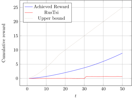
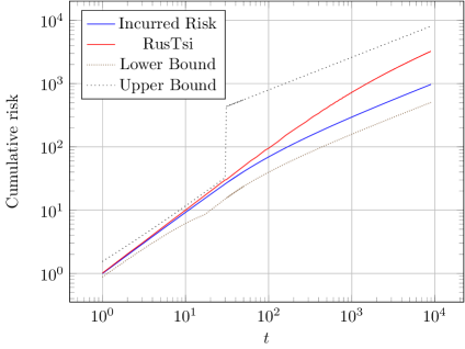
Figure 1: Left frame: Cumulative reward $R_{t}$ in the data poor regime $t\lesssim 2\,p\Delta$ (here $p=30$, $\Delta=1$) as obtained through numerical simulations over synthetic data, together with analytical upper bound. Right frame: Cumulative risk in the data rich regime $t\gg p\Delta$ (again, $p=30$, $\Delta=1$).

We will mainly compare our results with those of [RT10] since the results of that paper directly apply to the present problem. The authors proposed a phased exploration/exploitation policy, wherein they separate the phases of learning the parameter $\theta$ (exploration) and earning reward based on the current estimate of $\theta$ (exploitation).

In Figure 1 we plot the cumulative reward and the cumulative risk incurred by our policy and the phased policy, as well as analytical bounds thereof. We generated $\theta\sim{\sf N}(0,{\rm I}_{p})$ randomly for $p=30$, and produced observations $y_{t}$, $t\in\{1,2,3,\dots\}$ according to the general model (1) with $\Delta=p\sigma^{2}=1$ and arm set ${\cal X}_{p}={\sf Ball}(1)$. The curves presented here are averages over $n=5000$ realizations and statistical fluctuations are negligible.

The left frame illustrates the performance of SmoothExplore in the data poor (high-dimensional) regime $t\lesssim 2\,p\Delta$. We compare the cumulative reward $R_{t}$ as achieved in simulations, with that of the phased policy of [RT10] and with the theoretical upper bound of Theorem 1 (and Theorem 3 for $t>p\Delta$). In the right frame we consider instead the data rich (low-dimensional) regime $t\gg p\Delta$. In this case it is more convenient to plot the cumulative risk $tr^{\rm opt}-R_{t}$. We plot the curves corresponding to the ones in the left frame, as well as the upper bound (lower bound on the reward) from Theorems 1 and 2.

Note that the $O(\sqrt{pt})$ behavior of the risk of the phased policy can be observed only for $t\gtrsim 1000$. On the other hand, our policy displays the correct behavior for both time scales. The extra $\omega(p)=\Theta(1/p)$ factor in the exponent yields a multiplicative factor larger than $2$ only for $t\geq 2^{2(p+2)}\approx 2\cdot 10^{19}$.

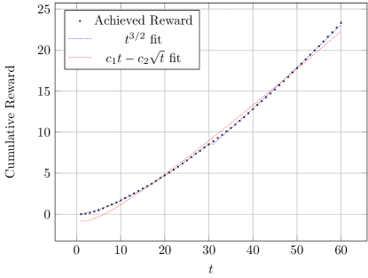
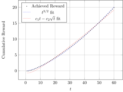
Figure 2: Results using the Netflix (left frame) and MovieLens 1M (right frame) datasets. SmoothExplore is effective in learning the user’s preferences and is well described by the predicted behavior of Theorem 1.

The above set of numerical experiments used ${\cal X}_{p}={\sf Ball}(1)$. For applications to recommendation systems, ${\cal X}_{p}$ is in correspondence with a certain catalogue of achievable products or contents. In particular, ${\cal X}_{p}$ is expected to be finite. It is therefore important to check how does SmoothExplore perform for a realistic sets of arms. We plot results obtained with the Netflix Prize dataset and the MovieLens 1M dataset in Figure 2. Here the feature vectors $x_{i}$’s for movies are obtained using the matrix completion algorithm of [KMO10b]. The user parameter vectors $\theta_{u}$ were obtained by regressing the rating against the movie feature vectors (the average user rating $a_{u}$ was subtracted). Similar to synthetic data, we took $p=30$. Regression also yields an estimate for the noise variance which is assumed known in the algorithm. We then simulated an interactive scenario by postulating that the rating of user $u$ for movie $i$ is given by

$$\widetilde{y}_{i,u}={\sf Quant}(a_{u}+\langle x_{,}\theta_{u}\rangle)\,,$$

where ${\sf Quant}(z)$ quantizes $z$ to to $\{1,2,\cdots,5\}$ (corresponding to a one-to-five star rating). The feedback used for our simulation is the centered rating $y_{i,u}=\widetilde{y}_{i,u}-a_{u}$.

We implement a slightly modified version of SmoothExplore for these simulations. At each time we compute the ridge regression estimate of the user feature vector $\hat{\theta}_{t}$ as before and choose the “best” movie $\tilde{x}_{t}=\arg\max_{x\in{\cal X}_{p}}\langle x,\hat{\theta}_{t}\rangle$ assuming our estimate is error free. We then construct the ball in $\mathbb{R}^{p}$ with center $\tilde{x}_{t}$ and radius $\beta_{t}$. We list all the movies whose feature vectors fall in this ball, and recommend a uniformly randomly chosen one in this list.

Classical bandit theory implies the reward behavior is of the type $c_{1}t-c_{2}\sqrt{t}$ where $c_{1}$ and $c_{2}$ are (dimension-dependent) constants. Figure 2 presents the best fit of this type for $t\lesssim 2p$. The description appears to be qualitatively incorrect in this regime. Indeed, in this regime, the reward behavior is better explained by a $c_{3}t^{3/2}$ curve. These results suggest that our policy is fairly robust to the significant modeling uncertainty inherent in the problem. In particular, the fact that the “noise” encountered in practice is manifestly non-Gaussian does not affect the qualitative predictions of Theorem 1.

A full validation of our approach would require an actual interactive realization of a recommendation system [DM13]. Unfortunately, such validation cannot be provided by existing datasets, such as the ones used here. A naive approach would be to use the actual ratings as the feedback $y_{iu}$, but this suffers from many shortcomings. First of all, each user rates a sparse subset (of the order of $100$ movies) of the whole database of movies, and hence any policy to be tested would be heavily constrained and distorted. Second, the set of rated movies is a biased subset (since it is selected by the user itself).

6 Proof of Theorem 1

We begin with some useful notation. Define the $\sigma$-algebra ${\cal F}_{t}\equiv\sigma(\{y_{\ell},x_{\ell}\}_{\ell=1}^{t})$. Also let $\mathcal{G}_{t}\equiv\sigma(\{y_{\ell}\}_{\ell=1}^{t-1},\{x_{\ell}\}_{\ell=1}^{t})$. We let $\hat{\theta}_{t}$ and $\Sigma_{t}$ denote the posterior mean and covariance of $\theta$ given $t-1$ observations. Since $\theta$ is Gaussian and the observations are linear, it is a standard result that these can be computed as:

$$\Sigma_{t} \equiv{\rm Cov}(\theta|{\cal F}_{t-1})=\left(p{\rm I}_{p}+\frac{1}{\sigma^{2}}\sum_{\ell=1}^{t-1}x_{\ell}x_{\ell}^{\sf T}\right)^{-1}$$

$$\hat{\theta}_{t} \equiv{\mathbb{E}}(\theta|{\cal F}_{t-1})=\Sigma_{t}\left(\sum_{\ell=1}^{t-1}\frac{y_{\ell}}{\sigma^{2}}x_{\ell}\right).$$

Note that since $\theta$ is Gaussian and the measurements are linear the posterior mean coincides with the maximum likelihood estimate for $\theta$. This ensures our notation is consistent.

6.1 Upper bound on reward

At time $\ell$, the expected reward $r_{\ell}={\mathbb{E}}(\langle x_{\ell},\theta\rangle)\leq{\mathbb{E}}(\lVert{\hat{\theta}_{\ell}}\rVert)\leq\bigl{[}{\mathbb{E}}(\lVert{\hat{\theta}_{\ell}}\rVert^{2})\bigr{]}^{1/2}$, where the first inequality follows from Cauchy-Schwarz, that $\hat{\theta}_{\ell}$ is unbiased and that $\lVert{x_{\ell}}\rVert\leq 1$. Since $1={\mathbb{E}}(\lVert{\theta}\rVert^{2})={\mathbb{E}}(\lVert{\hat{\theta}_{\ell}}\rVert^{2})+{\mathbb{E}}({\sf{Tr}}{\Sigma_{\ell}})$:

$$r_{\ell}^{2}\leq 1-{\mathbb{E}}\left({\sf{Tr}}(\Sigma_{\ell})\right).$$ (3)

We have, applying Jensen’s inequality and further simplification:

$${\mathbb{E}}{\sf{Tr}}(\Sigma_{\ell}) \geq p^{2}/{\mathbb{E}}({\sf{Tr}}(\Sigma_{\ell}^{-1}))$$

$$=p^{2}/{\mathbb{E}}{\sf{Tr}}\left(p{\rm I}_{p}+\frac{1}{\sigma^{2}}\sum_{j=1}^{\ell-1}x_{j}x_{j}^{\sf T}\right)$$

$$\geq\left(1+\frac{\ell-1}{p^{2}\sigma^{2}}\right)^{-1}.$$

Using this to bound the right hand side of Eq. (3)

$$r_{\ell}^{2} \leq 1-\frac{1}{1+(\ell-1)/(p\sigma)^{2}}$$

$$=\frac{(\ell-1)/p}{(\ell-1)/p+{p\sigma^{2}}}$$

$$\leq\frac{1}{p\sigma^{2}}\frac{\ell-1}{p}.$$

The cumulative reward can then be bounded as follows:

$$\sum_{\ell=1}^{t}r_{\ell} \leq\frac{1}{\sqrt{p\sigma^{2}}}\sum_{\ell=1}^{t}\sqrt{\frac{\ell-1}{p}}$$

$$\leq\frac{2}{3\sqrt{p\sigma^{2}}}t^{3/2}p^{-1/2}$$

$$=C_{2}(\Delta)t^{3/2}p^{-1/2}.$$

Here we define $C_{2}(\Delta)\equiv 2/3\sqrt{\Delta}$.

6.2 Lower bound on reward

We compute the expected reward earned by SmoothExplore at time $t$ as:

$$r_{t} ={\mathbb{E}}(\langle x_{t},\theta\rangle)$$

$$={\mathbb{E}}({\mathbb{E}}(\langle x_{t},\theta\rangle|\mathcal{G}_{t-1}))$$

$$={\mathbb{E}}({\mathbb{E}}(\langle x_{t},\hat{\theta}_{t}\rangle|\mathcal{G}_{t-1}))$$

$$={\mathbb{E}}(\langle\tilde{x}_{t},\hat{\theta}_{t}\rangle)$$

$$\geq\kappa\,{\mathbb{E}}(\lVert{\hat{\theta}_{t}}\rVert).$$ (4)

The following lemma guarantees that $\lVert{\hat{\theta}_{t}}\rVert$ is $\Omega(\sqrt{t})$.

Lemma 6.1.

Under the conditions of Theorem 1 we have, for all $t>1$:

$${\mathbb{E}}\lVert{\hat{\theta}_{t}}\rVert \geq C^{\prime}(\gamma,\Delta)t^{1/2}p^{-1/2}.$$

Here:

$$C^{\prime}(\gamma,\Delta) =\frac{1}{2}\frac{C(\gamma,\Delta)}{\alpha(\gamma,\Delta)}\sqrt{\frac{\Delta}{8}},$$

$$\textrm{where }\quad C(\gamma,\Delta) =\frac{\gamma}{4(\Delta+1)}$$

$$\alpha(\gamma,\Delta) =1+\left[3\log\left(\frac{96}{\Delta C(\gamma,\Delta)}\right)\right]^{1/2}.$$

Using this lemma we proceed by bounding the right side of Eq. (6.2):

$$r_{t} \geq\kappa C^{\prime}\sqrt{\frac{t-1}{p}}.$$

Computing cumulative reward $R_{t}$ we have:

$$R_{t} =\sum_{\ell=1}^{t}r_{\ell}$$

$$\geq\sum_{\ell=1}^{t}\kappa C^{\prime}\sqrt{\frac{\ell-1}{p}}$$

$$\geq\kappa C^{\prime}\int_{0}^{t-1}\sqrt{\frac{\nu}{p}}\mathrm{d}\nu$$

$$\geq\frac{2}{3}\kappa C^{\prime}(t-1)^{3/2}p^{-1/2}$$

$$\geq\frac{\kappa C^{\prime}}{3\sqrt{2}}t^{3/2}p^{-1/2}.$$

Thus, letting $C_{1}(\kappa,\gamma,\Delta)=\kappa C^{\prime}(\gamma,\Delta)/3\sqrt{2}$, we have the required result.

6.3 Proof of Lemma 6.1

In order to prove that ${\mathbb{E}}(\lVert{\hat{\theta}_{t}}\rVert)=\Omega(\sqrt{t})$, we will first show that ${\mathbb{E}}(\lVert{\hat{\theta}_{t}}\rVert^{2})$ is $\Omega(t)$. Then we prove that $\lVert{\hat{\theta}_{t}}\rVert$ is sub-gaussian, and use this to arrive at the required result.

Lemma 6.2 (Growth of Second Moment).

Under the conditions of Theorem 1:

$${\mathbb{E}}{\lVert{\hat{\theta}_{t}}\rVert^{2}}\geq C(\Delta,\gamma)\frac{t-1}{p},$$

where

$$C(\Delta,\gamma)=\frac{\gamma}{4(\Delta+1)}.$$

Proof.

We rewrite $\hat{\theta}_{t}$ using the following inductive form:

$$\hat{\theta}_{t+1}=\hat{\theta}_{t}+\Sigma_{t+1}\left(\frac{1}{\sigma^{2}}x_{t}x_{t}^{\sf T}\right)v_{t}+\Sigma_{t+1}\frac{z_{t}}{\sigma^{2}}x_{t}.$$ (5)

Here $v_{t}\equiv\theta-\hat{\theta}_{t}$ is a random zero mean vector. Conditional on ${\cal F}_{t-1}$, $v_{t}$ is distributed as ${\sf N}(0,\Sigma_{t})$ and is independent of $x_{t}$ and $z_{t}$. Recall that the $\sigma$-algebra $\mathcal{G}_{t}=\sigma(\{y_{\ell}\}_{\ell=1}^{t-1},\{x_{\ell}\}_{\ell=1}^{t})\supseteq{\cal F}_{t-1}$. Then we have:

$${\mathbb{E}}(\lVert{\hat{\theta}_{t+1}}\rVert{}^{2}|{\mathcal{G}}_{t}) =\lVert{\hat{\theta}_{t}}\rVert{}^{2}+\frac{1}{\sigma^{4}}{\mathbb{E}}\left[v_{t}^{\sf T}\left(\Sigma_{t+1}x_{t}x_{t}^{\sf T}\right)^{\sf T}\left(\Sigma_{t+1}x_{t}x_{t}^{\sf T}\right)v_{t}\big{|}{\mathcal{G}}_{t}\right]+\frac{1}{\sigma^{4}}{\mathbb{E}}\left[z_{t}^{2}|{\mathcal{G}}_{t}\right]\left(\Sigma_{t+1}x_{t}\right)^{\sf T}\left(\Sigma_{t+1}x_{t}\right).$$ (6)

The cross terms cancel since $v_{t}$ and $z_{t}$ conditionally on ${\mathcal{G}}_{t}$ are independent and zero mean. The expectation in the second term can be reduced as follows:

$${\mathbb{E}}\left[v_{t}^{\sf T}\left(\Sigma_{t+1}x_{t}x_{t}^{\sf T}\right)^{\sf T}\left(\Sigma_{t+1}x_{t}x_{t}^{\sf T}\right)v_{t}\big{|}{\mathcal{G}}_{t}\right] ={\sf{Tr}}\left[\left(\Sigma_{t+1}x_{t}x_{t}^{\sf T}\right)\Sigma_{t}\left(\Sigma_{t+1}x_{t}x_{t}^{\sf T}\right)^{\sf T}\right]$$

$$={\sf{Tr}}\left[\left(\Sigma_{t+1}x_{t}x_{t}^{\sf T}\right)\Sigma_{t}\left(x_{t}x_{t}^{\sf T}\Sigma_{t+1}\right)\right]$$

$$=(x_{t}^{\sf T}\Sigma_{t}x_{t}){\sf{Tr}}\left[\Sigma_{t+1}x_{t}x_{t}^{\sf T}\Sigma_{t+1}\right]$$

$$=\left(x_{t}^{\sf T}\Sigma_{t}x_{t}\right)\left(x_{t}^{\sf T}\Sigma_{t+1}^{2}x_{t}\right).$$

The third term can be seen to be:

$${\mathbb{E}}\left[z_{t}^{2}|{\mathcal{G}}_{t}\right]\left(\Sigma_{t+1}x_{t}\right)^{\sf T}\left(\Sigma_{t+1}x_{t}\right) =\sigma^{2}x_{t}^{\sf T}\Sigma_{t+1}^{2}x_{t}.$$

Thus we have, continuing Eq. (6):

$${\mathbb{E}}(\lVert{\hat{\theta}_{t+1}}\rVert{}^{2}|{\mathcal{G}}_{t}) =\lVert{\hat{\theta}_{t}}\rVert{}^{2}+\frac{1}{\sigma^{4}}\left(\sigma^{2}+x_{t}^{\sf T}\Sigma_{t}x_{t}\right)\left(x_{t}^{\sf T}\Sigma_{t+1}^{2}x_{t}\right).$$ (7)

Since $\Sigma_{t+1}=\left(\Sigma_{t}^{-1}+\frac{1}{\sigma^{2}}x_{t}x_{t}^{\sf T}\right)^{-1}=\Sigma_{t}-\Sigma_{t}x_{t}x_{t}^{\sf T}\Sigma_{t}/(\sigma^{2}+x_{t}^{\sf T}\Sigma_{t}x_{t})$, some calculation yields that:

$$x_{t}^{\sf T}\Sigma_{t+1}^{2}x_{t}=\frac{\sigma^{4}\left(x_{t}^{\sf T}\Sigma_{t}^{2}x_{t}\right)}{\left(\sigma^{2}+x_{t}^{\sf T}\Sigma_{t}x_{t}\right)^{2}}.$$

Thus Eq. (7) reduces to

$${\mathbb{E}}(\lVert{\hat{\theta}_{t+1}}\rVert{}^{2}|{\mathcal{G}}_{t}) =\lVert{\hat{\theta}_{t}}\rVert{}^{2}+\frac{x_{t}^{\sf T}\Sigma_{t}^{2}x_{t}}{\sigma^{2}+x_{t}^{\sf T}\Sigma_{t}x_{t}}.$$ (8)

We now bound the additive term in Eq. (8). We know that $\Sigma_{t}{\,\preceq\,}{\rm I}/p$ (the prior covariance), thus $x_{t}^{\sf T}\Sigma_{t}x_{t}\leq 1/p$ since $x_{t}\in{\cal X}_{p}\subseteq{\sf Ball}(1)$. Hence the denominator in Eq. (8) is upper bounded by $\sigma^{2}+1/p$. To bound the numerator:

$${\mathbb{E}}[x_{t}^{\sf T}\Sigma_{t}^{2}x_{t}|{\mathcal{F}}_{t-1}] ={\mathbb{E}}[{\sf{Tr}}(\Sigma_{t}^{2}x_{t}x_{t}^{\sf T})|{\mathcal{F}}_{t-1}]$$

$$={\sf{Tr}}[\Sigma_{t}^{2}{\mathbb{E}}(x_{t}x_{t}^{\sf T}|{\mathcal{F}}_{t-1})]$$

$$\geq\frac{\gamma}{p}{\sf{Tr}}(\Sigma_{t}^{2}),$$

since ${\mathbb{E}}_{\tilde{x}_{t}}(x_{t}x_{t}^{\sf T}){\,\succeq\,}(\gamma/p){\rm I}_{p}$ by Assumption 1. Using this in Eq. (8), we take expectations to get:

$${\mathbb{E}}(\lVert{\hat{\theta}_{t+1}}\rVert{}^{2}) \geq{\mathbb{E}}(\lVert{\hat{\theta}_{t}}\rVert{}^{2})+\frac{\gamma}{\Delta+1}{\mathbb{E}}[{\sf{Tr}}(\Sigma_{t}^{2})].$$ (9)

Considering the second term in Eq. (9):

$${\mathbb{E}}[{\sf{Tr}}(\Sigma_{t}^{2})] \geq p\,{\mathbb{E}}[\det(\Sigma_{t}^{2})^{1/p}]$$

$$=p\,{\mathbb{E}}\left[\left(\prod_{j=1}^{p}\frac{1}{p+\lambda_{j}/\sigma^{2}}\right)^{2/p}\right],$$

where $\lambda_{j}$ is the $j^{\text{th}}$ eigenvalue of $\sum_{\ell=1}^{t-1}x_{\ell}x_{\ell}^{\sf T}$. Continuing the chain of inequalities:

$${\mathbb{E}}[{\sf{Tr}}(\Sigma_{t}^{2})] \geq\frac{1}{p}\,{\mathbb{E}}\left[\prod_{j=1}^{p}\left(1+\frac{\lambda_{j}}{\Delta}\right)^{-2/p}\right]$$

$$\geq\frac{1}{p}\,{\mathbb{E}}\left[\prod_{j=1}^{p}\exp\left(-\frac{2\lambda_{j}}{p\Delta}\right)\right]$$

$$=\frac{1}{p}\,{\mathbb{E}}\left[\exp\left\{-\frac{2}{p\Delta}{\sf{Tr}}\Big{(}\sum_{\ell=1}^{t}x_{\ell}x_{\ell}^{\sf T}\Big{)}\right\}\right]$$

$$\geq\frac{1}{p}\exp\left\{-\frac{2(t-1)}{p\Delta}\right\},$$

where the last inequality follows from the fact that $x_{\ell}\in{\sf Ball}(1)$ for each $\ell$. Combining this with Eq. (9) gives:

$${\mathbb{E}}(\lVert{\hat{\theta}_{t+1}}\rVert{}^{2} \geq{\mathbb{E}}(\lVert{\hat{\theta}_{t}}\rVert^{2})+\frac{\gamma}{\Delta+1}\frac{1}{p}\exp\left\{{-\frac{2(t-1)}{p\Delta}}\right\}.$$ (10)

Summing over $t$ this implies:

$${\mathbb{E}}[\lVert{\hat{\theta}_{t}}\rVert^{2}] \geq\frac{\gamma}{p(\Delta+1)}\frac{1-\exp\{2(t-1)/p\Delta\}}{1-\exp\{-2/p\Delta\}}$$

$$\geq\frac{\gamma\Delta}{2(\Delta+1)}(1-\exp\{-2(t-1)/p\Delta\})$$

$$\geq\frac{\gamma}{2(\Delta+1)}\left(1-\exp\{-2(p\Delta-1)/p\Delta\}\right)\left(\frac{t-1}{p}\right).$$

The last inequality follows from fact that $1-\exp(-z)$ is concave in $z$. Using $p\Delta\geq 2$, we obtain:

$${\mathbb{E}}(\lVert{\hat{\theta}_{t}}\rVert{}^{2}) \geq\frac{\gamma(1-e^{-1})}{2(\Delta+1)}\frac{t-1}{p}$$

$$\geq\frac{\gamma}{4(\Delta+1)}\frac{t-1}{p}.$$

∎

Lemma 6.3 (Sub-Gaussianity of $\lVert{\hat{\theta}_{t}}\rVert$).

Under the conditions of Theorem 1

$${\mathbb{P}}\left(\lVert{\hat{\theta}_{t}}\rVert\geq\sqrt{\frac{8(t-1)}{p\Delta}}\nu\right)\leq e^{-(\nu-1)^{2}/3}.$$

Proof.

Note that $\hat{\theta}_{t}$ is a (vector-valued) martingale. The associated difference sequence given by (cf. Eq. (5))

$$\xi_{t} =\frac{\langle v_{t},x_{t}\rangle+z_{t}}{\sigma^{2}}\Sigma_{t+1}x_{t}.$$

Note that $\hat{\theta}_{t}=\sum_{\ell=1}^{t-1}\xi_{\ell}$. We have that ${\mathbb{E}}(\xi_{t}|{\cal F}_{t-1})=0$. Then conditionally on $\mathcal{G}_{t}$, $\lVert{\xi_{t}}\rVert=|w_{t}|\frac{\Sigma_{t+1}x_{t}}{\lVert{\Sigma_{t+1}x_{t}}\rVert}$, where $w_{t}\equiv\frac{\langle v_{t},x_{t}\rangle+z_{t}}{\sigma^{2}}\lVert{\Sigma_{t+1}x_{t}}\rVert$ is Gaussian with variance given by:

$${\rm Var}(w_{t}|\mathcal{G}_{t}) =\frac{\sigma^{2}+x_{t}^{\sf T}\Sigma_{t}x_{t}}{\sigma^{4}}x_{t}^{\sf T}\Sigma^{2}_{t+1}x_{t}$$

$$=\frac{x_{t}^{\sf T}\Sigma_{t}^{2}x_{t}}{\sigma^{2}+x_{t}^{\sf T}\Sigma_{t}x_{t}}$$

$$\leq\frac{1}{p\Delta},$$

since $0{\,\preceq\,}\Sigma_{t}{\,\preceq\,}{\rm I}/p$ and $\lVert{x_{t}}\rVert\leq 1$. Thus, we have the following “light-tail” condition on $\xi_{t}$:

$${\mathbb{E}}(e^{\lambda\lVert{\xi_{t}}\rVert^{2}}|\mathcal{G}_{t}) \leq\left(1-\frac{2\lambda}{p\Delta}\right)^{-1/2}.$$

Using $\lambda=p\Delta/4$, we obtain:

$${\mathbb{E}}(e^{p\Delta\lVert{\xi_{t}}\rVert^{2}/4}|\mathcal{G}_{t}) \leq\sqrt{2}\leq e.$$

Now using Theorem 2.1 in [JN08] we obtain that:

$${\mathbb{P}}\left(\lVert{\hat{\theta}_{t}}\rVert\geq\sqrt{\frac{8(t-1)}{p\Delta}}(1+\nu)\right) \leq e^{-\nu^{2}/3},$$

which implies the lemma. ∎

We can now prove Lemma 6.1. We have:

$${\mathbb{E}}[\lVert{\hat{\theta}_{t}}\rVert{}^{2}] ={\mathbb{E}}\bigl{[}\lVert{\hat{\theta}_{t}{}}\rVert{}^{2}\mathbb{I}_{\lVert{\hat{\theta}_{t}{}}\rVert{}^{2}\leq a}\bigr{]}+{\mathbb{E}}\bigl{[}\lVert{\hat{\theta}_{t}{}}\rVert{}^{2}\mathbb{I}_{\lVert{\hat{\theta}_{t}{}}\rVert{}^{2}\geq a}\bigr{]}$$

$$\leq\sqrt{a}{\mathbb{E}}[\lVert{\hat{\theta}_{t}}\rVert{}]+\int_{a}^{\infty}{\mathbb{P}}(\lVert{\hat{\theta}_{t}}\rVert{}^{2}\geq y)\mathrm{d}y.$$ (11)

Here we use the fact that $\lVert{\hat{\theta}_{t}}\rVert{}$ is a positive random variable. Employing Lemma 6.3 to bound the second term:

$$\int_{a}^{\infty}{\mathbb{P}}(\lVert{\hat{\theta}_{t}}\rVert{}^{2}\geq y)\mathrm{d}y \leq\frac{8(t-1)}{p\Delta}\int_{\alpha}^{\infty}2\nu e^{-(\nu-1)^{2}/3}\mathrm{d}\nu,$$

$$=\frac{8(t-1)}{p\Delta}\left(\int_{\alpha}^{\infty}2(\nu-1)e^{-(\nu-1)^{2}/3}{\mathrm{d}}\nu+2\int_{\alpha}^{\infty}e^{-(\nu-1)^{2}/3}{\mathrm{d}}\nu\right)$$

$$\leq\frac{8(t-1)}{p\Delta}\frac{3\alpha}{\alpha-1}e^{-(\alpha-1)^{2}/3},$$

where we define $\alpha=\sqrt{ap\Delta/8(t-1)}$. Using this and the result of Lemma 6.2 in Eq. (11)

$${\mathbb{E}}{\lVert{\hat{\theta}_{t}}\rVert{}} \geq\left(\frac{C(\gamma,\Delta)}{\alpha}\sqrt{\frac{\Delta}{8}}-\frac{3\sqrt{8}}{(\alpha-1)\sqrt{\Delta}}e^{-(\alpha-1)^{2}/3}\right)\sqrt{\frac{t-1}{p}}$$

$$\geq\left(\frac{C(\gamma,\Delta)}{\alpha}\sqrt{\frac{\Delta}{8}}-\frac{6}{\alpha}\sqrt{\frac{8}{\Delta}}e^{-(\alpha-1)^{2}/3}\right)\sqrt{\frac{t-1}{p}},$$

where the last inequality holds when $\alpha\geq 2$. Using $\alpha(\gamma,\Delta)=1+[3\log(96/\Delta C(\gamma,\Delta))]^{1/2}>2$, the second term in leading constant is half that of the first, and we get the desired result.

7 Proof of Theorem 2

We now consider the large time horizon of $t>p\Delta$ for strategy BallExplore , assuming the special case ${\cal X}_{p}={\sf Ball}(1)$. Throughout, we will adopt the notation $\bar{\beta}_{t}^{2}=1-\beta_{t}^{2}$. To begin, we bound the mean squared error in estimating $\theta$ using the following

Lemma 7.1 (Upper bound on Squared Error).

Under the conditions of Theorem 2 we have $\forall\,t\geq p\Delta+1$:

$${\mathbb{E}}({\sf{Tr}}(\Sigma_{t})) \leq C_{4}(\Delta)\sqrt{\frac{p}{t}},$$

where $C_{4}(\Delta)\equiv 3(\Delta+1)/\sqrt{\Delta}$.

Proof.

As $\Sigma_{t}=(\Sigma_{t-1}^{-1}+\frac{1}{\sigma^{2}}x_{t}x_{t}^{\sf T})^{-1}$, we use the inversion lemma to get:

$${\sf{Tr}}(\Sigma_{t}) ={\sf{Tr}}(\Sigma_{t-1})-\frac{x_{t}^{\sf T}\Sigma_{t-1}^{2}x_{t}}{\sigma^{2}+x_{t}^{\sf T}\Sigma_{t-1}x_{t}}$$

$$\leq{\sf{Tr}}(\Sigma_{t-1})-\frac{p}{(\Delta+1)}x_{t}^{\sf T}\Sigma_{t-1}^{2}x_{t},$$

where the inequality follows from $\Sigma_{t-1}{\,\preceq\,}{\rm I}_{p}/p$ and $\lVert{x_{t}}\rVert^{2}\leq 1$ for each $\ell$. Using $x_{t}=\bar{\beta}_{t}\frac{\hat{\theta}_{t}}{\lVert{\hat{\theta}_{t}}\rVert}+\beta_{t}{\sf P}^{\perp}_{t}u_{t}$ and taking expectations on either side, we obtain:

$${\mathbb{E}}({\sf{Tr}}(\Sigma_{t})) \leq{\mathbb{E}}({\sf{Tr}}(\Sigma_{t-1}))-\frac{p}{\Delta+1}\left[\left(\bar{\beta}_{t}^{2}-\frac{\beta_{t}^{2}}{p}\right)\frac{\hat{\theta}_{t}^{\sf T}\Sigma_{t-1}^{2}\hat{\theta}_{t}}{\lVert{\hat{\theta}_{t}}\rVert^{2}}+\frac{\beta_{t}^{2}}{p}{\mathbb{E}}({\sf{Tr}}(\Sigma_{t-1}^{2}))\right]$$

$$\leq{\mathbb{E}}({\sf{Tr}}(\Sigma_{t-1}))-\frac{\beta_{t}^{2}}{\Delta+1}{\mathbb{E}}({\sf{Tr}}(\Sigma_{t-1}^{2})),$$

where we used $\bar{\beta}_{t}^{2}-\beta_{t}^{2}/p\geq 0$. This follows because $\beta_{t}^{2}\leq 2/3\leq p/(p+1)$ when $t\geq p\Delta$ and $p\geq 2$. Employing Cauchy-Schwartz twice and using substituting for $\beta_{t}^{2}$ we get the following recursion in ${\mathbb{E}}({\sf{Tr}}(\Sigma_{t}))$:

$${\mathbb{E}}({\sf{Tr}}(\Sigma_{t}))\leq{\mathbb{E}}({\sf{Tr}}(\Sigma_{t-1}))-\frac{2\sqrt{\Delta}}{3(\Delta+1)}\frac{1}{\sqrt{pt}}[{\mathbb{E}}({\sf{Tr}}(\Sigma_{t-1}))]^{2}.$$ (12)

The function $f(z)=z-z^{2}/b$ is increasing $z$ when $z\in(0,b/2)$. For the recursion above:

$$b=b(t) =\frac{3}{2}\sqrt{\frac{pt}{\Delta}}(\Delta+1)$$

$$>p(\Delta+1)$$

$$\geq 4,$$

since $p\Delta\geq 2$ and $p\geq 2$. Also, we know that $\Sigma_{t}{\,\preceq\,}{\rm I}_{p}/p$ and hence ${\sf{Tr}}(\Sigma_{t})\leq 1$ with probability 1 and that ${\mathbb{E}}({\sf{Tr}}(\Sigma_{t}))$ is decreasing in $t$. Thus the right hand side of the recursion is increasing in its argument. A standard induction argument then implies that ${\mathbb{E}}({\sf{Tr}}(\Sigma_{t}))$ is bounded pointwise by the solution to the following equation:

$$y(t) =y(t_{0})-c\int_{t_{0}}^{t}\frac{y^{2}(s)}{\sqrt{s}}\mathrm{d}s,$$

with the initial condition $t_{0}=p\Delta,\;y(t_{0})=1$, where $c=2\sqrt{\Delta}/3(\Delta+1)\sqrt{p}$. The solution is explicitly computed to yield:

$${\mathbb{E}}({\sf{Tr}}(\Sigma_{t}))\leq\left[1+\frac{c^{\prime}}{2}\left(\sqrt{\frac{t}{p}}-\sqrt{\Delta}\right)\right]^{-1},$$

where $c^{\prime}=c\sqrt{p}=2\sqrt{\Delta}/3(\Delta+1)$. Since the constant term is always positive, we can remove it and obtain the required result.

∎

We can now prove the following result:

Lemma 7.2.

For all $t>p\Delta$, under the conditions of Theorem 2:

$${\mathbb{E}}\left[\theta^{\sf T}\left(\frac{\theta}{\lVert{\theta}\rVert}-\frac{\hat{\theta}_{t}}{\lVert{\hat{\theta}_{t}}\rVert}\right)\right] \leq 12(\Delta+1)\sqrt{\frac{e}{\Delta}}\left(\frac{p}{t}\right)^{1/2-1/2(p+2)}.$$

Proof.

Using the linearity of expectation:

$${\mathbb{E}}\left[\theta^{\sf T}\left(\frac{\theta}{\lVert{\theta}\rVert}-\frac{\hat{\theta}_{t}}{\lVert{\hat{\theta}_{t}}\rVert}\right)\right]\leq{\mathbb{E}}\left[\theta^{\sf T}\left(\frac{\theta}{\lVert{\theta}\rVert}-\frac{\hat{\theta}_{t}}{\lVert{\hat{\theta}_{t}}\rVert}\right)\mathbb{I}(\lVert{\theta}\rVert<{\varepsilon})\right]+{\mathbb{E}}\left[\theta^{\sf T}\left(\frac{\theta}{\lVert{\theta}\rVert}-\frac{\hat{\theta}_{t}}{\lVert{\hat{\theta}_{t}}\rVert}\right)\mathbb{I}(\lVert{\theta}\rVert\geq{\varepsilon})\right].$$ (13)

We bound the first term as follows:

$${\mathbb{E}}\left[\theta^{\sf T}\left(\frac{\theta}{\lVert{\theta}\rVert}-\frac{\hat{\theta}_{t}}{\lVert{\hat{\theta}_{t}}\rVert}\right)\mathbb{I}(\lVert{\theta}\rVert<{\varepsilon})\right] \leq{\mathbb{E}}\left[\lVert{\theta}\rVert\left\lVert\frac{\theta}{\lVert{\theta}\rVert}-\frac{\hat{\theta}_{t}}{\lVert{\hat{\theta}_{t}}\rVert}\right\rVert\mathbb{I}(\lVert{\theta}\rVert\leq{\varepsilon})\right]$$

$$\leq 2{\varepsilon}{\mathbb{P}}(\lVert{\theta}\rVert\leq{\varepsilon})$$

$$\leq 2{\varepsilon}^{p+1}e^{p/2}.$$

The first inequality is Cauchy-Schwartz, the second follows from bounds on the norm of either vectors while the third is a standard Chernoff bound computation using the fact that $\theta\sim{\sf N}(0,{\rm I}_{p}/p)$. The second term can be bounded as follows:

$${\mathbb{E}}\left[\theta^{\sf T}\left(\frac{\theta}{\lVert{\theta}\rVert}-\frac{\hat{\theta}_{t}}{\lVert{\hat{\theta}_{t}}\rVert}\right)\mathbb{I}(\lVert{\theta}\rVert\geq{\varepsilon})\right] \leq{\mathbb{E}}\left(\frac{2\lVert{\theta-\hat{\theta}_{t}}\rVert^{2}}{\lVert{\theta}\rVert}\mathbb{I}(\lVert{\theta}\rVert\geq{\varepsilon})\right)$$

$$\leq\frac{2}{{\varepsilon}}{\mathbb{E}}(\lVert{\theta-\hat{\theta}_{t}}\rVert^{2})$$

$$\leq\frac{2}{{\varepsilon}}{\mathbb{E}}\left({\sf{Tr}}\Sigma_{t}\right).$$

The first inequality follows from Lemmas 3.5 and 3.6 of [RT10], the second follows from the fact that $\lVert{\theta-\hat{\theta}_{t}}\rVert^{2}$ is nonnegative and the indicator is used. Combining the bounds above and Lemma 7.1 we get:

$${\mathbb{E}}\left[\theta^{\sf T}\left(\frac{\theta}{\lVert{\theta}\rVert}-\frac{\hat{\theta}_{t}}{\lVert{\hat{\theta}_{t}}\rVert}\right)\right] \leq 2{\varepsilon}^{p+1}e^{p/2}+\frac{2C_{4}(\Delta)}{{\varepsilon}}\sqrt{\frac{p}{t}}.$$

Optimizing over ${\varepsilon}$ we obtain:

$${\mathbb{E}}\left[\theta^{\sf T}\left(\frac{\theta}{\lVert{\theta}\rVert}-\frac{\hat{\theta}_{t}}{\lVert{\hat{\theta}_{t}}\rVert}\right)\right] \leq 4\left(C_{4}(\Delta)e^{1/2}\sqrt{\frac{p}{t}}\right)^{1-1/(p+2)}$$

$$\leq 4\,e^{1/2}C_{4}(\Delta)\left(\frac{p}{t}\right)^{1/2-1/2(p+2)}.$$

∎

We using Lemma 7.2 we can now prove Theorem 2 for the large time horizon. Let $\rho_{t}$ denote the expected regret incurred by SmoothExplore at time $t>p\Delta$. By definition, we write it as:

$$\rho_{t} ={\mathbb{E}}\left[{\theta^{\sf T}\left(\frac{\theta}{\lVert{\theta}\rVert{}}-\bar{\beta}_{t}\frac{\hat{\theta}_{t}}{\lVert{\hat{\theta}_{t}}\rVert}-\beta_{t}{\sf P}^{\perp}_{t}u_{t}\right)}\right]$$

$$={\mathbb{E}}\left[\theta^{\sf T}\left(\frac{\theta}{\lVert{\theta}\rVert{}}-\bar{\beta}_{t}\frac{\hat{\theta}_{t}}{\lVert{\hat{\theta}_{t}}\rVert}\right)\right],$$

as $u_{t}$ is zero mean conditioned on past observations. We split the first term in two components to get:

$$\rho_{t}\leq(1-\bar{\beta}_{t}){\mathbb{E}}\lVert{\theta}\rVert+\bar{\beta}_{t}{\mathbb{E}}\left[\theta^{\sf T}\left(\frac{\theta}{\lVert{\theta}\rVert{}}-\frac{\hat{\theta}_{t}}{\lVert{\hat{\theta}_{t}}\rVert{}}\right)\right]$$

We know that $0\leq 1-\bar{\beta}_{t}\leq\beta_{t}^{2}=\sqrt{4p\Delta/9t}$. We use this and the result of Lemma 7.2 to bound the right hand side above as:

$$\rho_{t}\leq\frac{2}{3}\left(\frac{p\Delta}{t}\right)^{1/2}+12(\Delta+1)\sqrt{\frac{e}{\Delta}}\left(\frac{p}{t}\right)^{1/2-\omega(p)},$$

where we define $\omega(p)\equiv 1/(2(p+2))$. Summing over the relevant interval and bounding by the corresponding integrals, we obtain:

$$\sum_{\ell=p\Delta+1}^{t}\rho_{\ell} \leq\frac{4\sqrt{\Delta}}{3}(pt)^{1/2}+24(\Delta+1)\sqrt{\frac{e}{\Delta}}(pt)^{1/2+\omega(p)}$$

$$\leq C_{3}(\Delta)(pt)^{1/2+\omega(p)},$$

where $C_{3}(\Delta)=4\sqrt{\Delta}/3+24(\Delta+1)\sqrt{e}/\sqrt{\Delta}$ and $\omega(p)=1/2(p+2)$. We can use $C_{3}(\Delta)\equiv 70(\Delta+1)/\sqrt{\Delta}$ for simplicity.

Appendix A Properties of the set of arms

A.1 Proof of Lemma 4.1

We let ${\cal X}^{\prime}_{p}=\partial{\sf Ball}(\rho/\sqrt{3})$, where $\partial S$ denotes the boundary of a set $S$. For each $x\in{\cal X}^{\prime}_{p}$ denote the projection orthogonal to it by ${\sf P}^{\perp}_{x}$. We use the distribution ${\mathbb{P}}_{x}(z)$ induced by:

$$z =x+\sqrt{\frac{2}{3}}\rho\,{\sf P}^{\perp}_{x}u,$$

where $u$ is chosen uniformly at random on the unit sphere. This distribution is in fact supported on ${\sf Ball}(\rho)\subseteq{\cal X}_{p}$. Also, we have, for all $x\in{\cal X}^{\prime}_{p}$, ${\mathbb{E}}_{{x}}(z)=x$. Computing the second moment:

$${\mathbb{E}}_{x}(zz^{\sf T}) ={\mathbb{E}}\left(xx^{\sf T}+\frac{2\rho^{2}}{3}{\sf P}^{\perp}_{x}uu^{\sf T}{\sf P}^{\perp}_{x}\right)$$

$$=xx^{\sf T}+\frac{2\rho^{2}}{3p}{\sf P}^{\perp}_{x}$$

$$=\frac{2\rho^{2}}{3p}{\rm I}_{p}+\left(1-\frac{2}{p}\right)xx^{\sf T}$$

$${\,\succeq\,}\frac{2\rho^{2}}{3p}{\rm I}_{p},$$

where in the first equality we used linearity of expectation, and that the projection mapping is idempotent. This yields $\gamma=2\rho^{2}/3$. Since ${\cal X}^{\prime}_{p}=\partial{\sf Ball}(\rho/\sqrt{3})$ we obtain $\kappa=\inf_{\{\theta:\lVert{\theta}\rVert=1\}}\sup_{\{x\in{\cal X}^{\prime}_{p}\}}\langle\theta,x\rangle=\rho/\sqrt{3}$. Thus this construction satisfies Assumption 1. Note the fact that BallExplore is a special case of SmoothExplore follows from the fact that we can use $\rho=1$ above when ${\cal X}_{p}={\sf Ball}(1)$.

A.2 Proof of Proposition 4.2

Throughout we will denote by ${\rm conv}(S)$ the convex hull of set $S$, and by $\overline{\rm conv}(S)$ its closure. Also, it is sufficient to consider Assumption 1.2 for $\|\theta\|=1$.

It is immediate to see that ${\sf Ball}(\kappa)\subseteq\overline{\rm conv}({\cal X}^{\prime}_{p})$ implies Assumption 1.2. Indeed

$$\sup\big{\{}\langle\theta,x\rangle:\;x\in{\cal X}^{\prime}_{p}\big{\}} =\sup\big{\{}\langle\theta,x\rangle:\;x\in{\rm conv}({\cal X}^{\prime}_{p})\big{\}}$$

$$=\max\big{\{}\langle\theta,x\rangle:\;x\in\overline{\rm conv}({\cal X}^{\prime}_{p})\big{\}}$$

$$\geq\max\big{\{}\langle\theta,x\rangle:\;x\in{\sf Ball}(\kappa)\big{\}}\geq\kappa\|\theta\|\,,$$

where the last inequality follows by taking $x=\kappa\theta/\|\theta\|$.

In order to prove the converse, let

$$\kappa_{0}\equiv\sup\Big{\{}\rho:\;{\sf Ball}(\rho)\in{\rm conv}({\cal X}^{\prime}_{p})\Big{\}}\,.$$

We then have ${\sf Ball}(\kappa_{0})\subseteq\overline{\rm conv}({\cal X}^{\prime}_{p})$. Assume by contradiction that $\kappa_{0}<\kappa$. Then there exists at least one point $x_{0}$ on the boundary of $\overline{\rm conv}({\cal X}^{\prime}_{p})$ such that $\|x_{0}\|=\kappa_{0}$ (else $\kappa_{0}$ would not be the supremum).

By the supporting hyperplane theorem, there exists a closed half space ${\cal H}$ in $\mathbb{R}^{p}$ such that $\overline{\rm conv}({\cal X}^{\prime}_{p})\subseteq{\cal H}$ and $x_{0}$ is on the boundary $\partial{\cal H}$ of ${\cal H}$. It follows that ${\sf Ball}(\kappa_{0})\subseteq{\cal H}$ has well, and therefore $\partial{\cal H}$ is tangent to the ball at $x_{0}$. Summarizing

$$\overline{\rm conv}({\cal X}_{p}^{\prime})\subseteq{\cal H}\equiv\Big{\{}\,x\in\mathbb{R}^{p}\,:\langle x,x_{0}\rangle\leq\kappa_{0}\|x_{0}\|\,\Big{\}}\,.$$ (14)

By taking $\theta=x_{0}/\|x_{0}\|$, we then have, for any $x\in\overline{\rm conv}({\cal X}^{\prime}_{p})$, $\langle\theta,x\rangle\leq\kappa_{0}<\kappa$, which is in contradiction with Assumption 1.2.

A.3 Proof of Proposition 4.3

A.3.1 Proof of condition 1

Choose ${\cal X}^{\prime}_{p}={\cal X}_{p}\cap{\sf Ball}(\rho)$. We first prove that $f(\theta)\equiv\max_{x\in{\cal X}^{\prime}_{p}}\langle\theta,x\rangle$ is Lipschitz continuous with constant $\rho$. Then, employing an $\upsilon$-net argument, we prove that this choice of ${\cal X}^{\prime}_{p}$ satisfies Assumption 1.1 with high probability.

Let $f(\theta_{i})=\langle\theta_{i},x_{i}\rangle$ for $i=1,2$. Without loss of generality, assume $f(\theta_{1})>f(\theta_{2})$. We then have:

$$|f(\theta_{1})-f(\theta_{2})| =|\langle\theta_{1},x_{1}\rangle-\langle\theta_{2},x_{2}\rangle|$$

$$=|\langle\theta_{1},x_{1}\rangle-\langle\theta_{2},x_{1}\rangle+\langle\theta_{2},x_{1}\rangle-\langle\theta_{2},x_{2}\rangle|$$

$$\leq|\langle\theta_{1}-\theta_{2},x_{1}\rangle|$$

$$\leq\lVert{x_{1}}\rVert\lVert{\theta_{1}-\theta_{2}}\rVert$$

$$\leq\rho\lVert{\theta_{1}-\theta_{2}}\rVert,$$

where the first inequality follows since $x_{2}$ maximizes $\langle\theta_{2},x_{2}\rangle$, the second is Cauchy-Schwarz and the third from the fact that $x_{1}\in{\cal X}_{p}\cap{\sf Ball}(\rho)$.

Since $f(\theta)=\lVert{\theta}\rVert f(\theta/\lVert{\theta}\rVert)$, it suffices to consider $\theta$ on the unit sphere $S_{p}$. Suppose $\Upsilon$ is an $\upsilon$-net of the unit sphere, i.e. a maximal set of points that are separated from each other by at least $\upsilon$. We can bound $|\Upsilon|$ by a volume packing argument: consider balls of radius $\upsilon/2$ around every point in $\Upsilon$. Each of these is disjoint (by the property of an $\upsilon$-net) and, by the triangle inequality, are all contained in a ball of radius $1+\upsilon/2$. The latter has a volume of $(1+2\upsilon^{-1})^{p}$ times that of each of the smaller balls, thus yielding that $|\Upsilon|\leq(1+2\upsilon^{-1})^{p}$.

Now, $|{\cal X}^{\prime}_{p}|$ is binomial with mean $M\rho^{p}$ and variance $M\rho^{p}(1-\rho^{p})$. Consider a single point $\theta\in\Upsilon$. Due to rotational invariance we may assume $\theta=e_{1}$, the first canonical basis vector. Conditional on the event $E_{n}=\{\omega:\;|{\cal X}^{\prime}_{p}|=n\}$, the arms in ${\cal X}^{\prime}_{p}$ are uniformly distributed in ${\sf Ball}(\rho)$. Thus we have (assuming $z>0$):

$${\mathbb{P}}(\max_{x\in{\cal X}^{\prime}_{p}}\,\langle x,e_{1}\rangle\leq z\rho|E_{n}) =\prod_{j=1}^{n}{\mathbb{P}}(\langle x_{j},e_{1}\rangle\leq z\rho|E_{n})$$

$$=\left({\mathbb{P}}(\langle x_{1},e_{1}\rangle\leq z\rho|x_{1}\in{\sf Ball}(\rho)\right)^{n}$$ (15)

$$=\left({\mathbb{P}}(\langle x_{1},e_{1}\rangle\leq z\right)^{n}$$ (16)

, (17)

since the $\langle x_{j},e_{1}\rangle$, $j\in\{1,\dots,n\}$ are iid, and the conditional distribution of $x_{1}$ given $x\in{\sf Ball}(\rho)$ is the same as the unconditional distribution of $\rho\,x$. Let $Y_{1}\cdots Y_{p}\sim{\sf N}(0,1/2)$ be iid and $Z\sim\text{Exp}(1)$ be independent of the $Y_{i}$. Then by Theorem 1 of [BGMN05] $\langle x_{1},e_{1}\rangle$ is distributed as $\rho Y_{1}/(\sum_{i=1}^{p}Y_{i}^{2}+Z)^{1/2}$. By a standard Chernoff argument, ${\mathbb{P}}(\sum_{i=2}^{p}Y_{i}^{2}\geq 2(p-1))\leq\exp\{-c(p-1)\}$ where $c=(\log 2-1)/2$. Also, ${\mathbb{P}}(Z\geq p)=\exp(-p)$ and ${\mathbb{P}}(Y_{1}^{2}\geq p)\leq 2\exp(-p)$. This allows us the following bound:

$${\mathbb{P}}(\langle x_{1},e_{1}\rangle\leq z) ={\mathbb{P}}\left(\frac{Y_{1}}{\sum_{i=1}^{p}Y_{i}^{2}+Z}\leq z\right)$$

$$\leq\nu(p)+(1-\nu(p)){\mathbb{P}}\left(\frac{Y_{1}}{\sqrt{4p-2}}\leq z\Big{|}Y_{1}^{2}\leq p\right),$$

where $\nu(p)\equiv 3\exp(-p)+\exp(-c(p-1))$. We further simplify to obtain:

$${\mathbb{P}}(\langle x_{1},e_{1}\rangle\leq z) \leq 1-(1-\nu(p)){\mathbb{P}}\left(\frac{Y_{1}}{\sqrt{4p-2}}\geq z\Big{|}Y_{1}^{2}\leq p\right)$$

$$\leq 1-(1-\nu(p))\left({F_{G}(\sqrt{2p})-F_{G}(z\sqrt{8p-4})}\right),$$

and $F_{G}(\cdot)$ denotes the Gaussian cumulative distribution function. Employing this in Eq. (17):

$${\mathbb{P}}(\max_{x\in{\cal X}^{\prime}_{p}}\langle x,e_{1}\rangle\leq z\rho|E_{n}) \leq\left[1-(1-\nu(p))\left({F_{G}(\sqrt{2p})-F_{G}(z\sqrt{8p-4})}\right)\right]^{n}$$

$$\leq\exp\left[-n(1-\nu(p))(F_{G}(\sqrt{2p})-F_{G}(z\sqrt{8p-4})\right].$$

For $p\geq 6$, we have that $1-\nu(p)\geq 1/2$ and $F_{G}(\sqrt{2p})-F_{G}(\sqrt{8p-4})\geq 3^{-p}/2$. Using this, substituting $z=1/2$ and that $|{\cal X}^{\prime}_{p}|\geq M\rho^{p}/2$ with probability at least $1-\exp(-M\rho^{p}/8)$ we now have:

$${\mathbb{P}}(\max_{x\in{\cal X}^{\prime}_{p}}\langle x,e_{1}\rangle\leq\rho/2)\leq\exp(-M\rho^{p}3^{-p}/4)+\exp(-M\rho^{p}/8)$$

We may now union bound over $\Upsilon$ using rotational invariance to obtain:

$${\mathbb{P}}(\min_{\theta\in\Upsilon}\max_{x\in{\cal X}^{\prime}_{p}}\langle x,\theta\rangle\leq\rho/2)\leq(1+2\upsilon^{-1})^{p}(\exp(-M\rho^{p}3^{-p}/4)+\exp(-M\rho^{p}/8))$$

Using $\rho=1/2$, $\upsilon=1/2$, $M=8^{p}$ and that $f(\theta)$ is Lipschitz, we then obtain:

$${\mathbb{P}}(\min_{\lVert{\theta}\rVert=1}\max_{{\cal X}^{\prime}_{p}}\langle x,\theta\rangle\leq 1/4) \leq 5^{p}[\exp(-4^{p-1}/3^{p})+\exp(-4^{p}/8)]$$

$$\leq\exp(-p),$$

when $p\geq 20$.

A.3.2 Proof of condition 2

Fix radii $\rho$ and $\delta$ such that $\rho+\delta\leq 1$. We choose the ${\cal X}_{p}^{\prime}$ to be ${\cal X}_{p}\cap{\sf Ball}(\rho)$. Consider a point $x$ such that $\lVert{x}\rVert\leq 1-\delta$. We consider the events $E_{i},D_{i}$:

$$E_{i} \equiv\{\nexists\textrm{ a distribution }{\mathbb{P}}_{x_{i}}\textrm{ satisfying Assumption \ref{assm:1}.2}\}$$

$$D_{i} \equiv\{x_{i}\in{\sf Ball}(\rho)\}$$

We now bound ${\mathbb{P}}(E_{i}|D_{i})$. Within a distance $\delta$ around $x_{i}$, there will be, in expectation, $M\delta^{p}$ arms (assuming the total number of points is $M+1$). Indeed the distribution of the number of arms within distance $\delta$ around $x_{i}$ is binomial with mean $M\delta^{p}$ and variance $M\delta^{p}(1-\delta^{p})$.

Conditional on the number of arms in ${\sf Ball}(\delta,x_{i})$ being $n$, these arms are uniformly distributed in ${\sf Ball}(\delta,x_{i})$ and are independent of $x_{i}$. We will use ${\mathbb{P}}_{n}$ to denote this conditional probability measure. Denote the arms within distance $\delta$ from $x_{i}$ to be $v_{1},v_{2}\ldots v_{n}$. Define $u_{j}\equiv v_{j}-x_{j}$, $\bar{u}\equiv(\sum_{j=1}^{n}u_{j})/n$ for all $j$ and $Q=(\sum_{j=1}^{n}u_{j}u_{j}^{\sf T})/n$. To construct the probability distribution ${\mathbb{P}}_{x_{j}}$, we let the weight $w_{j}$ on the arm $v_{j}$ to be:

$$w_{j} =\frac{1}{n}\left(\frac{1-u_{j}^{\sf T}Q^{-1}\bar{u}}{1-\bar{u}^{\sf T}Q^{-1}\bar{u}}\right)$$

It is easy to check that these weights yield the correct first moment, i.e. $\sum_{j=1}^{n}w_{j}v_{j}=x_{i}$. Before considering the second moment, we first show that $Q$ concentrates around its mean. It is straightforward to compute that ${\mathbb{E}}(Q)={\mathbb{E}}(u_{1}u_{1}^{\sf T})=\mu{\rm I}_{p}$, where $\mu=\delta^{2}/(p+2)$. By the matrix Chernoff bound [AW02, Tro12], there exist $c>0$ such that:

$${\mathbb{P}}_{n}(\lVert{Q^{-1}}\rVert\geq\frac{2}{\mu}) \leq p\exp(-cn\mu/\delta^{2}),$$ (18)

where $\lVert{Q}\rVert$ denotes the operator norm and the probability is over the distribution of the $u_{j}$. We further have, for all $j$:

$$w_{j}\geq\frac{1}{n}\left(1-\lVert{u_{j}}\rVert\lVert{Q^{-1}\bar{u}}\rVert\right) \geq\frac{1}{n}\left(1-\delta\lVert{Q^{-1}}\rVert\lVert{\bar{u}}\rVert\right).$$ (19)

Also, using Theorem 2.1 of [JN08] we obtain that:

$${\mathbb{P}}_{n}(\lVert{\bar{u}}\rVert\geq\delta/n^{1/4}) \leq\exp\left\{-\frac{(n^{1/4}-1)^{2}}{2}\right\}$$

$$\leq\exp(-n^{1/2}/4),$$

for $n\geq 16$. Combining this with Eq. (18) and continuing inequalities in Eq. (19), we obtain, for all $j$,:

$$w_{j}\geq\frac{1}{n}\left(1-\frac{2(p+2)}{n^{1/4}}\right),$$ (20)

with probability at least $1-\omega(n,p)$ where $\omega(n,p)=p\exp(-cn/2p)+\exp(-n^{1/2})$. We can now bound the second moment of ${\mathbb{P}}_{x}$:

$$\sum_{j=1}^{n}w_{j}v_{j}v_{j}^{\sf T} =\sum_{j=1}^{n}w_{j}u_{j}u_{j}^{\sf T}+xx^{\sf T}$$

$${\,\succeq\,}\sum_{j=1}^{n}w_{j}u_{j}u_{j}^{\sf T}$$

$${\,\succeq\,}\left(\frac{1}{2}-\frac{p+2}{n^{1/4}}\right)\frac{\delta^{2}}{p+2}{\rm I}_{p}$$

where the last inequality holds with probability at least $1-\omega(n,p)$. Thus we can obtain $\gamma=\delta^{2}/8$ for $n\geq[4(p+2)]^{4}$.

In addition, a standard Chernoff bound argument yields that the number of arms in ${\sf Ball}(\delta,x_{i})$ is at least $M\delta^{p}/2$ with probability at least $1-\exp(-M\delta^{p}/8)$. With this, we can bound ${\mathbb{P}}(E_{i}|D_{i})$:

$${\mathbb{P}}(E_{i}|D_{i})\leq\exp(-M\delta^{p}/8)+\omega(M\delta^{p}/2,p).$$

The event $F$ that the uniform cloud does not satisfy Assumption 1.2 can now be decomposed as follows:

$${\mathbb{P}}(F) ={\mathbb{P}}\left(\bigcup_{i=1}^{M}(E_{i}\cap D_{i})\right)$$

$$\leq\sum_{i=1}^{M+1}{\mathbb{P}}(E_{i}|D_{i}){\mathbb{P}}(D_{i})$$

$$\leq 2M\rho^{p}\{\exp(-M\delta^{p}/8)+\omega(M\delta^{p}/8,p)\}$$

Choosing $\delta=\rho=1/2$, with $M=8^{p}$, we get that the uniform cloud satisfies Assumption 1.2 with $\gamma\geq\delta^{2}/8=1/32$ with probability at least $1-2\cdot 4^{p}[\exp(-4^{p}/8)+\omega(4^{p}/8,p)]\geq 1-\exp(-p)$ when $p\geq 10$. Summarizing the proofs of both conditions we have, choosing the number of points $M=8^{p}$, the subset ${\cal X}^{\prime}_{p}={\cal X}_{p}\cap{\sf Ball}(1/2)$, we obtain constants $\kappa=1/4$ and $\gamma=1/32$ with probability at least $1-2\exp(-p)$, provided $p\geq 20$.

References

- [Aue02] P. Auer. Using confidence bounds for exploitation-exploration trade-offs. Journal of Machine Learning Research, 3:2002, 2002.
- [AW02] R. Ahlswede and A. Winter. Strong converse for identification via quantum channels. IEEE Trans. Inform. Theory, 48(3):569 – 579, March 2002.
- [AYPS11] Y. Abbasi-Yadkori, D. Pál, and C. Szepesvári. Improved algorithms for linear stochastic bandits. In NIPS, pages 2312–2320, 2011.
- [BGMN05] F. Barthe, O. Guédon, S. Mendelson, and A. Naor. A probabilistic approach to the geometry of the lpn-ball. The Annals of Probability, 33(2):480–513, 2005.
- [BK07] R. M. Bell and Y. Koren. Scalable collaborative filtering with jointly derived neighborhood interpolation weights. In ICDM ’07: Proceedings of the 2007 Seventh IEEE International Conference on Data Mining, pages 43–52, Washington, DC, USA, 2007. IEEE Computer Society.
- [CR09] E. J. Candès and B. Recht. Exact matrix completion via convex optimization. Foundation of computational mathematics, 9(6):717–772, February 2009.
- [CT10] E.J. Candès and T. Tao. The power of convex relaxation: Near-optimal matrix completion. Information Theory, IEEE Transactions on, 56(5):2053–2080, 2010.
- [DHK08] V. Dani, T.P. Hayes, and S.M. Kakade. Stochastic linear optimization under bandit feedback. In COLT, pages 355–366, 2008.
- [DM13] Y. Deshpande and A. Montanari. Implementing an interactive recommendation system. In preparation, 2013.
- [Gro09] D. Gross. Recovering low-rank matrices from few coefficients in any basis. arXiv:0910.1879, 2009.
- [JN08] A. Juditsky and A. Nemirovski. Large Deviations of Vector-Valued Martingales in 2-Smooth Normed Spaces. arXiv:0809.0813, 2008.
- [KBV09] Y. Koren, R. Bell, and C. Volinsky. Matrix factorization techniques for recommender systems. Computer, 42(8):30–37, August 2009.
- [KLT11] V. Koltchinskii, K. Lounici, and A.B. Tsybakov. Nuclear-norm penalization and optimal rates for noisy low-rank matrix completion. Ann. Statist., 39:2302–2329, 2011.
- [KMO10a] R. H. Keshavan, A. Montanari, and S. Oh. Matrix completion from a few entries. IEEE Trans. Inform. Theory, 56(6):2980–2998, June 2010.
- [KMO10b] R. H. Keshavan, A. Montanari, and S. Oh. Matrix completion from noisy entries. J. Mach. Learn. Res., 11:2057–2078, July 2010.
- [Kor08] Y. Koren. Factorization meets the neighborhood: a multifaceted collaborative filtering model. In KDD ’08: Proceeding of the 14th ACM SIGKDD international conference on Knowledge discovery and data mining, pages 426–434, New York, NY, USA, 2008. ACM.
- [RT10] P. Rusmevichientong and J.N. Tsitsiklis. Linearly parameterized bandits. Math. Oper. Res., 35(2):395–411, 2010.
- [SJ03] N. Srebro and T. Jaakkola. Weighted low-rank approximations. In 20th International Conference on Machine Learning, pages 720–727. AAAI Press, 2003.
- [SPUP02] A.I. Schein, A. Popescul, L.H. Ungar, and D.M. Pennock. Methods and metrics for cold-start recommendations. In Proceedings of the 25th annual international ACM SIGIR Conference on Research and Development in Information Retrieval, pages 253–260, 2002.
- [SRJ05] N. Srebro, J. D. M. Rennie, and T. S. Jaakola. Maximum-margin matrix factorization. In Advances in Neural Information Processing Systems 17, pages 1329–1336. MIT Press, 2005.
- [SW06] M. Slaney and W. White. Measuring playlist diversity for recommendation systems. In Proceedings of the 1st ACM workshop on Audio and music computing multimedia, 2006.
- [Tro12] J.A. Tropp. User-friendly tail bounds for sums of random matrices. Foundations of Computational Mathematics, 12(4):389–434, 2012.
- [ZH08] M. Zhang and N. Hurley. Avoiding monotony: improving the diversity of recommendation lists. In Proceedings of the 2008 ACM conference on Recommender Systems, 2008.