Blind Adaptive Constrained Constant-Modulus Reduced-Rank Interference Suppression Algorithms Based on Interpolation, Switched Decimation and Filtering

Abstract

This work proposes a blind adaptive reduced-rank scheme and constrained constant-modulus (CCM) adaptive algorithms for interference suppression in wireless communications systems. The proposed scheme and algorithms are based on a two-stage processing framework that consists of a transformation matrix that performs dimensionality reduction followed by a reduced-rank estimator. The complex structure of the transformation matrix of existing methods motivates the development of a blind adaptive reduced-rank constrained (BARC) scheme along with a low-complexity reduced-rank decomposition. The proposed BARC scheme and a reduced-rank decomposition based on the concept of joint interpolation, switched decimation and reduced-rank estimation subject to a set of constraints are then detailed. The proposed set of constraints ensures that the multi-path components of the channel are combined prior to dimensionality reduction. In order to cost-effectively design the BARC scheme, we develop low-complexity decimation techniques, stochastic gradient and recursive least squares reduced-rank estimation algorithms. A model-order selection algorithm for adjusting the length of the estimators is devised along with techniques for determining the required number of switching branches to attain a predefined performance. An analysis of the convergence properties and issues of the proposed optimization and algorithms is carried out, and the key features of the optimization problem are discussed. We consider the application of the proposed algorithms to interference suppression in DS-CDMA systems. The results show that the proposed algorithms outperform the best known reduced-rank schemes, while requiring lower complexity.

I Introduction

Interference suppression in wireless communications has attracted a great deal of attention in the last decades [2, 3]. Motivated by the need to counteract the effects of wireless channels, to increase the capacity of multiple access schemes, and to enhance the quality of wireless links, a plethora of schemes and algorithms have been proposed for equalization, multiuser detection and beamforming. These techniques have been applied to a variety of standards that include spread spectrum [4], orthogonal frequency-division multiplexing (OFDM) [5] and multi-input multi-output (MIMO) systems [6] and continue to play a key role in the design of wireless communications systems.

I-A Prior Work

In order to design interference mitigation techniques, designers are required to employ estimation algorithms for computing the parameters of the filters used at the receiver or at the transmitter. In the literature of estimation algorithms, one can broadly divide them into supervised and blind techniques. Blind methods are appealing because they can alleviate the need for training sequences or pilots, thereby increasing the throughput and efficiency of wireless networks. In particular, blind estimation algorithms based on constrained optimization techniques are important in several areas of signal processing and communications such as beamforming and interference suppression [7]. The constrained optimizations in these applications usually deal with linear constraints that correspond to prior knowledge of certain parameters such as direction of arrival (DoA) of users’ signals in antenna-array processing [8] and the signature sequence of the desired signal in CDMA interference suppression [9]. Numerous blind estimation algorithms with different trade-offs between performance and complexity have been reported in the last decades [9]-[17]. The designs based on the constrained constant modulus (CCM) criterion [12, 13, 14, 15, 17] have shown increased robustness against signature mismatch and improved performance over constrained minimum variance (CMV) approaches [9, 10, 11]. In general, the convergence and tracking performances of these algorithms depend on the eigenvalue spread of the $M\times M$ full-rank covariance matrix ${\boldsymbol{R}}$ of the input data vector ${\boldsymbol{r}}[i]$ that contains $M$ samples of the signal to be processed, and the number of elements $M$ in the estimator [7]. When $M$ is large, blind algorithms require a large number of samples to reach their steady-state behavior and may encounter problems in tracking the desired signal.

Reduced-rank signal processing is a key technique in low-sample support situations and large optimization problems that has gained considerable attention in the last few years [18]-[32]. The fundamental idea is to devise a transformation in such a way that the data vector ${\boldsymbol{r}}[i]$ can be represented by a reduced number of effective features and yet retain most of its intrinsic information content [18]. The goal is to find the best tradeoff between model bias and variance in a cost-effective way. Prior work on reduced-rank parameter estimation has considered eigen-decomposition techniques [19], the multi-stage Wiener filter (MSWF) [20, 15] that is a Krylov subspace method, the auxiliary vector filtering (AVF) algorithm [21, 22, 23, 24], the joint and iterative optimization (JIO) strategy [29, 30, 32] and adaptive interpolated filters [25, 26, 27]. A major problem with the MSWF, the AVF-based and the JIO schemes is their high complexity. Prior work on adaptive interpolated filters [25, 26, 27] has considered MMSE- and CMV-based designs and shown a significant performance degradation for rank reduction with large compression ratios. This problem has been recently addressed by the joint interpolation, decimation and filtering (JIDF) scheme [28, 31] for supervised training. With the exception of the CCM-based MSWF of [15] and the JIO of [32], there is no blind reduced-rank that has low complexity, good performance and robustness against signature mismatches.

I-B Contributions of This Work

In this work, we present a low-complexity blind adaptive reduced-rank constrained scheme (BARC) based on the CCM criterion and a reduced-rank decomposition using joint interpolation, switched decimation and reduced-rank estimation. The proposed scheme is simple, flexible, and provides a substantial performance advantage over prior art. Unlike the JIDF scheme [31], the BARC uses an iterative procedure in which the interpolation, decimation and estimation tasks are jointly optimized using the CCM design criterion. In the BARC system, the number of elements for estimation is substantially reduced in comparison with existing full-rank and reduced-rank schemes, resulting in considerable computational savings and improved convergence and tracking performances. A unique feature of the BARC and the proposed algorithms is that, unlike existing blind schemes, they do not rely on the full-rank covariance matrix ${\boldsymbol{R}}$ for performing dimensionality reduction. The BARC and proposed algorithms skip the processing stage with ${\boldsymbol{R}}$ and directly obtain the subspace of interest and constraints via a set of simple interpolation, decimation and reduced-rank estimation operations, which leads to much faster convergence and improved performance. We develop low-complexity decimation techniques, stochastic gradient (SG) and recursive least squares (RLS) reduced-rank estimation algorithms. Differently from [31], these algorithms are designed with a set of constraints that are alternated in the optimization procedure. A model-order selection algorithm for adjusting the length of the filters is devised along with techniques for determining the required number of switching branches to attain a predefined performance. The proposed model-order selection differs from [31] as it employs an extended filter approach, which is significantly simpler than the scheme in [31] that uses multiple schemes in parallel. The algorithms for adjusting the number of branches are based on the constant modulus criterion as opposed to the mean-squared error (MSE) criterion employed in [31]. An analysis of the convergence properties and aspects of the proposed optimization and algorithms is also presented. We apply the proposed BARC and algorithms to interference suppression in DS-CDMA systems.

This paper is organized as follows. The system model of a DS-CDMA system and the problem statement are presented in Section II. Section III is dedicated to the description of the BARC scheme and the CCM reduced-rank estimators. Section IV is devoted to the presentation of the blind adaptive SG and RLS estimation algorithms, adjustment of model-order selection and the number of switching branches, and their complexity. Section V provides an analysis and a discussion of the proposed optimization problem. Section VI presents and discusses the simulation results and Section VII draws the conclusions.

II System Model and Problem Statement

Let us consider the uplink of a symbol synchronous DS-CDMA system with $K$ users, $N$ chips per symbol and $L_{p}$ is the maximum number of propagation paths in chips. A synchronous model is assumed for simplicity since it captures most of the features of asynchronous models with small to moderate delay spreads. The modulation is assumed to have constant modulus. Let us assume that the signal has been demodulated at the base station, the channel is constant during each symbol and the receiver is perfectly synchronized with the main channel path. The received signal after filtering by a chip-pulse matched filter and sampled at chip rate yields an $M$-dimensional received vector at time $i$

$$\begin{split}{\boldsymbol{r}}[i]&=\sum_{k=1}^{K}A_{k}[i]{b}_{k}[i]{\boldsymbol{C}}_{k}{\boldsymbol{h}}_{k}[i]+{\boldsymbol{\eta}}_{k}[i]+{\boldsymbol{n}}[i],\end{split}$$ (1)

where $M=N+L_{p}-1$, ${\boldsymbol{n}}[i]=[n_{1}[i]~{}\ldots~{}n_{M}[i]]^{T}$ is the complex Gaussian noise vector with zero mean and $E[{\boldsymbol{n}}[i]{\boldsymbol{n}}^{H}[i]]=\sigma^{2}{\boldsymbol{I}}$ whose components are independent and identically distributed, where $(.)^{T}$ and $(.)^{H}$ denote transpose and Hermitian transpose, respectively, and $E[.]$ stands for expected value. The user symbols are denoted by ${b}_{k}[i]$, the amplitude of user $k$ is $A_{k}$[i], the first term in (1) represents the user signals transmitted over multipath channels including the inter-chip interference (ICI), and ${\boldsymbol{\eta}}_{k}[i]$ is the inter-symbol interference (ISI) for user $k$ from the adjacent symbols. The signature of user $k$ is represented by ${\boldsymbol{s}}_{k}=[a_{k}(1)\ldots a_{k}(N)]^{T}$, the $M\times L_{p}$ constraint matrix ${\boldsymbol{C}}_{k}$ that contains one-chip shifted versions of the signature sequence for user $k$ and the $L_{p}\times 1$ vector ${\boldsymbol{h}}_{k}[i]$ with the multipath components are described by

$${\boldsymbol{C}}_{k}=\left[\begin{array}[]{c c c }a_{k}(1)&&{\boldsymbol{0}}\\ \vdots&\ddots&a_{k}(1)\\ a_{k}(N)&&\vdots\\ {\boldsymbol{0}}&\ddots&a_{k}(N)\\ \end{array}\right],{\boldsymbol{h}}_{k}[i]=\left[\begin{array}[]{c}{h}_{k,0}[i]\\ \vdots\\ {h}_{k,L_{p}-1}[i]\\ \end{array}\right].$$ (2)

The multiple access interference (MAI) comes from the non-orthogonality between the received signature sequences, whereas the ISI span $L_{s}$ depends on the length of the channel response and how it is related to the length of the chip sequence. For $L_{p}=1,~{}L_{s}=1$ (no ISI), for $1<L_{p}\leq N,L_{s}=2$, for $N<L_{p}\leq 2N,L_{s}=3$, and so on. This means that at time instant $i$ we will have ISI coming not only from the previous $L_{s}-1$ time instants but also from the next $L_{s}-1$ symbols. The linear model in (1) can be used to represent other wireless communications systems including MIMO and OFDM systems. For example, the user signatures of a DS-CDMA system are equivalent to the spatial signatures of MIMO system.

A reduced-rank interference suppression scheme processes the received vector ${\boldsymbol{r}}[i]$ in two stages. The first stage performs a dimensionality reduction via a decomposition of ${\boldsymbol{r}}[i]$ into a lower dimensional subspace. The second stage is carried out by a reduced-rank estimator. The output of a reduced-rank scheme corresponding to the $i$th time instant is

$$z[i]=\bar{\boldsymbol{w}}^{H}[i]{\boldsymbol{S}}_{D}^{H}[i]{\boldsymbol{r}}[i]=\bar{\boldsymbol{w}}^{H}[i]\bar{\boldsymbol{r}}[i],$$ (3)

where ${\boldsymbol{S}}_{D}[i]$ is an $M\times D$ decomposition matrix which performs dimensionality reduction and $\bar{\boldsymbol{w}}[i]=[\bar{w}_{1}^{[i]}~{}\bar{w}_{2}^{[i]}~{}\ldots\bar{w}_{D}^{[i]}]^{T}$ is the $D\times 1$ parameter vector of the reduced-rank estimator. The basic problem is how to cost-effectively and blindly design the $M\times D$ matrix ${\boldsymbol{S}}_{D}[i]$ that transforms the $M\times 1$ vector ${\boldsymbol{r}}[i]$ into a $D\times 1$ reduced-rank vector $\bar{\boldsymbol{r}}[i]$ using the CM criterion .

III Proposed BARC Scheme

In this section we introduce the proposed BARC scheme and detail its key features. The motivation is to improve the convergence and tracking performance and reduce the complexity. This is performed via the reduction of the number of coefficients for computation from $M$ (full-rank schemes) or $D+MD$ (existing blind reduced-rank schemes) to less than a dozen. The structure of the BARC scheme is shown in Fig. 1, where an interpolator, a decimator with several switching decimation branches and a reduced-rank estimator which are time-varying are employed.

Figure 1: Proposed blind adaptive reduced-rank estimation structure.

The $M\times 1$ received vector ${\boldsymbol{r}}[i]$ is filtered by the interpolator ${\boldsymbol{v}}[i]=[v_{0}^{[i]}\ldots v_{I-1}^{[i]}]^{T}$ with $I$ being the length of the interpolator and yields the interpolated vector ${\boldsymbol{r}}_{\rm I}[i]={\boldsymbol{V}}^{H}[i]{\boldsymbol{r}}[i]$, where the $M\times M$ convolution matrix ${\boldsymbol{V}}[i]$ which has shifted copies of ${\boldsymbol{v}}[i]$ as described by

$${\boldsymbol{V}}[i]=\left[\begin{array}[]{c c c c c c c c c }v_{0}^{[i]}&0&\ldots&0\\ \vdots&v_{0}^{[i]}&\ddots&\vdots\\ v_{I-1}^{[i]}&\vdots&\ldots&0\\ 0&v_{I-1}^{[i]}&\ddots&0\\ \vdots&\vdots&\vdots&\vdots\\ 0&0&\ldots&v_{0}^{[i]}\\ \end{array}\right].$$ (4)

Let us now express the $M\times 1$ vector ${\boldsymbol{r}}_{\rm I}[i]$ in a way that is suitable for algebraic manipulation as a function of the interpolator ${\boldsymbol{v}}[i]$:

$${\boldsymbol{r}}_{\rm I}[i]={\boldsymbol{V}}^{H}[i]{\boldsymbol{r}}[i]=\boldsymbol{\Re}_{\rm o}[i]{\boldsymbol{v}}^{*}[i],$$ (5)

where the $M\times I$ Hankel matrix [33] with the received samples of ${\boldsymbol{r}}[i]$ performs the convolution and is described by

$$\boldsymbol{\Re}_{\rm o}[i]=\left[\begin{array}[]{c c c c c}r_{0}^{[i]}&r_{1}^{[i]}&\ldots&r_{{\rm I}-1}^{[i]}\\ r_{1}^{[i]}&r_{2}^{[i]}&\ldots&r_{{\rm I}}^{[i]}\\ \vdots&\vdots&\ddots&\vdots\\ r_{M-2}^{[i]}&r_{M-1}^{[i]}&\ldots&0\\ r_{M-1}^{[i]}&0&\ldots&0\\ \end{array}\right].$$ (6)

The $M\times 1$ vector ${\boldsymbol{r}}_{\rm I}[i]$ is transformed by a decimation unit that contains $B$ switching decimation patterns in parallel, leading to $B$ different $D\times 1$ vectors $\bar{\boldsymbol{r}}_{b}[i]$, $b=1,\ldots,B$, where $L$ is the decimation factor and $D=M/L$ is the rank of the BARC system. This is inspired by diversity techniques found in wireless communications [36], whose principle is to collect different copies of signals and combine them to increase the signal-to-noise ratio, and switched control systems [37] that exploit switching rules to stabilize and design a system. The decimation procedure corresponds to discarding $M-D$ samples of ${\boldsymbol{r}}_{\rm I}[i]$ with different patterns, resulting in $B$ different $D\times 1$ decimated vectors $\bar{\boldsymbol{r}}_{b}[i]$. The $D\times 1$ decimated vector for branch $b$ is given by

$$\bar{\boldsymbol{r}}_{b}[i]={\boldsymbol{D}}_{b}[i]{\boldsymbol{r}}_{\rm I}[i],~{}~{}b=1,\ldots,B$$ (7)

where each row of ${\boldsymbol{D}}_{b}[i]$ contains a single $1$ and $M-1$ zeros. The $D\times M$ decimation matrix ${\boldsymbol{D}}_{b}[i]$ is equivalent to removing $M-D$ samples of ${\boldsymbol{r}}_{\rm I}[i]$. The matrices ${\boldsymbol{D}}_{b}[i]$ are designed off-line, stored at the receiver and the best ${\boldsymbol{D}}_{b}[i]$ is selected to minimize a desired objective function. The output $z_{b}[i]$ of the BARC scheme corresponds to filtering $\bar{\boldsymbol{r}}_{b}[i]$ with $\bar{\boldsymbol{w}}[i]$ and then selecting the branch that minimizes the desired criterion. The output $z_{b}[i]$ is a function of $\bar{\boldsymbol{w}}[i]$, ${\boldsymbol{D}}_{b}[i]$ and ${\boldsymbol{v}}[i]$ expressed by

$$\begin{split}z_{b}[i]&=\bar{\boldsymbol{w}}^{H}[i]{\boldsymbol{S}}_{D,b}^{H}[i]{\boldsymbol{r}}[i]=\bar{\boldsymbol{w}}^{H}[i]\big{(}{\boldsymbol{D}}_{b}[i]{\boldsymbol{V}}^{H}[i]{\boldsymbol{r}}[i]\big{)}\\ &=\bar{\boldsymbol{w}}^{H}[i]\big{(}{\boldsymbol{D}}_{b}[i]\boldsymbol{\Re}_{\rm o}[i]\big{)}{\boldsymbol{v}}^{*}[i]=\bar{\boldsymbol{w}}^{H}[i]\boldsymbol{\Re}_{b}[i]{\boldsymbol{v}}^{*}[i]\\ &={\boldsymbol{v}}^{H}[i]\big{(}\boldsymbol{\Re}^{T}_{b}[i]\bar{\boldsymbol{w}}^{*}[i]\big{)}={\boldsymbol{v}}^{H}[i]{\boldsymbol{u}}[i],\end{split}$$ (8)

where ${\boldsymbol{u}}[i]=\boldsymbol{\Re}^{T}_{b}[i]\bar{\boldsymbol{w}}^{*}[i]$ is an $I\times 1$ vector, the $D$ coefficients of $\bar{\boldsymbol{w}}[i]$ and the $I$ elements of ${\boldsymbol{v}}[i]$ are assumed complex and the $D\times I$ matrix $\boldsymbol{\Re}_{b}[i]$ is $\boldsymbol{\Re}_{b}[i]={\boldsymbol{D}}_{b}[i]\boldsymbol{\Re}_{\rm o}[i]$. In what follows, we will develop constrained constant modulus (CCM)-based estimators and describe how the switching rule is incorporated into the proposed blind design.

III-A Joint Iterative CCM Design of Estimators and Discrete Optimization

The design of the BARC scheme is equivalent to solving a joint optimization problem with ${\boldsymbol{v}}[i]$, ${\boldsymbol{D}}_{b}[i]$ and $\bar{\boldsymbol{w}}[i]$ using a strategy based on fixing two parameters and optimizing one, and alternating the procedure among the parameters until convergence. A key feature of this problem is that it involves a combination of continuous and discrete optimization procedures. Specifically, the design corresponds to the constrained continuous minimization of the estimators ${\boldsymbol{v}}[i]$ and $\bar{\boldsymbol{w}}[i]$ and the discrete minimization of ${\boldsymbol{D}}[i]$ according to the CCM design criterion.

Let us describe the CCM estimators design of the BARC structure. The CCM design for ${\boldsymbol{v}}[i]$, ${\boldsymbol{D}}_{b}[i]$ and $\bar{\boldsymbol{w}}[i]$ can be computed through the optimization problem

$$\begin{split}\big{\{}{\boldsymbol{v}}_{\rm opt},{\boldsymbol{D}}_{\rm opt},\bar{\boldsymbol{w}}_{\rm opt}\big{\}}&=\arg\min_{{\boldsymbol{v}}[i],{\boldsymbol{D}}_{b}[i],\bar{\boldsymbol{w}}[i]}J_{\rm CM}({\boldsymbol{v}}[i],{\boldsymbol{D}}_{b}[i],\bar{\boldsymbol{w}}[i]),\\ {\rm subject~{}to~{}}&\bar{\boldsymbol{w}}_{k}^{H}[i]{\boldsymbol{S}}_{D}^{H}[i]{\boldsymbol{p}}[i]=\nu,\end{split}$$ (9)

where the parameter $\nu$ is a constant employed to enforce convexity and

$$J_{\rm CM}({\boldsymbol{v}}[i],{\boldsymbol{D}}_{b}[i],\bar{\boldsymbol{w}}[i])=E\Big{[}\big{(}|\bar{\boldsymbol{w}}^{H}[i]\boldsymbol{\Re}[i]{\boldsymbol{v}}^{*}[i]|^{2}-1\big{)}^{2}\Big{]}.$$ (10)

The decimation matrix ${\boldsymbol{D}}_{b}[i]$ is selected to minimize the square of the instantaneous constant modulus error obtained for all the $B$ branches according to

$${\boldsymbol{D}}_{b}[i]={\boldsymbol{D}}_{b_{\rm s}}[i]~{}~{}\textrm{when}~{}~{}b_{\rm s}=\arg\min_{1\leq b\leq B}(e_{b}[i])^{2},$$ (11)

where the constant modulus error signal of the BARC scheme is $e_{b}[i]=|\bar{\boldsymbol{w}}^{H}[i]{\boldsymbol{S}}_{D,b}^{H}[i]{\boldsymbol{r}}[i]|^{2}-1$. With the selected decimation matrix ${\boldsymbol{D}}_{b}[i]$, we can form the reduced-rank vector $\bar{\boldsymbol{r}}[i]={\boldsymbol{D}}_{b}[i]{\boldsymbol{V}}^{H}[i]{\boldsymbol{r}}[i]$ that will be used in the following procedure for the design of ${\boldsymbol{v}}[i]$ and $\bar{\boldsymbol{w}}[i]$.

By using the method of Lagrange multipliers, fixing $\bar{\boldsymbol{w}}[i]$ and minimizing the Lagrangian with respect to ${\boldsymbol{v}}[i]$, the expression for the interpolator becomes

$$\begin{split}{\boldsymbol{v}}[i+1]&=\bar{\boldsymbol{R}}^{-1}_{u}[i]\big{[}\bar{\boldsymbol{d}}_{u}[i]-(\bar{\boldsymbol{p}}^{H}_{w}[i]\bar{\boldsymbol{R}}^{-1}_{u}[i]\bar{\boldsymbol{p}}_{w}[i])^{-1}\\ &\quad\cdot\bar{\boldsymbol{p}}_{w}[i]\big{(}\bar{\boldsymbol{p}}^{H}_{w}[i]\bar{\boldsymbol{R}}^{-1}_{u}[i]\bar{\boldsymbol{d}}_{u}[i]-\nu\big{)}\big{]},\end{split}$$ (12)

where $\bar{\boldsymbol{R}}_{u}[i]=E[|z[i]|^{2}{\boldsymbol{u}}[i]{\boldsymbol{u}}^{H}[i]]$, $\bar{\boldsymbol{d}}_{u}[i]=E[z^{*}[i]{\boldsymbol{u}}[i]]$, ${\boldsymbol{u}}[i]=\boldsymbol{\Re}^{T}_{b}[i]\bar{\boldsymbol{w}}^{*}[i]$ and $\bar{\boldsymbol{p}}_{w}[i]=\boldsymbol{P}_{o}^{T}[i]\bar{\boldsymbol{w}}[i]$. The $D\times{\rm I}$ matrix $\boldsymbol{P}_{o}[i]={\boldsymbol{D}}[i]{\boldsymbol{\Re}}_{p}[i]$ arises from the constraint and the equivalence $\bar{\boldsymbol{w}}_{k}^{H}[i]{\boldsymbol{S}}_{D}^{H}[i]{\boldsymbol{p}}[i]=\bar{\boldsymbol{w}}_{k}^{H}[i]\boldsymbol{P}_{o}^{T}[i]{\boldsymbol{v}}^{*}[i]={\boldsymbol{v}}_{k}^{H}[i]\bar{\boldsymbol{p}}_{w}[i]=\nu$, where ${\boldsymbol{\Re}}_{p}[i]$ is a $D\times M$ Hankel matrix with elements of the effective signature ${\boldsymbol{p}}[i]$ shifted in a similar way to (6). By fixing the interpolator ${\boldsymbol{v}}[i]$ and minimizing the Lagrangian with respect to $\bar{\boldsymbol{w}}[i]$, we obtain

$$\begin{split}\bar{\boldsymbol{w}}[i+1]&=\bar{\boldsymbol{R}}^{-1}_{z}[i]\big{[}\bar{\boldsymbol{d}}_{z}[i]-(\bar{\boldsymbol{p}}^{H}[i]\bar{\boldsymbol{R}}^{-1}_{z}[i]\bar{\boldsymbol{p}}[i])^{-1}\\ &\quad\cdot\bar{\boldsymbol{p}}[i]\big{(}\bar{\boldsymbol{p}}^{H}[i]\bar{\boldsymbol{R}}^{-1}_{z}[i]\bar{\boldsymbol{d}}_{z}[i]-\nu\big{)}\big{]},\end{split}$$ (13)

where $\bar{\boldsymbol{R}}_{z}[i]=E[|z[i]|^{2}\bar{\boldsymbol{r}}[i]\bar{\boldsymbol{r}}^{H}[i]]={\boldsymbol{S}}_{D}^{H}[i]{\boldsymbol{R}}_{z}[i]{\boldsymbol{S}}_{D}[i]$ , ${\boldsymbol{R}}_{z}[i]=E[|z[i]|^{2}{\boldsymbol{r}}[i]{\boldsymbol{r}}^{H}[i]]$ , $\bar{\boldsymbol{d}}_{z}[i]=E[z^{*}[i]\bar{\boldsymbol{r}}[i]]={\boldsymbol{S}}_{D}^{H}[i]E[z^{*}[i]{\boldsymbol{r}}[i]$, $\bar{\boldsymbol{p}}[i]={\boldsymbol{S}}_{D}^{H}[i]{\boldsymbol{p}}[i]$ and ${\boldsymbol{S}}_{D}[i]={\boldsymbol{D}}_{b}[i]{\boldsymbol{V}}^{H}[i]$. We remark that (11), (12) and (13) depend on each other and their previous values. Therefore, it is necessary to iterate (11), (12) and (13) in an alternated form (one followed by the other) with an initial value to obtain a solution. The expectations can be estimated either via time averages or by instantaneous estimates as will be described by the adaptive algorithms.

III-B Design of Decimation Schemes

We are interested in developing decimation schemes that are cost-effective and easy to employ with the proposed BARC scheme. This can be done by imposing constraints on the structure of ${\boldsymbol{D}}_{b}[i]$. Since the operator ${\boldsymbol{D}}_{b}[i]$ performs decimation, the structure of ${\boldsymbol{D}}_{b}[i]$ is constrained to contain only zeros and $D$ ones. Thus, the decimation operation of the BARC scheme amounts to discarding samples in conjunction with filtering by ${\boldsymbol{v}}[i]$ and $\bar{\boldsymbol{w}}[i]$. The decimation matrix ${\boldsymbol{D}}_{b}[i]$ is selected so to minimize the square of the instantaneous constant modulus error obtained for the $B$ branches employed as follows

$${\boldsymbol{D}}_{b}[i]={\boldsymbol{D}}_{b_{\rm s}}[i]~{}~{}\textrm{when}~{}~{}b_{\rm s}=\arg\min_{1\leq b\leq B}(e_{b}[i])^{2},$$ (14)

where $e_{b}[i]=|\bar{\boldsymbol{w}}^{H}[i]{\boldsymbol{S}}_{D,b}^{H}[i]{\boldsymbol{r}}[i]|^{2}-1$. The design of the decimation matrix ${\boldsymbol{D}}_{b}[i]$ considers a general framework that can be used for any decimation scheme and is illustrated by

$${\boldsymbol{D}}_{b}[i]=\left[\hskip 5.0pt\begin{array}[]{c}{\boldsymbol{d}}^{T}_{1,b}[i]\\ \vdots\\ {\boldsymbol{d}}^{T}_{j,b}[i]\\ \vdots\\ {\boldsymbol{d}}^{T}_{D,b}[i]\end{array}\hskip 5.0pt\right],$$ (15)

where each row of the matrix ${\boldsymbol{D}}_{b}[i]$ is structured as

$${\boldsymbol{d}}_{j,b}[i]=[\underbrace{0~{}~{}\ldots~{}~{}0}_{\gamma_{j}~{}zeros}~{}~{}~{}1~{}~{}\underbrace{0~{}~{}~{}\ldots~{}~{}0}_{(M-\gamma_{j}-1)~{}zeros}]^{T},$$ (16)

and the index $j$ ($j=1,2,\ldots,D$) denotes the $j$-th row of the matrix, the rank of the matrix ${\boldsymbol{D}}_{b}[i]$ is $D=M/L$, the decimation factor is $L$ and $B$ corresponds to the number of parallel branches. The quantity $\gamma_{j}$ is the number of zeros chosen according to a given design criterion.

Given the constrained structure of ${\boldsymbol{D}}_{b}[i]$, it is possible to devise an optimal procedure for designing ${\boldsymbol{D}}_{b}[i]$ via an exhaustive search of all possible design patterns with the adjustment of the variable $\gamma_{j}$, where an exhaustive procedure that selects $D$ samples out of $M$ possible candidates is performed. The total number of patterns $B_{\rm ex}$ is equal to

$${B}_{\rm ex}=\underbrace{M\cdot(M-1)\ldots(M-D+1)}_{D~{}~{}\textrm{terms}}=\left(\begin{array}[]{c}M\\ D\end{array}\right).$$

We can view this exhaustive procedure as a combinatorial problem that has $M$ samples as possible candidates for the first row of ${\boldsymbol{D}}_{b}[i]$ and considers $M-j+1$ positions as candidates for the following $D-1$ rows of the matrix ${\boldsymbol{D}}_{b}[i]$, where $j$ is the index used to denote $j$th row of the matrix ${\boldsymbol{D}}_{b}[i]$. The exhaustive scheme described above is, however, too complex for practical use because it requires $D$ permutations of $M$ samples for each symbol interval and $M-1$ candidates for the positions, and carries out an extensive search over all possible patterns.

It is highly desirable to employ decimation schemes that are cost-effective and gather important properties such as low-requirements of storage and computational complexity and can work with a small number of branches $B$. By adjusting the variable $\gamma_{j}$ in the framework depicted in (15), we can obtain the following sub-optimal schemes:

${\boldsymbol{A}.}$

Uniform (U) Decimation with $B=1$. We make $\gamma_{j}=(j-1)L$ and this corresponds to the use of a single branch ($B=1$) on the decimation unit (no switching and optimization of branches), and is equivalent to the scheme in [27].

${\boldsymbol{B}.}$

Pre-Stored (PS) Decimation. We select $\gamma_{j}=(j-1)L+(b-1)$ which corresponds to the utilization of uniform decimation for each branch $b$ out of $B$ branches and the different patterns are obtained by picking out adjacent samples with respect to the previous and succeeding decimation patterns.

${\boldsymbol{C}.}$

Random (R) Decimation. We choose $\gamma_{j}$ as a discrete uniform random variable, which is independent for each row $j$ out of $B$ branches and whose values range between $0$ and $M-1$. A constraint is included to avoid rows with repetitive patterns.

IV Blind Adaptive Estimation Algorithms

In this section, we develop SG and RLS estimation algorithms [7] for estimating the parameters of the BARC scheme (${\boldsymbol{v}}[i]$,${\boldsymbol{D}}[i]$ and $\bar{\boldsymbol{w}}[i]$). The SG algorithms require the setting of step sizes and are indicated for situations where the eigenvalue spread of $\bar{\boldsymbol{R}}_{z}^{-1}[i]$ is small. The RLS algorithms need the setting of forgetting factors and are suitable for scenarios in which $\bar{\boldsymbol{R}}_{z}^{-1}[i]$ has a large eigenvalue spread. We also present blind model-order selection algorithms for adjusting the lengths $D$ and $I$ of the estimators and algorithms for determining the minimum number of branches required to achieve a predetermined performance. The model-order and number of branches selection algorithms are decoupled in order to reduce the search space and the computational cost. We have tested a joint search over $I$, $D$ and $B$ and this has not resulted in performance gains over the separate search over $B$ and over $I$ and $D$. Unlike prior work [31] with the MSE criterion, the proposed algorithms employ the CM approach and rely on a set of linear constraints. The complexity of the proposed SG, RLS and model-order selection algorithms is compared with existing methods in terms of additions and multiplications.

IV-A SG Algorithms for The BARC Scheme

To design the estimators ${\boldsymbol{v}}[i]$ and $\bar{\boldsymbol{w}}[i]$ and the decimation matrix ${\boldsymbol{D}}[i]$, we consider the Lagrangian

$$\begin{split}{\mathcal{L}}({\boldsymbol{v}}[i],{\boldsymbol{D}}[i],\bar{\boldsymbol{w}}[i])&=E\Big{[}\big{(}|\bar{\boldsymbol{w}}^{H}[i]\boldsymbol{\Re}_{b}[i]{\boldsymbol{v}}^{*}[i]|^{2}-1\big{)}\Big{]}\\ &\quad+2\Re~{}\Big{[}\big{(}\bar{\boldsymbol{w}}^{H}[i]{\boldsymbol{S}}_{D}^{H}[i]{\boldsymbol{p}}[i]-\nu\big{)}\lambda\Big{]},\end{split}$$ (17)

where $\lambda$ is a Lagrange multiplier and ${\Re}[\cdot]$ denotes the real part of the argument. The input vector ${\boldsymbol{r}}[i]$ is processed by the interpolator ${\boldsymbol{v}}[i]$, yielding ${\boldsymbol{r}}_{\rm I}[i]={\boldsymbol{V}}^{H}[i]{\boldsymbol{r}}[i]$. We then compute the decimated interpolated vectors ${\boldsymbol{r}}_{b}[i]$ for the $B$ branches with the decimation matrix ${\boldsymbol{D}}_{b}[i]$, where $1\leq b\leq B$. Once the $B$ candidate vectors $\bar{\boldsymbol{r}}_{b}[i]$ are computed, we select the vector $\bar{\boldsymbol{r}}_{b}[i]$ which minimizes the square of

$$e_{b}[i]=|\bar{\boldsymbol{w}}^{H}[i]{\boldsymbol{S}}_{D,b}[i]{\boldsymbol{r}}[i]|^{2}-1.$$ (18)

where ${\boldsymbol{S}}_{D,b}[i]={\boldsymbol{V}}[i]{\boldsymbol{D}}_{b}^{H}[i]$. Based on the selection of ${\boldsymbol{D}}_{b}[i]$, we choose the corresponding reduced-rank vector $\bar{\boldsymbol{r}}[i]$ and select the error of the proposed SG algorithm $e[i]$ as the error $e_{b}[i]$ with the smallest squared magnitude of the $B$ branches according to

$$\begin{split}{\boldsymbol{S}}_{D}[i]&={\boldsymbol{S}}_{D,b_{s}},~{}~{}\bar{\boldsymbol{r}}[i]=\bar{\boldsymbol{r}}_{b_{s}}[i]~{}{\rm and}~{}e[i]=e_{b_{s}}[i]\\ &~{}~{}~{}{\rm when}\\ b_{s}&=\arg\min_{1\leq b\leq B}(e_{b}[i])^{2}.\end{split}$$ (19)

In order to derive an SG algorithm for ${\boldsymbol{v}}[i]$, we need to transform the proposed constraint in (9) and obtain a suitable and equivalent form for use with ${\boldsymbol{v}}[i]$. We can write $\bar{\boldsymbol{w}}^{H}[i]{\boldsymbol{S}}_{D}^{H}[i]{\boldsymbol{p}}[i]=\bar{\boldsymbol{w}}^{H}[i]\boldsymbol{P}_{o}^{T}[i]{\boldsymbol{v}}^{*}[i]={\boldsymbol{v}}^{H}[i]\bar{\boldsymbol{p}}_{w}[i]=\nu$, where $\bar{\boldsymbol{p}}_{w}[i]=\boldsymbol{P}_{o}^{T}[i]\bar{\boldsymbol{w}}[i]$ and the $D\times{\rm I}$ matrix $\boldsymbol{P}_{o}[i]$ is a function of ${\boldsymbol{D}}_{b}[i]$ and ${\boldsymbol{p}}[i]$ and is given by $\boldsymbol{P}_{o}[i]={\boldsymbol{D}}[i]{\boldsymbol{\Re}}_{p}[i]$, where ${\boldsymbol{\Re}}_{p}[i]$ is a $D\times M$ Hankel matrix with elements of the effective signature ${\boldsymbol{p}}[i]$ shifted in a similar way to (6). We need to construct $\bar{\boldsymbol{p}}_{w}[i]$ for each symbol from ${\boldsymbol{P}}_{o}[i]$ and $\bar{\boldsymbol{w}}[i]$. Minimizing (17) and using the proposed equivalent constraint ${\boldsymbol{v}}^{H}[i]\bar{\boldsymbol{p}}_{w}[i]=\nu$, we obtain

$${\boldsymbol{v}}[i+1]={\boldsymbol{v}}[i]-\mu_{v}e[i]z^{*}[i]\bigg{(}{\boldsymbol{I}}-(\bar{\boldsymbol{p}}_{w}^{H}[i]\bar{\boldsymbol{p}}_{w}[i])^{-1}\bar{\boldsymbol{p}}_{w}[i]\bar{\boldsymbol{p}}_{w}^{H}[i]\bigg{)}{\boldsymbol{u}}[i],$$ (20)

where $\mu_{v}$ is the step size. Minimizing (17) and using the constraint $\bar{\boldsymbol{w}}^{H}[i]{\boldsymbol{S}}_{D}^{H}[i]{\boldsymbol{p}}[i]=\nu$, we obtain

$$\begin{split}\bar{\boldsymbol{w}}[i+1]&=\bar{\boldsymbol{w}}[i]-\mu_{w}e[i]z^{*}[i]\bigg{(}{\boldsymbol{I}}-(\bar{\boldsymbol{p}}^{H}[i]\bar{\boldsymbol{p}}[i])^{-1}\bar{\boldsymbol{p}}[i]\bar{\boldsymbol{p}}^{H}[i]\bigg{)}\bar{\boldsymbol{r}}[i],\end{split}$$ (21)

where $\mu_{w}$ is the step size. The SG algorithm for the BARC has a computational complexity $O(D+N_{I})$ and employs equations (19)-(21). In fact, the BARC scheme trades off one SG algorithm with complexity $O(M)$ against two SG algorithms with complexity $O(D)$ and $O({\rm I})$, operating simultaneously and exchanging information.

IV-B RLS Algorithms for the BARC Scheme

In order to design the estimators ${\boldsymbol{v}}[i]$, $\bar{\boldsymbol{w}}[i]$ and the matrix ${\boldsymbol{D}}[i]$ with RLS algorithms, we consider the Lagrangian

$$\begin{split}{\mathcal{L}}_{\rm LS}({\boldsymbol{v}}[i],{\boldsymbol{D}}[i],\bar{\boldsymbol{w}}[i])&=\sum_{l=1}^{i}\alpha^{i-l}\big{(}|\bar{\boldsymbol{w}}^{H}[i]\boldsymbol{\Re}[l]{\boldsymbol{v}}^{*}[i]|^{2}-1\big{)}\\ &\quad+2\Re~{}\Big{[}\big{(}\bar{\boldsymbol{w}}^{H}[i]{\boldsymbol{S}}_{D}^{H}[i]{\boldsymbol{p}}[i]-\nu\big{)}\lambda\Big{]},\end{split}$$ (22)

where $\lambda$ is a Lagrange multiplier and $\alpha$ is a forgetting factor. We perform the signal processing according to the block diagram of Fig. 1. Based on the choice of ${\boldsymbol{D}}_{b}[i]$, we select the corresponding reduced-rank vector $\bar{\boldsymbol{r}}[i]$ and the error $e[i]$ as the error $e_{b}[i]=|\bar{\boldsymbol{w}}^{H}[i]{\boldsymbol{S}}_{D,b}[i]{\boldsymbol{r}}[i]|^{2}-1$ with the smallest squared magnitude of the $B$ branches as follows

$$\begin{split}{\boldsymbol{S}}_{D}[i]&={\boldsymbol{S}}_{D,b_{s}},~{}~{}\bar{\boldsymbol{r}}[i]=\bar{\boldsymbol{r}}_{b_{s}}[i]~{}{\rm and}~{}e[i]=e_{b_{s}}[i]\\ &~{}~{}~{}{\rm when}\\ b_{s}&=\arg\min_{1\leq b\leq B}(e_{b}[i])^{2}.\end{split}$$ (23)

Minimizing (22) with respect to ${\boldsymbol{v}}[i]$, using the constraint ${\boldsymbol{v}}^{H}[i]{\boldsymbol{p}}_{w}[i]=\nu$ and the matrix inversion lemma [7], we get

$$\begin{split}{\boldsymbol{v}}[i+1]&=\hat{\boldsymbol{R}}_{u}^{-1}[i]\bigg{(}\hat{\boldsymbol{d}}_{u}[i]+({\boldsymbol{p}}_{w}^{H}[i]\hat{\boldsymbol{R}}_{u}^{-1}[i]{\boldsymbol{p}}_{w}[i])^{-1}\\ &\quad\cdot{\boldsymbol{p}}_{w}[i]({\boldsymbol{d}}_{w}^{H}[i]\hat{\boldsymbol{R}}_{u}^{-1}[i]{\boldsymbol{p}}_{w}[i]-\nu)\bigg{)},\end{split}$$ (24)

where

$$\begin{split}\hat{\boldsymbol{d}}_{u}[i]=\alpha\hat{\boldsymbol{d}}_{u}[i-1]+(1-\alpha)z^{*}[i]{\boldsymbol{u}}[i]\end{split}$$ (25)

$${\boldsymbol{k}}_{u}[i]=\frac{\alpha^{-1}\hat{\boldsymbol{R}}_{u}^{-1}[i-1]z[i]{\boldsymbol{u}}[i]}{1+\alpha^{-1}{\boldsymbol{u}}^{H}[i]z[i]\hat{\boldsymbol{R}}_{u}^{-1}[i-1]z^{*}[i]{\boldsymbol{u}}[i]}$$ (26)

$$\hat{\boldsymbol{R}}_{u}^{-1}[i]=\alpha^{-1}\hat{\boldsymbol{R}}_{u}^{-1}[i-1]-\alpha^{-1}{\boldsymbol{k}}_{u}[i]z^{*}[i]{\boldsymbol{u}}^{H}[i]\hat{\boldsymbol{R}}^{-1}_{u}[i-1]$$ (27)

and the initial values of the recursions are $\hat{\boldsymbol{R}}_{u}^{-1}[i]=\delta_{v}{\boldsymbol{I}}$ and $\hat{\boldsymbol{d}}_{u}[0]=\rho_{v}$, where $\delta_{v}$ and $\rho_{v}$ are small positive scalars. Minimizing (22) with respect to $\bar{\boldsymbol{w}}[i]$, using the constraint $\bar{\boldsymbol{w}}_{k}^{H}[i]{\boldsymbol{S}}_{D}^{H}[i]{\boldsymbol{p}}[i]=\nu$ and the the matrix inversion lemma [7], we obtain

$$\begin{split}{\bar{\boldsymbol{w}}}[i+1]&={\hat{\bar{\boldsymbol{R}}}}_{z}^{-1}[i]\bigg{(}{\hat{\bar{\boldsymbol{d}}}}_{z}[i]+({\bar{\boldsymbol{p}}}^{H}[i]{\hat{\bar{\boldsymbol{R}}}}_{z}^{-1}[i]{{\bar{\boldsymbol{p}}}}[i])^{-1}\\ &\quad\cdot{\bar{\boldsymbol{p}}}[i]({\bar{\boldsymbol{p}}}^{H}[i]{\hat{\bar{\boldsymbol{R}}}}_{z}^{-1}[i]{\hat{\bar{\boldsymbol{d}}}}_{z}[i]-\nu)\bigg{)},\end{split}$$ (28)

where

$$\begin{split}{\hat{\bar{\boldsymbol{d}}}}_{z}[i]=\alpha{\hat{\bar{\boldsymbol{d}}}}_{z}[i-1]+(1-\alpha)z^{*}[i]\bar{\boldsymbol{r}}[i]\end{split}$$ (29)

$$\bar{\boldsymbol{k}}_{z}[i]=\frac{\alpha^{-1}{\hat{\bar{\boldsymbol{R}}}}_{z}^{-1}[i-1]z[i]\bar{\boldsymbol{r}}[i]}{1+\alpha^{-1}\bar{\boldsymbol{r}}^{H}[i]z[i]{\hat{\bar{\boldsymbol{R}}}}_{z}^{-1}[i-1]z^{*}[i]\bar{\boldsymbol{r}}[i]}$$ (30)

$${\hat{\bar{\boldsymbol{R}}}}_{z}^{-1}[i]=\alpha^{-1}{\hat{\bar{\boldsymbol{R}}}}_{z}^{-1}[i-1]-\alpha^{-1}\bar{\boldsymbol{k}}_{z}[i]z^{*}[i]\bar{\boldsymbol{r}}^{H}[i]{\hat{\bar{\boldsymbol{R}}}}_{z}^{-1}[i-1]$$ (31)

and the initial values of the recursions are $\hat{\boldsymbol{R}}_{z}^{-1}[i]=\delta_{w}{\boldsymbol{I}}$ and $\hat{\boldsymbol{d}}_{z}[0]=\rho_{w}$, where $\delta_{w}$ and $\rho_{w}$ are small positive scalars. The RLS algorithm for the BARC has a computational cost of $O(D^{2})+O({I}^{2})$ and consists of equations (23)-(31).

IV-C Model-Order Selection Algorithms

This part develops model-order selection algorithms for automatically adjusting the lengths of the estimators used in the BARC scheme. Prior work in this area has focused on methods for model-order selection which utilize MSWF-based algorithms [20] or AVF-based recursions [21, 22, 23]. In the proposed approach we constrain the search within a range of appropriate values and rely on a CCM-based LS criterion to determine the lengths of ${\boldsymbol{v}}[i]$ and $\bar{\boldsymbol{w}}[i]$ that can be adjusted in a flexible structure. The proposed scheme with extended filters is significantly less complex than the multiple filters approach reported in [31]. The model-order selection algorithm for the BARC is called Auto-Rank and minimizes

$${\mathcal{C}}({\boldsymbol{v}}[i],{\boldsymbol{D}}[i],\bar{\boldsymbol{w}}[i])=\sum_{l=1}^{i}\alpha^{i-l}\Big{(}|\bar{\boldsymbol{w}}^{H}[i]{\boldsymbol{D}}[i]\boldsymbol{\Re}_{o}[l]{\boldsymbol{v}}^{*}[i]|^{2}-1\Big{)},$$ (32)

The order of ${\boldsymbol{v}}[i]$, ${\boldsymbol{D}}[i]$, $\bar{\boldsymbol{w}}[i]$, and the associated matrices $\hat{\bar{\boldsymbol{R}}}_{u}[i]$, and $\hat{\bar{\boldsymbol{R}}}_{z}[i]$ defined in (27) and (31), respectively, that are necessary for the computation of ${\boldsymbol{v}}[i]$ and $\bar{\boldsymbol{w}}[i]$ require adjustment. To this end, we predefine ${\boldsymbol{v}}[i]$ and $\bar{\boldsymbol{w}}[i]$ as follows:

$$\begin{split}{\boldsymbol{v}}[i]&=\left[\begin{array}[]{cccccc}v_{1}[i]&v_{2}[i]&\ldots&v_{{I_{\rm min}}}[i]&\ldots&v_{I_{{\rm max}}}[i]\end{array}\right]^{T}\\ \bar{\boldsymbol{w}}[i]&=\left[\begin{array}[]{cccccc}w_{1}[i]&w_{2}[i]&\ldots&w_{D_{\rm min}}[i]&\ldots&w_{D_{\rm max}}[i]\end{array}\right]^{T}\end{split}$$ (33)

For each data symbol we select the best order for the model. The proposed Auto-Rank algorithm that chooses the best lengths ${D}_{\rm opt}[i]$ and ${I_{\rm opt}}[i]$ for the filters ${\boldsymbol{v}}[i]$ and $\bar{\boldsymbol{w}}[i]$, respectively, is given by

$$\{D_{\rm opt}[i],{I_{\rm opt}}[i]\}=\arg\min_{\underset{D_{\rm min}\leq d\leq D_{\rm max}}{{I_{\rm min}}\leq n\leq{I_{\rm max}}}}{\mathcal{C}}({\boldsymbol{v}}[i],{\boldsymbol{D}}[i],\bar{\boldsymbol{w}}[i])$$ (34)

where $d$ and $n$ are integers, $D_{\rm min}$ and $D_{\rm max}$, and ${I_{\rm min}}$ and ${I_{\rm max}}$ are the minimum and maximum ranks allowed for the reduced-rank filter and the interpolator, respectively. The additional complexity of the Auto-Rank algorithm is that it requires the update of all involved quantities with the maximum allowed rank $D_{\rm max}$ and ${I_{\rm max}}$ and the computation of the cost function in (32). This procedure can significantly improve the convergence performance and can be relaxed (the rank can be made fixed) once the algorithm reaches steady state. An inadequate rank for adaptation may lead to a performance degradation, which gradually increases as the adaptation rank deviates from the optimal rank.

IV-D Automatic Selection of the Number of Branches

In this subsection we propose algorithms for automatically selecting the number of branches necessary to achieve a predetermined performance. This performance measure is determined off-line as a quantity related to the constant modulus cost function. The first algorithm, termed selection of the number of branches (SNB), relies on a simple search over the parallel branches of the BARC scheme and tests whether the predetermined performance has been attained via a comparison with a threshold $\rho$. The second algorithm builds on the SNB algorithm and incorporates prior statistical knowledge about the use of the branches via sorting and is denoted SNB-S. Let us first define for each time interval $i$ the branch cost as

$${\mathcal{C}}_{\rm branch}({\boldsymbol{v}}[i],~{}{\bf D}_{b}[i],\bar{\boldsymbol{w}}[i])=(e_{b}[i])^{2}$$ (35)

where

$$e_{b}[i]=|\bar{\boldsymbol{w}}^{H}[i]{\boldsymbol{D}}_{b}[i]\boldsymbol{\Re}_{\rm o}[i]{\boldsymbol{v}}^{*}[i]|^{2}-1$$

is the error signal for each branch. The proposed algorithms for automatically selecting the number of branches perform the following optimization

$$\begin{split}B_{\rm s}[i]=\arg\min_{B_{\rm max}}~{}~{}\min_{1\leq b\leq B_{\rm max}}~{}{\mathcal{C}}_{\rm branch}({\boldsymbol{v}}[i],~{}{\bf D}_{b}[i],\bar{\boldsymbol{w}}[i])\\ {\rm subject~{}~{}to}~{}{\mathcal{C}}_{\rm branch}({\boldsymbol{v}}[i],~{}{\bf D}_{b}[i],\bar{\boldsymbol{w}}[i])\leq\rho\end{split}$$ (36)

where $b$ is an integer and $B_{\rm max}$ is the maximum number of branches allowed for the BARC scheme, respectively, $B_{\rm s}$ is the number of branches required to attain the desired performance and $\rho$ is the prespecified performance. The SNB algorithm determines the minimum number of branches necessary to achieve a predetermined performance $\epsilon$ according to the cost function defined in (35). It iteratively increases the number of branches by one until the predetermined performance $\rho$ is attained. The parameter $\rho$ can be chosen as a function of the MMSE with a penalty allowed by the designer. An alternative to the SNB algorithm is to exploit prior statistical knowledge about the most frequently used branches and sort the decimation matrices ${\boldsymbol{D}}_{b}[i]$ in descending order of probability of occurrence. The SNB algorithm with sorting will be termed SNB-S and consists of ordering the matrices ${\boldsymbol{D}}_{b}[i]$ which are most likely to be used. This can be done at the beginning of the transmission and updated whenever required. An important measure that arises from the SNB and SNB-S algorithms is the average number of branches $B_{\rm{avg}}=1/Q\sum_{i=1}^{Q}B_{s}[i]$ with $Q$ being the data record, which illustrates the savings in computations of the branches.

IV-E Computational Complexity

In this section we detail the computational complexity of the proposed and existing SG, RLS and model-order selection algorithms, as shown in Tables I, II and III. This complexity refers to an adaptive linear receiver that only requires the timing and the spreading code of the user of interest. The computational requirements are described in terms of additions and multiplications and have been derived by counting the necessary operations to compute each of the recursions required by the analyzed algorithms. The key parameters of the complexity are the length $D$ of $\bar{\boldsymbol{w}}[i]$ or the number of auxiliary vectors (AVs) for the AVF algorithm [21, 22, 23], the number of samples $M$ of ${\boldsymbol{r}}[i]$, the number of branches $B$, the length $I$ of ${\boldsymbol{v}}[i]$ and the number $L_{p}$ of assumed multipath components.

TABLE I: Computational complexity of SG algorithms.

	Number of operations per symbol
Algorithm	Additions	Multiplications
Full-rank-trained [7]	$2M$	$2M+1$
(eq. (9.5)-(9.7) of [7])	$2M$	$2M+1$
MSWF-trained [20]	$2(D-1)^{2}+2D(M-1)$	$D^{2}+3D+2DM$
(eq. (53)-(62) of [20])	$+(D-1)(M-1)+M$	$+M+1$
Full-rank-CCM [13]	$8M+ML_{p}$	$7M+ML_{p}$
(eq. (10),(11),(13) of [13])	$+2$	$+2$
MSWF-CCM [15]	$DM^{2}+3(D-1)^{2}+2D$	$DM^{2}+2D^{2}+7D$
(table II of [15])	$+3DM+4M+3$	$+2DM+ML_{p}+2$
JIO-CCM [jio]	$4DM+M$	$4DM+M$
(eq. (14)-(15) of [jio])	$+2D-2$	$+7D+6$
Proposed BARC-CCM	$4D+BD+4I$	$4D+B(D+1)$
(eq. (18)-(21)	$+(I-1)M-2$	$+5I+IM+4$

TABLE II: Computational complexity of RLS and AVF-based algorithms.

	Number of operations per symbol
Algorithm	Additions	Multiplications
Full-rank-trained [7]	$3(M-1)^{2}$	$3M^{2}$
(table 13.1 of [7])	$+M^{2}+2M$	$+2M+2$
MSWF-trained [20]	$D^{2}+2(D-1)^{2}$	$4D^{2}+3D$
(eq. (69)-(71) of [20])	$+2D(M-1)+M$	$+2DM+ML_{p}$
	$+(D-1)(M-1)$	$+4$
Full-rank-CCM [14]	$5(M-1)^{2}$	$4M^{2}+5M$
(eq. (6)-(10) of [14])	$+M^{2}+5M-1$	$+L_{p}^{2}+ML_{p}$
	$+3(L_{p}-1)^{2}$	$+L_{p}+4$
MSWF-CCM [15]	$DM^{2}+5D^{2}$	$DM^{2}+6D^{2}$
(table III of [15])	$+2DM+(M-1)L_{p}$	$+2DM+(D-1)M$
	$+(D-1)(M+1)$	$+7D+ML_{p}+4$
JIO-CCM [jio]	$5M^{2}+DM$	$6M^{2}+(2D+6)M$
(eq. (10)-(11) of [jio])	$+5D^{2}+3D-1$	$+5D^{2}+9D+3$
AVF-trained [21]	$D(3M^{2}-2M)$	$D(4M^{2}+3M)$
(eq. (3),(11)-(13) of [21]	$+2M-1$	$+4M+2$
Proposed BARC-CCM	$6D^{2}+(B+1)D+6I^{2}$	$7D^{2}+(B+8)D+7I^{2}$
(eq. (23)-(31))	$+I+(I-1)M+8$	$+7I+IM+3$

In Fig. 2 we illustrate the main complexity trends by showing the computational complexity in terms of the arithmetic operations as a function of the number of samples $M$. We use the same colors for the corresponding SG techniques in Fig. 2 (a) and the RLS counterparts in Fig. 2 (b). For these curves, we consider $L_{p}=9$, $D=5$, $I=3$ and $B=8$ for the BARC, assume $D=4$ for the MSWF-SG based approaches, while we use $D=5$ for the MSWF-RLS techniques and $D=8$ for the AVF technique with non-orthogonal auxiliary vectors (AVs) [21, 22, 22]. The reason why we use different values for $D$ is because we must find the most appropriate trade-off between the model bias and variance [18] by adjusting $D$ (AVs for the AVF) and this depends on the scheme. We always use the best values for each scheme. The curves in Fig. 2 (a) show that the reduced-rank BARC SG algorithms have a complexity slightly higher than the full-rank trained SG algorithms and substantially lower than the other analyzed reduced-rank algorithms. For the RLS algorithms, depicted in Fig. 2 (b), we verify that the BARC reduced-rank scheme is much simpler than any full-rank or reduced-rank RLS algorithm. This is because there is a quadratic cost on $M$ rather than $D$ for the full-rank schemes operating with the RLS algorithm and a high computational cost associated with the design of the transformation matrix ${\boldsymbol{S}}_{D}[i]$ for all reduced-rank methods except for the BARC scheme. The AVF scheme [21, 22, 23] usually requires extra complexity as it has more operations per auxiliary vector (AV) and also requires a higher number of AVs to ensure a good performance. The trained AVF employs a cross-correlation vector estimated by $\hat{\bf p}[i]=\alpha\hat{\bf p}[i-1]+(1-\alpha)b_{k}^{*}[i]{\bf r}[i]$.

Figure 2: Complexity in terms of arithmetic operations of (a) SG and (b) RLS algorithms and AVF-based recursions.

TABLE III: Computational complexity of model-order selection algorithms.

Algorithm	Additions	Multiplications
Auto-Rank	$2(D_{max}-D_{min})+1$	$-$
(Extended Filters)	$2(I_{max}-I_{min})+1$
Projection with	$2(2M-1)\times$	$((M)^{2}+M+1)\times$
Stopping Rule [20]	$(D_{max}-D_{min})+1$	$(D_{max}-D_{min}+1)$
CV [21]	$(2M-1)\times$	$(D_{max}-D_{min}+1)\times$
	$(2(D_{max}-D_{min})+1)$	$M+1$
	$2(D_{max}-D_{min})+1$	$+7D_{max}^{2}+9D_{max}$
Multiple Filters [31]	$f_{a}(D_{max},I_{max})+\ldots$	$f_{m}(D_{max},I_{max})+\ldots$
(JIDF or BARC)	$+f_{a}(D_{min},I_{min})$	$+f_{m}(D_{min},I_{min})$
	$2(D_{max}-D_{min})+1$	$2(I_{max}-I_{min})+1$

The computational complexity of the proposed model-order selection algorithm (Auto-Rank) and the existing rank selection algorithms is shown in Table III. We can notice that the proposed model-order selection algorithm with extended filters is significantly less complex than the existing methods based on projection with stopping rule [20] and the CV approach [21]. Specifically, the proposed rank selection algorithm with extended filters only requires $2(D_{max}-D_{min})+2(I_{max}-I_{min})$ additions, as depicted in the first row of Table III, in addition to the operations required by the proposed algorithms, whose complexity is shown in the last rows of Tables I and II. For the operation of the MSWF and the AVF algorithms with model-order selection algorithms, a designer must add the complexities in Tables I and II to the complexity of the model-order selection algorithm of interest, as shown in Table III. The model-order selection algorithm with multiple filters has a number of arithmetic operations that is substantially higher than the other compared methods and requires the computation of $(D_{\rm max}-D_{\rm min}+1)+(I_{\rm max}-I_{\rm min}+1)$ pairs of filters with costs $f_{a}(D,I)$ and $f_{m}(D,I)$ for additions and multiplications, respectively, for each pair of filters with $D$ and $I$. Specifically, these costs are shown as a function of $D$ and $I$ at the bottom of Table III and we have for the SG version $f_{a}(D,I)=4D+BD+4I+(I-1)M-2$ additions and $f_{m}(D,I)=4D+B(D+1)+5I+IM+4$ multiplications (see the last rows of Table I), whereas for the RLS version we have $f_{a}(D,I)=6D^{2}+(B+1)D+6I^{2}+I+(I-1)M+8$ additions and $f_{m}(D,I)=7D^{2}+(B+8)D+7I^{2}+7I+IM+3$ multiplications (see the last rows of Table II). It . Despite the cost, its performance is comparable with the proposed model-order selection algorithm with extended filters.

V Analysis of the Proposed Algorithms

In this section, we develop a stability analysis of the proposed method and SG algorithms and study the convergence issues of the optimization problem. Specifically, we study the existence of multiple solutions and discuss strategies for dealing with it. We consider particular instances of the proposed algorithms for which a global minimum may be encountered by the proposed SG and RLS algorithms. We also examine cases for which there is no guarantee that the algorithms will converge to the global minimum and may end up in local minima. It should be mentioned, however, that the proposed SG and RLS algorithms were extensively tested for a number of applications and numerous scenarios. It was verified in these experiments that the algorithms always converge to approximately the same filter values irrespective of the initialization. This suggests that the problem may have multiple global minima or that every point of minimum is a point of global minimum or that the switching of branches allows the algorithms to find the global minimum. Specifically, we are interested in examining three cases of adaptation and parameter estimation, namely:

• Case i) - ${\boldsymbol{S}}_{D}[i]$ is fixed, i.e. the interpolator ${\boldsymbol{v}}[i]$ and the decimation matrix ${\boldsymbol{D}}[i]$ are fixed.

• Case ii) - ${\boldsymbol{S}}_{D}[i]$ is time-variant with ${\boldsymbol{D}}[i]$ being fixed and ${\boldsymbol{v}}[i]$ being time-variant.

• Case iii) - ${\boldsymbol{S}}_{D}[i]$ is time-variant, where ${\boldsymbol{D}}[i]$ and ${\boldsymbol{v}}[i]$ are both time-variant.

• Case iv) - ${\boldsymbol{S}}_{D}[i]$ is time-variant, where ${\boldsymbol{D}}[i]$ is time-variant and ${\boldsymbol{v}}[i]$ is time-invariant.

For the sake of analysis and the convexity issues of the problem, we have opted for studying the method for the four cases previously outlined. This allows us to gain further insight and draw conclusions on the properties of the different configurations of the method. A key feature of the proposed method which makes its convergence study extremely difficult is the combined use of discrete and continuous optimization techniques. Even though the necessary conditions for the optimization algorithms are met [34, 35] and the cost functions used for deriving the SG and RLS algorithms are continuously differentiable, the discrete nature of the decimation and the patterns used make its theoretical analysis highly challenging. This proof is beyond the scope of this paper and remains a very interesting open problem.

V-A Stability Analysis

In this part, we examine the stability of the proposed SG algorithms. In order to establish these conditions, we define the error matrices at time $i$ as

$$\begin{split}{\boldsymbol{E}}_{{\boldsymbol{S}}_{D}}[i]&={\boldsymbol{S}}_{D}[i]-{\boldsymbol{S}}_{D,{\rm opt}}~{}~{}{\rm and}\\ {\boldsymbol{e}}_{\bar{\boldsymbol{w}}}[i]&=\bar{\boldsymbol{w}}[i]-\bar{\boldsymbol{w}}_{\rm opt},\end{split}$$ (37)

where $\bar{\boldsymbol{w}}_{\rm opt}$ and ${\boldsymbol{S}}_{D,{\rm opt}}$ are the optimal parameter estimators. Since we are dealing with a joint optimization procedure, both filters have to be considered jointly. At this point, we need to introduce a mathematical manipulation that allows the expression of ${\boldsymbol{S}}_{D}[i+1]={\boldsymbol{V}}[i+1]{\boldsymbol{D}}^{H}[i+1]$ as a function of the recursion in (20). We can rewrite ${\boldsymbol{S}}_{D}[i+1]$ as

$$\begin{split}{\boldsymbol{S}}_{D}[i+1]&={\boldsymbol{V}}[i+1]{\boldsymbol{D}}^{H}[i+1]=\sum_{l=1}^{M}{\boldsymbol{B}}_{l}{\boldsymbol{v}}[i+1]{\boldsymbol{D}}^{H}[i+1]\\ &=\sum_{l=1}^{M}{\boldsymbol{B}}_{l}{\boldsymbol{v}}[i]{\boldsymbol{D}}^{H}[i]-\mu_{v}e[i]z^{*}[i]\sum_{l=1}^{M}{\boldsymbol{B}}_{l}({\boldsymbol{I}}-({\boldsymbol{p}}_{\bar{\boldsymbol{w}}}^{H}[i]{\boldsymbol{p}}_{\bar{\boldsymbol{w}}}[i])^{-1}{\boldsymbol{p}}_{\bar{\boldsymbol{w}}}[i]{\boldsymbol{p}}_{\bar{\boldsymbol{w}}}^{H}[i]){\boldsymbol{u}}[i]{\boldsymbol{D}}^{H}[i]\\ &={\boldsymbol{S}}_{D}[i]-\mu_{v}e[i]z^{*}[i]{\boldsymbol{B}}_{w}[i]{\boldsymbol{u}}[i]{\boldsymbol{D}}^{H}[i],\end{split}$$ (38)

where the $M\times I$ matrix ${\boldsymbol{B}}_{w}[i]=\sum_{l=1}^{M}{\boldsymbol{B}}_{l}\bigg{(}{\boldsymbol{I}}-({\boldsymbol{p}}_{\bar{\boldsymbol{w}}}^{H}[i]{\boldsymbol{p}}_{\bar{\boldsymbol{w}}}[i])^{-1}{\boldsymbol{p}}_{\bar{\boldsymbol{w}}}[i]{\boldsymbol{p}}_{\bar{\boldsymbol{w}}}^{H}[i]\bigg{)}$, and the $M\times I$ matrix ${\boldsymbol{B}}_{l}$ has an $I$-dimensional identity matrix starting at the $l$-th row, is shifted down by one position for each $l$ and the other elements are zeros.

By substituting the expressions of ${\boldsymbol{E}}_{{\boldsymbol{S}}_{D}}[i]$ and ${\boldsymbol{e}}_{\bar{\boldsymbol{w}}}[i]$ in (38) and (21), respectively, and rearranging the terms we obtain

$$\begin{split}{\boldsymbol{E}}_{{\boldsymbol{S}}_{D}}[i+1]&=\big{\{}{\boldsymbol{I}}-\mu_{v}e[i]{\boldsymbol{B}}_{w}[i]{\boldsymbol{u}}[i]{\boldsymbol{D}}^{H}[i]{\boldsymbol{r}}^{H}[i]\big{\}}{\boldsymbol{E}}_{{\boldsymbol{S}}_{D}}[i]\\ &\quad-\mu_{v}e[i]{\boldsymbol{B}}_{w}[i]{\boldsymbol{u}}[i]{\boldsymbol{D}}^{H}[i]{\boldsymbol{r}}^{H}[i]{\boldsymbol{S}}_{D}[i]{\boldsymbol{e}}_{\bar{\boldsymbol{w}}}[i]\\ &\quad+\mu_{v}e[i]{\boldsymbol{B}}_{w}[i]{\boldsymbol{u}}[i]{\boldsymbol{D}}^{H}[i]{\boldsymbol{r}}^{H}[i]({\boldsymbol{S}}_{D}[i]({\boldsymbol{I}}-\bar{\boldsymbol{w}}_{\rm opt})-{\boldsymbol{S}}_{D,{\rm opt}}),\end{split}$$ (39)

$$\begin{split}{\boldsymbol{e}}_{\bar{\boldsymbol{w}}}[i+1]&=\big{\{}{\boldsymbol{I}}-\mu_{w}e[i]{\boldsymbol{\Pi}}[i]{\boldsymbol{S}}_{D}^{H}[i]{\boldsymbol{r}}[i]{\boldsymbol{r}}^{H}[i]{\boldsymbol{S}}_{D}[i]\big{\}}{\boldsymbol{e}}_{\bar{\boldsymbol{w}}}[i]\\ &\quad-\mu_{w}e[i]{\boldsymbol{\Pi}}[i]{\boldsymbol{S}}_{D}^{H}[i]{\boldsymbol{r}}[i]{\boldsymbol{r}}^{H}[i]{\boldsymbol{E}}_{{\boldsymbol{S}}_{D}}[i]\\ &\quad-\mu_{w}e[i]{\boldsymbol{\Pi}}[i]{\boldsymbol{S}}_{D}^{H}[i]{\boldsymbol{r}}[i]{\boldsymbol{r}}^{H}[i]({\boldsymbol{E}}_{{\boldsymbol{S}}_{D}}[i](\bar{\boldsymbol{w}}_{\rm opt}-{\boldsymbol{I}})+{\boldsymbol{S}}_{D,{\rm opt}}\bar{\boldsymbol{w}}_{\rm opt}),\end{split}$$ (40)

where ${\boldsymbol{\Pi}}[i]={\boldsymbol{I}}-(\bar{\boldsymbol{p}}^{H}[i]\bar{\boldsymbol{p}}[i])^{-1}\bar{\boldsymbol{p}}[i]\bar{\boldsymbol{p}}^{H}[i]$. Taking expectations and considering the two error matrices together, we obtain

$$\begin{split}\left[\begin{array}[]{c}E\big{[}{\boldsymbol{E}}_{{\boldsymbol{S}}_{D}}[i+1]\big{]}\\ E\big{[}{\boldsymbol{e}}_{\bar{\boldsymbol{w}}}[i+1]\big{]}~{}|~{}{\boldsymbol{0}}_{D\times(M-1)}\end{array}\right]&={\boldsymbol{A}}\left[\begin{array}[]{c}E\big{[}{\boldsymbol{E}}_{{\boldsymbol{S}}_{D}}[i]\big{]}\\ E\big{[}{\boldsymbol{e}}_{\bar{\boldsymbol{w}}}[i]\big{]}~{}|~{}{\boldsymbol{0}}_{D\times(M-1)}\end{array}\right]+{\boldsymbol{C}},\end{split}$$ (41)

where

$${\boldsymbol{A}}=\left[\begin{array}[]{c c}{\small\big{\{}{\boldsymbol{I}}-\mu_{v}e[i]{\boldsymbol{B}}_{w}[i]{\boldsymbol{u}}[i]{\boldsymbol{D}}^{H}[i]{\boldsymbol{r}}^{H}[i]\big{\}}}&{\small\mu_{v}e[i]{\boldsymbol{B}}_{w}[i]{\boldsymbol{u}}[i]{\boldsymbol{D}}^{H}[i]{\boldsymbol{r}}^{H}[i]{\boldsymbol{S}}_{D}[i]}\\ {\small\big{\{}{\boldsymbol{I}}-\mu_{w}e[i]{\boldsymbol{\Pi}}[i]{\boldsymbol{S}}_{D}^{H}[i]{\boldsymbol{r}}[i]{\boldsymbol{r}}^{H}[i]{\boldsymbol{S}}_{D}[i]\big{\}}}&{\small-\mu_{w}e[i]{\boldsymbol{\Pi}}[i]{\boldsymbol{S}}_{D}^{H}[i]{\boldsymbol{r}}[i]{\boldsymbol{r}}^{H}[i]}\end{array}\right],$$

$${\boldsymbol{C}}=\left[\begin{array}[]{c}{\small+\mu_{v}e[i]{\boldsymbol{B}}_{w}[i]{\boldsymbol{u}}[i]{\boldsymbol{D}}^{H}[i]{\boldsymbol{r}}^{H}[i]({\boldsymbol{S}}_{D}[i]({\boldsymbol{I}}-\bar{\boldsymbol{w}}_{\rm opt})-{\boldsymbol{S}}_{D,{\rm opt}})}\\ {\small-\mu_{w}e[i]{\boldsymbol{\Pi}}[i]{\boldsymbol{S}}_{D}^{H}[i]{\boldsymbol{r}}[i]{\boldsymbol{r}}^{H}[i]({\boldsymbol{e}}_{{\boldsymbol{S}}_{D}}[i](\bar{\boldsymbol{w}}_{\rm opt}-{\boldsymbol{I}})+{\boldsymbol{S}}_{D,{\rm opt}}\bar{\boldsymbol{w}}_{\rm opt})~{}{\boldsymbol{0}}_{D\times(M-1)}}\end{array}\right].$$

The previous equations imply that the stability of the algorithms depends on the spectral radius of ${\boldsymbol{A}}$. The parameters of $\bar{\boldsymbol{w}}[i]$ and ${\boldsymbol{S}}_{D}[i]$ will remain bounded and will converge asymptotically to the optimal values if the step sizes are chosen such the eigenvalues of ${\boldsymbol{A}}^{H}{\boldsymbol{A}}$ are less than one. Unlike the stability analysis of most adaptive algorithms [7], in the proposed approach the terms are more involved and depend on each other as evidenced by the equations for ${\boldsymbol{A}}$ and ${\boldsymbol{C}}$. Let us now examine the three cases outlined at the beginning of this section.

For case i), the transformation ${\boldsymbol{S}}_{D}$ is fixed and we can consider only the recursion for the error vector ${\boldsymbol{e}}_{\bar{\boldsymbol{w}}}[i]$, which yields

$$\begin{split}{\boldsymbol{e}}_{\bar{\boldsymbol{w}}}[i+1]&=({\boldsymbol{I}}-\mu_{w}e[i]{\boldsymbol{\Pi}}[i]{\boldsymbol{S}}_{D}{\boldsymbol{r}}[i]{\boldsymbol{r}}^{H}[i]{\boldsymbol{S}}_{D}){\boldsymbol{e}}_{\bar{\boldsymbol{w}}}[i]\\ &\quad-\mu_{w}e[i]{\boldsymbol{\Pi}}[i]{\boldsymbol{S}}_{D}^{H}{\boldsymbol{r}}[i]{\boldsymbol{r}}^{H}[i]{\boldsymbol{S}}_{D}\bar{\boldsymbol{w}}_{\rm opt}.\end{split}$$ (42)

Taking expectations on both sides, using the fact that $E\big{[}{\boldsymbol{e}}_{\bar{\boldsymbol{w}}}[i]\big{]}={\boldsymbol{0}}$ and computing ${\boldsymbol{R}}_{\bar{\boldsymbol{w}}}=E\big{[}{\boldsymbol{e}}_{\bar{\boldsymbol{w}}}[i]{\boldsymbol{e}}_{\bar{\boldsymbol{w}}}^{H}[i]\big{]}$ we get

$$\begin{split}{\boldsymbol{R}}_{\bar{\boldsymbol{w}}}&=({\boldsymbol{I}}-\mu_{w}E[e[i]{\boldsymbol{\Pi}}[i]]{\boldsymbol{S}}_{D}^{H}{\boldsymbol{R}}{\boldsymbol{S}}_{D}^{H}){\boldsymbol{R}}_{\bar{\boldsymbol{w}}}({\boldsymbol{I}}-\mu_{w}E[e[i]{\boldsymbol{\Pi}}[i]]{\boldsymbol{S}}_{D}^{H}{\boldsymbol{R}}{\boldsymbol{r}}^{H}[i]{\boldsymbol{S}}_{D})\\ &\quad\mu_{w}^{2}E[|e[i]|^{2}{\boldsymbol{\Pi}}[i]]{\boldsymbol{S}}_{D}{\boldsymbol{R}}{\boldsymbol{S}}_{D}\bar{\boldsymbol{w}}_{\rm opt}^{H}{\boldsymbol{S}}_{D}^{H}{\boldsymbol{R}}{\boldsymbol{S}}_{D}E[{\boldsymbol{\Pi}}^{H}[i]],\end{split}$$ (43)

where ${\boldsymbol{R}}=E[{\boldsymbol{r}}[i]{\boldsymbol{r}}^{H}[i]]$ is the $M\times M$ covariance matrix of the input ${\boldsymbol{r}}[i]$. Using well-known results from the theory in [7], we have the following stability condition

$$0<\mu_{w}<\frac{2}{tr\Big{[}E\big{[}e[i]{\boldsymbol{\Pi}}[i]\big{]}\Big{]}{\boldsymbol{S}}_{D}^{H}{\boldsymbol{R}}{\boldsymbol{S}}_{D}}$$ (44)

For case ii) we assume that ${\boldsymbol{D}}[i]$ is fixed and ${\boldsymbol{v}}[i]$ and $\bar{\boldsymbol{w}}[i]$ are time-variant, which means the trajectories of ${\boldsymbol{S}}_{D}[i]$ and $\bar{\boldsymbol{w}}[i]$ must be considered jointly. Therefore, the equation in (41) should be used in the analysis. For stability, the step sizes should be adjusted such that the eigenvalues of ${\boldsymbol{A}}^{H}{\boldsymbol{A}}$ are less than one. Despite this condition of stability the algorithms may converge to local minima. In what follows, we will study this.

For cases iii) and iv), we consider that ${\boldsymbol{D}}[i]$, ${\boldsymbol{v}}[i]$ and $\bar{\boldsymbol{w}}[i]$ are time-variant and ${\boldsymbol{D}}[i]$ and $\bar{\boldsymbol{w}}[i]$ are time-variant, respectively. The condition of stability is different from the previous cases since ${\boldsymbol{D}}[i]$ is a discretely optimized parameter and ${\boldsymbol{v}}[i]$ and $\bar{\boldsymbol{w}}[i]$ are parameter vectors that are continuously optimized. The equation in (41) still holds but the discrete nature of ${\boldsymbol{D}}[i]$ makes a precise stability analysis impractical since ${\boldsymbol{D}}[i]$ is switched every time instant. In addition, the problem becomes very difficult to treat since local minima may arise due to the joint adaptation of ${\boldsymbol{D}}[i]$, ${\boldsymbol{v}}[i]$ and $\bar{\boldsymbol{w}}[i]$ (case iii)) and the joint adaptation of ${\boldsymbol{D}}[i]$ and $\bar{\boldsymbol{w}}[i]$ (case iv)).

V-B Analysis of the Optimization Problem

Let us now consider an analysis of the joint optimization method from the point of view of the cost function and the constraints. Our strategy is to examine the four cases previously outlined and draw conclusions on what happens to the nature of the optimization problem. Let us drop the time index $[i]$ for simplicity and define the cost function

$$\begin{split}J_{\rm CM}({\boldsymbol{v}},{\boldsymbol{D}},\bar{\boldsymbol{w}})&=E\Big{[}\big{(}|\bar{\boldsymbol{w}}^{H}{\boldsymbol{S}}_{D}{\boldsymbol{r}}|^{2}-1\big{)}^{2}\Big{]}\\ &=E\Big{[}\big{(}|\bar{\boldsymbol{w}}^{H}{\boldsymbol{D}}\boldsymbol{\Re}_{o}{\boldsymbol{v}}^{*}|^{2}-1\big{)}^{2}\Big{]}\\ &=E\Big{[}\big{(}|{\boldsymbol{t}}^{H}{\boldsymbol{U}}{\boldsymbol{t}}|^{2}-1\big{)}^{2}\Big{]}\\ &=E\Big{[}|z|^{4}-2|z|^{2}+1],\end{split}$$ (45)

where the $(D+I)\times 1$ parameter vector ${\boldsymbol{t}}=[\bar{\boldsymbol{w}}^{T}~{}{\boldsymbol{v}}^{T}]^{T}$ considers together the reduced-rank estimator and the interpolator and the $(D+I)\times(D+I)$ matrix ${\boldsymbol{U}}=\left[\begin{array}[]{cc}{\boldsymbol{0}}&{\boldsymbol{0}}\\ {({\boldsymbol{D}}{\boldsymbol{\Re}}_{o})^{T}}&{\boldsymbol{0}}\end{array}\right]$ contains the samples of the received vector and the decimation matrix.

The received vector in (1) can be rewritten as ${\boldsymbol{r}}={\boldsymbol{x}}+{\boldsymbol{\eta}}+{\boldsymbol{n}}$, where ${\boldsymbol{x}}=\sum_{k=1}^{K}A_{k}{b}_{k}{\boldsymbol{p}}_{k}$ and ${\boldsymbol{p}}_{k}={\boldsymbol{C}}_{k}{\boldsymbol{h}}_{k}$. Since the symbols $b_{k}$, $k=1,\ldots,K$ are i.i.d. complex random variables with mean zero and unit variance, $b_{k}$ and ${\boldsymbol{n}}$ are statistically independent, and we have ${\boldsymbol{R}}={\boldsymbol{R}}_{x}+{\bf R}_{\eta}+\sigma^{2}{\bf I}$, where ${\boldsymbol{R}}_{x}=E[{\boldsymbol{x}}{\boldsymbol{x}}^{H}]$ and ${\boldsymbol{R}}_{\eta}=E[\boldsymbol{\eta}\boldsymbol{\eta}^{H}]$.

Let us consider a desired user and its corresponding transformation matrix ${\boldsymbol{S}}_{D}$ and reduced-rank estimator $\bar{\boldsymbol{w}}$. We can express the interference free desired signal as

$$q_{k}=A_{k}{\boldsymbol{p}}^{H}{\boldsymbol{S}}_{D}\bar{\boldsymbol{w}}$$ (46)

and the composite signal as

$${\boldsymbol{q}}={\boldsymbol{A}}\big{[}{\boldsymbol{p}}_{1},~{}{\boldsymbol{p}}_{2},~{}\ldots,~{}{\boldsymbol{p}}_{K}\big{]}^{H}{\boldsymbol{S}}_{D}\bar{\boldsymbol{w}}={\boldsymbol{A}}{\boldsymbol{P}}^{H}{\boldsymbol{S}}_{D}\bar{\boldsymbol{w}},$$ (47)

where ${\boldsymbol{A}}={\rm diag}(A_{1}\ldots A_{K})$ is a $K\times K$ diagonal matrix with the amplitudes, ${\boldsymbol{P}}=[{\boldsymbol{p}}_{1}\ldots{\boldsymbol{p}}_{K}]$ is a $M\times K$ matrix with the effective signatures.

Now let us make use of the constraint $\bar{\boldsymbol{w}}^{H}{\boldsymbol{S}}_{D}{\boldsymbol{p}}_{k}=\bar{\boldsymbol{w}}^{H}{\boldsymbol{S}}_{D}{\boldsymbol{C}}_{k}{\boldsymbol{h}}_{k}=\nu$ and the relation between ${\boldsymbol{S}}_{D}$, $\bar{\boldsymbol{w}}$, the channel and the signature ${\boldsymbol{C}}_{k}^{H}{\boldsymbol{S}}_{D}\bar{\boldsymbol{w}}=\nu\hat{\boldsymbol{h}}_{k}$ [10, 13, 15]. We then have for the desired user the equivalent expressions

$$\begin{split}q_{k}&=A_{k}{\boldsymbol{p}}_{k}^{H}{\boldsymbol{S}}_{D}\bar{\boldsymbol{w}}=A_{k}{\boldsymbol{h}}_{1}^{H}{\boldsymbol{C}}_{k}^{H}\bar{\boldsymbol{w}}=\nu A_{k}{\boldsymbol{h}}_{k}^{H}\hat{\boldsymbol{h}}_{k}\\ &=A_{k}{\boldsymbol{p}}_{k}^{H}{\boldsymbol{V}}{\boldsymbol{D}}^{H}\bar{\boldsymbol{w}}=A_{k}{\boldsymbol{v}}^{H}{\boldsymbol{\Re}}_{p}^{H}{\boldsymbol{D}}^{H}\bar{\boldsymbol{w}}=A_{k}{\boldsymbol{t}}^{H}{\boldsymbol{U}}_{p}^{H}{\boldsymbol{t}},\end{split}$$ (48)

where the $(D+I)\times(D+I)$ matrix ${\boldsymbol{U}}_{p}=\left[\begin{array}[]{cc}{\boldsymbol{0}}&{\boldsymbol{0}}\\ {({\boldsymbol{D}}{\boldsymbol{\Re}}_{p})^{T}}&{\boldsymbol{0}}\end{array}\right]$ and the $M\times I$ Hankel matrix ${\boldsymbol{\Re}}_{p}$ contains shifted versions of the effective signature ${\boldsymbol{p}}_{k}$ of the desired user.

At this point, we can exploit the previous expressions and substitute them into the cost function in (45). Assuming for simplicity the absence of noise and ISI, the cost function of the desired signal can be expressed as

$$\begin{split}J_{CM}({\boldsymbol{q}})&=E[({\boldsymbol{q}}^{H}{\boldsymbol{b}}{\boldsymbol{b}}^{H}{\boldsymbol{q}})^{2}]-2E[({\boldsymbol{q}}^{H}{\boldsymbol{b}}{\boldsymbol{b}}^{H}{\boldsymbol{q}})]+1\\ &=8(F+\sum_{l=2}^{K}q_{l}q_{l}^{*})^{2}-4F^{2}-4\sum_{l=2}^{K}(q_{l}q_{l}^{*})^{2}-4F-4\sum_{l=2}^{K}(q_{l}q_{l}^{*})+1,\end{split}$$ (49)

where $F=q_{k}q_{k}^{*}=A_{k}^{2}|{\boldsymbol{t}}^{H}{\boldsymbol{U}}_{p}^{H}{\boldsymbol{t}}|^{2}=\nu^{2}A_{k}^{2}|\hat{\boldsymbol{h}}_{k}^{H}{\boldsymbol{h}}_{k}|^{2}$ and ${\boldsymbol{b}}=[b_{1}\ldots b_{K}]^{T}$ is a $K\times 1$ vector with the transmitted symbols.

In order to study the properties of the optimization of (49), we proceed as follows. We take advantage of the constraint $\bar{\boldsymbol{w}}^{H}{\boldsymbol{S}}_{D}{\boldsymbol{p}}_{k}=\nu$ and rewrite (49) as

$$\tilde{J}_{CM}(\bar{\boldsymbol{q}})=8(F+\bar{\boldsymbol{q}}^{H}\bar{\boldsymbol{q}})^{2}-4(F^{2}+\sum_{l=2}^{K}(q_{l}q_{l}^{*})^{2})-4(F+\bar{\boldsymbol{q}}^{H}\bar{\boldsymbol{q}})+1,$$ (50)

where $\bar{\boldsymbol{q}}=[q_{2},\ldots,q_{K}]^{T}={\boldsymbol{T}}{\boldsymbol{S}}_{D}\bar{\boldsymbol{w}}$, ${\boldsymbol{T}}={\boldsymbol{A}}^{\prime H}{\boldsymbol{P}}^{\prime H}$, ${\boldsymbol{P}}^{\prime}=[{\boldsymbol{p}}_{2}\ldots{\boldsymbol{p}}_{K}]$ and ${\boldsymbol{A}}^{\prime}={\rm diag}(A_{2}\ldots A_{K})$.

The previous development allows us to examine the four cases outlined at the beginning of the section via the computation of the Hessian matrix (${\boldsymbol{\Theta}}$) using ${\boldsymbol{\Theta}}=\frac{\partial}{\partial\bar{\boldsymbol{q}}^{H}}\frac{\partial(\tilde{J}_{CM}(\bar{\boldsymbol{q}}))}{\partial\bar{\boldsymbol{q}}}$. Specifically, ${\boldsymbol{\Theta}}$ is positive definite if ${\boldsymbol{m}}^{H}{\boldsymbol{\Theta}}{\boldsymbol{m}}>0$ for all nonzero ${\boldsymbol{m}}\in\boldsymbol{C}^{K-1\times K-1}$ [33]. The computation of ${\boldsymbol{\Theta}}$ is given by

$${\boldsymbol{\Theta}}=16\Big{[}(F-1/4){\boldsymbol{I}}+\bar{\boldsymbol{q}}^{H}\bar{\boldsymbol{q}}{\boldsymbol{I}}+\bar{\boldsymbol{q}}\bar{\boldsymbol{q}}^{H}-{\rm diag}(|q_{2}|^{2}\ldots|q_{K}|^{2})\Big{]},$$ (51)

where the first term depends on $F$ and the selection of some key parameters, the second term is positive definite, and the third and fourth terms of (51) are positive semi-definite matrices. We will now consider the four cases of interest for our analysis.

For case i), we assume ${\boldsymbol{S}}_{D}$ fixed and $F$ yields the condition

$$\nu^{2}A_{k}^{2}|\hat{\boldsymbol{h}}_{k}^{H}{\boldsymbol{h}}_{k}|^{2}\geq 1/4,$$ (52)

that ensures the convexity of the optimization problem in the noiseless case. Since $\bar{\boldsymbol{q}}={\boldsymbol{T}}{\boldsymbol{S}}_{D}\bar{\boldsymbol{w}}$ is a linear mapping of ${\boldsymbol{S}}_{D}$ and $\bar{\boldsymbol{w}}$, then $\tilde{J}_{CM}(\bar{\boldsymbol{q}})$ is a convex function of $\bar{\boldsymbol{q}}$ and implies that ${J}_{CM}({\boldsymbol{S}}_{D},{\boldsymbol{w}})=\tilde{J}_{CM}({\boldsymbol{T}}{\boldsymbol{S}}_{D}\bar{\boldsymbol{w}})$ is a convex function of ${\boldsymbol{S}}_{D}\bar{\boldsymbol{w}}$.

For case ii), we suppose that ${\boldsymbol{S}}_{D}$ is time-variant due to the interpolator ${\boldsymbol{v}}$ and we shall consider ${\boldsymbol{v}}$ and $\bar{\boldsymbol{w}}$ jointly via the parameter vector ${\boldsymbol{t}}$. In this case, $F$ yields the condition

$$A_{k}^{2}|{\boldsymbol{t}}^{H}{\boldsymbol{U}}_{p}^{H}{\boldsymbol{t}}|^{2}\geq 1/4,$$ (53)

Although the optimization problem depends on the parameters ${\boldsymbol{v}}$ and $\bar{\boldsymbol{w}}$ which suggests a nonconvex problem, there is the possibility of modifying the problem with the condition above. As the extrema of the cost function can be considered for small $\sigma^{2}$ a slight perturbation of the noise-free case [12], the cost function is also convex for small $\sigma^{2}$ provided the above conditions hold.

For case iii), we assume that ${\boldsymbol{D}}$, ${\boldsymbol{v}}$ and $\bar{\boldsymbol{w}}$ are time-variant. The discrete nature of ${\boldsymbol{D}}$ and the switching between branches are clearly associated with a nonconvex problem for which there is no easy or known strategy to enforce convexity. Interestingly, the switching does not affect the final values of the parameter vectors ${\boldsymbol{v}}$ and $\bar{\boldsymbol{w}}$ which converge to the same steady state values regardless of the initialization, provided ${\boldsymbol{v}}$ and ${\boldsymbol{S}}_{D}$ are not all-zero quantities.

For case iv), we consider that ${\boldsymbol{v}}$ is time-invariant, and ${\boldsymbol{D}}$ and $\bar{\boldsymbol{w}}$ are time-variant. The discrete nature of ${\boldsymbol{D}}$ and the switching between branches are again associated with a nonconvex problem for which there is no simple strategy to enforce convexity. An analysis of this problem for cases iii) and iv) remains an interesting open problem.

VI Simulations

In this section we evaluate the bit error rate (BER) performance of the proposed BARC scheme and algorithms in a DS-CDMA interference suppression application. We consider the system model detailed in Section II and model the channel as a finite impulse response (FIR) filter represented as the $L_{p}\times 1$ channel vector ${\boldsymbol{h}}_{k}[i]=[{h}_{k,0}[i]~{}\ldots~{}{h}_{k,L_{p}-1}[i]]^{T}$ [36] The system employs random sequences of length $N=32$ and $N=64$. All the multipath channels are time-varying and are generated according to Clarke’s model [36], which is parameterized by the normalized Doppler frequency $f_{D}T$, where $f_{D}$ is the Doppler frequency and $T$ is the inverse of the symbol rate. We assume $L_{p}=9$ as an upper bound, which means ${\boldsymbol{r}}[i]$ has $M=N+L_{p}-1=40$ when $N=32$ and $M=72$ taps when $N=64$, respectively. In this case, the ISI corresponds to $3$ symbols namely, the current, previous and successive symbols. In all simulations, we assume $L_{p}=9$ as an upper bound, $3$-path channels with relative powers given by $0$, $-3$ and $-6$ dB, where in each run the spacing between paths is obtained from a discrete uniform random variable between $1$ and $2$ chips and we average the curves over $200$ runs. The system has a power distribution among the users for each run that follows a log-normal distribution with standard deviation equal to $1.5$ dB. The blind algorithms employ the CCM criterion, adaptive linear receivers that assume perfect synchronization and know the spreading code of the user of interest. The number of users $K$ does not affect the complexity of a receiver designed for a particular user. We measure the BER of the desired user and compare the BARC scheme with the full-rank [13],[14], reduced-rank schemes with the MSWF method [15], the AVF scheme with training [21], the JIO technique [jio] and the SVD-based approach that selects the $D$ largest eigenvectors [19] to compute the transformation matrix ${\boldsymbol{S}}_{D}[i]$ and the MMSE, which assumes the knowledge of the channels and the noise variance. All algorithms have their parameters optimized with respect to the BER for each scenario and the blind algorithms employ the blind channel estimator of [38] to compute the effective signature ${\boldsymbol{p}}[i]$. The phase ambiguity derived from the blind channel estimation method in [38] is eliminated in our simulations by using the phase of $\hat{\bf h}_{k}[0]$ as a reference to remove the ambiguity.

VI-A Model-Order Adjustment

In most estimation algorithms, it is necessary to adjust parameters such as order, step size and forgetting factor. In the proposed BARC scheme, a key issue is the setting of the number of elements or the rank of the estimators ${\boldsymbol{v}}[i]$ and $\bar{\boldsymbol{w}}[i]$ used. We have conducted experiments in order to obtain the most adequate rank for the interpolator ${\boldsymbol{v}}[i]$, with values ranging from $3$ to $8$ and for the reduced-rank filter $\bar{\boldsymbol{w}}[i]$ with values ranging from $1$ to $16$. Notice that values beyond that range are unnecessary since it does not lead to performance improvements.

Figure 3: BER performance against rank (D) for the analyzed schemes using RLS algorithms.

The results in Figs. 3 and 4 for a wide range of scenarios indicate that the performance is good for a small range of the number of taps in ${\boldsymbol{v}}[i]$ and $\bar{\boldsymbol{w}}[i]$. While the BARC scheme is not able to construct an appropriate subspace projection with only a few coefficients in ${\boldsymbol{v}}(i)$ and $\bar{\boldsymbol{w}}(i)$, there is no improvement in the tradeoff between model bias and noise variance and the estimation task becomes slower when the length of the estimator is greater than $6$. Thus, for this reason and to keep a low complexity we adopt $I=3$ and $D=5$ for the next few experiments since these values yield the best performance.

Figure 4: BER performance against interpolator rank ($I$) for the analyzed schemes using SG and RLS algorithms $f_{d}T=0.0005$.

VI-B Impact of Number of Branches and Decimation Schemes

In this part, we evaluate the performance of the proposed BARC scheme and algorithms for different decimation schemes, and the impact of the number of branches on the performance.

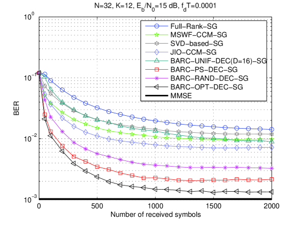
Figure 5: BER performance versus number of received symbols.

In order to assess the proposed decimation methods, we compute the BER performance of the algorithms for the uniform (U-DEC), the random (R-DEC), the prestored (PS-DEC) and the optimal (OPT-DEC) schemes. The results, shown in Fig. 5, indicate that the BARC scheme with the optimal decimation (OPT-DEC) achieves the best performance, followed by the proposed method with prestored decimation (PS-DEC), the random decimation system (R-DEC), the uniform decimation (U-DEC), the MSWF, the SVD and the full-rank approach. Due to its exponential complexity, the optimal decimation algorithm is not practical and the PS-DEC is the one with the best trade-off between performance and complexity.

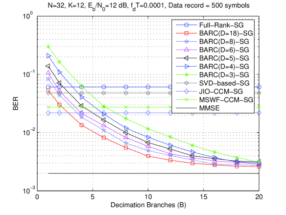
Figure 6: BER performance versus number of decimation branches.

In the next experiment, we evaluate the effect of the number of decimation branches $B$ on the performance for various ranks $D$ with a data support of $1500$ symbols and the PS-DEC decimation approach. The results, depicted in Fig. 6, indicate that the performance of the BARC scheme improves as $B$ is increased and approaches the optimal MMSE estimator, which assumes that the channels and the noise variance are known.

VI-C Performance with Model-Order Selection

In the next experiments, shown in Figs. 7 and 8, we assess the performance of the BARC scheme with the proposed model-order selection algorithm and mechanisms to determine the minimum number of branches necessary to attain a predefined performance as described in Section VI.

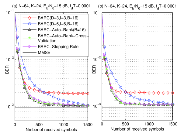
Figure 7: BER performance against number of symbols for different model-order selection algorithms with (a) SG and (b) RLS recursions.

The evaluation of the model-order selection algorithms is shown in Fig. 7, where we consider the BARC scheme with SG and RLS algorithms, $B=16$, $D_{\rm min}=3$, $D_{\rm max}=6$, and ${I_{\rm min}}=2$ and ${I_{\rm max}}=6$. We compare a configuration of the BARC scheme with $I=2$ and $D=3$, a second configuration of the BARC with $I=6$ and $D=6$, the BARC with the proposed model-order selection algorithm (Auto-Rank) with extended filters, the BARC with the method based on the stopping rule of [20] and the BARC with the CV-based algorithm of [21]. Notice that the BARC with the model-order selection algorithm based on multiple filters obtains a comparable performance to the Auto-Rank approach (the curves overlap and for this reason we do not shot it), however, the former is significantly more complex. The results indicate that the Auto-Rank allows the BARC scheme to achieve fast convergence and excellent steady state performance, which is close to the optimal MMSE. The performance of the Auto-Rank is slightly better than the stopping rule approach of [20] and the CV-based technique of [21]. The proposed Auto-Rank algorithm is less complex than the algorithms of [20] and [21] as it reduces the number of possible ranks to be used by the estimators by constraining them in a preselected range and does not require the computation of orthogonal projections as in [20].

In the next experiment, we assess the proposed SNB and SNB-S algorithms for automatically selecting the necessary number of branches to attain a predefined performance. The results are shown in Fig. 8 for an identical scenario to Fig. 7. We consider the BARC scheme with SG and RLS algorithms and the Auto-Rank algorithm for different values of $B$, and the proposed SNR and SNR-S algorithms. The parameter $\rho$ was set equal to $4\%$ greater than the MMSE and $B_{\rm{max}}=16$ for the experiment. The results indicate that the proposed branch adaptation techniques allow the BARC scheme to achieve a performance comparable to the BARC scheme with $B=16$. In particular, the proposed SNB algorithm achieves this performance with $B_{\rm{avg}}=7.6$, whereas the proposed SNB-S technique attains this performance with $B_{\rm{avg}}=5.4$ due to the use of a priori knowledge of the frequency of branch usage. In the following example, we consider the model-order selection and SNB-S algorithms for the BARC with the same parameters used in the previous experiment and the rank adaptation mechanisms proposed in [20] for the MSWF and in [21] for the AVF.

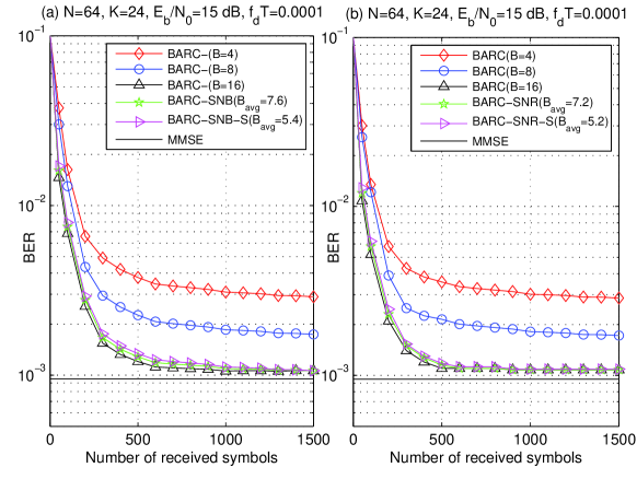
Figure 8: SINR performance against number of symbols with (a) SG and (b) RLS recursions.

VI-D Performance with Different Loads and SNR Values

In the last experiment, we assess the schemes and algorithms by computing the BER performance against $E_{b}/N_{0}$ and the number of users, as depicted in Fig. 9. The BER is evaluated for data records of $1500$ QPSK symbols and a scenario where the trained receivers employ pilot signals for estimating their parameters with SG and RLS algorithms, whereas the blind algorithms operate without any assistance. The maximum number of branches for the BARC scheme is $B_{\rm max}=16$ and we employed the proposed SNR-S algorithm.

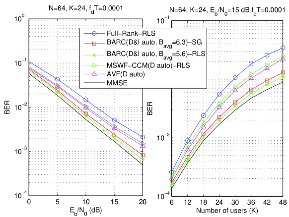
Figure 9: BER performance versus (a) $E_{b}/N_{0}$ (b) number of users for a data record of $500$ symbols.

The results show that the BARC scheme with both SG and RLS algorithms achieves a BER performance very close to the optimal MMSE, that assumes known channels, is followed by the AVF, the MSWF-RLS and the full-rank. Specifically, the BARC scheme with the SG algorithm can save up to $4$ dB in $E_{b}/N_{0}$ as compared to the AVF and the MSWF-RLS for the same BER and can accommodate up to $6$ more users as compared to the AVF and the MWF-RLS for the same BER.

VII Conclusions

This work proposes the BARC scheme and blind adaptive algorithms for interference suppression in wireless communications systems. The proposed BARC scheme employs a reduced-rank decomposition based on the concept of joint interpolation, switched decimation and reduced-rank estimation subject to a set of constraints. The proposed set of constraints ensures that the multi-path components of the channel are combined prior to dimensionality reduction. We have developed low-complexity SG and RLS reduced-rank estimation and model-order selection algorithms along with techniques for determining the required number of switching branches to attain a predefined performance. We have applied the proposed algorithms to interference suppression in DS-CDMA systems. The results of simulations indicate that the proposed BARC scheme allows a substantially better convergence and tracking performance than existing reduced-rank and full-rank schemes. This is due to the dimensionality reduction carried out by the proposed scheme that allows the use of adaptive algorithms with very small estimators. The proposed algorithms can be applied to other applications including MIMO systems, beamforming, broadband channel equalization and navigation systems.

Rodrigo C. de Lamare (S’99 - M’04 - SM’10) received the Diploma in electronic engineering from the Federal University of Rio de Janeiro (UFRJ) in 1998 and the M.Sc. and PhD degrees, both in electrical engineering, from the Pontifical Catholic University of Rio de Janeiro (PUC-Rio) in 2001 and 2004, respectively. Since January 2006, he has been with the Communications Research Group, Department of Electronics, University of York, where he is currently a lecturer in communications engineering. His research interests lie in communications and signal processing, areas in which he has published about 180 papers in refereed journals and conferences. Dr. de Lamare serves as associate editor for the EURASIP Journal on Wireless Communications and Networking. He is a Senior Member of the IEEE has served as the General Chair of the 7th IEEE International Symposium on Wireless Communications Systems, held in York, UK in September 2010.

Raimundo Sampaio-Neto received the Diploma and the M.Sc. degrees, both in electrical engineering, from Pontificia Universidade Católica do Rio de Janeiro (PUC-Rio) in 1975 and 1978, respectively, and the Ph.D. degree in electrical engineering from the University of Southern California (USC), Los Angeles, in 1983. From 1978 to 1979 he was an Assistant Professor at PUC-Rio, and from 1979 to 1983 he was a doctoral student and a Research Assistant in the Department of Electrical Engineering at USC with a fellowship from CAPES. From November 1983 to June 1984 he was a Post-Doctoral fellow at the Communication Sciences Institute of the Department of Electrical Engineering at USC, and a member of the technical staff of Axiomatic Corporation, Los Angeles. He is now a researcher at the Center for Studies in Telecommunications (CETUC) and an Associate Professor of the Department of Electrical Engineering of PUC-Rio, where he has been since July 1984. During 1991 he was a Visiting Professor in the Department of Electrical Engineering at USC. Prof. Sampaio has participated in various projects and has consulted for several private companies and government agencies. He was co-organizer of the Session on Recent Results for the IEEE Workshop on Information Theory, 1992, Salvador. He has also served as Technical Program co-Chairman for IEEE Global Telecommunications Conference (Globecom’99) held in Rio de Janeiro in December 1999 and as a member of the technical program committees of several national and international conferences. He was in office for two consecutive terms for the Board of Directors of the Brazilian Communications Society where he is now a member of its Advisory Council and Associate Editor of the Journal of the Brazilian Communication Society. His areas of interest include communication systems theory, digital transmission, satellite communications and signal processing for communications.

Martin Haardt (S’90 - M’98 - SM’99) has been a Full Professor in the Department of Electrical Engineering and Information Technology and Head of the Communications Research Laboratory at Ilmenau University of Technology, Germany, since 2001. After studying electrical engineering at the Ruhr-University Bochum, Germany, and at Purdue University, USA, he received his Diplom-Ingenieur (M.S.) degree from the Ruhr-University Bochum in 1991 and his Doktor-Ingenieur (Ph.D.) degree from Munich University of Technology in 1996. In 1997 he joined Siemens Mobile Networks in Munich, Germany, where he was responsible for strategic research for third generation mobile radio systems. From 1998 to 2001 he was the Director for International Projects and University Cooperations in the mobile infrastructure business of Siemens in Munich, where his work focused on mobile communications beyond the third generation. During his time at Siemens, he also taught in the international Master of Science in Communications Engineering program at Munich University of Technology. Martin Haardt has received the 2009 Best Paper Award from the IEEE Signal Processing Society, the Vodafone (formerly Mannesmann Mobilfunk) Innovations-Award for outstanding research in mobile communications, the ITG best paper award from the Association of Electrical Engineering, Electronics, and Information Technology (VDE), and the Rohde & Schwarz Outstanding Dissertation Award. In the fall of 2006 and the fall of 2007 he was a visiting professor at the University of Nice in Sophia-Antipolis, France, and at the University of York, UK, respectively. His research interests include wireless communications, array signal processing, high-resolution parameter estimation, as well as numerical linear and multi-linear algebra. Prof. Haardt has served as an Associate Editor for the IEEE Transactions on Signal Processing (2002-2006), the IEEE Signal Processing Letters (2006-2010), the Research Letters in Signal Processing (2007-2009), the Hindawi Journal of Electrical and Computer Engineering (since 2009), and as a guest editor for the EURASIP Journal on Wireless Communications and Networking. He has also served as the technical co-chair of the IEEE International Symposiums on Personal Indoor and Mobile Radio Communications (PIMRC) 2005 in Berlin, Germany, and as the technical program chair of the IEEE International Symposium on Wireless Communication Systems (ISWCS) 2010 in York, UK.

References

• [1]
• [2] M. L. Honig and H. V. Poor, โ€œAdaptive interference suppression,โ€ in Wireless Communications: Signal Processing Perspectives, H. V. Poor and G. W. Wornell, Eds. Englewood Cliffs, NJ: Prentice-Hall, 1998, Chapter 2, pp. 64-128.
• [3] S. Verdu, Multiuser Detection, Cambridge, 1998.
• [4] M. Honig and M. K. Tsatsanis, โ€œAdaptive techniques for multiuser CDMA receivers,โ€ IEEE Signal Processing Magazine, pp. 49-61,May 2000.
• [5] G. L. Stuber, J. R. Barry, S. W. MacLaughlin, Y. Li, M. A. Ingram and T. G. Pratt โ€Broadband MIMO-OFDM Wireless Communicationsโ€, Proceedings of the IEEE, vol. 92, no. 2, Feb 2004.
• [6] G. D. Golden, G. J. Foschini, R. A. Valenzuela, P. W. Wolniansky, โ€œDetection Algorithm and Initial Laboratory Results using the V-BLAST Space-Time Communication Architectureโ€, Electronics Letters, Vol. 35, No. 1, Jan. 7, 1999, pp. 14-15.
• [7] S. Haykin, Adaptive Filter Theory, 4th ed. Englewood Cliffs, NJ: Prentice- Hall, 2002.
• [8] J.C. Liberti and T. S. Rappaport, Smart Antennas for Wireless Communications: IS-95 and Third Generation CDMA Applications, Prentice Hall: Upper Saddle River, New Jersey, 1999.
• [9] M. Honig, U. Madhow and S. Verdu, โ€œBlind adaptive multiuser detection,โ€ IEEE Trans. Inf. Theory, vol. 41, pp. 944-960, July 1995.
• [10] Z. Xu and M.K. Tsatsanis, โ€œBlind adaptive algorithms for minimum variance CDMA receivers,โ€ IEEE Trans. Communications, vol. 49, No. 1, January 2001.
• [11] R. C. de Lamare and R. Sampaio-Neto, โ€œLow-Complexity Variable Step-Size Mechanisms for Stochastic Gradient Algorithms in Minimum Variance CDMA Receiversโ€, IEEE Trans. Signal Processing, vol. 54, pp. 2302 - 2317, June 2006.
• [12] C. Xu, G. Feng and K. S. Kwak, โ€œA Modified Constrained Constant Modulus Approach to Blind Adaptive Multiuser Detection,โ€ IEEE Trans. Communications, vol. 49, No. 9, 2001.
• [13] Z. Xu and P. Liu, โ€œCode-Constrained Blind Detection of CDMA Signals in Multipath Channels,โ€ IEEE Sig. Proc. Letters, vol. 9, No. 12, December 2002.
• [14] R. C. de Lamare and R. Sampaio Neto, โ€Blind Adaptive Code-Constrained Constant Modulus Algorithms for CDMA Interference Suppression in Multipath Channelsโ€, IEEE Communications Letters, vol 9. no. 4, April, 2005.
• [15] R. C. de Lamare, M. Haardt and R. Sampaio-Neto, โ€œBlind Adaptive Constrained Reduced-Rank Parameter Estimation based on Constant Modulus Design for CDMA Interference Suppression,โ€ IEEE Transactions on Signal Processing, vol. 56., no. 6, June 2008.
• [16] Y. Cai and R. C. de Lamare, โ€œLow-Complexity Variable Step Size Mechanism for Code-Constrained Constant Modulus Stochastic Gradient Algorithms applied to CDMA Interference Suppressionโ€, IEEE Transactions on Signal Processing, vol. 57, no. 1, January 2009.
• [17] R. C. de Lamare and R. Sampaio-Neto, โ€œBlind adaptive MIMO receivers for space-time block-coded DS-CDMA systems in multipath channels using the constant modulus criterion,โ€ IEEE Transactions on Communications, vol. 58, no. 1, January 2010, pp. 21-27.
• [18] L. L. Scharf and D. W. Tufts, โ€œRank reduction for modeling stationary signals,โ€ IEEE Trans. Acoust., Speech and Signal Processing, vol. ASSP-35, pp. 350-355, Mar. 1987.
• [19] X. Wang and H. V. Poor, โ€œBlind multiuser detection: A subspace approach,โ€ IEEE Trans. on Inf. Theory, vol. 44, pp. 677-690, March 1998.
• [20] M. L. Honig and J. S. Goldstein, โ€œAdaptive reduced-rank interference suppression based on the multistage Wiener filter,โ€ IEEE Trans. Commun., vol. 50, pp. 986-994, June 2002.
• [21] D. A. Pados, G. N. Karystinos, โ€œAn iterative algorithm for the computation of the MVDR filter,โ€ IEEE Trans. Sig. Proc., vol. 49, No. 2, February, 2001.
• [22] H. Qian and S. N Batalama, โ€œData record-based criteria for the selection of an auxiliary vector estimator of the MMSE/MVDR filterยดยด IEEE Trans. on Commun., vol. 51, No. 10, October 2003, pp. 1700-1708.
• [23] I. N. Psaromiligkos and S. N. Batalama, โ€Recursive short-datarecord estimation of AV and MMSE/MVDR linear filters for DS-CDMA antenna array systems,โ€ IEEE Transactions on Communications, vol. 52, pp.136-148, Jan. 2004.
• [24] L. Wang and R. C. de Lamare, โ€œAdaptive Constrained Constant Modulus Algorithm Based on Auxiliary Vector Filtering for Beamforming,โ€ IEEE Transactions on Signal Processing, vol.58, no.10, Oct. 2010, pp. 5410-5415.
• [25] R. C. de Lamare and Raimundo Sampaio-Neto, โ€œReduced-rank Interference Suppression for DS-CDMA based on Interpolated FIR Filtersโ€, IEEE Communications Letters, vol. 9, no. 3, March 2005.
• [26] R. C. de Lamare and R. Sampaio-Neto, โ€œAdaptive Reduced-Rank MMSE Filtering with Interpolated FIR Filters and Adaptive Interpolatorsโ€, IEEE Signal Processing Letters, vol. 12, no. 3, March, 2005.
• [27] R. C. de Lamare and R. Sampaio-Neto, โ€œAdaptive Interference Suppression for DS-CDMA Systems based on Interpolated FIR Filters with Adaptive Interpolators in Multipath Channelsโ€, IEEE Trans. Vehicular Technology, Vol. 56, no. 6, September 2007.
• [28] R. C. de Lamare and R. Sampaio-Neto, โ€œAdaptive Reduced-Rank MMSE Parameter Estimation based on an Adaptive Diversity Combined Decimation and Interpolation Scheme,โ€ Proc. IEEE International Conference on Acoustics, Speech and Signal Processing, April 15-20, 2007, vol. 3, pp. III-1317-III-1320.
• [29] R. C. de Lamare and R. Sampaio-Neto, โ€œReduced-Rank Adaptive Filtering Based on Joint Iterative Optimization of Adaptive Filtersโ€, IEEE Signal Processing Letters, Vol. 14, no. 12, December 2007.
• [30] R. C. de Lamare and R. Sampaio-Neto, โ€œReduced-Rank Space-Time Adaptive Interference Suppression With Joint Iterative Least Squares Algorithms for Spread-Spectrum Systems,โ€ IEEE Transactions on Vehicular Technology, vol.59, no.3, March 2010, pp.1217-1228.
• [31] R. C. de Lamare and R. Sampaio-Neto, โ€œAdaptive Reduced-Rank Processing Based on Joint and Iterative Interpolation, Decimation, and Filtering,โ€ IEEE Transactions on Signal Processing, vol. 57, no. 7, July 2009, pp. 2503 - 2514.
• [32] L. Wang, R. C. de Lamare, M. Yukawa, โ€œAdaptive Reduced-Rank Constrained Constant Modulus Algorithms Based on Joint Iterative Optimization of Filters for Beamforming,โ€ IEEE Transactions on Signal Processing, , vol. 58, no. 6, June 2010, pp. 2983-2997.
• [33] G. H. Golub and C. F. van Loan, Matrix Computations, 3rd ed., The Johns Hopkins University Press, Baltimore, Md, 1996.
• [34] D. Luenberger, Linear and Nonlinear Programming, 2nd Ed. Addison-Wesley, Inc., Reading, Massachusetts 1984.
• [35] C. T. Kelley, Iterative Methods for Optimization , no. 18 in Frontiers in Applied Mathematics, SIAM, Philadelphia, 1999.
• [36] T. S. Rappaport, Wireless Communications, Prentice-Hall, Englewood Cliffs, NJ, 1996.
• [37] D. Liberzon, Switching in Systems and Control, Birkhauser, 2003.
• [38] X. G. Doukopoulos and G. V. Moustakides, โ€œAdaptive Power Techniques for Blind Channel Estimation in CDMA Systemsโ€, IEEE Trans. Signal Processing, vol. 53, No. 3, March, 2005.
Rodrigo C. de Lamare (Sโ€™99 - Mโ€™04 - SMโ€™10) received the Diploma in electronic engineering from the Federal University of Rio de Janeiro (UFRJ) in 1998 and the M.Sc. and PhD degrees, both in electrical engineering, from the Pontifical Catholic University of Rio de Janeiro (PUC-Rio) in 2001 and 2004, respectively. Since January 2006, he has been with the Communications Research Group, Department of Electronics, University of York, where he is currently a lecturer in communications engineering. His research interests lie in communications and signal processing, areas in which he has published about 180 papers in refereed journals and conferences. Dr. de Lamare serves as associate editor for the EURASIP Journal on Wireless Communications and Networking. He is a Senior Member of the IEEE has served as the General Chair of the 7th IEEE International Symposium on Wireless Communications Systems, held in York, UK in September 2010.