Distributed adaptive steplength stochastic approximation schemes for Cartesian stochastic variational inequality problems

Abstract

Motivated by problems arising in decentralized control problems and non-cooperative Nash games, we consider a class of strongly monotone Cartesian variational inequality (VI) problems, where the mappings either contain expectations or their evaluations are corrupted by error. Such complications are captured under the umbrella of Cartesian stochastic variational inequality problems and we consider solving such problems via stochastic approximation (SA) schemes. Specifically, we propose a scheme wherein the steplength sequence is derived by a rule that depends on problem parameters such as monotonicity and Lipschitz constants. The proposed scheme is seen to produce sequences that are guaranteed to converge almost surely to the unique solution of the problem. To cope with networked multi-agent generalizations, we provide requirements under which independently chosen steplength rules still possess desirable almost-sure convergence properties. In the second part of this paper, we consider a regime where Lipschitz constants on the map are either unavailable or difficult to derive. Here, we present a local randomization technique that allows for deriving an approximation of the original mapping, which is then shown to be Lipschitz continuous with a prescribed constant. Using this technique, we introduce a locally randomized SA algorithm and provide almost sure convergence theory for the resulting sequence of iterates to an approximate solution of the original variational inequality problem. Finally, the paper concludes with some preliminary numerical results on a stochastic rate allocation problem and a stochastic Nash-Cournot game.

1 Introduction

Multi-agent system-theoretic problems can collectively capture a range of problems arising from decentralized control problems and noncooperative games. In static regimes, where agent problems are convex and agent feasibility sets are uncoupled, the associated solutions of such problems are given by the solution of a suitably defined Cartesian variational inequality problem. Our interest lies in settings where the mapping arising in such problems is strongly monotone and one of the following hold: (i) Either the mapping contains expectations whose analytical form is unavailable; or (ii) The evaluation of such a mapping is corrupted by error. In either case, the appropriate problem of interest is given by a stochastic variational inequality problem VI$(X,F)$ that requires determining an $x^{*}\in X$ such that

$$(x-x^{*})^{T}F(x^{*})\geq 0\qquad\hbox{for all }x\in X,$$ (1)

where

$$F(x)\triangleq\begin{pmatrix}\mathsf{E}\!\left[\Phi_{1}(x,\xi)\right]\\ \vdots\\ \mathsf{E}\!\left[\Phi_{N}(x,\xi)\right]\end{pmatrix},$$ (2)

$\Phi_{i}:{\cal D}_{i}\times\mathbb{R}^{d}\to\mathbb{R}^{n_{i}}$, ${\cal D}_{i}\subseteq\mathbb{R}^{n_{i}}$, $X$ is a closed and convex set, ${\cal D}_{i}$ is an open set in $\mathbb{R}^{n_{i}}$ and $\sum_{i=1}^{N}n_{i}=n$. Furthermore, $\xi:\Omega\to\mathbb{R}^{d}$ is a random variable, where $\Omega$ denotes the associated sample space and $\mathsf{E}\!\left[\cdot\right]$ denotes the expectation with respect to $\xi$.

Variational inequality problems assume relevance in capturing the solution sets of convex optimization and equilibrium problems [11]. Their Cartesian specializations arise from specifying the set $X$ as a Cartesian product, i.e., $X\triangleq\prod_{i=1}^{N}X_{i}$. Such problems arise in the modeling of multi-agent decision-making problems such as rate allocation problems in communication networks [18, 35, 31], noncooperative Nash games in communication networks [1, 2, 39], competitive interactions in cognitive radio networks [38, 30, 29, 20], and strategic behavior in power markets [17, 16, 32]. Our interest lies in regimes complicated by uncertainty, which could arise as a result of agents facing expectation-based objectives that do not have tractable analytical forms. Naturally, the Cartesian stochastic variational inequality problem framework represents an expansive model for capturing a range of such problems.

Two broad avenues exist for solving such a class of problems. Of these, the first approach, referred to as the sample-average approximation (SAA) method. In adopting this approach, one uses a set of $M$ samples $\{\xi_{1},\ldots,\xi_{M}\}$ and considers the sample-average problem where an expected mapping $\mathsf{E}\!\left[\Phi(x,\xi)\right]$ is replaced by the sample-average ${\sum_{j=1}^{M}\Phi(x,\xi^{j})}/{M}$. The resulting problem is deterministic and its solution provides an estimator for the solution of the true problem. The asymptotic behavior of these estimators has been studied extensively in the context of stochastic optimization and variational problems [23, 33]. The other approach, referred to as stochastic approximation, also has a long tradition. First proposed by Robbins and Monro [28] for root-finding problems and by Ermoliev for stochastic programs [8, 10, 9], significant effort has been applied towards theoretical and algorithmic examination of such schemes (cf. [4, 21, 34]). Yet, there has been markedly little on the application of such techniques to solution of stochastic variational inequalities, exceptions being [14, 19]. Standard stochastic approximation schemes provide little guidance regarding the choice of a steplength sequence, denoted by $\{\gamma_{k}\}$, apart from requiring that the sequence satisfies

$$\sum_{k=0}^{\infty}\gamma_{k}=\infty\quad\mbox{ and }\quad\sum_{k=0}^{\infty}\gamma_{k}^{2}<\infty.$$

The behavior of stochastic approximation schemes is closely tied to the choice of steplength sequences. Generally, there have been two avenues traversed in choosing steplengths: (i) Deterministic steplength sequences: Spall [34, Ch. 4, pg. 113] considered diverse choices of the form $\gamma_{k}=\frac{\beta}{(k+1+a)^{\alpha}}$, where $\beta>0$, $0<\alpha\leq 1$, and $a\geq 0$ is a stability constant. In related work in the context of approximate dynamic programming, Powell [27] examined several deterministic update rules. However, much of these results are not provided with convergence theory. (ii) Stochastic steplength sequences: An alternative to a deterministic rule is a stochastic scheme that updates steplengths based on observed data. Of note is recent work by George et al. [12] where an adaptive stepsize rule is proposed that minimizes the mean squared error. In a similar vein, Cicek et al. [7] develop an adaptive Kiefer-Wolfowitz SA algorithm and derive general upper bounds on its mean-squared error.

Before proceeding, we note the relationship of the present work to three specific references. In  [19], Cartesian stochastic variational inequality problems with Lipschitzian mappings were considered with a focus towards integrating Tikhonov and prox-based regularization techniques with standard stochastic gradient methods. However, the steplength sequences were “non-adaptive” since the choices did not adapt to problem parameters. Two problem-specific adaptive rules were developed in our earlier work on stochastic convex programming. Additionally, local smoothing techniques were examined for addressing the lack of smoothness. Of these, the first, referred to as the recursive steplength SA scheme, forms the inspiration for a generalization pursued in the current work. Finally, in [40], we extended this recursive rule to accommodate stochastic variational inequality problems. Note that the qualifier “adaptive” implies that the steplength rule adapts to problem parameters such as Lipschitz constant, monotonicity constant and the diameter of the set. In this paper, our goal lies in developing a distributed adaptive stochastic approximation scheme (DASA) that can accommodate networked multi-agent implementations and cope with non-Lipschitzian mappings. More specifically, the main contributions of this paper are as follows:

(i) DASA schemes for Lipschitzian CSVIs:

We begin with a simple extension of the adaptive stepength rule presented in [41] to the variational regime under a Lipschitzian requirement on the map. Yet, implementing this rule in a centralized regime is challenging and this motivates the need for distributed counterparts that can be employed on Cartesian problems. Such a distributed rule is developed and produces sequences of iterates that are guaranteed to converge to the solution in almost-sure sense.

(ii) DASA schemes for non-Lipschitzian CSVIs:

Our second goal lies in addressing the absence or unavailability of a Lipschitz constant by leveraging locally randomized smoothing techniques, again inspired by our efforts to solve nonsmooth stochastic optimization problems [41]. In this part of the paper, we generalize this natively centralized scheme for optimization problems to a distributed version that can cope with Cartesian stochastic variational inequality problems.

The remainder of this paper is organized as follows. In Section 2, we provide a canonical formulation for the problem of interest and motivate this formulation through two sets of examples. An adaptive steplength SA scheme for stochastic variational inequality problems with Lipschitzian mappings and its distributed generalization are provided in Section 3. By leveraging a locally randomized smoothing technique, in Section 4, we extend these schemes to a regime where Lipschitzian assumptions do not hold. Finally, the paper concludes with some preliminary numerics in Section 5.

Notation: Throughout this paper, a vector $x$ is assumed to be a column vector. We write $x^{T}$ to denote the transpose of a vector $x$, $\|x\|$ to denote the Euclidean vector norm, i.e., $\|x\|=\sqrt{x^{T}x}$, $\|x\|_{1}$ to denote the $1$-norm, i.e., $\|x\|_{1}=\sum_{i=1}^{n}|x_{i}|$ for $x\in\mathbb{R}^{n}$, and $\|x\|_{\infty}$ to denote the infinity vector norm, i.e., $\|x\|_{\infty}=\max_{i=1,\ldots,n}|x_{i}|$ for $x\in\mathbb{R}^{n}$. We use $\Pi_{X}(x)$ to denote the Euclidean projection of a vector $x$ on a set $X$, i.e., $\|x-\Pi_{X}(x)\|=\min_{y\in X}\|x-y\|$. For a convex function $f$ with domain dom$f$, a vector $g$ is a subgradient of $\bar{x}\in\hbox{dom}f$ if $f(\bar{x})+g^{T}(x-\bar{x})\leq f(x)$ holds for all $x\in\hbox{dom}f.$ The set of all subgradients of $f$ at $\bar{x}$ is denoted by $\partial f(\bar{x})$. We write a.s. as the abbreviation for “almost surely”. We use $\mathsf{Prob}(A)$ to denote the probability of an event $A$ and $\mathsf{E}\!\left[z\right]$ to denote the expectation of a random variable $z$. The Matlab notation $(u_{1};u_{2};u_{3})$ refers to a column vector with components $u_{1}$, $u_{2}$ and $u_{3}$, respectively.

2 Formulation and source problems

In Section 2.1, we formulate the Cartesian stochastic variational inequality (CSVI) problem and outline the stochastic approximation algorithmic framework. A motivation for studying CSVIs is provided through two examples in Section 2.2, while a review of the main assumptions is given in Section 2.3.

2.1 Problem formulation and algorithm outline

Given a set $X\subseteq\mathbb{R}^{n}$ and a mapping $F:X\to\mathbb{R}^{n}$, the variational inequality problem, denoted by VI$(X,F)$, requires determining a vector $x^{*}\in X$ such that $(x-x^{*})^{T}F(x^{*})\geq 0$ holds for all $x\in X$. When the underlying set $X$ is given by a Cartesian product, as articulated by the definition $X\triangleq\prod_{i=1}^{N}X_{i}$, where $X_{i}\subseteq\mathbb{R}^{n_{i}}$, then the associated variational inequality is qualified as a Cartesian variational inequality problem. Now suppose that ${x^{*}=(x_{1}^{*};x_{2}^{*};\ldots;x_{N}^{*})}\in X$ satisfies the following system of inequalities:

$$(x_{i}-x_{i}^{*})^{T}\mathsf{E}\!\left[\Phi_{i}(x^{*},\xi_{i})\right]\geq 0\qquad\hbox{ for all $x_{i}\in X_{i}$ and all $i=1,\ldots,N$},$$ (3)

where $\xi_{i}:{\Omega_{i}}\rightarrow R^{d_{i}}$ is a random vector with some probability distribution for $i=1,\ldots,N$. Naturally, problem (3) may be reduced to VI$(X,F)$ by noting that $F$ may be defined as in (2), where $n=\sum_{i=1}^{N}n_{i}$ and $F:X\to\mathbb{R}^{n}$. Then, VI$(X,F)$ is a stochastic variational inequality problem on the Cartesian product of the sets $X_{i}$ with a solution $x^{*}=(x_{1}^{*};x_{2}^{*};\ldots;x_{N}^{*})$.

Much of the interest in this paper pertains to the development of stochastic approximation schemes for VI$(X,F)$ when the components the map $F$ is defined by (2). For such a problem, we consider the following distributed stochastic approximation scheme:

$$\begin{aligned} x_{{k+1},i}&=\Pi_{X_{i}}\left(x_{k,i}-\gamma_{k,i}(F_{i}(x_{k})+w_{k,i})\right),\cr w_{k,i}&\triangleq{{\color[rgb]{0,0,0}\Phi_{i}(x_{k}}},\xi_{k,i})-F_{i}(x_{k}),\end{aligned}$$ (4)

for all $k\geq 0$ and $i=1,\dots,N$, where $F_{i}(x)\triangleq\mathsf{E}\!\left[\Phi_{i}(x,\xi_{i})\right]$ for $i=1,\ldots,N$, $\gamma_{k,i}>0$ is the stepsize for the $i$th index at iteration $k$, $x_{k,i}$ denotes the solution for the $i$-th index at iteration $k$, and $x_{k}=(x_{k,1};\ x_{k,2};\ \ldots;\ x_{k,N})$. Moreover, $x_{0}\in X$ is a random initial vector independent of any other random variables in the scheme and such that $\mathsf{E}\!\left[\|x_{0}\|^{2}\right]<\infty$.

2.2 Motivating examples

We consider two problems that can be addressed by Cartesian stochastic variational inequality framework.

Example 1 (Networked stochastic Nash-Cournot game).

A classical example of a Nash game is a networked Nash-Cournot game [24, 15]. Suppose a collection of $N$ firms compete over a network of $M$ nodes wherein the production and sales for firm $i$ at node $j$ are denoted by $g_{ij}$ and $s_{ij}$, respectively. Suppose firm $i$’s cost of production at node $j$ is denoted by the uncertain cost function $c_{ij}(g_{ij},\xi)$. Furthermore, goods sold by firm $i$ at node $j$ fetch a random revenue defined by $p_{j}(\bar{s}_{j},\xi)s_{ij}$ where $p_{j}(\bar{s}_{j},\xi)$ denotes the uncertain sales price at node $j$ and $\bar{s}_{j}=\sum_{i=1}^{N}s_{ij}$ denotes the aggregate sales at node $j$. Finally, firm $i$’s production at node $j$ is capacitated by $\mathrm{cap}_{ij}$ and its optimization problem is given by the following:

minimize $$\qquad{\mathsf{E}\!\left[f_{i}(x,\xi)\right]}$$

subject to $$\qquad x_{i}\in X_{i},$$

where $x=(x_{1};\ldots;x_{N})$ with $x_{i}=(g_{i};s_{i})$, $g_{i}=(g_{i1};\ldots;g_{iM})$, $s_{i}=(s_{i1};\ldots;s_{iM})$, and

$$f_{i}(x,\xi) \triangleq\sum_{j=1}^{M}\left(c_{ij}(g_{ij},\xi)-p_{j}(\bar{s}_{j},\xi)s_{ij}\right),$$

$$X_{i} \triangleq\left\{(g_{i},s_{i})\mid\sum_{j=1}^{M}g_{ij}=\sum_{j=1}^{M}s_{ij},\quad g_{ij},\,s_{ij}\geq 0,\quad g_{ij}\leq\mathrm{cap}_{ij},\ j=1,\ldots,M\right\}.\hfill\qed$$

Under the validity of the interchange between the expectation and the derivative operator, the resulting equilibrium conditions of this stochastic Nash-Cournot game are compactly captured by the variational inequality VI$(X,F)$ where $X\triangleq\prod_{i=1}^{N}X_{i}$ and $F(x)=(F_{1}(x);\ldots;F_{N}(x))$ with $F_{i}(x)=\mathsf{E}\!\left[\nabla_{x_{i}}f_{i}(x,\xi)\right]$.

Example 2 (Stochastic composite minimization problem).

Consider a generalized min-max optimization problem given by

minimize $$\qquad\Psi(\psi_{1}(x),\ldots,\psi_{m}(x))$$ (5)

subject to $$\qquad x\in X\triangleq\prod_{i=1}^{N}X_{i},$$ (6)

where $\Psi(u_{1},\ldots,u_{m})$ is defined as

$$\Psi(u_{1},\ldots,u_{m})\triangleq\max_{y\in{\mathcal{Y}}}\left\{\sum_{i=1}^{m}u_{i}^{T}(A_{i}y+b_{i})-\beta(y)\right\},$$

while ${\psi_{i}(x)}\triangleq\mathsf{E}\!\left[{\phi_{i}}(x,\xi)\right]$, $\nabla_{x_{j}}\psi_{i}(x)=\mathsf{E}\!\left[H_{ji}(x,\xi)\right]$ for $i=1,\ldots,m,$ and ${\beta(y)}$ is a Lipschitz continuous convex function of $y$. ∎

Under the assumption that the derivative and the expectation operator can be interchanged, it can be seen that the solution to this optimization problem can be obtained by solving a Cartesian stochastic variational inequality problem VI$(X\times{\mathcal{Y}},F)$ where

$$F(x,y)\triangleq\displaystyle\begin{pmatrix}\sum_{i=1}^{m}\nabla_{x_{1}}{\psi_{i}(x)}(A_{i}y+b_{i})\\ \vdots\\ \sum_{i=1}^{m}\nabla_{x_{N}}{\psi_{i}(x)}(A_{i}y+b_{i})\\ -\sum_{i=1}^{m}A_{i}^{T}\psi_{i}(x)+\nabla_{y}\beta(y)\end{pmatrix}=\begin{pmatrix}\mathsf{E}\left[\sum_{i=1}^{m}H_{1i}(x,\xi)(A_{i}y+b_{i})\right]\\ \vdots\\ \mathsf{E}\left[\sum_{i=1}^{m}H_{Ni}(x,\xi)(A_{i}y+b_{i})\right]\\ \mathsf{E}\left[-\sum_{i=1}^{m}A_{i}^{T}\phi_{i}(x,\xi)+\nabla_{y}\beta(y)\right]\end{pmatrix}.$$

Note that the specification that ${\psi_{i}(x)}$ and its Jacobian are expectation-valued may be a consequence of not having access to noise-free evaluations of either object. In particular, one only has access to evaluations $\phi_{i}(x,\xi)$ and Jacobian evaluations given by $H_{ji}(x,\xi)=\nabla_{x_{j}}{\phi_{i}(x,\xi)}$.

2.3 Assumptions

Our interest lies in the development of distributed stochastic approximation schemes for Cartesian stochastic variational inequality problems as espoused by (4) and the associated global convergence theory in regimes where the mappings are single-valued mappings that are not necessarily Lipschitz continuous. We let

$$X=\prod_{i=1}^{N}X_{i},$$

and make the following assumptions on the set $X$ and the mapping $F$.

Assumption 1.

Assume the following:

1. The set $X_{i}\subseteq\mathbb{R}^{n_{i}}$ is closed and convex for $i=1,\ldots,N$.

2. The mapping $F(x)$ is a single-valued Lipschitz continuous over the set $X$ with a constant $L$.

3. The mapping $F(x)$ is strongly monotone with a constant $\eta>0$:

   $$(F(x)-F(y))^{T}(x-y)\geq\eta\|x-y\|^{2}\qquad\hbox{for all }x,y\in{X}.$$

Since $F$ is strongly monotone, the existence and uniqueness of the solution to VI$(X,F)$ is guaranteed by Theorem 2.3.3 of [11]. We let $x^{*}$ denote the solution of VI$(X,F)$.

Regarding the method in (4), we let $\mathcal{F}_{k}$ denote the history of the method up to time $k$, i.e., $\mathcal{F}_{k}=\{x_{0},\xi_{0},\xi_{1},\ldots,\xi_{k-1}\}$ for $k\geq 1$ and $\mathcal{F}_{0}=\{x_{0}\}$, where $\xi_{k}=(\xi_{k,1}\ ;\xi_{k,2}\ ;\ldots\ ;\xi_{k,N})$. In terms of this definition, we note that

$$\mathsf{E}\!\left[w_{k,i}\mid\mathcal{F}_{k}\right]=\mathsf{E}\!\left[{{\color[rgb]{0,0,0}\Phi_{i}(x_{k}}},\xi_{k,i})\mid\mathcal{F}_{k}\right]-F_{i}(x_{k})=0\qquad\hbox{for all $k\geq 0$ and all $i$}.$$

We impose some further conditions on the stochastic errors $w_{k,i}$ of the algorithm, as follows.

Assumption 2.

The errors $w_{k}=(w_{k,1};w_{k,2};\ldots;w_{k,N})$ are such that for some (deterministic) $\nu>0$,

$$\mathsf{E}\!\left[\|w_{k}\|^{2}\mid\mathcal{F}_{k}\right]\leq\nu^{2}\qquad\hbox{{a.s.} for all $k\geq 0$}.$$

We use the following Lemma in establishing the convergence of method (4) and its extensions. This result may be found in [26] (cf. Lemma 10, page 49).

Lemma 1.

Let $\{v_{k}\}$ be a sequence of nonnegative random variables, where $\mathsf{E}\!\left[v_{0}\right]<\infty$, and let $\{\alpha_{k}\}$ and $\{\mu_{k}\}$ be deterministic scalar sequences such that:

$$\mathsf{E}\!\left[v_{k+1}|v_{0},\ldots,v_{k}\right]\leq(1-\alpha_{k})v_{k}+\mu_{k}\qquad a.s.\ \hbox{for all }k\geq 0,$$

$$0\leq\alpha_{k}\leq 1,\quad\ \mu_{k}\geq 0,\qquad\hbox{for all }k\geq 0,$$

$$\sum_{k=0}^{\infty}\alpha_{k}=\infty,\quad\ \sum_{k=0}^{\infty}\mu_{k}<\infty,\quad\ \lim_{k\to\infty}\,\frac{\mu_{k}}{\alpha_{k}}=0.$$

Then, $v_{k}\rightarrow 0$ almost surely, $\lim_{k\to\infty}\mathsf{E}\!\left[v_{k}\right]=0$, and for any $\epsilon>0$ and for all $k>0$,

$$\mathsf{Prob}\left(\{v_{j}\leq\epsilon\hbox{ for all }j\geq k\}\right)\geq 1-\frac{1}{\epsilon}\left(\mathsf{E}\!\left[v_{k}\right]+\sum_{i=k}^{\infty}\beta_{i}\right).$$

3 Distributed adaptive SA schemes for Lipschitzian mappings

In this section, we restrict our attention to settings where the mapping $F(x)$ is a single-valued Lipschitzian map. In Section 3.1, we begin by developing an adaptive steplength rule for deriving steplength sequences from problem parameters such as monotonicity constant, Lipschitz constant etc., where the qualifier adaptive implies that the steplength choices “adapt” or are “self-tuned” to problem parameters. Unfortunately, in distributed regimes, such a rule requires prescription by a central coordinator, a relatively challenging task in multi-agent regimes. This motivates the development of a distributed counterpart of the aforementioned adaptive rule and provide convergence theory for such a generalization in Section 3.2.

3.1 An adaptive steplength SA (ASA) scheme

Stochastic approximation algorithms require stepsize sequences to be square summable but not summable. These algorithms provide little advice regarding the choice of such sequences. One of the most common choices has been the harmonic steplength rule which takes the form of $\gamma_{k}=\frac{\theta}{k}$ where $\theta>0$ is a constant. Although, this choice guarantees almost-sure convergence, it does not leverage problem parameters. Numerically, it has been observed that such choices can perform quite poorly in practice. Motivated by this shortcoming, we present a steplength scheme for a centralized variant of algorithm (4):

$$\begin{aligned} x_{{k+1}}&=\Pi_{X}\left(x_{k}-\gamma_{k}(F(x_{k})+w_{k})\right),\cr w_{k}&\triangleq{{\color[rgb]{0,0,0}\Phi(x_{k}}},\xi_{k})-F(x_{k}),\end{aligned}$$ (7)

for $k\geq 0$. The proposed scheme derives a rule for updating steplength sequences that adapts to problem parameters while guaranteeing almost-sure convergence of $x_{k}$ to the unique solution of VI$(X,F)$.

A key challenge in practical implementations of stochastic approximation lies in choosing an appropriate diminishing steplength sequence $\{\gamma_{k}\}$. In [41], we developed a rule for selecting such a sequence in a convex stochastic optimization regime by leveraging three parameters: (i) Lipschitz constant of the gradients; (ii) strong convexity constant; and (ii) diameter of the set $X$. Along similar directions, such a rule is constructed for strongly monotone stochastic variational inequality problems and the results in this subsection bear significant similarity to those presented in [41] with some key distinctions. First, these results are presented for strongly monotone stochastic variational inequality problems and second, co-coercivity of the mappings is not assumed, leading to a tighter requirement on the choice of steplengths.

Lemma 2.

Consider algorithm (7), and let Assumptions 1 and 2 hold. Then, the following relation holds almost surely for all $k\geq 0$:

$$\mathsf{E}\!\left[\|x_{k+1}-x^{*}\|^{2}\mid\mathcal{F}_{k}\right]\leq(1-2\eta\gamma_{k}+L^{2}\gamma_{k}^{2})\|x_{k}-x^{*}\|^{2}+{\gamma_{k}^{2}\nu^{2}}.$$ (8)

Proof.

By the definition of algorithm (7) and the non-expansiveness property of the projection operator, we have for all $k\geq 0$,

$$\|x_{k+1}-x^{*}\|^{2} =\|\Pi_{X}(x_{k}-\gamma_{k}(F(x_{k})+w_{k}))-\Pi_{X}(x^{*}-\gamma_{k}F(x^{*}))\|^{2}$$

$$\leq\|x_{k}-x^{*}-\gamma_{k}(F(x_{k})+w_{k}-F(x^{*}))\|^{2}.$$

Taking expectations conditioned on the past, and by employing $\mathsf{E}\!\left[w_{k}\mid\mathcal{F}_{k}\right]=0$, we have

$$\mathsf{E}\!\left[\|x_{k+1}-x^{*}\|^{2}\mid\mathcal{F}_{k}\right] \leq\|x_{k}-x^{*}\|^{2}+\gamma_{k}^{2}\|F(x_{k})-F(x^{*})\|^{2}+\gamma_{k}^{2}\mathsf{E}\!\left[\|w_{k}\|^{2}\mid\mathcal{F}_{k}\right]$$

$$-2\gamma_{k}(x_{k}-x^{*})^{T}(F(x_{k})-F(x^{*}))$$

$$\leq(1-2\eta\gamma_{k}+\gamma_{k}^{2}L^{2})\|x_{k}-x^{*}\|^{2}+\gamma_{k}^{2}\nu^{2},$$

where the second inequality is a consequence of the strong monotonicity and Lipschitz continuity of $F(x)$ over $X$ as well as the boundedness of $\mathsf{E}\!\left[\|w_{k}\|^{2}\mid\mathcal{F}_{k}\right].$ ∎

The upper bound (8) can be used to construct an adaptive stepsize rule. Note that inequality (8) holds for any $\gamma_{k}>0$. When the stepsize is further restricted so that $0<\gamma_{k}\leq\frac{\eta}{L^{2}}$, we have

$$1-\gamma_{k}(2\eta-\gamma_{k}L^{2})\leq 1-\eta\gamma_{k}.$$

Thus, for $0<\gamma_{k}\leq\frac{\eta}{L^{2}}$ and by taking expectations, inequality (8) reduces to

$$\mathsf{E}\!\left[\|x_{k+1}-x^{*}\|^{2}\right]\leq(1-\eta\gamma_{k})\mathsf{E}\!\left[\|x_{k}-x^{*}\|^{2}\right]+\gamma_{k}^{2}\nu^{2}\qquad\hbox{for all }k\geq 0.$$ (9)

We begin by viewing $\mathsf{E}\!\left[\|x_{k+1}-x^{*}\|^{2}\right]$ as an error $e_{k+1}$ arising from employing the stepsize sequence $\gamma_{0},\gamma_{1},\ldots,\gamma_{k}$. Furthermore, the worst case error arises when (9) holds as an equality and satisfies the following recursive relation:

$$e_{k+1}(\gamma_{0},\ldots,\gamma_{k})=(1-\eta\gamma_{k})e_{k}(\gamma_{0},\ldots,\gamma_{k-1})+\gamma_{k}^{2}\nu^{2}.$$

Motivated by this relationship, our interest lies in examining whether the stepsizes $\gamma_{0},\gamma_{1}\ldots,\gamma_{k}$ can be chosen so as to minimize the error $e_{k}$. Our goal lies in constructing a stepsize scheme that allows for claiming the almost sure convergence of the sequence $\{x_{k}\}$ produced by algorithm (7) to the unique solution $x^{*}$ of VI$(X,F)$. We formalize this approach by defining real-valued error functions $e_{k}(\gamma_{0},\ldots,\gamma_{k-1})$ as follows:

$$e_{k}(\gamma_{0},\ldots,\gamma_{k-1}) \triangleq(1-\eta\gamma_{k-1})e_{k-1}(\gamma_{0},\ldots,\gamma_{k-2})+\gamma_{k-1}^{2}\nu^{2}\qquad\hbox{for $k\geq 1$},$$ (10)

where $e_{0}$ is a positive scalar, $\eta$ is the strong monotonicity constant and $\nu^{2}$ is an upper bound for the second moments of the error norms $\|w_{k}\|$. We consider a choice of $\{\gamma_{0},\gamma_{1},\ldots,\gamma_{k-1}\}$ based on minimizing an upper bound on the mean-squared error, namely $e(\gamma_{0},\gamma_{1},\ldots,\gamma_{k-1})$, as captured by the following optimization problem:

$$\begin{split}&\begin{array}[]{ll}\hbox{minimize }&e_{k}(\gamma_{0},\ldots,\gamma_{k-1})\cr\hbox{subject to }&0<\gamma_{j}\leq\frac{\eta}{L^{2}}\hbox{ for all }j=0,\ldots,k-1.\end{array}\end{split}$$

To ensure convergence in an almost-sure sense, the sequence $\{\gamma_{k}\}$ needs to satisfy $\sum_{j=0}^{\infty}\gamma_{j}=\infty$ and $\sum_{j=0}^{\infty}\gamma_{j}^{2}<\infty$. As the next two propositions show, these can indeed be achieved. In fact, the error $e_{k+1}$ at the next iteration can also be minimized by selecting $\gamma_{k}$ as a function of only the most recent stepsize $\gamma_{k-1}$. In what follows, we consider the sequence $\{\gamma^{*}_{k}\}$ given by

$$\gamma_{0}^{*}=\frac{\eta}{2\nu^{2}}\,e_{0}$$ (11)

$$\gamma_{k}^{*}=\gamma_{k-1}^{*}\left(1-\frac{\eta}{2}\gamma_{k-1}^{*}\right)\quad\hbox{for all }k\geq 1.$$ (12)

We provide a result showing that the stepsizes $\gamma_{i}$, $i=0,\ldots,k-1,$ minimize $e_{k}$ over $(0,\frac{\eta}{L^{2}}]^{k}$, where $L$ is the Lipschitz constant associated with $F(x)$ over $X$.

Proposition 1 (An adaptive steplength SA (ASA) scheme).

Let the error function $e_{k}(\gamma_{0},\ldots,\gamma_{k-1})$ be defined as in (10), where $e_{0}\geq 0$ is such that $\nu\geq L\,\sqrt{\frac{e_{0}}{2}}$, where $L$ is the Lipschitz constant of $F$. Let the sequence $\{\gamma^{*}_{k}\}$ be given by (11)–(12). Then, the following hold:

• For all $k\geq 0$, the error $e_{k}$ satisfies $e_{k}(\gamma_{0}^{*},\ldots,\gamma_{k-1}^{*})=\frac{2\nu^{2}}{\eta}\,\gamma_{k}^{*}$.

• For each $k\geq 1$, the vector $(\gamma_{0}^{*},\gamma_{1}^{*},\ldots,\gamma_{k-1}^{*})$ is the minimizer of the function $e_{k}(\gamma_{0},\ldots,\gamma_{k-1})$ over the set

  $$\mathbb{G}_{k}\triangleq\left\{\alpha\in\mathbb{R}^{k}:0<\alpha_{j}\leq\frac{\eta}{L^{2}}\hbox{ for }j=1,\ldots,k\right\}.$$

  More precisely, for any $k\geq 1$ and any $(\gamma_{0},\ldots,\gamma_{k-1})\in\mathbb{G}_{k}$, we have

  $$e_{k}(\gamma_{0},\ldots,\gamma_{k-1})-e_{k}(\gamma_{0}^{*},\ldots,\gamma_{k-1}^{*})\geq\nu^{2}(\gamma_{k-1}-\gamma_{k-1}^{*})^{2}.$$

The almost-sure convergence of the produced sequence holds for a family of steplength rules, as captured by the folloing result.

Proposition 2 (Almost-sure convergence of ASA scheme).

Let Assumptions 1 and 2 hold. Assume that the stepsize sequence $\{\gamma_{k}\}$ is generated by the following adaptive scheme:

$$\gamma_{k}=\gamma_{k-1}(1-c\gamma_{k-1})\qquad\hbox{for all }k\geq 1,$$

where $c>0$ is a scalar and the initial stepsize is such that $0<\gamma_{0}<\frac{1}{c}$. Then, the sequence $\{x_{k}\}$ generated by algorithm (7) converges almost surely to a random point that belongs to the optimal set.

The proofs of Propositions 1 and 2 are omitted, as they follow from a more general results for a distributed SA method, as discussed in the next subsection.

3.2 A distributed adaptive steplength SA (DASA) scheme

Unfortunately, in multi-agent regimes, the implementation of the stepsize rule (11)-(12) requires a central coordinator who can prescribe and enforce such rules. In this section, we extend the centralized rule to accommodate a multi-agent setting wherein each agent chooses its own update rule, given the global knowledge of problem parameters. In such a regime, given that the set $X$ is the Cartesian product of closed and convex sets $X_{1},\ldots,X_{N}$, our interest lies in developing steplength update rules in the context of method (4) where the $i$-th agent chooses its steplength, denoted by $\gamma_{k,i}$, as per

$$\gamma_{k,i}=\gamma_{k-1,i}(1-c_{i}\gamma_{k-1,i}),$$

with $c_{i}>0$ being a constant associated with agent $i$ mapping $F_{i}(x)$, while the initial stepsize $\gamma_{0,i}$ is suitably selected. The following assumption imposes requirements on the stepsizes $\gamma_{k,i}$ in (4).

Assumption 3.

Assume that the following hold:

1. The stepsize sequences $\{\gamma_{k,i}\}$, $i=1,\ldots,N$, are such that $\gamma_{k,i}>0$ for all $k$ and $i$, with $\sum_{k=0}^{\infty}\gamma_{k,i}=\infty$ and $\sum_{k=0}^{\infty}\gamma_{k,i}^{2}<\infty$ for all $i$.

2. If $\{\delta_{k}\}$ and $\{\Gamma_{k}\}$ are positive sequences such that $\delta_{k}\leq\min_{1\leq i\leq N}{\gamma_{k,i}}$ and $\Gamma_{k}\geq\max_{1\leq i\leq N}{\gamma_{k,i}}$ for all $k\geq 0$, then

   $$\frac{\Gamma_{k}-\delta_{k}}{\delta_{k}}\leq\beta\qquad\hbox{for all $k\geq 0$},$$

   where $\beta$ is a scalar satisfying $0\leq\beta<\frac{\eta}{L}$.

Remark: Assumption  (3a) is a standard requirement on steplength sequences while Assumption (3b) provides an additional condition on the discrepancy between the stepsize values $\gamma_{k,i}$ at each iteration $k$. This condition is satisfied, for instance, when $\gamma_{k,1}=\ldots=\gamma_{k,N}$, in which case $\beta=0$.

When deriving an adaptive rule, we use Lemma 1 and a distributed generalization of Lemma 2, which is given below.

Lemma 3.

Consider algorithm (4). Let Assumptions 1 and 2 hold.

1. The following relation holds almost surely for all $k\geq 0$:

   $$\mathsf{E}\!\left[\|x_{k+1}-x^{*}\|^{2}\mid\mathcal{F}_{k}\right]\leq(1-2(\eta+L)\delta_{k}+2L\Gamma_{k}+L^{2}\Gamma_{k}^{2})\|x_{k}-x^{*}\|^{2}+{{\color[rgb]{0,0,0}\Gamma_{k}^{2}\nu^{2}}},$$

   where $\{\delta_{k}\}$ and $\{\Gamma_{k}\}$ are positive sequences such that $\delta_{k}\leq\min_{1\leq i\leq N}{\gamma_{k,i}}$ and $\Gamma_{k}\geq\max_{1\leq i\leq N}{\gamma_{k,i}}$ for all $k$.

2. If Assumption (3b) holds, then the following relation is valid for all $k\geq 0$:

   $$\mathsf{E}\!\left[\|x_{k+1}-x^{*}\|^{2}\right]\leq(1-2(\eta-\beta L)\delta_{k}+(1+\beta)^{2}L^{2}\delta_{k}^{2})\mathsf{E}\!\left[\|x_{k}-x^{*}\|^{2}\right]+(1+\beta)^{2}\delta_{k}^{2}\nu^{2}.$$

Proof.

(a) From the properties of the projection operator, we know that a vector $x^{*}$ solves VI$(X,F)$ problem if and only if $x^{*}$ satisfies $x^{*}=\Pi_{X}(x^{*}-\gamma F(x^{*}))$ for any $\gamma>0$. By the definition of algorithm (4) and the non-expansiveness property of the projection operator, we have for all $k\geq 0$ and all $i$,

$$\|x_{k+1,i}-x_{i}^{*}\|^{2} =\|\Pi_{X_{i}}(x_{k,i}-\gamma_{k,i}(F_{i}(x_{k})+w_{k,i}))-\Pi_{X_{i}}(x_{i}^{*}-\gamma_{k,i}F_{i}(x^{*}))\|^{2}$$

$$\leq\|x_{k,i}-x_{i}^{*}-\gamma_{k,i}(F_{i}(x_{k})+w_{k,i}-F_{i}(x^{*}))\|^{2}.$$

Taking the expectation conditioned on the past, and using $\mathsf{E}\!\left[w_{k,i}\mid\mathcal{F}_{k}\right]=0$, we have

$$\mathsf{E}\!\left[\|x_{k+1,i}-x_{i}^{*}\|^{2}\mid\mathcal{F}_{k}\right] \leq\|x_{k,i}-x_{i}^{*}\|^{2}+\gamma_{k,i}^{2}\|F_{i}(x_{k})-F_{i}(x^{*})\|^{2}+\gamma_{k,i}^{2}\mathsf{E}\!\left[\|w_{k,i}\|^{2}\mid\mathcal{F}_{k}\right]$$

$$-2\gamma_{k,i}(x_{k,i}-x_{i}^{*})^{T}(F_{i}(x_{k})-F_{i}(x^{*})).$$

Now, by summing the preceding relations over $i$, we have

$$\mathsf{E}\!\left[\|x_{k+1}-x^{*}\|^{2}\mid\mathcal{F}_{k}\right] \leq\|x_{k}-x^{*}\|^{2}+\sum_{i=1}^{N}\gamma_{k,i}^{2}\|F_{i}(x_{k})-F_{i}(x^{*})\|^{2}+\sum_{i=1}^{N}\gamma_{k,i}^{2}\mathsf{E}\!\left[\|w_{k,i}\|^{2}\mid\mathcal{F}_{k}\right]$$

$$-2\sum_{i=1}^{N}\gamma_{k,i}(x_{k,i}-x_{i}^{*})^{T}(F_{i}(x_{k})-F_{i}(x^{*})).$$

Using $\gamma_{k,i}\leq\Gamma_{k}$ and Assumption 2, we can see that $\sum_{i=1}^{N}\gamma_{k,i}^{2}\mathsf{E}\!\left[\|w_{k,i}\|^{2}\mid\mathcal{F}_{k}\right]\leq\Gamma_{k}^{2}\nu^{2}$ almost surely for all $k\geq 0$. Thus, from the preceding relation, we have

$$\mathsf{E}\!\left[\|x_{k+1}-x^{*}\|^{2}\mid\mathcal{F}_{k}\right]\leq \|x_{k}-x^{*}\|^{2}+\underbrace{\sum_{i=1}^{N}\gamma_{k,i}^{2}\|F_{i}(x_{k})-F_{i}(x^{*})\|^{2}}_{\bf Term\,1}+{\Gamma_{k}^{2}\nu^{2}}$$ (13)

$$\underbrace{-2\sum_{i=1}^{N}\gamma_{k,i}(x_{k,i}-x_{i}^{*})^{T}(F_{i}(x_{k})-F_{i}(x^{*}))}_{\bf Term\,2}.$$ (14)

Next, we estimate Term $1$ and Term $2$ in (13). By using the definition of $\Gamma_{k}$ and by leveraging the Lipschitzian property of mapping $F$, we obtain

$$\hbox{Term}\,1\leq\Gamma_{k}^{2}\|F(x_{k})-F(x^{*})\|^{2}\leq\Gamma_{k}^{2}L^{2}\|x_{k}-x^{*}\|^{2}.$$ (15)

By adding and subtracting $-2\sum_{i=1}^{N}\delta_{k}(x_{k,i}-x_{i}^{*})^{T}(F_{i}(x_{k})-F_{i}(x^{*}))$ from Term $2$, and using $\sum_{i=1}^{N}(x_{k,i}-x^{*}_{i})^{T}(F_{i}(x_{k})-F_{i}(x^{*}))=(x_{k}-x^{*})^{T}(F(x_{k})-F(x^{*}))$, we further obtain

$$\begin{split}\hbox{Term}\,2\leq&-2\delta_{k}(x_{k}-x^{*})^{T}(F(x_{k})-F(x^{*}))-2\sum_{i=1}^{N}(\gamma_{k,i}-\delta_{k})(x_{k,i}-x_{i}^{*})^{T}({{\color[rgb]{0,0,0}F_{i}(x_{k})-F_{i}(x^{*})}}).\end{split}$$

By Cauchy-Schwartz inequality, the preceding relation yields

$$\begin{split}\hbox{Term}\,2\leq&-2\delta_{k}(x_{k}-x^{*})^{T}(F(x_{k})-F(x^{*}))+2(\gamma_{k,i}-\delta_{k})\sum_{i=1}^{N}\|x_{k,i}-x_{i}^{*}\|\|{{\color[rgb]{0,0,0}F_{i}(x_{k})-F_{i}(x^{*})}}\|\cr\leq&-2\delta_{k}(x_{k}-x^{*})^{T}(F(x_{k})-F(x^{*}))+2(\Gamma_{k}-\delta_{k})\|x_{k}-x^{*}\|\|F(x_{k})-F(x^{*})\|,\end{split}$$

where in the last relation, we use the definition of $\Gamma_{k}$ and Hölder’s inequality. Invoking strong monotonicity of the mapping $F$ for bounding the first term and by utilizing the Lipschitzian property of the second term of the preceding relation, we have

$$\begin{split}\hbox{Term}\,2\leq-2\eta\delta_{k}\|x_{k}-x^{*}\|^{2}+2(\Gamma_{k}-\delta_{k})L\|x_{k}-x^{*}\|^{2}.\end{split}$$ (16)

The desired inequality is obtained by combining relations (13), (15), and (16).

(b) Assumption 3b implies that $\Gamma_{k}\leq(1+\beta)\delta_{k}$. Combining this observation with the result of part (a), we obtain almost surely for all $k\geq 0$,

$$\mathsf{E}\!\left[\|x_{k+1}-x^{*}\|^{2}\mid\mathcal{F}_{k}\right]\leq (1-2(\eta-\beta L)\delta_{k}+(1+\beta)^{2}L^{2}\delta_{k}^{2})\|x_{k}-x^{*}\|^{2}+(1+\beta)^{2}\delta_{k}^{2}{{\color[rgb]{0,0,0}\nu^{2}}}.$$

Taking expectations in the preceding inequality, we obtain the desired relation. ∎

The following proposition proves the almost-sure convergence of the distributed SA scheme when the steplength sequences satisfy the bounds prescribed by Assumption  3b.

Proposition 3 (Almost-sure convergence of distributed SA scheme).

Let Assumptions 1, 2, and 3 hold. Then, the sequence $\{x_{k}\}$ generated by algorithm (4) converges almost surely to the unique solution of VI$(X,F)$.

Proof.

Consider the relation of Lemma 3(a). For this relation, we show that the conditions of Lemma 1 are satisfied, which will allow us to claim the almost-sure convergence of $x_{k}$ to $x^{*}$. Let us define $v_{k}\triangleq{{\color[rgb]{0,0,0}\|x_{k}-x^{*}\|^{2}}}$, and

$$\alpha_{k}\triangleq 2(\eta-\beta L)\delta_{k}-L^{2}\delta_{k}^{2}(1+\beta)^{2},\qquad\mu_{k}\triangleq(1+\beta)^{2}\delta_{k}^{2}\nu^{2}.$$ (17)

Next, we show that $0\leq\alpha_{k}\leq 1$ for $k$ sufficiently large. Since $\gamma_{k,i}$ tends to zero for all $i=1,\ldots,N$, we may conclude that $\delta_{k}$ goes to zero as $k$ grows. In turn, as $\delta_{k}$ goes to zero, for $k$ large enough, say $k\geq k_{1}$, we have

$$1-\frac{(1+\beta)^{2}L^{2}\delta_{k}}{2(\eta-\beta L)}>0.$$

By Assumption 3b we have $\beta<\frac{\eta}{L}$, which implies $\eta-\beta L>0$. Thus, we have $\alpha_{k}\geq 0$ for $k\geq k_{1}$. Also, for $k$ large enough, say $k\geq k_{2}$, we have $\alpha_{k}\leq 1$ since $\delta_{k}\to 0$. Therefore, when $k\geq\max\{k_{1},k_{2}\}$ we have $0\leq\alpha_{k}\leq 1$. Obviously, $v_{k},\mu_{k}\geq 0$.

From Assumption 3b we have $\delta_{k}\leq\gamma_{k}\leq(1+\beta)\delta_{k}$ for all $k$. Using these relations and the conditions on $\gamma_{k,i}$ given in Assumption 3a, we can show that $\sum_{k=0}^{\infty}\delta_{k}=\infty$ and $\sum_{k=0}^{\infty}\delta_{k}^{2}<\infty.$ Furthermore, from the preceding properties of the sequence $\{\delta_{k}\}$, and the definitions of $\alpha_{k}$ and $\mu_{k}$ in (17), we can see that $\sum_{k=0}^{\infty}\alpha_{k}=\infty$ and $\sum_{k=0}^{\infty}\mu_{k}<\infty$. Finally, by the definitions of $\alpha_{k}$ and $\mu_{k}$ we have

$${\lim_{k\rightarrow\infty}}\frac{\mu_{k}}{\alpha_{k}}={\lim_{k\rightarrow\infty}}\left(\frac{(1+\beta)^{2}\delta_{k}\nu^{2}}{2(\eta-\beta L)\left(1-\frac{(1+\beta)^{2}L^{2}\delta_{k}}{2(\eta-\beta L)}\right)}\right)={\frac{(1+\beta)^{2}(\lim_{k\rightarrow\infty}\delta_{k})\nu^{2}}{2(\eta-\beta L)\left(1-\frac{(1+\beta)^{2}L^{2}(\lim_{k\rightarrow\infty}\delta_{k})}{2(\eta-\beta L)}\right)},}$$

implying that $\lim_{k\to\infty}\frac{\mu_{k}}{\alpha_{k}}=0$ since $\delta_{k}\to 0$. Hence, all conditions of Lemma 1 are satisfied and we may conclude that $\|x_{k}-x^{*}\|^{2}\rightarrow 0$ almost surely. ∎

Proposition 3 states that under specified assumptions on the set $X$ and mapping $F$, the stochastic errors $w_{k}$, and the stepsizes $\gamma_{k,i}$, the distributed SA scheme is guaranteed to converge to the unique solution of VI$(X,F)$ almost surely. Our goal in the remainder of this section lies in providing a stepsize rule that aims to minimize a suitably defined error function of the algorithm, while satisfying Assumption 3. To begin our analysis, we consider the result of Lemma 3b for all $k\geq 0$:

$$\mathsf{E}\!\left[\|x_{k+1}-x^{*}\|^{2}\right]\leq(1-2(\eta-\beta L)\delta_{k}+(1+\beta)^{2}L^{2}\delta_{k}^{2})\mathsf{E}\!\left[\|x_{k}-x^{*}\|^{2}\right]+(1+\beta)^{2}\delta_{k}^{2}\nu^{2},$$ (18)

where $\delta_{k}\leq\min_{1\leq i\leq N}\gamma_{k,i}$. When the stepsizes $\gamma_{k,i}$ are further restricted so that $0<\delta_{k}\leq\frac{\eta-\beta L}{(1+\beta)^{2}L^{2}},$ we have

$$1-2(\eta-\beta L)\delta_{k}+(1+\beta)^{2}L^{2}\delta_{k}^{2}\leq 1-(\eta-\beta L)\delta_{k}.$$

Thus, for $0<\delta_{k}\leq\frac{\eta-\beta L}{(1+\beta)^{2}L^{2}}$, from inequality (18) we obtain

$$\mathsf{E}\!\left[\|x_{k+1}-x^{*}\|^{2}\right]\leq(1-(\eta-\beta L)\delta_{k})\mathsf{E}\!\left[\|x_{k}-x^{*}\|^{2}\right]+(1+\beta)^{2}\delta_{k}^{2}\nu^{2}\qquad\hbox{for all }k\geq 0.$$ (19)

Similar to the discussion in Section 3.1 in the context of the ASA scheme, let us view the quantity $\mathsf{E}\!\left[\|x_{k+1}-x^{*}\|^{2}\right]$ as an error $e_{k+1}$ of the method arising from the use of the lower bounds $\delta_{0},\delta_{1},\ldots,\delta_{k}$ for the stepsize values $\gamma_{0,i},\gamma_{1,i}\cdots,\gamma_{k,i}$, $i=1,\ldots,N$. Relation (19) gives us an error estimate for algorithm (4) in terms of the lower bounds $\delta_{0},\delta_{1},\ldots,\delta_{k}$. We use this estimate to develop an adaptive stepsize procedure. Consider the case when (19) holds with equality, which is the worst case error. In this case, the error satisfies the following recursive relation:

$$e_{k+1}=(1-(\eta-\beta L)\delta_{k})e_{k}+(1+\beta^{2})\nu^{2}\delta_{k}^{2}\qquad\hbox{for all }k\geq 0.$$

Let us assume that we want to run the algorithm (4) for a fixed number of iterations, say $K$. The preceding relation shows that $e_{K}$ depends on the lower bound values up to the $K$th iteration. This motivates us to view the lower bounds $\delta_{0},\delta_{1},\ldots,\delta_{K-1}$ as decision variables that can be used to minimize the corresponding upper bound on the mean-squared error of the algorithm up to iteration $K$. Thus, the variables are $\delta_{0},\delta_{1},\ldots,\delta_{K-1}$ and the objective function is the error function $e_{K}(\delta_{0},\delta_{1},\ldots,\delta_{K-1})$. We proceed to derive a rule for generating lower bounds $\delta_{0},\delta_{1},\ldots,\delta_{K}$ by minimizing the error $e_{K+1}$. Importantly, it turns out that $\delta_{K}$ is a function of only the most recent bound $\delta_{K-1}$. We define the real-valued error function $e_{k}(\delta_{0},\delta_{1},\ldots,\delta_{k-1})$ by considering an equality in (19):

$$e_{k+1}(\delta_{0},\ldots,\delta_{k})\triangleq (1-(\eta-\beta L)\delta_{k})e_{k}(\delta_{0},\ldots,\delta_{k-1})+(1+\beta^{2})\nu^{2}\delta_{k}^{2}\qquad\hbox{for all }k\geq 0,$$ (20)

where $e_{0}$ is a positive scalar, $\{\delta_{k}\}$ is a sequence of positive scalars such that $0<\delta_{k}\leq\frac{\eta-\beta L}{(1+\beta)^{2}L^{2}}$, $L$ is the Lipschitz constant of the mapping $F$, $\eta$ is the strong monotonicity parameter of $F$, and $\nu^{2}$ is the upper bound for the second moment of the error norms $\|w_{k}\|$ (cf. Assumption 2).

Now let us consider the stepsize sequence $\{\delta^{*}_{k}\}$ given by

$$\delta_{0}^{*}=\frac{\eta-\beta L}{2(1+\beta)^{2}\nu^{2}}\,e_{0}$$ (21)

$$\delta_{k}^{*}=\delta_{k-1}^{*}\left(1-\left(\frac{\eta-\beta L}{2}\right)\delta_{k-1}^{*}\right)\quad\hbox{for all }k\geq 1,$$ (22)

where $e_{0}$ is the same initial error as for the errors $e_{k}$ in (20). In what follows, we often abbreviate $e_{k}(\delta_{0},\ldots,\delta_{k-1})$ by $e_{k}$ whenever this is unambiguous. The next proposition shows that the lower bound sequence $\{\delta_{k}^{*}\}$ for $\gamma_{k,i}$ given by (21)–(22) minimizes the errors $e_{k}$ over $[0,\frac{\eta-\beta L}{(1+\beta)^{2}L^{2}}]^{k}$.

Proposition 4 (An adaptive lower bound steplength SA scheme).

Let $e_{k}(\delta_{0},\ldots,\delta_{k-1})$ be defined as in (20), where $e_{0}$ is a given positive scalar, $\nu$ is an upper bound defined in Assumption 2, $\eta$ and $L$ are the strong monotonicity and Lipschitz constants of the mapping $F$ respectively and $\nu$ is chosen such that $\nu\geq L\sqrt{\frac{e_{0}}{2}}$. Let $\beta$ be a scalar such that $0\leq\beta<\frac{\eta}{L}$, and let the sequence $\{\delta^{*}_{k}\}$ be given by (21)–(22). Then, the following hold:

• For all $k\geq 0$, the error $e_{k}$ satisfies $e_{k}(\delta_{0}^{*},\ldots,\delta_{k}^{*})=\frac{2(1+\beta)^{2}\nu^{2}}{\eta-\beta L}\,\delta_{k}^{*}.$

• For any $k\geq 1$, the vector $(\delta_{0}^{*},\delta_{1}^{*},\ldots,\delta_{k-1}^{*})$ is the minimizer of the function $e_{k}(\delta_{0},\ldots,\delta_{k-1})$ over the set

  $$\mathbb{G}_{k}\triangleq\left\{\alpha\in\mathbb{R}^{k}:{0<}\alpha_{j}\leq\frac{\eta-\beta L}{(1+\beta)^{2}L^{2}},j=1,\ldots,k\right\}.$$

  More precisely, for any $k\geq 1$ and any $(\delta_{0},\ldots,\delta_{k-1})\in\mathbb{G}_{k},$ we have

  $$e_{k}(\delta_{0},\ldots,\delta_{k-1})-e_{k}(\delta_{0}^{*},\ldots,\delta_{k-1}^{*})\geq(1+\beta)^{2}\nu^{2}(\delta_{k-1}-\delta_{k-1}^{*})^{2}.$$

Proof.

(a)  To show the result, we use induction on $k$. Trivially, it holds for $k=0$ from (21). Now, suppose that we have $e_{k}(\delta_{0}^{*},\ldots,\delta_{k-1}^{*})=\frac{2(1+\beta)^{2}\nu^{2}}{\eta-\beta L}\,\delta_{k}^{*}$ for some $k$, and consider the case for $k+1$. From the definition of the error $e_{k}$ in (20), we have

$$e_{k+1}(\delta_{0}^{*},\ldots,\delta_{k}^{*}) =(1-(\eta-\beta L)\delta_{k}^{*})e_{k}(\delta_{0}^{*},\ldots,\delta_{k-1}^{*})+(1+\beta)^{2}\nu^{2}{{\color[rgb]{0,0,0}(\delta_{k}^{*})^{2}}}$$

$$=(1-(\eta-\beta L)\delta_{k}^{*})\frac{2(1+\beta)^{2}\nu^{2}}{\eta-\beta L}\,\delta_{k}^{*}+(1+\beta)^{2}\nu^{2}{{\color[rgb]{0,0,0}(\delta_{k}^{*})^{2}}},$$

where the second equality follows by the inductive hypothesis. Thus,

$$e_{k+1}(\delta_{0}^{*},\ldots,\delta_{k}^{*})=\frac{2(1+\beta)^{2}\nu^{2}}{\eta-\beta L}\,\delta_{k}^{*}\left(1-\frac{\eta-\beta L}{2}\,\delta_{k}^{*}\right)=\frac{2(1+\beta)^{2}\nu^{2}}{\eta-\beta L}\,\delta_{k+1}^{*},$$

where the last equality follows by the definition of $\delta_{k+1}^{*}$ in (22). Hence, the result holds for all $k\geq 0$.

(b)  First we need to show that $(\delta^{*}_{0},\ldots,\delta_{k-1}^{*})\in\mathbb{G}_{k}$. By our assumption on $e_{0}$, we have $0<e_{0}\leq\frac{2\nu^{2}}{L^{2}}$, which by the definition of $\delta_{0}^{*}$ in (21) implies that $0<\delta_{0}^{*}\leq\frac{\eta-\beta L}{(1+\beta)^{2}L^{2}}$, i.e., $\delta_{0}^{*}\in\mathbb{G}_{1}$. Using the induction on $k$, from relations (21)–(22), it can be shown that $0<\delta_{k}^{*}<\delta^{*}_{k-1}$ for all $k\geq 1$. Thus, $(\delta^{*}_{0},\ldots,\delta_{k-1}^{*})\in\mathbb{G}_{k}$ for all $k\geq 1$. Using the induction on $k$ again, we now show that the vector $(\delta_{0}^{*},\delta_{1}^{*},\ldots,\delta_{k-1}^{*})$ minimizes the error $e_{k}(\delta_{0},\ldots,\delta_{k-1})$ for all $k\geq 1$. From the definition of the error $e_{1}$ and the relation $e_{1}(\delta_{0}^{*})=\frac{2(1+\beta)^{2}\nu^{2}}{\eta-\beta L}\,\delta_{1}^{*}$ shown in part (a), we have

$$e_{1}(\delta_{0})-e_{1}(\delta_{0}^{*}) =(1-(\eta-\beta L)\delta_{0})e_{0}+(1+\beta)^{2}\nu^{2}\delta_{0}^{2}-\frac{2(1+\beta)^{2}\nu^{2}}{\eta-\beta L}\,\delta_{1}^{*}.$$

Using $\delta_{1}^{*}=\delta_{0}^{*}\left(1-\frac{\eta-\beta L}{2}\,\delta_{0}^{*}\right)$ (cf. (22)), we obtain

$$e_{1}(\delta_{0})-e_{1}(\delta_{0}^{*}) =(1-(\eta-\beta L){{\color[rgb]{0,0,0}\delta_{0}}})e_{0}+(1+\beta)^{2}\nu^{2}\delta_{0}^{2}-\frac{2(1+\beta)^{2}\nu^{2}}{\eta-\beta L}\,\delta_{0}^{*}+(1+\beta)^{2}\nu^{2}(\delta_{0}^{*})^{2}.$$

Since $e_{0}=\frac{2(1+\beta)^{2}\nu^{2}}{\eta-\beta L}\,\delta_{0}^{*}$ (cf. (21)), it follows that

$$e_{1}(\delta_{0})-e_{1}(\delta_{0}^{*}) ={{\color[rgb]{0,0,0}-2(1+\beta)^{2}\nu^{2}\delta_{0}\delta_{0}^{*}}}+(1+\beta)^{2}\nu^{2}\delta_{0}^{2}+(1+\beta)^{2}\nu^{2}(\delta_{0}^{*})^{2}=(1+\beta)^{2}\nu^{2}\left(\delta_{0}-\delta_{0}^{*}\right)^{2},$$

showing that the inductive hypothesis holds for $k=1$. Now, suppose that

$$e_{k}(\delta_{0},\ldots,\delta_{k-1})-e_{k}(\delta_{0}^{*},\ldots,\delta_{k-1}^{*})\geq(1+\beta)^{2}\nu^{2}(\delta_{k-1}-\delta_{k-1}^{*})^{2}.$$ (23)

holds for some $k$ and for all $(\delta_{0},\ldots,\delta_{k-1})\in\mathbb{G}_{k}$. We next show that relation (23) holds for $k+1$ and for all $(\delta_{0},\ldots,\delta_{k})\in\mathbb{G}_{k+1}$. To simplify the notation, we use $e_{k+1}^{*}$ to denote the error $e_{k+1}$ evaluated at $(\delta_{0}^{*},\delta_{1}^{*},\ldots,\delta_{k}^{*})$, and $e_{k+1}$ when evaluating at an arbitrary vector $(\delta_{0},\delta_{1},\ldots,\delta_{k})\in\mathbb{G}_{k+1}$. Using (20) and part (a), we have

$$e_{k+1}-e_{k+1}^{*} =(1-(\eta-\beta L)\delta_{k})e_{k}+(1+\beta)^{2}\nu^{2}\delta_{k}^{2}-\frac{2(1+\beta)^{2}\nu^{2}}{\eta-\beta L}\delta_{k+1}^{*}.$$

Under the inductive hypothesis, we have $e_{k}\geq e_{k}^{*}$ (cf. (23)). When $(\delta_{0},\delta_{1},\ldots,\delta_{k})\in\mathbb{G}_{k}$, we have $\delta_{k}\leq\frac{(\eta-\beta L)}{(1+\beta)^{2}L^{2}}.$ Next, we show that $\frac{(\eta-\beta L)}{(1+\beta)^{2}L^{2}}\leq\frac{1}{\eta-\beta L}$. By the definition of strong monotonicity and Lipschitzian property, we have $\eta\leq L$. Using $\eta\leq L$ and $0\leq\beta\leq\frac{\eta}{L}$ we obtain

$$\eta\leq(1+\beta)L\Rightarrow\eta-\beta L\leq(1+\beta)L$$

$$\Rightarrow (\eta-\beta L)^{2}\leq(1+\beta)^{2}L^{2}\Rightarrow\frac{(\eta-\beta L)}{(1+\beta)^{2}L^{2}}\leq\frac{1}{\eta-\beta L}.$$

This implies that for $(\delta_{0},\delta_{1},\ldots,\delta_{k})\in\mathbb{G}_{k}$, we have $\delta_{k}\leq\frac{1}{\eta-\beta L}$ or equivalently $1-(\eta-\beta L)\delta_{k}\geq 0$. Using this, the relation $e_{k}^{*}=\frac{2(1+\beta)^{2}\nu^{2}}{\eta-\beta L}{{\color[rgb]{0,0,0}\delta_{k}^{*}}}$ of part (a), and the definition of $\delta_{k+1}^{*}$, we obtain

$$e_{k+1}-e_{k+1}^{*} \geq(1-(\eta-\beta L)\delta_{k})\frac{2(1+\beta)^{2}\nu^{2}}{\eta-\beta L}\delta_{k}^{*}+(1+\beta)^{2}\nu^{2}\delta_{k}^{2}-\frac{2(1+\beta)^{2}\nu^{2}}{\eta-\beta L}\delta_{k}^{*}\left(1-\frac{\eta-\beta L}{2}\delta_{k}^{*}\right)$$

$$=(1+\beta)^{2}\nu^{2}(\delta_{k}-\delta_{k}^{*})^{2}.$$

Hence, we have $e_{k}-e_{k}^{*}\geq(1+\beta)^{2}\nu^{2}(\delta_{k-1}-\delta_{k-1}^{*})^{2}$ for all $k\geq 1$ and all $(\delta_{0},\ldots,\delta_{k-1})\in\mathbb{G}_{k}$. ∎

Remark: From Proposition 4, the minimizer $(\delta_{0}^{*},\ldots,\delta_{k-1}^{*})$ of $e_{k}$ over $\mathbb{G}_{k}$ is unique up to a scaling by a factor $\rho\in(0,1)$. Specifically, the solution $(\delta_{0}^{*},\ldots,\delta_{k-1}^{*})$ is obtained for an initial error $e_{0}\geq 0$ satisfying $\nu\geq L\,\sqrt{\frac{e_{0}}{2}}$, where $e_{0}$ can be chosen to be arbitrarily large by scaling $\nu$ appropriately. Suppose that in the definition of the sequence $\{\delta_{k}^{*}\}$, $\rho e_{0}$ is employed instead of $e_{0}$ for some $\rho\in(0,1)$. Then it can be seen (by following the proof) that, for the resulting sequence, Proposition 4 would still hold. $\square$

We have just provided an analysis in terms of a lower bound sequence $\{\delta_{k}\}$. We may conduct a similar analysis for an upper bound sequence $\{\Gamma_{k}\}$. In particular, from Lemma 3a we have

$$\mathsf{E}\!\left[\|x_{k+1}-x^{*}\|^{2}\right]\leq(1-2(\eta+L)\delta_{k}+2L\Gamma_{k}+L^{2}\Gamma_{k}^{2})\mathsf{E}\!\left[\|x_{k}-x^{*}\|^{2}\right]+{{\color[rgb]{0,0,0}\Gamma_{k}^{2}\nu^{2}}}\qquad{{\color[rgb]{0,0,0}\hbox{for all $k\geq 0$}}}.$$

When $\frac{\Gamma_{k}-\delta_{k}}{\delta_{k}}\leq\beta$ with $0\leq\beta<\frac{\eta}{L}$, we have $\frac{\Gamma_{k}}{1+\beta}\leq\delta_{k}$, and we obtain the following relation:

$$\mathsf{E}\!\left[\|x_{k+1}-x^{*}\|^{2}\right]\leq(1-\frac{2(\eta+L)}{1+\beta}\Gamma_{k}+2L\Gamma_{k}+L^{2}\Gamma_{k}^{2})\mathsf{E}\!\left[\|x_{k}-x^{*}\|^{2}\right]+\Gamma_{k}^{2}\nu^{2}.$$

When $\Gamma_{k}$ is further restricted so that $0<\Gamma_{k}\leq\frac{\eta-\beta L}{(1+\beta)L^{2}}$, we have

$$\mathsf{E}\!\left[\|x_{k+1}-x^{*}\|^{2}\right]\leq(1-\frac{(\eta-\beta L)}{1+\beta}\Gamma_{k})\mathsf{E}\!\left[\|x_{k}-x^{*}\|^{2}\right]+\Gamma_{k}^{2}\nu^{2}\qquad\hbox{for all }k\geq 0.$$

Using the preceding relation and following a similar analysis as in the proof of Proposition 4, we can show that the optimal choice of the sequence $\{\Gamma^{*}_{k}\}$ is given by

$$\Gamma_{0}^{*}=\frac{\eta-\beta L}{2(1+\beta)\nu^{2}}\,e_{0},$$ (24)

$$\Gamma_{k}^{*}=\Gamma_{k-1}^{*}\left(1-\frac{\eta-\beta L}{2(1+\beta)}\Gamma_{k-1}^{*}\right)\qquad\hbox{for all }k\geq 1,$$ (25)

where $e_{0}$ is such that $0<e_{0}\leq\frac{2\nu^{2}}{L^{2}}$.

In the following lemma, we derive a relation between two recursive sequences, which is employed within our main convergence result for adaptive stepsizes $\{\gamma_{k,i}\}$.

Lemma 4.

Suppose that sequences $\{\lambda_{k}\}$ and $\{\gamma_{k}\}$ are given with the following recursive equations for all $k\geq 0$,

$$\lambda_{k+1}=\lambda_{k}(1-\lambda_{k}),\qquad\gamma_{k+1}=\gamma_{k}(1-{\bar{c}}\gamma_{k}),$$

where $\bar{c}>0$ is a given constant and $\lambda_{0}={\bar{c}}\gamma_{0}$. Then for all $k\geq 0$, $\lambda_{k}={\bar{c}}\gamma_{k}.$

Proof.

We use the induction on $k$. For $k=0$, the relation holds since $\lambda_{0}={\bar{c}}\gamma_{0}$. Suppose that for some $k\geq 0$ the relation holds. Then, we have

$$\gamma_{k+1}=\gamma_{k}(1-{\bar{c}}\gamma_{k})\Rightarrow\,{\bar{c}}\gamma_{k+1}={\bar{c}}\gamma_{k}(1-{\bar{c}}\gamma_{k})\Rightarrow\,{\bar{c}}\gamma_{k+1}=\lambda_{k}(1-\lambda_{k})\Rightarrow\,{\bar{c}}\gamma_{k+1}=\lambda_{k+1}.$$

Hence, the result holds for $k+1$ implying that it holds for all $k\geq 0$. ∎

Using Lemma 4, we now present a relation between the lower and upper bound sequences given by $\{\delta_{k}^{*}\}$ and $\{\Gamma_{k}^{*}\}$, respectively.

Lemma 5.

Suppose that the sequences $\{\delta_{k}^{*}\}$ and $\{\Gamma_{k}^{*}\}$ are given by relations (21)–(22) and (24)–(25), respectively, where $0<e_{0}\leq\frac{2\nu^{2}}{L^{2}}$ and $0\leq\beta<\frac{\eta}{L}$. Then, for all $k\geq 0$, $\Gamma_{k}^{*}=(1+\beta)\delta_{k}^{*}.$

Proof.

Suppose that $\{\lambda_{k}\}$ is defined by the following recursive equation

$$\lambda_{k+1}=\lambda_{k}(1-\lambda_{k}),\quad\hbox{for all }k\geq 0,$$

where $\lambda_{0}=\frac{(\eta-\beta L)^{2}}{4(1+\beta)^{2}\nu^{2}}\,e_{0}$. To obtain the result, we apply Lemma 4 to sequences $\{\lambda_{k}\}$ and $\{\delta_{k}^{*}\}$, and then to sequences $\{\lambda_{k}\}$ and $\{\Gamma_{k}^{*}\}$. Specifically, Lemma 4 implies that $\lambda_{k}=\frac{\eta-\beta L}{2}\delta_{k}^{*}$ for all $k\geq 0$. Invoking Lemma 4 for sequences $\{\lambda_{k}\}$ and $\{\Gamma_{k}^{*}\}$, we have $\lambda_{k}=\frac{\eta-\beta L}{2(1+\beta)}\Gamma_{k}^{*}.$ From the preceding two relations, we conclude that $\Gamma_{k}^{*}=(1+\beta)\delta_{k}^{*}$ for all $k\geq 0$. ∎

The relations (21)–(22) and (24)–(25), respectively, are essentially adaptive rules for determining the best upper and lower bounds for stepsize sequences $\{\gamma_{k,i}\}$, where ”best” corresponds to the minimizers of the associated error bounds. Having provided this intermediate result, our main result is stated next and shows the almost-sure convergence of the distributed adaptive SA (DASA) scheme.

Theorem 1 (A class of distributed adaptive steplength SA rules).

Suppose that Assumptions 1 and 2 hold, and assume that the set $X$ is bounded. Suppose that, for all $i=1,\ldots,N$, the stepsizes $\{\gamma_{k,i}\}$ in algorithm (4) are given by the following recursive equations:

$${\gamma_{0,i}=r_{i}c\,\frac{D^{2}}{\left(1+\dfrac{\eta-2c}{L}\right)^{2}\nu^{2}}},$$ (26)

$$\gamma_{k,i}=\gamma_{k-1,i}\left(1-\frac{c}{r_{i}}\gamma_{k-1,i}\right)\quad\hbox{for all }k\geq 1.$$ (27)

where $D\triangleq\max_{x\in X}\|x-x_{0}\|$, $c$ is a scalar satisfying $c\in(0,\frac{\eta}{2})$, $r_{i}$ is a parameter such that $r_{i}\in[1,1+\frac{\eta-2c}{L}]$, $\eta$ is the strong monotonicity parameter of the mapping $F$, $L$ is the Lipschitz constant of $F$, and $\nu$ is the upper bound defined in Assumption 2. We assume that the constant $\nu$ is chosen large enough such that $\nu\geq\frac{DL}{\sqrt{2}}$. Then, the following hold:

• For any $i,j=1,\ldots,N$ and $k\geq 0$, $\dfrac{\gamma_{k,i}}{r_{i}}=\dfrac{\gamma_{k,j}}{r_{j}}.$

• Assumption 3b holds with $\beta=\frac{\eta-2c}{L}$, $\delta_{k}=\delta_{k}^{*}$, $\Gamma_{k}=\Gamma_{k}^{*}$, and $e_{0}=D^{2}$, where $\delta_{k}^{*}$ and $\Gamma_{k}^{*}$ are given by (21)–(22) and (24)–(25), respectively.

• The sequence $\{x_{k}\}$ generated by algorithm (4) converges almost surely to the unique solution of VI$(X,F)$.

• The results of Proposition 4 hold for $\delta_{k}^{*}$ when $e_{0}=D^{2}$ and $\beta=\frac{\eta-2c}{L}$.

Proof.

(a)  Consider the sequence $\{\lambda_{k}\}$ given by

$$\lambda_{0}=\frac{c^{2}}{(1+\frac{\eta-2c}{L})^{2}\nu^{2}}\,D^{2},$$

$$\lambda_{k+1}=\lambda_{k}(1-\lambda_{k})\quad\hbox{for all }k\geq 1.$$

Since for any ${i=1,\ldots,N}$, we have $\lambda_{0}=({c}/{r_{i}})\,\gamma_{0,i}$, using Lemma 4 we obtain $\lambda_{k}=({c}/{r_{i}})\gamma_{k,i}$ for all $i=1,\ldots,N$ and $k\geq 0$. Hence, the desired relation follows.

(b)  First we show that $\delta_{k}^{*}$ and $\Gamma_{k}^{*}$ are well defined. Consider the relation of part (a). Let $k\geq 0$ be arbitrarily fixed. If $\gamma_{k,i}>\gamma_{k,j}$ for some $i\neq j$, then we have $r_{i}>r_{j}.$ Therefore, the minimum possible $\gamma_{k,i}$ is obtained with $r_{i}=1$ and the maximum possible $\gamma_{k,i}$ is obtained with $r_{i}=1+\frac{\eta-2c}{L}$. Now, consider (26)–(27). If, $r_{i}=1$, and $D^{2}$ is replaced by $e_{0}$, and $c$ by $\frac{\eta-\beta L}{2}$, we get the same recursive sequence defined by (21)–(22). Therefore, since the minimum possible $\gamma_{k,i}$ is achieved when $r_{i}=1$, we conclude that $\delta_{k}^{*}\leq\min_{i=1,\ldots,N}\gamma_{k,i}$ for any $k\geq 0$. This shows that $\delta_{k}^{*}$ is well-defined in the context of Assumption 3b. Similarly, it can be shown that $\Gamma_{k}^{*}$ is also well-defined in the context of Assumption 3b. Now, Lemma 5 implies that $\Gamma_{k}^{*}=(1+\frac{\eta-2c}{L})\delta_{k}^{*}$ for any $k\geq 0$, which shows that the inequality in Assumption 3b is satisfied with $\beta=\frac{\eta-2c}{L}$, where $0\leq\beta<\frac{\eta}{L}$ since $0<c\leq\frac{\eta}{2}$.

(c)  In view of Proposition 3, to show the almost-sure convergence, it suffices to show that Assumption 3 holds. Part (b) implies that Assumption 3b is satisfied by the given stepsize choices. As seen in Proposition 3 of [41], Assumption 3a holds for any positive recursive sequence $\{\lambda_{k}\}$ of the form $\lambda_{k+1}=\lambda_{k}(1-a\lambda_{k})$. Since each sequence $\gamma_{k,i}$ is a recursive sequence of this form, Assumption 3a follows from Proposition 3 in [41].

(d)  It suffices to show that the hypotheses of Proposition 4 hold when $e_{0}=D^{2}$ and $\beta=\frac{\eta-2c}{L}$. Relation $\nu\geq\frac{DL}{\sqrt{2}}$ follows from $\nu\geq L\sqrt{\frac{e_{0}}{2}}$. Also, as mentioned in part (c), since $0<c\leq\frac{\eta}{2}$, the relation $0\leq\beta<\frac{\eta}{L}$ holds for any choice of $c$ within that range. Therefore, the conditions of Proposition 4 are satisfied. ∎

Remark: Theorem 1 provides a class of adaptive stepsize rules for the distributed SA algorithm (4), i.e., for any choice of parameter $c$ such that $0<c\leq\frac{\eta}{2}$, relations (26)–(27) correspond to an adaptive stepsize rule for agents $1,\ldots,N$. Note that if $c=\frac{\eta}{2}$, these adaptive rules will represent the centralized adaptive scheme given by (11)–(12). $\square$

In a distributed setting, each agent can choose its corresponding parameter $r_{i}$ from the specified range $[1,1+\frac{\eta-2c}{L}]$. This requires that all agents agree on a fixed parameter $c$ and have a common estimate of parameters $\eta$ and $L$. Yet, this scheme does not allow complete flexibility for the agents and requires some global specification of parameters such as $\eta,L,$ and $c$. In the next section, we address the setting where the Lipschitz constant is unavailable in a global setting or when the mapping $F$ may not be Lipschitzian are addressed.

4 Non-Lipschitzian mappings and local randomization

A key shortcoming of the proposed DASA scheme, given by (26)-(27), is the requirement of the Lipschitzian property of the mapping $F$ with a known parameter $L$. However, in a range of problem settings, the following may arise:
•  Unavailability of a Lipschitz constant: In many settings, either the mapping may be non-Lipschitzian or the estimation of such a constant may be problematic. It may also be that this constant may not be available across the entire population of agents.
•  Nonsmoothness in payoffs: Suppose the Cartesian stochastic variational inequality problem represents the optimality conditions of a stochastic convex program with nonsmooth (random) objectives or the equilibrium conditions of a stochastic Nash game in which the payoff functions are expectation-valued with random nonsmooth integrands. In either setting, the integrands associated with each component’s expectation are multi-valued. In such a setting, a randomization or smoothing technique applied to each agent’s payoff which leads to an approximate mapping that can be shown to be Lipschitz and single-valued. The associated Lipschitz constant can be specified in terms of problem parameters and smoothing specifications, allowing us to develop a locally randomized SA algorithm for stochastic variational inequalities without Lipschitzian mappings.

In Section 4.1, we present the rudiments of our randomization approach and discuss its generalizations in Section 4.2. Finally, in Section 4.3, we present a distributed locally randomized SA scheme and provide suitable convergence theory.

4.1 A randomized smoothing technique

In this part, we revisit a smoothing technique that has its roots in work by Steklov [36, 37] in 1907. Over the years, it has been used by Bertsekas [3], Norkin [25] and more recently Lakshmanan and De Farias [22]. The following proposition in [3] presents this smoothing technique for a nondifferentiable convex function.

Proposition 5.

Let $f:\mathbb{R}^{n}\rightarrow\mathbb{R}$ be a convex function and consider the function $f^{\epsilon}(x)$

$$f^{\epsilon}(x)\triangleq\mathsf{E}\!\left[f(x-\omega)\right],$$

where $\omega$ belongs to the probability space $(\mathbb{R}^{n},B_{n},P)$, $B_{n}$ is the $\sigma-$algebra of Borel sets of $\mathbb{R}^{n}$ and $P$ is a probability measure on $B_{n}$ which is absolutely continuous with respect to Lebesgue measure restricted on $B_{n}$. Then, if $\mathsf{E}\!\left[f(x-\omega)\right]<\infty$ for all $x\in\mathbb{R}^{n}$, the function $f^{\epsilon}$ is everywhere differentiable.

This technique has been employed in a number of papers such as [13, 22, 41] to transform $f$ into a smooth function. In [22], authors consider a Gaussian distribution for the smoothing distribution and show that when function $f$ has bounded subgradients, the smooth function $f^{\epsilon}$ has Lipschitz gradients with a prescribed Lipschitz constant. A challenge in that approach is that in some situations, function $f$ may have a restricted domain and not be defined for some realizations of the Gaussian random variable.

Motivated by this challenge, in [41], we consider the randomized smoothing technique using uniform random variables defined on an $n$-dimensional ball centered on origin with radius $\epsilon>0$. This approach is called “locally randomized smoothing technique” and is used to establish a local smoothing SA algorithm for solving stochastic convex optimization problems in [41]. We intend to extend this smoothing technique to the regime of solving stochastic Cartesian variational inequality problems and exploit the Lipschitzian property of the approximated mapping. In the following example, we demonstrate how the smoothing technique works for a piecewise linear function.

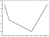
(a) The original function $f(x)$

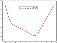
(b) The smoothed function $f^{\epsilon}(x)$

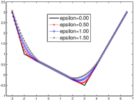
(c) Different smooth. parameters

Figure 1: The smoothing technique

Example 3 (Smoothing of a convex function).

Consider the following piecewise linear function

$$f(x)=\left\{\begin{array}[]{ll}-2x-3&\hbox{for }x<-2,\cr-0.3x+0.4&\hbox{for }-2\leq x<3\cr x-3.5&\hbox{for }x\geq 3.\end{array}\right.$$

Suppose that $z$ is a uniform random variable defined on $[-\epsilon,\epsilon]$ where $\epsilon>0$ is a given parameter. Consider the approximation function $f^{\epsilon}=\mathsf{E}\!\left[f(x+z)\right]$. Proposition 5 implies that $f^{\epsilon}$ is a smooth function. When $\epsilon$ is a fixed constant satisfying $0<\epsilon\leq 2.5$, the smoothed function $f^{\epsilon}$ has the following form:

$$f^{\epsilon}(x)=\left\{\begin{array}[]{ll}-2x-3&\hbox{for }x<-2-\epsilon,\cr\frac{1}{40\epsilon}\left(17x^{2}+68x-46x\epsilon+68-52\epsilon+17\epsilon^{2}\right)&\hbox{for }-2-\epsilon\leq x<-2+\epsilon,\cr-0.3x+0.4&\hbox{for }-2+\epsilon\leq x<3-\epsilon,\cr\frac{1}{40\epsilon}\left(13x^{2}-78x+14x\epsilon+117-62\epsilon+13\epsilon^{2}\right)&\hbox{for }3-\epsilon\leq x<3+\epsilon,\cr x-3.5&\hbox{for }x\geq 3+\epsilon.\end{array}\right.$$

Figure 1 shows such a smoothing scheme. In Figure 1a, we observe that function $f$ is nonsmooth at $x=-2$ and $x=3$. Figure 1b shows the approximation $f^{\epsilon}$ when $\epsilon=0.5$. An immediate observation is that function $f^{\epsilon}$ is smooth everywhere. Furthermore, the smoothing technique perturbs $x$ locally at all points, including points of nonsmoothness. Finally, Figure 1c shows the smoothing scheme for different values of $\epsilon$ and illustrates the exactness of the approximation as $\epsilon\to 0$.

4.2 Locally randomized techniques

Motivated by the smoothing technique described in previous part, we introduce two distributed smoothing schemes where we simultaneously perturb the value of vectors $x_{i}$ with a random vector $z_{i}$ for $i=1,\ldots,N$. The first scheme is called a multi-spherical randomized (MSR) scheme, where each random vector $z_{i}\in\mathbb{R}^{n_{i}}$ is uniformly distributed on the $n_{i}$-dimensional ball centered at the origin with radius $\epsilon_{i}$. In the second scheme, called a multi-cubic randomized (MCR) scheme, we let $z_{i}\in\mathbb{R}^{n_{i}}$ be uniformly distributed on the $n_{i}$-dimensional cube centered at the origin with an edge length of $2\epsilon_{i}$.

Now, consider a mapping $F$ that is not necessarily Lipschitz. We begin by defining an approximation $F^{\epsilon}:X\to\mathbb{R}^{n}$ as the expectation of $F(x)$ when $x$ is perturbed by a random vector $z=(z_{1};\ldots;z_{N})$. Specifically, $F^{\epsilon}$ is given by

$$F^{\epsilon}(x)\triangleq\begin{pmatrix}\mathsf{E}\!\left[F_{1}(x+z)\right]\\ \vdots\\ \mathsf{E}\!\left[F_{N}(x+z)\right]\end{pmatrix}\qquad\hbox{for all }x\in X,$$ (28)

where $F_{1},\ldots,F_{N}$ are coordinate-maps of $F$, $z=(z_{1};\ldots;z_{N})$ and the random vectors $z_{i}$ are given by MSR or MCR scheme.

4.2.1 Multi-spherical randomized smoothing

Let us define $B_{n}(x,\rho)\subset\mathbb{R}^{n}$ as a ball centered at a point $x$ with a radius $\rho>0$. More precisely,

$$B_{n}(x,\rho)\triangleq\{y\in\mathbb{R}^{n}\mid\|y-x\|\leq\rho\}.$$

In this scheme, assume that for all $i=1,\ldots,N$ random vector $z_{i}\in B_{n_{i}}(0,\epsilon_{i})$ is uniformly distributed and independent with respect to random vectors $z_{j}$ for $j\neq i$. For the approximation mapping $F^{\epsilon}$ to be well-defined, $F$ needs to be defined over the set $X_{S}^{\epsilon}$ given by

$$X_{s}^{\epsilon}\triangleq X+\prod_{i=1}^{N}B_{n_{i}}(0,\epsilon_{i}).$$

This means that $X_{s}^{\epsilon}=\{(x_{1}+z_{1},\ldots,x_{N}+z_{N}){{\color[rgb]{0,0,0}\mid}}x\in X,z_{i}\in\mathbb{R}^{n_{i}},\|z_{i}\|\leq\epsilon_{i}\,\hbox{ for all }i=1,\ldots,N\},$ where the constants $\epsilon_{i}>0$ are given values and $\epsilon\triangleq(\epsilon_{1},\ldots,\epsilon_{N}).$ Note that the subscript $s$ stands for the MSR scheme. This scheme is developed based on the following assumption.

Assumption 4.

The mapping $F:X_{s}^{\epsilon}\to\mathbb{R}^{n}$ is bounded over the set $X_{s}^{\epsilon}$. In particular, for every $i=1,\ldots,N$, there exists a constant $C_{i}>0$ such that $\|F_{i}(x)\|\leq C_{i}$ for all $x\in X_{s}^{\epsilon}$.

Under this assumption, we will show that the smoothed mapping $F^{\epsilon}$ produced by the MSR scheme is Lipschitz continuous over $X$ and we will compute its Lipschitz constant. To do so, we make use of the following lemma.

Lemma 6.

Let $z\in\mathbb{R}^{n}$ be a random vector generated from a uniform density with zero mean over an $n$-dimensional ball centered at the origin with a radius $\epsilon$. Then, the following relation holds:

$$\int_{\mathbb{R}^{n}}|p{{}_{u}}(z-x)-p{{}_{u}}(z-y)|dz\leq\kappa\frac{n!!}{(n-1)!!}\,\frac{\|x-y\|}{\epsilon}\qquad\hbox{for all }x,y\in\mathbb{R}^{n},$$

where $\kappa=1$ if $n$ is odd and $\kappa=\frac{2}{\pi}$ if $n$ is even, $n!!$ denotes double factorial of $n$, and $p_{u}$ is the probability density function of random vector $z$ given by

$$p{{}_{u}}(z)=\left\{\begin{array}[]{ll}\frac{1}{c_{n}\varepsilon^{n}}&\hbox{for }z\in B_{n}(0,\epsilon),\cr\hbox{}&\hbox{}\cr 0&\hbox{otherwise,}\end{array}\right.$$ (29)

where $c_{n}=\dfrac{\pi^{\frac{n}{2}}}{\Gamma(\frac{n}{2}+1)}$, and $\Gamma$ is the gamma function given by

$$\Gamma\left(\frac{n}{2}+1\right)=\left\{\begin{array}[]{ll}\left(\frac{n}{2}\right)!&\hbox{if $n$ is even,}\cr\hbox{}&\hbox{}\cr\sqrt{\pi}\,\frac{n!!}{2^{(n+1)/2}}&\hbox{if $n$ is odd}.\end{array}\right.$$

Proof.

The result is shown within the proof of Lemma 8 in the extended version of [41]. ∎

We next provide the main result of this subsection, which establishes the Lipschitz continuity and boundedness properties of the approximation mapping $F^{\epsilon}$. It also provides the Lipschitz constant of $F^{\epsilon}$ for the MSR scheme in terms of problem parameters.

Proposition 6 (Lipschitz continuity and boundedness of $F^{\epsilon}$ under the MSR scheme).

Let Assumption 4 hold and define vector $C\triangleq(C_{1},\ldots,C_{N})$. Then, for any $\epsilon=(\epsilon_{1},\ldots,\epsilon_{N})>0$ we have the following:

• $F^{\epsilon}$ is bounded over the set $X$, i.e, $\|F^{\epsilon}(x)\|\leq\|C\|$ for all $x\in X$.

• $F^{\epsilon}$ is Lipschitz continuous over the set $X$. More precisely, we have

  $$\|F^{\epsilon}(x)-F^{\epsilon}(y)\|\leq{\sqrt{N}}\|C\|\max_{j\in\{1,\ldots,N\}}\left\{{\kappa_{j}}\frac{n_{j}!!}{(n_{j}-1)!!}\,\frac{1}{\epsilon_{j}}\right\}\|x-y\|\qquad\hbox{for all }x,y\in X,$$ (31)

  where $\kappa_{j}=1$ when $n_{j}$ is odd and $\kappa_{j}=\frac{2}{\pi}$ when $n_{j}$ is even.

Proof.

(a)  We can bound the norm of $F^{\epsilon}$ as follows:

$$\|F^{\epsilon}(x)\|=\sqrt{\sum_{i=1}^{N}\|\mathsf{E}\!\left[F_{i}(x+z)\right]\|^{2}}\leq\sqrt{\sum_{i=1}^{N}\mathsf{E}\!\left[\|F_{i}(x+z)\|^{2}\right]}\leq\|C\|,$$

where the first inequality follows from Jensen’s inequality and the second inequality is due to the boundedness property imposed on $F$ by Assumption 4.

(b)  From the definition of $F^{\epsilon}$ in relation (28) we have

$$\|F^{\epsilon}(x)-F^{\epsilon}(y)\|^{2}=\sum_{j=1}^{N}\|\mathsf{E}\!\left[F_{j}(x+z)-F_{j}(y+z)\right]\|^{2}=\sum_{j=1}^{N}\|\mathsf{E}\!\left[F_{j}(x+z)-F_{j}(y+z)\right]\|^{2}.$$

We will add and subtract, sequentially, the values $F(u)$ at the vectors $u$ of the form $(y_{1}+z_{1},\ldots,y_{i-1}+z_{i-1},x_{i}+z_{i},\ldots,x_{N}+z_{N})$ for $i=2,\ldots,N$. To keep the resulting expressions in a compact form, we use the following notation. For an index set $J\subseteq\{1,\ldots,N\}$, we let $x_{J}\triangleq(x_{i})_{i\in J}$ and $x_{-J}\triangleq(x_{i})_{i\in\{1,\ldots,N\}-J}$. By adding and subtracting the terms $F_{j}((y+z)_{\{1,\ldots,i\}},(x+z)_{-\{1,\ldots,i\}})$ for all $i$, from the preceding relation we obtain

$$\quad\|F^{\epsilon}(x)-F^{\epsilon}(y)\|^{2}=\sum_{j=1}^{N}\left\|\underbrace{\mathsf{E}\!\left[F_{j}(x+z)-F_{j}((y+z)_{\{1\}},(x+z)_{-\{1\}})\right]}_{v_{1}}\right.$$

$$+ \left.\underbrace{\mathsf{E}\!\left[F_{j}((y+z)_{\{1\}},(x+z)_{-\{1\}})-F_{j}((y+z)_{\{1,2\}},(x+z)_{-\{1,2\}})\right]}_{v_{2}}\right.$$

$$\left.\vdots\right.$$

$$+ \left.\underbrace{\mathsf{E}\!\left[F_{j}((y+z)_{\{1,\ldots,i-1\}},(x+z)_{-\{1,\ldots,i-1\}})-F_{j}((y+z)_{\{1,\ldots,i\}},(x+z)_{-\{1,\ldots,i\}})\right]}_{v_{i}}\right.$$

$$\left.\vdots\right.$$

$$+ \left.\underbrace{\mathsf{E}\!\left[F_{j}((y+z)_{\{1,\ldots,N-2\}},(x+z)_{-\{1,\ldots,N-2\}})-F_{j}((y+z)_{\{1,\ldots,N-1\}},(y+z)_{-\{1,\ldots,N-1\}})\right]}_{v_{N-1}}\right.$$

$$+ \left.\underbrace{\mathsf{E}\!\left[F_{j}((y+z)_{\{1,\ldots,N-1\}},(x+z)_{-\{1,\ldots,N-1\}})-F_{j}(y+z)\right]}_{v_{N}}\right\|^{2}.$$

Considering the definition of the vectors $v_{1},\ldots,v_{N}$ in the preceding relation, we have

$$\|F^{\epsilon}(x)-F^{\epsilon}(y)\|^{2}=\sum_{j=1}^{N}\left\|\sum_{i=1}^{N}v_{i}\right\|^{2}\leq N\sum_{j=1}^{N}\sum_{i=1}^{N}\|v_{i}\|^{2},$$

where the inequality follows by the convexity of the squared-norm. By using the definitions of $v_{i}$ and exchanging the order of summations in the preceding relation, we obtain

$$\quad\|F^{\epsilon}(x)-F^{\epsilon}(y)\|^{2}\leq{N}\underbrace{\sum_{j=1}^{N}\left\|\mathsf{E}\!\left[F_{j}((x+z)_{\{1\}},(x+z)_{-\{1\}})-F_{j}((y+z)_{\{1\}},(x+z)_{-\{1\}})\right]\right\|^{2}}_{\rm Term\,1}$$

$$+{N}\sum_{i=2}^{N}\underbrace{\sum_{j=1}^{N}\left\|\mathsf{E}\!\left[F_{j}((y+z)_{\{1,\ldots,i-1\}},(x+z)_{-\{1,\ldots,i-1\}})-F_{j}((y+z)_{\{1,\ldots,i\}},(x+z)_{-\{1,\ldots,i\}})\right]\right\|^{2}}_{{\rm Term}\,i}.$$ (32)

Next, we derive an estimate for Term 1. From our notation, it follows that for a vector $x$, $x_{\{1\}}=x_{1}$. In the interest of brevity, in the following, for a vector $x$, we use $x_{-1}\triangleq x_{-\{1\}}$. Recalling the definition of $p_{u}$ in (29), we write

Term 1 $$=\sum_{j=1}^{N}\left\|\int_{\mathbb{R}^{n_{1}}}F_{j}(x_{1}+z_{1},x_{-1}+z_{-1})p_{u}(z_{1})dz_{1}-\int_{\mathbb{R}^{n_{1}}}F_{j}(y_{1}+z_{1},x_{-1}+z_{-1})p_{u}(z_{1})dz_{1}\right\|^{2}$$

$$=\sum_{j=1}^{N}\left\|\int_{\mathbb{R}^{n_{1}}}F_{j}(s_{1},x_{-1}+z_{-1})p_{u}(s_{1}-x_{1})ds_{1}-\int_{\mathbb{R}^{n_{1}}}F_{j}(t_{1},x_{-1}+z_{-1})p_{u}(t_{1}-y_{1})dt_{1}\right\|^{2}$$

$$=\sum_{j=1}^{N}\left\|\int_{\mathbb{R}^{n_{1}}}\mathsf{E}\!\left[F_{j}(t_{1},x_{-1}+z_{-1})\right](p_{u}(t_{1}-x_{1})-p_{u}(t_{1}-y_{1}))dt_{1}\right\|^{2},$$

where in the second equality $s_{1}$ and $t_{1}$ are given by $s_{1}=x_{1}+z_{1}$ and $t_{1}=y_{1}+z_{1}$. Using the triangle inequality and Jensen’s inequality, we obtain

$$\hbox{Term 1}\leq\sum_{j=1}^{N}\left(\int_{\mathbb{R}^{n_{1}}}\mathsf{E}\!\left[\|F_{j}(t_{1},x_{-1}+z_{-1})\|\right]\,|p_{u}(t_{1}-x_{1})-p_{u}(t_{1}-y_{1})|dt_{1}\right)^{2}.$$

By the definition of $F_{j}$ and Assumption 4, the preceding relation yields

Term 1 $$\leq\sum_{j=1}^{N}\left(\int_{\mathbb{R}^{n_{1}}}C_{j}\,|p_{u}(t_{1}-x_{1})-p_{u}(t_{1}-y_{1})|dt_{1}\right)^{2}$$

$$\leq\left(\sum_{j=1}^{N}C_{j}^{2}\right)\left(\kappa_{1}\frac{n_{1}!!}{(n_{1}-1)!!}\frac{1}{\epsilon_{1}}\|x_{1}-y_{1}\|\right)^{2},$$

where the last inequality is obtained using Lemma 6. Similarly, we may find estimates for the other terms in relation (4.2.1). Therefore, from relation (4.2.1) we may conclude that

$$\|F^{\epsilon}(x)-F^{\epsilon}(y)\|^{2} \leq N\left(\sum_{j=1}^{N}C_{j}^{2}\right)\sum_{i=1}^{N}\left(\kappa_{i}\frac{n_{i}!!}{(n_{i}-1)!!}\frac{1}{\epsilon_{i}}\|x_{i}-y_{i}\|\right)^{2}$$

$$\leq N\left(\sum_{j=1}^{N}C_{j}^{2}\right)\left(\max_{t=1,\ldots,N}\kappa_{t}\frac{n_{t}!!}{(n_{t}-1)!!}\frac{1}{\epsilon_{t}}\right)^{2}\sum_{i=1}^{N}\|x_{i}-y_{i}\|^{2}$$

$$=N\|C\|^{2}\left(\max_{t=1,\ldots,N}\kappa_{t}\frac{n_{t}!!}{(n_{t}-1)!!}\frac{1}{\epsilon_{t}}\right)^{2}\|x-y\|^{2}.$$

Therefore, we have

$$\|F^{\epsilon}(x)-F^{\epsilon}(y)\|\leq\sqrt{N}\|C\|\max_{t\in\{1,\ldots,N\}}\left\{\kappa_{t}\frac{n_{t}!!}{(n_{t}-1)!!}\frac{1}{\epsilon_{t}}\right\}\|x-y\|.$$

∎

Remark: The MSR scheme is a generalization of the local randomization smoothing scheme presented in [41]. Note that when $N=1$, the Lipschitz constant given in Proposition 6b is precisely the constant given by Lemma 8 in [41]. $\square$

4.2.2 Multi-cubic randomized smoothing scheme

We begin by defining $C_{n}(x,\rho)\subset\mathbb{R}^{n}$ as a cube centered at a point $x$ with the edge length $2\rho>0$ where the edges are along the coordinate axes. More precisely,

$$C_{n}(x,\rho)\triangleq\{y\in\mathbb{R}^{n}\mid\|y-x\|_{\infty}\leq\rho\}.$$

In the MCR scheme, we assume that for any $i=1,\ldots,N$, the random vector $z_{i}$ is uniformly distributed on the set $C_{n_{i}}(0,\epsilon_{i})$ and is independent of the other random vectors $z_{j}$ for $j\neq i$. For the mapping $F$ we will assume that it is well-defined over the set $X_{c}^{\epsilon}$ given by

$$X_{c}^{\epsilon}\triangleq X+\prod_{i=1}^{N}C_{n_{i}}(0,\epsilon_{i}),$$

where $\epsilon_{i}>0$ are given values and $\epsilon\triangleq(\epsilon_{1},\ldots,\epsilon_{N}),$ while the subscript $c$ stands for the MCR scheme. We investigate the properties of $F^{\epsilon}$ for this smoothing scheme under the following basic assumption.

Assumption 5.

The mapping $F:X_{c}^{\epsilon}\to\mathbb{R}^{n}$ is bounded over the set $X_{c}^{\epsilon}$. Specifically, for every $i=1,\ldots,N$, there exists a constant $C^{\prime}_{i}>0$ such that $\|F_{i}(x)\|\leq C^{\prime}_{i}$ for all $x\in X_{c}^{\epsilon}$.

The following lemma provides a simple relation that will be important in establishing the main property of the density function used in the MCR scheme.

Lemma 7.

Let the vector $p\in\mathbb{R}^{m}$ be such that $0\leq p_{i}\leq 1$ for all $i=1,\ldots,m$. Then, we have

$$1-\prod_{i=1}^{m}(1-p_{i})\leq\|p\|_{1}.$$

Proof.

We use induction on $m$ to prove this result. For $m=1$, we have $1-\prod_{i=1}^{m}(1-p_{i})=p_{1}=\|p\|_{1}$, implying that the result holds for $m=1$. Let us assume that $1-\prod_{i=1}^{m}(1-p_{i})\leq\|p\|_{1}$ holds for $m$. Therefore, we have

$$\prod_{i=1}^{m}(1-p_{i})\geq 1-\sum_{i=1}^{m}p_{i}.$$

Multiplying both sides of the preceding relation by $(1-p_{m+1})$, we obtain

$$\prod_{i=1}^{m+1}(1-p_{i})\geq(1-\sum_{i=1}^{m}p_{i})(1-p_{m+1})=1-\sum_{i=1}^{m+1}p_{i}+p_{m+1}\sum_{i=1}^{m}p_{i}\geq 1-\sum_{i=1}^{m+1}p_{i}.$$

Hence, $\prod_{i=1}^{m+1}(1-p_{i})\geq 1-\sum_{i=1}^{m+1}p_{i}$ which implies that the result holds for $m+1$. Therefore, we conclude that the result holds for any integer $m\geq 1$. ∎

The following result is crucial for establishing the properties of the approximation $F^{\epsilon}$ obtained by the MCR smoothing scheme.

Lemma 8.

Let $z\in\mathbb{R}^{n}$ be a random vector with a zero-mean uniform density over an $n$-dimensional cube $\prod_{i=1}^{N}C_{n_{i}}(0,\epsilon_{i})$ for $\epsilon_{i}>0$ for all $i$. Let the function $p_{c}:\mathbb{R}^{n}\rightarrow\mathbb{R}$ be the probability density function of the random vector $z$:

$$p_{c}(z)=\left\{\begin{array}[]{ll}\frac{1}{2^{n}\prod_{i=1}^{N}\epsilon_{i}^{n_{i}}}&\hbox{for }z\in\prod_{i=1}^{N}C_{n_{i}}(0,\epsilon_{i}),\cr\hbox{}&\hbox{}\cr 0&\hbox{otherwise.}\end{array}\right.$$

Then, the following relation holds:

$$\int_{\mathbb{R}^{n}}|p_{c}(u-x)-p_{c}(u-y)|du\leq\frac{\sqrt{n}}{\displaystyle\min_{1\leq i\leq N\}}\{\epsilon_{i}\}}\|x-y\|\qquad\hbox{for all }x,y\in\mathbb{R}^{n}.$$

Proof.

Let $x,y\in\mathbb{R}^{n}$ be arbitrary. To simplify the notation, we define sets $S_{x}=\prod_{i=1}^{N}C_{n_{i}}(x_{i},\epsilon_{i})$ and $S_{y}=\prod_{i=1}^{N}C_{n_{i}}(y_{i},\epsilon_{i})$. We consider, separately, the case when the cubes $S_{x}$ and $S_{y}$ do not intersect, and the case when they do intersect. Before we proceed, we prove the following relation

$$S_{x}\cap S_{y}\neq\emptyset\quad\hbox{if and only if}\quad\|x_{i}-y_{i}\|_{\infty}\leq 2\epsilon_{i}\ \hbox{for all }i=1,\ldots,N.$$ (33)

To prove relation (33), suppose that the two cubes have nonempty intersection and let $u$ be in the intersection, i.e., $u\in S_{x}\cap S_{y}$. Then, by the triangle inequality, we have for all $i=1,\ldots,N$,

$$\|x_{i}-y_{i}\|_{\infty}\leq\|x_{i}-u_{i}\|_{\infty}+\|u_{i}-y_{i}\|_{\infty}\leq 2\epsilon_{i},$$

where the last inequality follows from the fact that $u$ belongs to each of the two cubes. Thus, when $S_{x}\cap S_{y}\neq\emptyset$, we have $\|x_{i}-y_{i}\|_{\infty}\leq 2\epsilon_{i}$ for all $i$. Conversely, suppose now that $\|x_{i}-y_{i}\|_{\infty}\leq 2\epsilon_{i}$ holds for all $i=1,\ldots,N.$ Let $\bar{u}=(x+y)/2$, and note that by the convexity of the norm $\|\cdot\|_{\infty}$, we have

$$\|\bar{u}_{i}-x_{i}\|_{\infty}=\left\|\frac{y-x}{2}\right\|_{\infty}\leq\frac{1}{2}\|y_{i}-x_{i}\|_{\infty}\leq\epsilon_{i}\qquad\hbox{for all }i.$$

Thus, it follows that $\bar{u}\in S_{x}$. Similarly, we find that $\|\bar{u}_{i}-y_{i}\|_{\infty}\leq\epsilon_{i}$ for all $i$, which implies that $\bar{u}\in S_{y}$. Hence, $\bar{u}\in S_{x}\cap S_{y}$, thus showing that the two cubes have a nonempty intersection.

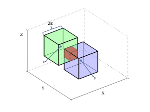
(a) MCR scheme

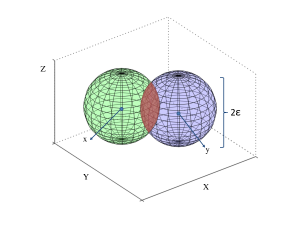
(b) MSR scheme

Figure 2: Calculating the Lipschitz constant in the locally randomized schemes.

We now consider the integral $\int_{\mathbb{R}^{n}}|p_{c}(u-x)-p_{c}(u-y)|du$ for the cases when the cubes do not intersect and when they do intersect.
Case 1: $S_{x}\cap S_{y}=\emptyset$. In this case, we have

$$\int_{S_{x}}|p_{c}(u-x)-p_{c}(u-y)|du =\int_{S_{x}}p_{c}(u-x)du,$$

$$\int_{S_{y}}|p_{c}(u-x)-p_{c}(u-y)|du =\int_{S_{y}}p_{c}(u-y)du.$$

Consequently

$$\int_{\mathbb{R}^{n}}|p_{c}(u-x)-p_{c}(u-y)|du=\int_{S_{x}}p_{c}(u-x)du+\int_{S_{y}}p_{c}(u-y)du=2.$$ (34)

By relation (33), there must exist some index $i^{*}\in\{1,\ldots,N\}$ such that $\|x_{i^{*}}-y_{i^{*}}\|_{\infty}>2\epsilon_{i^{*}}$. Since $\|x-y\|_{\infty}\geq\|x_{i^{*}}-y_{i^{*}}\|_{\infty}$, it follows that $\frac{\|x-y\|_{\infty}}{\min_{1\leq i\leq N}\{\epsilon_{i}\}}>2$. Using the relationship $\|u\|_{\infty}\leq\|u\|$ between the infinity-norm and the Euclidean norm, we obtain $\frac{\|x-y\|}{\min_{1\leq i\leq N}\{\epsilon_{i}\}}>2$. Therefore, using (34), we have

$$\int_{\mathbb{R}^{n}}|p_{c}(u-x)-p_{c}(u-y)|du<\frac{1}{\displaystyle\min_{1\leq i\leq N}\{\epsilon_{i}\}}\|x-y\|.$$ (35)

Case 2: $S_{x}\cap S_{y}\neq\emptyset$. Then, we may decompose the integral as follows:

$$\int_{\mathbb{R}^{n}}|p_{c}(u-x)-p_{c}(u-y)|du =\int_{S_{x}\cap S_{y}}|p_{c}(u-x)-p_{c}(u-y)|du+\int_{S_{x}^{c}\cap S_{y}^{c}}|p_{c}(u-x)-p_{c}(u-y)|du$$

$$+\int_{S_{x}\setminus S_{y}}|p_{c}(u-x)-p_{c}(u-y)|du+\int_{S_{y}\setminus S_{x}}|p_{c}(u-x)-p_{c}(u-y)|du.$$

Note that the first two integrals on the right hand side of the preceding equality are zero since $p_{c}(u-x)=p_{c}(u-y)$ in the corresponding regions. Figure 2a illustrates this observation. Therefore, we have

$$\int_{\mathbb{R}^{n}}|p_{c}(u-x)-p_{c}(u-y)|du =\int_{S_{x}\setminus S_{y}}p_{c}(u-x)du+\int_{S_{y}\setminus S_{x}}p_{c}(u-y)du=2\,\frac{1}{2^{n}\prod_{i=1}^{N}\epsilon_{i}^{n_{i}}}\int_{S_{x}\setminus S_{y}}du.$$

Note that the value $2^{n}\prod_{i=1}^{N}\epsilon_{i}^{n_{i}}$ is the volume of the cube $S_{x}$, denoted by ${\rm vol}(S_{x})$. Similarly, the integral $\int_{S_{x}\setminus S_{y}}du$ is equal to the volume of the set $S_{x}\setminus S_{y}$. Thus, we can write

$$\int_{\mathbb{R}^{n}}|p_{c}(u-x)-p_{c}(u-y)|du=2\frac{{\rm vol}(S_{x}\setminus S_{y})}{{\rm vol}(S_{x})}=2\frac{{\rm vol}(S_{x})-{\rm vol}(S_{x}\cap S_{y})}{{\rm vol}(S_{x})}=2\left(1-\frac{{\rm vol}(S_{x}\cap S_{y})}{{\rm vol}(S_{x})}\right).$$

It can be seen that

$${\rm vol}(S_{x}\cap S_{y})=\prod_{i=1}^{N}\prod_{j=1}^{n_{i}}(2\epsilon_{i}-|x_{i}(j)-y_{i}(j)|),$$

where $w(j)$ denotes the $j$-th coordinate value of a vector $w$. Therefore, from the preceding two relations and ${\rm vol}(S_{x})=2^{n}\prod_{i=1}^{N}\epsilon_{i}^{n_{i}}$ we find that

$$\int_{\mathbb{R}^{n}}|p_{c}(u-x)-p_{c}(u-y)|du =2\left(1-\frac{1}{2^{n}\prod_{i=1}^{N}\epsilon_{i}^{n_{i}}}\left(\prod_{i=1}^{N}\prod_{j=1}^{n_{i}}(2\epsilon_{i}-|x_{i}(j)-y(j)|)\right)\right)$$ (36)

$$=2\left(1-\prod_{i=1}^{N}\prod_{j=1}^{n_{i}}\left(1-\frac{|x_{i}(j)-y_{i}(j)|}{2\epsilon_{i}}\right)\right).$$ (37)

Since the cubes $S_{x}$ and $S_{y}$ do intersect, by relation (33) there must hold $\|x_{i}-y_{i}\|_{\infty}\leq 2\epsilon_{i}$ for all $i$. Hence. $0\leq\frac{|x_{i}(j)-y_{i}(j)|}{2\epsilon_{i}}\leq 1$ for all $i$. Now, invoking Lemma 7, from (36) we obtain

$$\int_{\mathbb{R}^{n}}|p_{c}(u-x)-p_{c}(u-y)|du\leq 2\sum_{i=1}^{N}\sum_{j=1}^{n_{i}}\frac{|x_{i}(j)-y_{i}(j)|}{2\epsilon_{i}}=\sum_{i=1}^{N}\frac{\|x_{i}-y_{i}\|_{1}}{\epsilon_{i}}\leq\sum_{i=1}^{N}\frac{\sqrt{n_{i}}}{\epsilon_{i}}\,\|x_{i}-y_{i}\|,$$

where in the last inequality we used the relation between $\|\cdot\|_{1}$ and the Euclidean norm. Using Hölder’s inequality, we have

$$\sum_{i=1}^{N}\frac{\sqrt{n_{i}}}{\epsilon_{i}}\,\|x_{i}-y_{i}\|\leq\sqrt{\sum_{i=1}^{N}\frac{n_{i}}{\epsilon^{2}_{i}}}\ \|x-y\|\leq\frac{\sqrt{n}}{\displaystyle\min_{1\leq i\leq N}\{\epsilon_{i}\}}\|x-y\|,$$

implying that

$$\int_{\mathbb{R}^{n}}|p_{c}(u-x)-p_{c}(u-y)|du\leq\frac{\sqrt{n}}{\displaystyle\min_{1\leq i\leq N\}}\{\epsilon_{i}\}}\|x-y\|.$$ (38)

By combining (40), (35), and (38), and using the fact $n\geq 1$, we obtain the desired result. ∎

Analogous to Proposition 6, the next proposition derives the Lipschitz constant and boundedness properties of the approximation $F^{\epsilon}$ under the MCR scheme.

Proposition 7 (Lipschitz continuity and boundedness of $F^{\epsilon}$ under the MCR scheme).

Let Assumption 5 hold and define vector $C^{\prime}\triangleq(C_{1}^{\prime},\ldots,C_{N}^{\prime})$. Then, for any $\epsilon=(\epsilon_{1},\ldots,\epsilon_{N})>0$ we have the following:

• $F^{\epsilon}$ is bounded over the set $X$, i.e., $\|F^{\epsilon}(x)\|\leq\|C^{\prime}\|$ for all $x\in X$.

• $F^{\epsilon}$ is Lipschitz over the set $X$. More precisely, we have

  $$\|F^{\epsilon}(x)-F^{\epsilon}(y)\|\leq\frac{\sqrt{n}\|C^{\prime}\|}{\min_{j=1,\ldots,N}\{\epsilon_{j}\}}\|x-y\|\qquad\hbox{for all }x,y\in X.$$ (39)

Proof.

(a)  This result can be shown in a similar fashion to the proof of Proposition 6a.

(b)  Since the random vector $z_{i}$ is uniformly distributed on the set $C_{n_{i}}(0,\epsilon_{i})$ for each $i=1,\ldots,N$, the random vector $z=(z_{1};\ldots;z_{N})$ is uniformly distributed on the set $\prod_{i=1}^{N}C_{n_{i}}(0,\epsilon_{i})$. By the definition of the approximation $F^{\epsilon}$ in (28), it follows that for any $x,y\in X$,

$$\|F^{\epsilon}(x)-F^{\epsilon}(y)\| =\left\|\int_{\mathbb{R}^{n}}{F(x+z)}p_{c}(z)dz-\int_{\mathbb{R}^{n}}{F(y+z)}p_{c}(z)dz\right\|$$

$$=\left\|\int_{\mathbb{R}^{n}}{F(u)}p_{c}(u-x)du-\int_{\mathbb{R}^{n}}{F(v)}p_{c}(v-y)dv\right\|$$

$$=\left\|\int_{\mathbb{R}^{n}}{F(u)}(p_{c}(u-x)-p_{c}(u-y))du\right\|$$

$$\leq\int_{\mathbb{R}^{n}}\|F(u)\||p_{c}(u-x)-p_{c}(u-y)|du,$$

where in the second equality we let $u=x+z$ and $v=y+z$, while the inequality follows from the triangle inequality. Invoking Assumption 5 we obtain

$$\|F^{\epsilon}(x)-F^{\epsilon}(y)\|\leq\|C^{\prime}\|\int_{\mathbb{R}^{n}}|p_{c}(u-x)-p_{c}(u-y)|du.$$ (40)

The desired relation follows from relation (40) and Lemma 8. ∎

4.3 A distributed locally randomized SA scheme

The locally randomized schemes presented in Section 4.2 facilitate the construction of a distributed locally randomized SA scheme. Consider the Cartesian stochastic variational inequality problem VI$(X,F^{\epsilon})$ given in (28) where the mapping $F$ is not necessarily Lipschitz. In this section, we assume that the conditions of the MSR scheme are satisfied, i.e., for all $i=1,\ldots,N$, the random vector $z_{i}$ is uniformly distributed over the set $\in B_{n_{i}}(0,\epsilon_{i})$ independently from the other random vectors $z_{j}$ for $j\neq i$, and the mapping $F$ in (2) is defined over the set $X_{s}^{\epsilon}$. Let the sequence $\{x_{k}\}$ be given by

$$\begin{aligned} x_{{k+1},i}=\Pi_{X_{i}}\left(x_{k,i}-\gamma_{k,i}\Phi_{i}(x_{k}+z_{k},\xi_{k})\right),\end{aligned}$$ (41)

for all $k\geq 0$ and $i=1,\ldots,N$, where $\gamma_{k,i}>0$ denotes the stepsize of the $i$-th agent at iteration $k$, $x_{k}=(x_{k,1};x_{k,2};\ldots;x_{k,N})$, and $z_{k}=(z_{k,1};z_{k,2};\ldots;z_{k,N})$. The following proposition proves the almost-sure convergence of the iterates generated by algorithm (41) to the solution of the approximation VI$(X,F^{\epsilon})$. In this result, we proceed to show that the approximation does indeed satisfy the assumptions of Proposition 3 and convergence can then be immediately claimed. We define $\mathcal{F}^{\prime}_{k}$, the history of the method up to time $k$, as

$$\mathcal{F}^{\prime}_{k}\triangleq\{x_{0},z_{0},\xi_{0},z_{1},\xi_{1},\ldots,z_{k-1},\xi_{k-1}\},$$

for $k\geq 1$ and $\mathcal{F}^{\prime}_{0}=\{x_{0}\}$. We assume that, at any iteration $k$, the vectors $z_{k}$ and $\xi_{k}$ in (41) are independent given the history $\mathcal{F}^{\prime}_{k}$.

Proposition 8 (Almost-sure convergence of locally randomized DASA scheme).

Let Assumptions 1a, 3, and 4 hold, and suppose that mapping $F$ is strongly monotone on the set $X_{s}^{\epsilon}$ with a constant $\eta>0$. Also, assume that, for each $i=1,\ldots,N$, there exists a constant $\nu_{i}>0$ such that

$$\mathsf{E}\!\left[\|\Phi_{i}(x_{k}+z_{k},\xi_{k})-F_{i}(x_{k}+z_{k})\|^{2}\mid\mathcal{F}^{\prime}_{k}\right]\leq\nu_{i}^{2}\qquad a.s.\hbox{ for all $k$.}$$ (42)

Then, the sequence $\{x_{k}\}$ generated by algorithm (41) converges almost surely to the unique solution of VI$(X,F^{\epsilon})$.

Proof.

Define random vector $\xi^{\prime}\triangleq(z_{1};z_{2};\ldots;z_{N};\xi)$, allowing us to rewrite algorithm (41) as follows:

$$\begin{aligned} x_{{k+1},i}&=\Pi_{X_{i}}\left(x_{k,i}-\gamma_{k,i}(F_{i}^{\epsilon}(x_{k})+w_{k,i}^{\prime})\right),\cr w_{k,i}^{\prime}&\triangleq\Phi_{i}(x_{k}+z_{k},\xi_{k})-F_{i}^{\epsilon}(x_{k}).\end{aligned}$$ (43)

To prove convergence of the iterates produced by (43), it suffices to show that the conditions of Proposition 3 are satisfied for the set $X$, the mapping $F^{\epsilon}$, and the stochastic errors $w_{k,i}^{\prime}$.

(i) Since Assumption 4 holds, Proposition 6b implies that the mapping $F^{\epsilon}$ is Lipschitz over the set $X$ with the constant $\sqrt{N}\|C\|\max_{1\leq j\leq N}\{\kappa_{j}\frac{n_{j}!!}{(n_{j}-1)!!}\,\frac{1}{\epsilon_{j}}\}$. Thus, Assumption 1b holds for the mapping $F^{\epsilon}$.

(ii) Next, we show that the mapping $F^{\epsilon}$ is strongly monotone over $X$. Since the mapping $F$ is strongly monotone over the set $X_{s}^{\epsilon}$ with a constant $\eta>0$, for any $u,v\in X_{s}^{\epsilon}$, we have

$$(u-v)^{T}(F(u)-F(v))\geq\eta\|u-v\|^{2}.$$

Therefore, for any $x,y\in X$ and any realization of the random vector $z$, the vectors $x+z$ and $y+z$ belong to the set $X_{s}^{\epsilon}$. Consequently, by defining $u\triangleq x+z$ and $v\triangleq y+z$, respectively, and nothing that $u-v=x-y$, from the previous relation we obtain

$$(x-y)^{T}(F(x+z)-F(y+z))\geq\eta\|x-y\|^{2}.$$

Taking expectations on both sides, it follows that

$$(x-y)^{T}\left(\mathsf{E}\!\left[F(x+z)\right]-\mathsf{E}\!\left[F(y+z)\right]\right)\geq\eta\|x-y\|^{2},$$

which implies that $F^{\epsilon}$ is strongly monotone over the set $X$ with the constant $\eta$.

(iii) The last step of the proof entails showing that the stochastic errors $w_{k}^{\prime}\triangleq(w_{k,1};w_{k,2};\ldots;w_{k,N})$ are well-defined, i.e., $\mathsf{E}\!\left[w_{k}^{\prime}\mid\mathcal{F}^{\prime}_{k}\right]=0$ and that Assumption 2 holds with respect to the stochastic error $w_{k}^{\prime}$. Consider the definition of $w_{k,i}^{\prime}$ in (43). Taking conditional expectations on both sides, we have for all $i=1,\ldots,N$

$$\mathsf{E}\!\left[w_{k,i}^{\prime}\mid\mathcal{F}^{\prime}_{k}\right]={\mathsf{E}_{z,\xi}\!\left[\Phi_{i}(x_{k}+z_{k},\xi_{k})\right]}-F_{i}^{\epsilon}(x_{k})=\mathsf{E}\!\left[F_{i}(x_{k}+z_{k})\right]-F_{i}^{\epsilon}(x_{k})=F_{i}^{\epsilon}(x_{k})-F_{i}^{\epsilon}(x_{k})=0,$$

where the last equality is obtained using the definition of $F^{\epsilon}$ in (28). Consequently, it suffices to show that the condition of Assumption 2 holds. This may be expressed as follows:

$$\mathsf{E}\!\left[\|w_{k}^{\prime}\|^{2}\mid\mathcal{F}^{\prime}_{k}\right] =\mathsf{E}\!\left[\sum_{i=1}^{N}\|w_{k,i}^{\prime}\|^{2}\mid\mathcal{F}^{\prime}_{k}\right]=\mathsf{E}_{z,\xi}\!\left[\sum_{i=1}^{N}\|\Phi_{i}(x_{k}+z_{k},\xi_{k})-F_{i}^{\epsilon}(x_{k})\|^{2}\mid\mathcal{F}^{\prime}_{k}\right].$$

By adding and subtracting $F_{i}(x_{k}+z_{k})$ we obtain

$$\mathsf{E}\!\left[\|w_{k}^{\prime}\|^{2}\mid\mathcal{F}^{\prime}_{k}\right]\leq 2\mathsf{E}_{z,\xi}\!\left[\sum_{i=1}^{N}\left(\|\Phi_{i}(x_{k}+z_{k},\xi_{k})-F_{i}(x_{k}+z_{k})\|^{2}+\|F_{i}(x_{k}+z_{k})-F_{i}^{\epsilon}(x_{k})\|^{2}\right)\mid\mathcal{F}^{\prime}_{k}\right]$$

$$= 2\sum_{i=1}^{N}\mathsf{E}\!\left[\mathsf{E}\!\left[\|\Phi_{i}(x_{k}+z_{k},\xi_{k})-F_{i}(x_{k}+z_{k})\|^{2}\mid\mathcal{F}^{\prime}_{k},z_{k}\right]\mid\mathcal{F}^{\prime}_{k}\right]$$

$$+2\sum_{i=1}^{N}\mathsf{E}\!\left[(\|F_{i}(x_{k}+z_{k})\|^{2}-\|F_{i}^{\epsilon}(x_{k})\|^{2})\mid\mathcal{F}^{\prime}_{k}\right],$$

where the last term is obtained from the following relation:

$$\mathsf{E}\!\left[F_{i}(x_{k}+z_{k})^{T}F^{\epsilon}(x_{k})\mid\mathcal{F}_{k}^{\prime}\right]=\mathsf{E}\!\left[F_{i}(x_{k}+z_{k})^{T}F^{\epsilon}(x_{k})\mid x_{k}\right]=\|F^{\epsilon}(x_{k})\|^{2}.$$

Using the assumption on the errors given in (42), we further obtain

$$\mathsf{E}\!\left[\|w_{k}^{\prime}\|^{2}\mid\mathcal{F}^{\prime}_{k}\right]\leq 2\sum_{i=1}^{N}\nu_{i}^{2}+2\sum_{i=1}^{N}\mathsf{E}\!\left[(\|F_{i}(x_{k}+z_{k})\|^{2}-\|F_{i}^{\epsilon}(x_{k})\|^{2})\mid\mathcal{F}^{\prime}_{k}\right].$$ (44)

Furthermore, we have

$$\sum_{i=1}^{N}\mathsf{E}\!\left[(\|F_{i}(x_{k}+z_{k})\|^{2}-\|F_{i}^{\epsilon}(x_{k})\|^{2})\mid\mathcal{F}^{\prime}_{k}\right]\leq\sum_{i=1}^{N}\mathsf{E}\!\left[\|F_{i}(x_{k}+z_{k})\|^{2}\mid\mathcal{F}^{\prime}_{k}\right]\leq C^{2},$$ (45)

where we use the fact $x_{k}+z_{k}\in X_{s}^{\epsilon}$ and the assumption that $F_{i}$ is uniformly bounded over the set $X_{s}^{\epsilon}$ (cf. Assumption 4). Relations (44)–(45) imply that the stochastic errors $\{w_{k}^{\prime}\}$ satisfy Assumption 2. Thus, the conditions of Proposition 3 are satisfied for the set $X$, the mapping $F^{\epsilon}$, and the stochastic errors $w_{k,i}^{\prime}$ and the convergence result follows. ∎

The distributed locally randomized SA scheme produces a solution that is an approximation to the true solution. A natural question is whether the sequence of approximations tends to the solution of VI$(X,F)$ as $\epsilon$, the size of the support of the randomization, tends to zero. The following proposition resolves this question in the affirmative.

Proposition 9.

Let Assumption 1a hold, and suppose that mapping $F$ is a continuous and strongly monotone over the set $X_{s}^{\epsilon}$. Let $x^{\epsilon}$ and $x^{*}$ denote the solution of VI$(X,F^{\epsilon})$ and VI$(X,F)$, respectively. Then $x^{\epsilon}\to x^{*}$ when $\epsilon\to 0$.

Proof.

As showed in the proof of Proposition 8, $F^{\epsilon}$ is also strongly monotone over the set $X$ with constant $\eta$. Since set $X$ is assumed to be closed and convex, the definition of $X_{s}^{\epsilon}$ implies that $X_{s}^{\epsilon}$ is also closed and convex. Thus, the existence and uniqueness of the solution to VI$(X,F)$, as well as VI$(X,F^{\epsilon})$, is guaranteed by Theorem 2.3.3 of [11].

Let $\epsilon=(\epsilon_{1},\epsilon_{2},\ldots,\epsilon_{N})$ with $\epsilon_{i}>0$ for all $i$ be arbitrary, and let $x^{\epsilon}$ denote the solution to VI$(X,F^{\epsilon})$. Let $x^{*}$ be the solution to VI$(X,F)$. Thus, since $x^{\epsilon}$ is the solution to VI$(X,F^{\epsilon})$, we have $(x^{*}-x^{\epsilon})^{T}F^{\epsilon}(x^{\epsilon})\geq 0.$ Similarly, since $x^{*}$ is the solution to VI$(X,F)$, we have $(x^{\epsilon}-x^{*})^{T}F(x^{*})\geq 0$. Adding the preceding two inequalities, we obtain for any $k\geq 0$,

$$(x^{*}-x^{\epsilon})^{T}(F^{\epsilon}(x^{\epsilon})-F(x^{*}))\geq 0.$$

Adding and subtracting the term $F^{\epsilon}(x^{*})$, we have

$$(x^{*}-x^{\epsilon})^{T}(F^{\epsilon}(x^{\epsilon})-F^{\epsilon}(x^{*}))+(x^{*}-x^{\epsilon})^{T}(F^{\epsilon}(x^{*})-F(x^{*}))\geq 0,$$

implying that

$$(x^{*}-x^{\epsilon})^{T}(F^{\epsilon}(x^{*})-F(x^{*}))\geq(x^{*}-x^{\epsilon})^{T}(F^{\epsilon}(x^{*})-F^{\epsilon}(x^{\epsilon}))\geq\eta\|x^{*}-x^{\epsilon}\|^{2},$$

where the last inequality follows by the strong monotonicity of the mapping $F^{\epsilon}$. By invoking the Cauchy-Schwartz inequality, we obtain

$$\|F^{\epsilon}(x^{*})-F(x^{*})\|\geq\eta\|x^{*}-x^{\epsilon}\|.$$ (46)

Next, we show that $\lim_{\epsilon\to 0}F^{\epsilon}(x^{*})=F(x^{*}).$ By the definition of $F^{\epsilon}$ and Jensen’s inequality, we have

$$\|F^{\epsilon}(x^{*})-F(x^{*})\|=\|\mathsf{E}\!\left[F(x^{*}+z)-F(x^{*})\right]\|\leq\mathsf{E}\!\left[\|F(x^{*}+z)-F(x^{*})\|\right].$$ (47)

Then, the expectation on the right-hand side can be expressed as follows:

$$\mathsf{E}\!\left[\|F(x^{*}+z)-F(x^{*})\|\right] =\int_{\mathbb{R}^{n_{1}}}\ldots\int_{\mathbb{R}^{n_{N}}}\|F(x^{*}+z)-F(x^{*})\|\left(\prod_{i=1}^{N}p_{u}(z_{i})\right)dz_{1}\cdots dz_{N}$$ (48)

$$=\int_{{B_{n_{1}}(0,\epsilon_{1})}}\ldots\int_{{B_{n_{N}}(0,\epsilon_{N})}}\|F(x^{*}+z)-F(x^{*})\|\left(\prod_{i=1}^{N}p_{u}(z_{i})\right)dz_{1}\cdots dz_{N},\qquad$$ (49)

where the second equality is a consequence of the definition of the random vector $z$. Let $\delta>0$ be an arbitrary fixed number. By the continuity of $F$ over $X_{s}^{\epsilon}$, there exists a $\delta^{\prime}>0$, such that if $\|(x^{*}+z)-x^{*}\|\leq\delta^{\prime}$, then $\|F(x^{*}+z)-F(x^{*})\|\leq\delta$. Therefore, for all $\epsilon=(\epsilon_{1},\epsilon_{2},\ldots,\epsilon_{N})$ with $\|\epsilon\|\leq\delta^{\prime}$ we have $\|z\|\leq\|\epsilon\|\leq\delta^{\prime}$ for $z\in\prod_{i=1}^{N}B_{n_{i}}(0,\epsilon_{i})$, which is equivalent to $\|(x^{*}+z)-x^{*}\|\leq\delta^{\prime}$. Hence, $\|F(x^{*}+z)-F(x^{*})\|\leq\delta$ for all $z\in\prod_{i=1}^{N}B_{n_{i}}(0,\epsilon_{i})$ with $\epsilon_{i}$ such that $\|\epsilon\|\leq\delta^{\prime}$. Thus, using (47) and (48), for any $\epsilon=(\epsilon_{1},\ldots,\epsilon_{N})$ with $\|\epsilon\|\leq\delta^{\prime}$, we have

$$\|F^{\epsilon}(x^{*})-F(x^{*})\|\leq\delta{\int_{{B_{n_{1}}(0,\epsilon_{k,1})}}\ldots\int_{{B_{n_{N}}(0,\epsilon_{k,N})}}\left(\prod_{i=1}^{N}p_{u}(z_{i})\right)d{z_{k,1}}\ldots d{z_{k,N}}}=\delta.$$

Since $\delta>0$ was arbitrary, we conclude that $\lim_{\epsilon\to 0}\|F_{k}(x^{*})-F(x^{*})\|=0$. Therefore, taking limits on both sides of inequality (46), we obtain $\lim_{\epsilon\to 0}\|x^{*}-{x^{\epsilon_{k}}}\|=0$. ∎

Remark: Note that the results of Propostion 8 and Proposition 9 hold when the random vector $z$ fits the conditions of the MCR scheme.

5 Numerical results

In this section, we report the results of our numerical experiments on two sets of test problems. Of these, the first is a stochastic bandwidth-sharing problem in communication networks (Sec. 5.1), while the second is a stochastic Nash-Cournot game (Sec. 5.2). In each instance, we compare the performance of the distributed adaptive stepsize SA scheme (DASA) given by (26)–(27) with that of SA schemes with harmonic stepsize sequences (HSA), where agents use the stepsize $\frac{\theta}{k}$ at iteration $k$. More precisely, we consider three different values of the parameter $\theta$, i.e., $\theta=0.1$, $1$, and $10$. This diversity of choices allows us to observe the sensitivity of the HSA scheme to different settings of the parameters. In the context of Nash-Cournot games, we use the distributed locally randomized SA scheme described in Sec. 4.3 with the MSR and MCR techniques. In each instance, we conduct a sensitivity analysis where we consider $12$ different parameter settings, categorized into $4$ sets. In each set, one parameter is changed while other parameters are maintained as fixed. We provide $90\%$ confidence intervals of the mean squared error for each of the $12$ settings. Our experiments have been done using Matlab $7.12$.

5.1 A bandwidth-sharing problem in computer networks

We consider a communication network where users compete for the bandwidth. Such a problem can be captured by an optimization framework (cf. [6]). Motivated by this model, we consider a network with $16$ nodes, $20$ links and $5$ users. Figure 3 shows the configuration of this network.

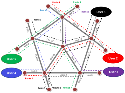
Figure 3: The bandwidth-sharing problem – the network

Users have access to different routes as shown in Figure 3. For example, user $1$ can access routes $1$, $2$, and $3$. Each user is characterized by a cost function. Additionally, there is a congestion cost function that depends on the aggregate flow. More specifically, the cost function user $i$ with flow rate (bandwidth) $x_{i}$ is defined by

$$f_{i}(x_{i},\xi_{i})\triangleq-\sum_{r\in\mathcal{R}(i)}\xi_{i}(r)\log(1+x_{i}(r)),$$

for $i=1,\ldots,5$, where $x\triangleq(x_{1};\ldots;x_{5})$ is the flow decision vector of the users, $\xi\triangleq(\xi_{1};\ldots;\xi_{5})$ is a random parameter corresponding to the different users, $\mathcal{R}(i)=\{1,2,\ldots,n_{i}\}$ is the set of routes assigned to the $i$-th user, $x_{i}(r)$ and $\xi_{i}(r)$ are the $r$-th element of the decision vector $x_{i}$ and the random vector $\xi_{i}$, respectively. We assume that $\xi_{i}(r)$ is drawn from a uniform distribution for each $i$ and $r$. More precisely, $\xi_{1}(1)$, $\xi_{1}(2)$, and $\xi_{1}(3)$ are i.i.d. and uniformly distributed in $[1-0.1,1+0.1]$, $\xi_{2}(1)$ and $\xi_{2}(2)$ are i.i.d. and uniformly distributed in $[1.4-0.2,1.4+0.2]$, $\xi_{3}(1)$ and $\xi_{4}(1)$ are i.i.d. and uniformly distributed in $[0.8-0.05,0.8+0.05]$ and $[1.6-0.2,1.6+0.2]$, respectively, and $\xi_{5}(1)$ and $\xi_{5}(2)$ are i.i.d and uniformly distributed in $[1.2-0.1,1.2+0.1]$.

The links have limited capacities, which are given by

$$b=(10;15;15;20;10;10;20;30;25;15;20;15;10;10;15;15;20;20;25;40).$$

We may define the routing matrix $A$ that describes the relation between set of routes $\mathcal{R}=\{1,2,\ldots,9\}$ and set of links $\mathcal{L}=\{1,2,\ldots,20\}$. Assume that $A_{lr}=1$ if route $r\in\mathcal{R}$ goes through link $l\in\mathcal{L}$ and $A_{lr}=0$ otherwise. Using this matrix, the capacity constraints of the links can be described by $Ax\leq b$.

We formulate this model as a stochastic optimization problem given by

minimize $$\sum_{i=1}^{N}\mathsf{E}\!\left[f_{i}(x_{i},\xi_{i})\right]+c(x)$$ (50)

subject to $$Ax\leq b$$

$$x\geq 0,$$

where $c(x)$ is the network congestion cost. We consider this cost of the form $c(x)=\|Ax\|^{2}$. Problem (50) is a convex optimization problem and the optimality conditions can be stated as a variational inequality given by $\nabla f(x^{*})^{T}(x-x^{*})\geq 0$, where $f(x)\triangleq\sum_{i=1}^{N}\mathsf{E}\!\left[f_{i}(x_{i},\xi_{i})\right]+c(x)$. Using our notation in Sec. 2.2, we have

$$F(x)\triangleq\nabla f(x)=-\left(\frac{\bar{\xi}_{1}(1)}{1+x_{1}(1)};\ldots;\frac{\bar{\xi}_{i}(r_{i})}{1+x_{i}(r_{i})};\ldots;\frac{\bar{\xi}_{5}(2)}{1+x_{5}(2)}\right)+2A^{T}Ax,$$

where $\bar{\xi}_{i}(r_{i})\triangleq\mathsf{E}\!\left[\xi_{i}(r_{i})\right]$ for any $i=1,\ldots,5$ and $r_{i}=1,\ldots,n_{i}$. We now show that the mapping $F$ is Lipschitz and strongly monotone. Using the preceding relation, triangle inequality, and Cauchy-Schwartz inequality, for any $x,y\in X\triangleq\{x\in\mathbb{R}^{N}|Ax\leq b,x\geq 0\}$, we have

$$\|F(x)-F(y)\|$$

$$=\left\|-\left(\bar{\xi}_{1}(1)\left(\frac{1}{1+x_{1}(1)}-\frac{1}{1+y_{1}(1)}\right);\ldots;\bar{\xi}_{5}(2)\left(\frac{1}{1+x_{5}(2)}-\frac{1}{1+y_{5}(2)}\right)\right)+2A^{T}A(x-y)\right\|$$

$$\leq\left\|\left(\bar{\xi}_{1}(1)\frac{x_{1}(1)-y_{1}(1)}{(1+x_{1}(1))(1+y_{1}(1))};\ldots;\bar{\xi}_{5}(2)\frac{x_{5}(2)-y_{5}(2)}{(1+x_{5}(2))(1+y_{5}(2))}\right)\right\|+2\|A^{T}A\|\|x-y\|.$$

Using nonnegativity constraints, from the preceding relation we obtain

$$\|F(x)-F(y)\|\leq\max_{i,r_{i}}\bar{\xi}_{i}(r_{i})\|x-y\|+2\|A^{T}A\|\|x-y\|=\left(\max_{i,r_{i}}\bar{\xi}_{i}(r_{i})+2\|A^{T}A\|\right)\|x-y\|,$$

implying that $F$ is Lipschitz with constant $\max_{i,r_{i}}\bar{\xi}_{i}(r_{i})+2\|A^{T}A\|$. To show the monotonicity of $F$, we write

$$(F(x)-F(y))^{T}(x-y)$$

$$=\left(\left(\bar{\xi}_{1}(1)\frac{x_{1}(1)-y_{1}(1)}{(1+x_{1}(1))(1+y_{1}(1))};\ldots;\bar{\xi}_{5}(2)\frac{x_{5}(2)-y_{5}(2)}{(1+x_{5}(2))(1+y_{5}(2))}\right)+2A^{T}A(x-y)\right)^{T}(x-y)$$

$$=\sum_{i,r}\bar{\xi}_{i}(r)\frac{(x_{i}(r)-y_{i}(r))^{2}}{(1+x_{i}(r))(1+y_{i}(r))}+2(x-y)^{T}(A^{T}A)(x-y)$$

$$\geq\frac{\min_{i,r_{i}}\bar{\xi}_{i}(r_{i})}{(1+\max_{l}{b(l)})^{2}}\|x-y\|^{2}+2(x-y)^{T}(A^{T}A)(x-y)$$

$$=(x-y)^{T}\left(\frac{\min_{i,r_{i}}\bar{\xi}_{i}(r_{i})}{(1+\max_{l}{b(l)})^{2}}{\bf{I}}_{N}+2A^{T}A\right)(x-y).$$

Our choice of matrix $A$ is such that $A^{T}A$ is positive definite. Thus, the preceding relation implies that $F$ is strongly monotone with parameter

$$\eta=\frac{\min_{i,r}\bar{\xi}_{i}(r_{i})}{(1+\max_{l}{b(l)})^{2}}+2\lambda_{\min}(A^{T}A),$$

where $\lambda_{\min}(A^{T}A)$ is the minimum eigenvalue of the matrix $A^{T}A$.

5.1.1 Specification of parameters

In this experiment, the optimal solution $x^{*}$ of the problem (50) is calculated by sample average approximation (SAA) method using the nonlinear programming solver knitro [5]. Our goal lies in comparing the performance of the DASA scheme given by (26)–(27) with that of SA schemes using harmonic stepsize sequences of the form $\gamma_{k}=\frac{\theta}{k}$, referred to as HSA schemes. We consider three values for $\theta$ and observe the performance of HSA scheme in each case. To calculate the stepsize sequence in DASA scheme, other than $\eta$ and $L$ obtained in the previous part, parameters $c$, $r_{i}$, $D$, and $\nu$ need to be evaluated. We assume that $c=\frac{\eta}{4}$ and $r_{i}$ is uniformly drawn from the interval $[1,1+\frac{\eta-2c}{L}]$ for each user. We let the starting point of all SA schemes be zero, i.e., $x_{0}=0$. Thus, $D=\max_{x\in X}{\|x\|}$. Since the routing matrix $A$ has binary entries, from $Ax\leq b$, one may conclude that $\sqrt{N}\max_{l}b(l)$ can be chosen as $D$. To calculate $\nu$, for any $k\geq 0$ we have

$$\mathsf{E}\!\left[\|w_{k}\|^{2}\mid\mathcal{F}_{k}\right] =\mathsf{E}\!\left[\|{{\color[rgb]{0,0,0}\Phi(x_{k}}},\xi_{k})-F(x_{k})\|^{2}\mid\mathcal{F}_{k}\right]$$

$$=\mathsf{E}\!\left[\left\|\left(\frac{\xi_{k,1}(1)-\bar{\xi}_{k,1}(1)}{1+x_{k,1}(1)};\ldots;\frac{\xi_{k,5}(2)-\bar{\xi}_{k,5}(2)}{1+x_{k,5}(2)}\right)\right\|^{2}\mid\mathcal{F}_{k}\right]$$

$$=\mathsf{E}\!\left[\sum_{i=1}^{N}\sum_{r=1}^{n_{i}}\left(\frac{\xi_{k,i}(r)-\bar{\xi}_{k,i}(r)}{1+x_{k,i}(r)}\right)^{2}\mid\mathcal{F}_{k}\right]$$

$$=\sum_{i=1}^{N}\sum_{r=1}^{n_{i}}\frac{\mbox{var}(\xi_{k,i}(r))}{(1+x_{k,i}(r))^{2}}$$

$$\leq\sum_{i=1}^{N}\sum_{r=1}^{n_{i}}\mbox{var}(\xi_{k,i}(r)),$$

where the last inequality is obtained using $x_{k,i}(r)\geq 0$. Thus, $\sqrt{\sum_{i=1}^{N}\sum_{r=1}^{n_{i}}\mbox{var}(\xi_{k,i}(r))}$ is a candidate for parameter $\nu$. On the other hand, $\nu$ needs to satisfy $\nu\geq\frac{LD}{\sqrt{2}}$ from Theorem 1. Therefore, we set $\nu$ as follows:

$$\nu=\max\left\{\sqrt{\sum_{i=1}^{N}\sum_{r=1}^{n_{i}}\mbox{var}(\xi_{k,i}(r))},\frac{LD}{\sqrt{2}}\right\}.$$

5.1.2 Sensitivity analysis

We solve the bandwidth-sharing problem for $12$ different settings of parameters shown in Table 1. We consider $4$ parameters in our model that scale the problem. Here, $m_{b}$ denotes the multiplier of the capacity vector $b$, $m_{c}$ denotes the multiplier of the congestion cost function $c(x)$, and $m_{\xi}$ and $d_{\xi}$ are two multipliers that parametrize the random variable $\xi$. More precisely, if $i$-th user in route $r$ is uniformly distributed in $[a-b,a+b]$, here we assume that it is uniformly distributed in $[m_{\xi}a-d_{\xi}b,m_{\xi}a+d_{\xi}b]$. $S(i)$ denotes the $i$-th setting of parameters. For each of these $4$ parameters, we consider $3$ settings where one parameter changes and other parameters are fixed. This allows us to observe the sensitivity of the algorithms with respect to each of these parameters.

-	S$(i)$	$m_{b}$	$m_{c}$	$m_{\xi}$	$d_{\xi}$
$m_{b}$	1	1	1	5	2
	2	0.1	1	5	2
	3	0.01	1	5	2
$m_{c}$	4	0.1	2	2	1
	5	0.1	1	2	1
	6	0.1	0.5	2	1
$m_{\xi}$	7	1	1	1	5
	8	1	1	2	5
	9	1	1	5	5
$d_{\xi}$	10	1	0.01	1	1
	11	1	0.01	1	2
	12	1	0.01	1	5

Table 1: The bandwidth-sharing problem: Parameter settings

The SA algorithms are terminated after $4000$ iterates. To measure the error of the schemes, we run each scheme $25$ times and then compute the mean squared error (MSE) using the metric $\frac{1}{25}\sum_{i=1}^{25}\|x_{k}^{i}-x^{*}\|^{2}$ for any $k=1,\ldots,4000$, where $i$ denotes the $i$-th sample. Table 2 shows the $90\%$ confidence intervals (CIs) of the error for the DASA and HSA schemes.

-	S$(i)$	DASA - $90\%$ CI	HSA with $\theta=0.1$- $90\%$ CI	HSA with $\theta=1$ - $90\%$ CI	HSA with $\theta=10$ - $90\%$ CI
$m_{b}$	1	[$2.97$e${-6}$,$4.66$e${-6}$]	[$1.52$e${-6}$,$2.37$e${-6}$]	[$1.70$e${-6}$,$2.97$e${-6}$]	[$1.33$e${-5}$,$1.81$e${-5}$]
	2	[$2.97$e${-6}$,$4.66$e${-6}$]	[$1.52$e${-6}$,$2.37$e${-6}$]	[$1.70$e${-6}$,$2.97$e${-6}$]	[$1.33$e${-5}$,$1.81$e${-5}$]
	3	[$1.15$e${-7}$,$3.04$e${-7}$]	[$2.12$e${-8}$,$4.92$e${-8}$]	[$4.66$e${-8}$,$1.17$e${-7}$]	[$8.07$e${-7}$,$2.43$e${-6}$]
$m_{c}$	4	[$4.39$e${-7}$,$6.55$e${-7}$]	[$1.33$e${-6}$,$1.80$e${-6}$]	[$4.71$e${-7}$,$8.75$e${-7}$]	[$3.84$e${-6}$,$5.38$e${-6}$]
	5	[$1.29$e${-6}$,$1.97$e${-6}$]	[$9.00$e${-6}$,$1.20$e${-5}$]	[$7.88$e${-7}$,$1.36$e${-6}$]	[$5.61$e${-6}$,$7.98$e${-6}$]
	6	[$3.44$e${-6}$,$5.36$e${-6}$]	[$2.26$e${-4}$,$2.53$e${-4}$]	[$1.25$e${-6}$,$1.99$e${-6}$]	[$7.34$e${-6}$,$1.12$e${-5}$]
$m_{\xi}$	7	[$4.29$e${-5}$,$6.40$e${-5}$]	[$7.92$e${-5}$,$1.49$e${-4}$]	[$2.83$e${-5}$,$4.75$e${-5}$]	[$1.84$e${-4}$,$2.75$e${-4}$]
	8	[$3.18$e${-5}$,$4.83$e${-5}$]	[$3.46$e${-5}$,$6.07$e${-5}$]	[$1.97$e${-5}$,$3.39$e${-5}$]	[$1.40$e${-4}$,$1.99$e${-4}$]
	9	[$1.83$e${-5}$,$2.88$e${-5}$]	[$6.12$e${-6}$,$9.99$e${-6}$]	[$1.06$e${-5}$,$1.85$e${-5}$]	[$8.33$e${-5}$,$1.13$e${-4}$]
$d_{\xi}$	10	[$3.82$e${-4}$,$5.91$e${-4}$]	[$2.86$e${+1}$,$2.86$e${+1}$]	[$5.50$e${-1}$,$5.70$e${-1}$]	[$7.23$e${-5}$,$9.64$e${-5}$]
	11	[$9.81$e${-4}$,$1.44$e${-3}$]	[$2.86$e${+1}$,$2.86$e${+1}$]	[$5.45$e${-1}$,$5.85$e${-1}$]	[$2.85$e${-4}$,$3.80$e${-4}$]
	12	[$6.26$e${-3}$,$8.44$e${-3}$]	[$2.85$e${+1}$,$2.86$e${+1}$]	[$5.47$e${-1}$,$6.44$e${-1}$]	[$1.77$e${-3}$,$2.36$e${-3}$]

Table 2: The bandwidth-sharing problem – $90\%$ CIs for DASA and HSA schemes

5.1.3 Results and insights

We observe that DASA scheme performs favorably and is far more robust in comparison with the HSA schemes with different choice of $\theta$. Importantly, in most of the settings, DASA stands close to the HSA scheme with the minimum MSE. Note that when $\theta=1$ or $\theta=10$, the stepsize $\frac{\theta}{k}$ is not within the interval $(0,\frac{\eta-\beta L}{(1+\beta)^{2}L^{2}}]$ for small $k$ and is not feasible in the sense of Prop. 4. Comparing the performance of each HSA scheme in different settings, we observe that HSA schemes are fairly sensitive to the choice of parameters. For example, HSA with $\theta=0.1$ performs very well in settings S$(1)$, S$(2)$, and S$(3)$, while its performance deteriorates in settings S$(10)$, S$(11)$, and S$(12)$. A similar discussion holds for other two HSA schemes. A good instance of this argument is shown in Figure 4.

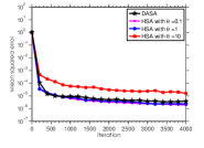
(a) Setting S$(1)$

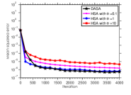
(b) Setting S$(4)$

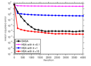
(c) Setting S$(11)$

Figure 4: The bandwidth-sharing problem – MSE – DASA vs. HSA schemes

For example, HSA scheme with $\theta=10$ performs poorly in settings S$(1)$ and S$(4)$, while it outperforms other schemes in setting S$(11)$. We also observe that changing $m_{b}$ from $1$ to $0.1$ does not affect the error. This is because the optimal solution $x^{*}$ remains feasible for a smaller vector $B$. On the other hand, the error decreases when we use $m_{b}=0.01$. Figure 5 presents the flow rates of the users in different routes for the setting $S(4)$.

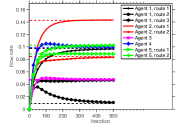
(a) DASA

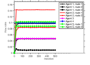
(b) HSA with $\theta=1$

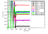
(c) HSA with $\theta=10$

Figure 5: The bandwidth-sharing problem – flow rates for the setting S$(4)$

One immediate observation is that the flow rates of HSA scheme with $\theta=10$ fluctuates noticeably in the beginning due to a very large stepsize. Figure 6 provides an image of the $90\%$ CIs for the setting $S(4)$.

(a) DASA

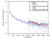
(b) HSA with $\theta=1$

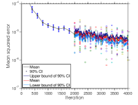
(c) HSA with $\theta=10$

Figure 6: The bandwidth-sharing problem – $90\%$ CIs for the setting S$(4)$

We used two formats to present the intervals. The left-hand side half of each plot shows the intervals with line segments, while the other half shows the lower and upper bound of the intervals continuously. The colorful points represent the $25$ sample errors at corresponding iterations. We see that the DASA scheme and HSA scheme with $\theta=1$ have CIs with similar size and a smooth mean while the mean in HSA scheme with $\theta=10$ is nonsmooth and oscillates more as the algorithm proceeds.

5.2 A networked stochastic Nash-Cournot game

Consider a networked Nash-Cournot game akin to that described in Example 1. Specifically, let firm $i$’s generation and sales decisions at node $j$ be given by $g_{ij}$ and $s_{ij}$, respectively. Suppose the price function $p_{j}$ is given by $p_{j}(\bar{s}_{j},a_{j},b_{j})=a_{j}-b_{j}\bar{s}_{j}^{\sigma}$, where $\bar{s}_{j}=\sum_{i}s_{ij}$, $\sigma\geq 1$ and $a_{j}$ and $b_{j}$ are uniformly distributed random variables defined over the intervals $[lb_{j}^{a},ub_{j}^{a}]$ and $[lb_{j}^{b},ub_{j}^{b}]$, respectively. For purposes of simplicity, we assume that the generation cost is linear and is given by $c_{ij}g_{ij}$. We also impose a bound on sales decisions, as specified $s_{ij}\leq cap_{ij}^{\prime}$ for all $i$ and $j$. Note that sales decisions are always bounded by aggregate generation capacity. The optimization model for the $i$-th firm is given by:

minimize $$\qquad\mathsf{E}\!\left[\sum_{j=1}^{M}\left(c_{ij}g_{ij}-s_{ij}(a_{j}-b_{j}\bar{s}_{j}^{\sigma})\right)\right]$$ (51)

subject to $$\qquad x_{i}=(s_{i\cdot};g_{i\cdot})\in X_{i}\triangleq\left\{\begin{aligned} &\sum_{j=1}^{M}g_{ij}=\sum_{j=1}^{M}s_{ij},\\ &g_{ij}\leq\mathrm{cap}_{ij},\quad s_{ij}\leq\mathrm{cap}_{ij}^{\prime},\qquad j=1,\ldots,M,\\ &g_{ij},s_{ij}\geq 0,\qquad j=1,\ldots,M.\end{aligned}\right\}.$$

As discussed in [15], when $1<\sigma\leq 3$ and $M\leq\frac{3\sigma-1}{\sigma-1}$, the mapping $F$ is strictly monotone and strong monotonicity can be induced using a regularized mapping, given that our interest lies in strongly monotone problems. On the other hand, when $\sigma>1$, it is difficult to check that mapping $F$ has Lipschitzian property. This motivates us to employ the distributed locally randomized SA schemes introduced in Sec. 4.3. Now, using regularization and randomized schemes, we would like to solve the VI$(X,F^{\epsilon}+\eta\bf{I})$, where $\eta>0$ is the regularization parameter and $F^{\epsilon}$ is defined by (28). As a consequence, this problem admits a unique solution denoted by $x^{*}_{\eta,\epsilon}$.

5.2.1 SA algorithms

In this experiment, we use four different SA schemes for solving VI$(X,F^{\epsilon}+\eta\bf{I})$ described in Sec. 3.2 and Sec. 4:

MSR-DASA scheme.

In this scheme, we employ the algorithm (41) and assume that the random vector $z$ is generated via the MSR scheme, i.e., $z_{i}$ is uniformly distributed on the set $B_{n_{i}}(0,\epsilon_{i})$ while the mapping $F_{\epsilon}$ is defined by (28). One immediate benefit of applying this scheme is that the Lipschitzian parameter can be estimated from Prop. 6b. Moreover, we assume that the stepsizes $\gamma_{k,i}$ are given by (26)-(27). The multiplier $r_{i}$ is randomly chosen for each firm within the prescribed range. The constant $c$ is maintained at $\frac{\eta}{4}$. Parameters $D$ and $\nu$ need to be estimated, while the Lipschitzian parameter $L$ is obtained by Prop. 6b, i.e.,

$$L=\sqrt{N}\|C\|\max_{j=1,\ldots,N}\left\{\kappa_{j}\frac{n_{j}!!}{(n_{j}-1)!!}\,\frac{1}{\epsilon_{j}}\right\}.$$

MSR-HSA schemes.

Analogous to the MSR-DASA scheme, this scheme uses the distributed locally randomized SA algorithm (41) where for any $i=1,\ldots,N$, the random vector $z_{i}$ is uniformly drawn from the ball $B_{n_{i}}(0,\epsilon_{i})$ and mapping $F_{\epsilon}$ is defined by (28). The difference is that here we use the harmonic stepsize of the form $\frac{\theta}{k}$ at $k$-th iteration for any firm, where $\theta>0$.

MCR-DASA scheme.

This scheme is similar to the MSR-DASA scheme with one key difference. We assume that random vector $z$ is generated by the MCR scheme, i.e., for any $i=1,\ldots,N$, random vector $z_{i}$ is uniformly drawn from the cube $C_{n_{i}}(0,\epsilon_{i})$ independent from any $z_{j}$ with $j\neq i$. The Lipschitz constant $L$ required for calculating the stepsizes is given by Prop. 7b:

$$L=\frac{\sqrt{n}\|C^{\prime}\|}{\min_{j=1,\ldots,N}\{\epsilon_{j}\}}.$$

MCR-HSA schemes.

This scheme uses the algorithm (41) with multi-cubic uniform random variable $z$. The stepsizes in this scheme are harmonic of the form $\frac{\theta}{k}$.

To obtain the solution $x^{*}_{\eta,\epsilon}$, we use the HSA scheme with the stepsizes $\frac{1}{k}$ using $20000$ iterations. Note that in this experiment, when we use the DASA scheme, we allow that the condition $\nu\geq\frac{DL}{\sqrt{2}}$ is violated and we replace it with $\nu\geq D$. The condition $\nu\geq D$ keeps the adaptive stepsizes positive for any $k$. As a consequence of ignoring $\nu\geq\frac{DL}{\sqrt{2}}$, the adaptive stepsizes become larger and in the order of the harmonic stepsizes in our analysis. Note that by this change, the convergence of the DASA algorithm is still guaranteed, while the result of Theorem 1d does not hold necessarily.

5.2.2 Sensitivity analysis

We consider a Nash-Cournot game with $5$ firms over a network with $3$ nodes. We set $\sigma=1.1$, $lb_{j}^{b}=0.04$, $ub_{j}^{b}=0.05$, and $lb_{j}^{a}=1$ for any $j$ and $ub^{a}=(1.5;2;2.5)$. Having these parameters fixed, our test problems are generated by changing other model’s parameters. These parameters are as follows: the parameter of locally randomized schemes $\epsilon$, the regularization parameter $\eta$, the starting point of the SA algorithm $x_{0}$, and the multiplier $M_{a}$ for the random variable $a_{j}$ for any $j$. We also consider two different settings for $\mathrm{cap}_{ij}$ and $\mathrm{cap}^{\prime}_{ij}$. Note that when $\mathrm{cap}_{ij}=1$, the constraints $s_{ij}\leq 3$ are redundant and can be removed. In our analysis we assume that $\epsilon_{i}\triangleq\epsilon$ is identical for all firms.

-	S$(i)$	$\epsilon$	$\eta$	$x_{0}$	$M_{a}$	$\mathrm{cap}_{ij}$	$\mathrm{cap}_{ij}^{\prime}$
$\epsilon$	1	0.1	0.1	$P_{1}$	$1$	$1$	$3$
	2	0.001	0.1	$P_{1}$	$1$	$1$	$3$
	3	0.0001	0.1	$P_{1}$	$1$	$1$	$3$
$\eta$	4	0.1	0.1	$P_{2}$	$1$	$10$	$1$
	5	0.1	0.05	$P_{2}$	$1$	$10$	$1$
	6	0.1	0.01	$P_{2}$	$1$	$10$	$1$
$x_{0}$	7	0.1	1	$P_{1}$	$6$	$10$	$1$
	8	0.1	1	$P_{2}$	$6$	$10$	$1$
	9	0.1	1	$P_{3}$	$6$	$10$	$1$
$M_{a}$	10	0.01	0.5	$P_{2}$	$2$	$1$	$3$
	11	0.01	0.5	$P_{2}$	$4$	$1$	$3$
	12	0.01	0.5	$P_{2}$	$6$	$1$	$3$

Table 3: The stochastic Nash-Cournot game – settings of parameters

Similar to the first experiment in Sec. 5.1.2, we consider a set of test problems corresponding to each of these parameters. In each set, one parameter changes and takes $3$ different values, while other parameters are fixed. Table 3 represents $12$ test problems as described. Note that $P_{1}$, $P_{2}$, and $P_{3}$ are three different feasible starting points. More precisely, $P_{1}=0$, $P_{2}=0.5(\mathrm{cap}^{\prime};\mathrm{cap})$, and $P_{3}=(\mathrm{cap}^{\prime};\mathrm{cap})$. Similar to the first experiment, the termination criteria is running the SA algorithms for $4000$ iterates. We run each algorithm $25$ times and then we obtain the MSE of the form $\frac{1}{25}\sum_{i=1}^{25}\|x_{k}^{i}-x^{*}_{\eta,\epsilon}\|^{2}$ for any $k=1,\ldots,4000$. Table 4 and Table 5 show the $90\%$ CIs of the error for the described schemes.

5.2.3 Results and insights

Table 4 presents the simulation results for the test problems using the MSR-DASA and MSR-HSA schemes. One observation is the effect of changing the parameter $\epsilon$ on the error of the schemes is negligible. We only see a slight change in the error of MSR-HSA scheme with $\theta=10$. Comparing the order of the error, we notice that the MSR-DASA scheme is placed second among all schemes of the first set of the test problems. In the second set, by decreasing $\eta$ the error of all the schemes, except for the MSR-HSA scheme with $\theta=0.1$, first decreases and then increases. This is not an odd observation since we used $x_{\eta,\epsilon}^{*}$ instead of $x^{*}$ to measure the errors and $x_{\eta,\epsilon}^{*}$ changes itself when $\eta$ or $\epsilon$ changes. In this set, the MSR-DASA scheme still has the second best errors among all schemes. The schemes are not much sensitive to the choice of $x_{0}$ and we observe that the second place is still reserved by the MSR-DASA scheme. Finally, in the last set, we see that increasing the factor $M_{a}$, as we expect, increases the error in most of the schemes. The reason is that increasing the order of $M_{a}$ increases both mean and variance of the random variable $a$. Importantly, we observe that our MSR-DASA scheme remains very robust among the MSR-HSA scheme.

-	S$(i)$	DASA - $90\%$ CI	HSA with $\theta=0.1$- $90\%$ CI	HSA with $\theta=1$ - $90\%$ CI	HSA with $\theta=10$ - $90\%$ CI
$\epsilon$	1	[$1.38$e${-2}$,$2.37$e${-2}$]	[$1.83$e${+1}$,$1.87$e${+1}$]	[$1.60$e${-1}$,$2.15$e${-1}$]	[$3.07$e${-3}$,$5.33$e${-3}$]
	2	[$1.38$e${-2}$,$2.37$e${-2}$]	[$1.83$e${+1}$,$1.87$e${+1}$]	[$1.60$e${-1}$,$2.15$e${-1}$]	[$3.04$e${-3}$,$5.30$e${-3}$]
	3	[$1.38$e${-2}$,$2.37$e${-2}$]	[$1.83$e${+1}$,$1.87$e${+1}$]	[$1.60$e${-1}$,$2.15$e${-1}$]	[$3.04$e${-3}$,$5.30$e${-3}$]
$\eta$	4	[$1.92$e${-3}$,$3.98$e${-3}$]	[$1.63$e${-0}$,$1.71$e${-0}$]	[$8.43$e${-3}$,$1.62$e${-2}$]	[$5.28$e${-4}$,$1.08$e${-3}$]
	5	[$1.42$e${-3}$,$3.12$e${-3}$]	[$1.84$e${-0}$,$1.93$e${-0}$]	[$7.43$e${-3}$,$1.44$e${-2}$]	[$2.59$e${-4}$,$5.76$e${-4}$]
	6	[$5.61$e${-3}$,$1.62$e${-2}$]	[$2.33$e${-0}$,$2.44$e${-0}$]	[$1.61$e${-2}$,$2.39$e${-2}$]	[$5.06$e${-4}$,$8.65$e${-4}$]
$x_{0}$	7	[$2.68$e${-6}$,$3.48$e${-6}$]	[$4.37$e${-1}$,$5.13$e${-1}$]	[$1.37$e${-6}$,$1.92$e${-6}$]	[$6.71$e${-6}$,$9.21$e${-6}$]
	8	[$2.68$e${-6}$,$3.48$e${-6}$]	[$2.22$e${-5}$,$2.91$e${-5}$]	[$1.37$e${-6}$,$1.92$e${-6}$]	[$6.71$e${-6}$,$9.21$e${-6}$]
	9	[$2.68$e${-6}$,$3.48$e${-6}$]	[$2.22$e${-5}$,$2.91$e${-5}$]	[$1.37$e${-6}$,$1.92$e${-6}$]	[$6.71$e${-6}$,$9.21$e${-6}$]
$M_{a}$	10	[$4.45$e${-3}$,$9.25$e${-3}$]	[$5.79$e${-1}$,$9.25$e${-1}$]	[$1.67$e${-3}$,$5.72$e${-3}$]	[$2.72$e${-5}$,$2.07$e${-2}$]
	11	[$8.85$e${-3}$,$1.73$e${-2}$]	[$1.25$e${-0}$,$2.12$e${-0}$]	[$9.38$e${-4}$,$1.82$e${-2}$]	[$4.52$e${-3}$,$3.22$e${-2}$]
	12	[$1.92$e${-2}$,$3.91$e${-2}$]	[$8.51$e${-1}$,$2.31$e${-0}$]	[$1.87$e${-3}$,$4.15$e${-2}$]	[$1.04$e${-2}$,$7.23$e${-2}$]

Table 4: The stochastic Nash-Cournot game – $90\%$ CIs for MSR-DASA and MSR-HSA schemes

Table 5 shows the error estimations using the MCR-DASA and MCR-HSA schemes. Comparing these results with the MSR schemes in Table 4, we see that the sensitivity of the MCR schemes to the parameters is very similar to that of MSR schemes and the MCR-DASA scheme performs as the second best among all MCR schemes. We also see that in most of the settings, the error of the MSR-DASA scheme is slightly smaller than the error of the MCR-DASA scheme. One reason can be that the MSR scheme has a smaller Lipschitz constant than the MCR scheme for our problem settings.

-	S$(i)$	DASA - $90\%$ CI	HSA with $\theta=0.1$- $90\%$ CI	HSA with $\theta=1$ - $90\%$ CI	HSA with $\theta=10$ - $90\%$ CI
$\epsilon$	1	[$1.22$e${-2}$,$2.55$e${-2}$]	[$1.84$e${+1}$,$1.88$e${+1}$]	[$1.78$e${-1}$,$2.29$e${-1}$]	[$2.42$e${-3}$,$4.21$e${-3}$]
	2	[$1.21$e${-2}$,$2.53$e${-2}$]	[$1.84$e${+1}$,$1.88$e${+1}$]	[$1.78$e${-1}$,$2.28$e${-1}$]	[$2.37$e${-3}$,$4.13$e${-3}$]
	3	[$1.21$e${-2}$,$2.53$e${-2}$]	[$1.84$e${+1}$,$1.88$e${+1}$]	[$1.78$e${-1}$,$2.28$e${-1}$]	[$2.37$e${-3}$,$4.13$e${-3}$]
$\eta$	4	[$4.17$e${-3}$,$9.50$e${-3}$]	[$1.65$e${-0}$,$1.74$e${-0}$]	[$9.37$e${-3}$,$1.84$e${-2}$]	[$7.38$e${-4}$,$1.73$e${-3}$]
	5	[$1.41$e${-3}$,$4.06$e${-3}$]	[$1.85$e${-0}$,$1.93$e${-0}$]	[$6.88$e${-3}$,$1.32$e${-2}$]	[$2.85$e${-4}$,$5.06$e${-4}$]
	6	[$8.19$e${-3}$,$1.88$e${-2}$]	[$2.37$e${-0}$,$2.46$e${-0}$]	[$1.85$e${-2}$,$3.10$e${-2}$]	[$4.18$e${-4}$,$7.05$e${-4}$]
$x_{0}$	7	[$2.25$e${-5}$,$2.88$e${-5}$]	[$4.31$e${-1}$,$5.12$e${-1}$]	[$9.41$e${-6}$,$1.18$e${-5}$]	[$3.99$e${-5}$,$5.27$e${-5}$]
	8	[$2.25$e${-5}$,$2.88$e${-5}$]	[$1.13$e${-4}$,$1.58$e${-4}$]	[$9.40$e${-6}$,$1.18$e${-6}$]	[$3.99$e${-5}$,$5.27$e${-5}$]
	9	[$2.25$e${-5}$,$2.88$e${-5}$]	[$1.13$e${-4}$,$1.58$e${-4}$]	[$9.40$e${-6}$,$1.18$e${-5}$]	[$3.99$e${-5}$,$5.27$e${-5}$]
$M_{a}$	10	[$1.66$e${-3}$,$4.29$e${-3}$]	[$6.17$e${-1}$,$8.88$e${-1}$]	[$4.21$e${-4}$,$1.79$e${-3}$]	[$3.82$e${-4}$,$8.30$e${-3}$]
	11	[$3.03$e${-3}$,$1.22$e${-2}$]	[$1.29$e${-0}$,$2.23$e${-0}$]	[$9.63$e${-4}$,$5.77$e${-3}$]	[$2.48$e${-3}$,$2.52$e${-2}$]
	12	[$6.05$e${-3}$,$2.60$e${-2}$]	[$8.50$e${-1}$,$2.49$e${-0}$]	[$2.27$e${-3}$,$1.29$e${-2}$]	[$5.54$e${-3}$,$5.67$e${-2}$]

Table 5: The stochastic Nash-Cournot game – $90\%$ CIs for MCR-DASA and MCR-HSA schemes

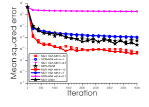
(a) Setting S$(5)$

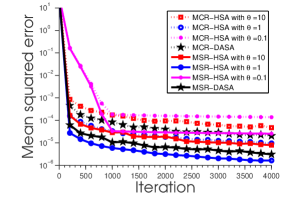
(b) Setting S$(8)$

Figure 7: The stochastic Nash-Cournot game – comparison among all the schemes

Figure 7 illustrates a comparison among the different schemes described in Sec. 5.2.1 for the case of setting S$(5)$ and S$(8)$. All the MSR schemes are shown with solid lines, while the MCR schemes are presented with dashed lines. There are some immediate observations here. Regarding the order of the error, in both if the settings S$(5)$ and S$(8)$, the schemes with the distributed adaptive stepsizes given by (26)-(27) are the second best scheme among each of MSR and MCR schemes. This indicates the robustness of the DASA scheme compared with the HSA schemes. We also observe that in the setting S$(5)$, the HSA schemes with $\theta=10$ (both MSR and MCR) have the minimum error, while in setting S$(8)$, the HSA schemes with $\theta=1$ has the minimum error. This is an illustration of sensitivity of HSA schemes to the setting of problem parameters. Let us now compare the MSR schemes with the MCR schemes. In the setting S$(5)$, the MSR and MCR schemes perform very closely and in fact, it is hard to distinguish the difference between their errors. On the other hand, in the setting S$(8)$, we see that the MSR schemes have a better performance than their MCR counterparts.

(a) MSR-DASA scheme

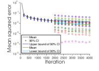
(b) MSR-HSA scheme with $\theta=1$

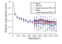
(c) MSR-HSA scheme with $\theta=10$

Figure 8: The stochastic Nash-Cournot game – setting S$(5)$ – MSR-DASA vs. MSR-HSA schemes

Figure 8 illustrates the $90\%$ confindence intervals for the MSR schemes with the setting S$(5)$. Teese intervals are shown with line segments in the left-hand side half of each plot and shown with continious bouns in the right-hand side half. The colourful points present the samples at each level of iterates. Impostantly, we observe that the CIs of MSR-DASA scheme are as tight as the MSR-HSA scheme with $\theta=1$ and they are tighter than the ones in the MSR-HSA scheme with $\theta=10$. Figure 9 shows the similar comparison for the MCR schemes.

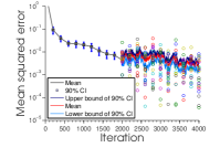
(a) MCR-DASA scheme

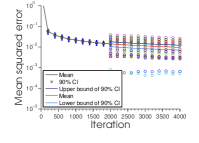
(b) MCR-HSA scheme with $\theta=1$

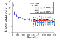
(c) MCR-HSA scheme with $\theta=10$

Figure 9: The stochastic Nash-Cournot game – setting S$(5)$ – MCR-DASA vs. MCR-HSA schemes

6 Concluding remarks

We consider the solution of strongly monotone Cartesian stochastic variational inequality problems through stochastic approximation (SA) schemes. Motivated by the naive stepsize rules employed in most SA implementations, we develop a recursive rule that adapts to problem parameters such as the Lipschitz and monotonicity constants of the map and ensures almost-sure convergence of the iterates to the unique solution. An extension to the distributed multi-agent regime is provided. A shortcoming of this approach is the reliance on the availability of a Lipschitz constant. This motivates the construction of two locally randomized techniques to cope with instances where the mapping is either not Lipschitz or estimating the parameter is challenging. In each of these techniques, we show that an approximation of the original mapping is Lipschitz continuous with a prescribed constant. We utilize these techniques in developing a distributed locally randomized adaptive steplength SA scheme where we perturb the mapping at each iteration by a uniform random variable over a prescribed distribution. It is shown that this scheme produces iterates that converge to a solution of an approximate problem, and the sequence of approximate solutions converge to the unique solution of the original stochastic variational problem. In Sec. 5, we apply our schemes on two sets of problems, a bandwidth-sharing problem in communication networks and a networked stochastic Nash-Cournot game. Through these examples, we observed that the adaptive distributed stepsize scheme displays far more robustness than the standard implementations that leverage harmonic stepsizes of the form $\frac{\theta}{k}$ in both problems. Furthermore, the randomized smoothing techniques assume utility in the Cournot regime where Lipschitz constants cannot be easily derived.

References

• [1] T. Alpcan and T. Başar, A game-theoretic framework for congestion control in general topology networks, in Proceedings of the 41st IEEE Conference on Decision and Control, December 2002, pp. 1218– – 1224.
• [2]  , Distributed algorithms for Nash equilibria of flow control games, in Advances in Dynamic Games, vol. 7 of Annals of the International Society of Dynamic Games, Birkhäuser Boston, 2003, pp. 473–498.
• [3] D. P. Bertsekas, Stochastic optimization problems with nondifferentiable functionals with an application in stochastic programming, in Proceedings of 1972 IEEE Conference on Decision and Control, 1972, pp. 555–559.
• [4] V. S. Borkar, Stochastic Approximation: A Dynamical Systems Viewpoint, Cambridge University Press, 2008.
• [5] R. H. Byrd, M. E. Hribar, and J. Nocedal, An interior point algorithm for large-scale nonlinear programming, SIAM Journal on Optimization, 9 (1999), pp. 877 –900.
• [6] S.-W. Cho and A. Goel, Bandwidth allocation in networks: a single dual update subroutine for multiple objectives, Combinatorial and algorithmic aspects of networking, 3405 (2005), pp. 28–41.
• [7] D. Cicek, M. Broadie, and A. Zeevi, General bounds and finite-time performance improvement for the kiefer-wolfowitz stochastic approximation algorithm, To appear in Operations Research, (2011).
• [8] Y. M. Ermoliev, Stochastic Programming Methods, Nauka, Moscow, 1976.
• [9]  , Stochastic quasigradient methods, in Numerical Techniques for Stochastic Optimization, Sringer-Verlag, 1983, pp. 141–185.
• [10]  , Stochastic quasigradient methods and their application to system optimization, Stochastics, 9 (1983), pp. 1–36.
• [11] F. Facchinei and J.-S. Pang, Finite-dimensional variational inequalities and complementarity problems. Vols. I,II, Springer Series in Operations Research, Springer-Verlag, New York, 2003.
• [12] A. P. George and W. B. Powell, Adaptive stepsizes for recursive estimation with applications in approximate dynamic programming, Machine Learning, 65 (2006), pp. 167–198.
• [13] A. M. Gupal, Stochastic methods for solving nonsmooth extremal problems (Russian), Naukova Dumka, 1979.
• [14] H. Jiang and H. Xu, Stochastic approximation approaches to the stochastic variational inequality problem, IEEE Transactions on Automatic Control, 53 (2008), pp. 1462–1475.
• [15] A. Kannan and U. V. Shanbhag, Distributed computation of equilibria in monotone Nash games via iterative regularization techniques, SIAM Journal of Optimization, 22 (2012), pp. 1177–1205.
• [16] A. Kannan, U. V. Shanbhag, and H. . M. Kim, Addressing supply-side risk in uncertain power markets: stochastic Nash models, scalable algorithms and error analysis, Optimization Methods and Software (online first), 0 (2012), pp. 1–44.
• [17] A. Kannan, U. V. Shanbhag, and H. M. Kim, Strategic behavior in power markets under uncertainty, Energy Systems, 2 (2011), pp. 115–141.
• [18] F. Kelly, A. Maulloo, and D. Tan, Rate control for communication networks: shadow prices, proportional fairness, and stability, Journal of the Operational Research Society, 49 (1998), pp. 237–252.
• [19] J. Koshal, A. Nedić, and U. V. Shanbhag, Single timescale regularized stochastic approximation schemes for monotone nash games under uncertainty, Proceedings of the IEEE Conference on Decision and Control (CDC), (2010), pp. 231–236.
• [20] J. Koshal, A. Nedić, and U. V. Shanbhag, Single timescale stochastic approximation for stochastic nash games in cognitive radio systems, 2011, pp. 1–8.
• [21] H. J. Kushner and G. G. Yin, Stochastic Approximation and Recursive Algorithms and Applications, Springer New York, 2003.
• [22] H. Lakshmanan and D. Farias, Decentralized resource allocation in dynamic networks of agents, SIAM Journal on Optimization, 19 (2008), pp. 911–940.
• [23] J. Linderoth, A. Shapiro, and S. Wright, The empirical behavior of sampling methods for stochastic programming, Ann. Oper. Res., 142 (2006), pp. 215–241.
• [24] C. Metzler, B. Hobbs, and J.-S. Pang, Nash-cournot equilibria in power markets on a linearized dc network with arbitrage: Formulations and properties, Networks and Spatial Theory, 3 (2003), pp. 123–150.
• [25] V. I. Norkin, The analysis and optimization of probability functions, tech. rep., International Institute for Applied Systems Analysis technical report, 1993. WP-93-6.
• [26] B. Polyak, Introduction to optimization, Optimization Software, Inc., New York, 1987.
• [27] W. B. Powell, Approximate Dynamic Programming: Solving the Curses of Dimensionality, John Wiley $\&$ Sons, Inc., Hoboken, New Jersey, 2010.
• [28] H. Robbins and S. Monro, A stochastic approximation method, Ann. Math. Statistics, 22 (1951), pp. 400–407.
• [29] G. Scutari, F. Facchinei, J.-S. Pang, and D. Palomar, Monotone games for cognitive radio systems, (2012), pp. 83–112.
• [30] G. Scutari and D. P. Palomar, Mimo cognitive radio: a game theoretical approach, IEEE Transactions on Signal Processing, 58 (2010), pp. 761–780.
• [31] S. Shakkottai and R. Srikant, Network optimization and control, Foundations and Trends in Networking, 2 (2007), pp. 271–379.
• [32] U. V. Shanbhag, G. Infanger, and P. Glynn, A complementarity framework for forward contracting under uncertainty, Operations Research, 59 (2011), pp. 810–834.
• [33] A. Shapiro, Monte Carlo sampling methods, in Handbook in Operations Research and Management Science, vol. 10, Elsevier Science, Amsterdam, 2003, pp. 353–426.
• [34] J. C. Spall, Introduction to Stochastic Search and Optimization: Estimation, Simulation, and Control, Wiley, Hoboken, NJ, 2003.
• [35] R. Srikant, Mathematics of Internet Congestion Control, Birkhauser, 2004.
• [36] V. A. Steklov, Sur les expressions asymptotiques decertaines fonctions définies par les équations différentielles du second ordre et leers applications au problème du dévelopement d’une fonction arbitraire en séries procédant suivant les diverses fonctions, Comm. Charkov Math. Soc., 2 (1907), pp. 97–199.
• [37]  , Main Problems of Mathematical Physics, Nauka, Moscow, 1983.
• [38] J. Wang, G. Scutari, and D. P. Palomar, Robust mimo cognitive radio via game theory, IEEE Transactions on Signal Processing, 59 (2011), pp. 1183–1201.
• [39] H. Yin, U. V. Shanbhag, and P. G. Mehta, Nash equilibrium problems with scaled congestion costs and shared constraints, IEEE Transactions of Automatic Control, 56 (2009), pp. 1702–1708.
• [40] F. Yousefian, A. Nedić, and U. Shanbhag, A regularized adaptive steplength stochastic approximation scheme for monotone stochastic variational inequalities, Proceedings of the 2011 Winter Simulation Conference, (2011), pp. 4110–4121.
• [41] F. Yousefian, A. Nedić, and U. V. Shanbhag, On stochastic gradient and subgradient methods with adaptive steplength sequences, Automatica, 48 (2012), pp. 56–67. An extended version of the paper available at: http://arxiv.org/abs/1105.4549.