Causal graph-based video segmentation

Abstract

Numerous approaches in image processing and computer vision are making use of super-pixels as a pre-processing step. Among the different methods producing such over-segmentation of an image, the graph-based approach of Felzenszwalb and Huttenlocher is broadly employed. One of its interesting properties is that the regions are computed in a greedy manner in quasi-linear time. The algorithm may be trivially extended to video segmentation by considering a video as a 3D volume, however, this can not be the case for causal segmentation, when subsequent frames are unknown. We propose an efficient video segmentation approach that computes temporally consistent pixels in a causal manner, filling the need for causal and real time applications.

1 Introduction

A segmentation of video into consistent spatio-temporal segments is a largely unsolved problem. While there have been attempts at video segmentation, most methods are non causal and non real-time. This paper proposes a fast method for real time video segmentation, including semantic segmentation as an application.

An large number of approaches in computer vision makes use of super-pixels at some point in the process. For example, semantic segmentation [5], geometric context indentification [10], extraction of support relations between object in scenes [14], etc. Among the most popular approach for super-pixel segmentation, two types of methods are distinguishable. Regular shape super-pixels may be produced using normalized cuts [16] for instance. More object – or part of object – shaped super-pixels can be generated from watershed based approaches. In particular the method of Felzenswalb and Huttenlocher [6] produces such results.

It is a real challenge to obtain a decent delineation of objects from a single image. When it comes to real-time data analysis, the problem is even more difficult. However, additional cues can be used to constrain the solution to be temporally consistent, thus helping to achieve better results. Since many of the underlying algorithms are in general super-linear, there is often a need to reduce the dimensionality of the video. To this end, developing low level vision methods for video segmentation is necessary. Currently, most video processing approaches are non-causal, that is to say, they make use of future frames to segment a given frame, sometimes requiring the entire video [9]. This prevents their use for real-time applications.

Some approaches have been designed to address the causal video segmentation problem [15, 13]. [15] makes use of the mean shift method [2]. As this method works in a feature space, it does not necessary cluster spatially consistent super-pixels. A more recent approach, specifically applied for semantic segmentation, is the one of Miksik et al. [13]. The work of [13] is employing an optical flow method to enforce the temporal consistency of the semantic segmentation. Our approach is different because it aims to produce super-pixels, and possibly uses the produced super-pixels for smoothing semantic segmentation results. Furthermore, we do not use any optical flow pre-computation that would prevent us having real time performances on a CPU.

Some works use the idea of enforcing some consistency between different segmentations [7, 12, 11, 8]. [7] formulates a co-clustering problem as a Quadratic Semi-Assignment Problem. However solving the problem for a pair of images takes about a minute. Alternatively, [12] and [8] identify the corresponding regions using graph matching techniques. The approach of [8] is only illustrated on very coarse image segmentation, and the graph matching is performed between graphs that contain a dozen of regions. In both cases, the number of tracked regions is limited in the experiments to a small amount.

The idea developped in this paper is to perform independent segmentations and match the produced super-pixels to define markers. The markers are then used to produce the final segmentation by minimizing a global criterion defined on the image. The graph used in the independent segmentation part is reused in the final segmentation stage, leading thus to gains in speed, and real-time performances on a single core CPU.

2 Method

Given a segmentation $S_{t}$ of an image at time $t$, we wish to compute a segmentation $S_{t+1}$ of the image at time $t+1$ which is consistent with the segments of the result at time $t$.

2.1 Independent image segmentation

The super-pixels produced by [6] have been shown to satisfy the global properties of being not too coarse and not too fine according to a particular region comparison function. In order to generate superpixels close to the ones produced by [6], we first generate independent segmentations of the 2D images using [6]. We name these segmentations $S^{\prime}_{1},...,S^{\prime}_{t}$. The principle of segmentation is fairly simple. We define a graph $G_{t}$, where the nodes correspond to the image pixels, and the edges link neighboring nodes in 8-connectivity. The edge weights $\omega_{ij}$ between nodes $i$ and $j$ are given by a color gradient of the image.

A Minimum Spanning Tree (MST) is build on $G_{t}$, and a region merging criteria is defined. Specifically, two regions $X$ and $Y$ are merged when:

$$Diff(X,Y)\leq\min\left(Int(X)+\frac{k}{|X|},Int(Y)+\frac{k}{|Y|}\right),$$ (1)

where $k$ is a parameter allowing to prevent the merging of large regions. The internal difference $Int(X)$ of a region $X$ is the highest weight of an edge linking two vertices of $X$ in the MST. The difference $Diff(X,Y)$ between two neighboring regions $X$ and $Y$ is the smallest weight of an edge that links $X$ to $Y$.

Once an image is independently segmented, resulting in $S^{\prime}_{t+1}$, we then face the question of the propagation of the temporal consistency given the non overlapping contours of $S_{t}$ and $S^{\prime}_{t+1}$.

Our solution is the development of a cheap graph matching technique to obtain correspondences between segments from $S_{t}$ and these of $S^{\prime}_{t+1}$. This first step is described in Section 2.2. We then mine these correspondences to create markers (also called seeds) to compute the final labeling $S_{t+1}$ by solving a global optimization problem. This second step is detailed in Section 2.3.

2.2 Graph matching procedure

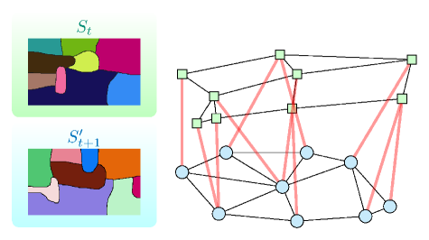
Figure 1: Illustration of the graph matching procedure

The basic idea is to use the segmentation $S_{t}$ and segmentation $S^{\prime}_{t+1}$ to produce markers before a final segmentation of image at time $t+1$. Therefore, in the process of computing a new segmentation $S_{t+1}$, a graph $G$ is defined. The vertices of $G$ comprises to two sets of vertices: $V_{t}$ that corresponds to the set of regions of $S_{t}$ and $V^{\prime}_{t+1}$ that corresponds to the set of regions of $S^{\prime}_{t+1}$. Edges link regions characterised by a small distance between their centroids. The edges weights between vertex $i\in V_{t}$ and $j\in V^{\prime}_{t+1}$ are given by a similarity measure taking into account distance and differences between shape and appearance

$$w_{ij}=\frac{(|r_{i}|+|r_{j}|)d(c_{i},c_{j})}{|r_{i}\cap r_{j}|}+a_{ij},$$ (2)

where $|r_{i}|$ denotes the number of pixels of region $r_{i}$, $|r_{i}\cap~{}r_{j}|$ the number of pixels present in $r_{i}$ and $r_{j}$ with aligned centroids, and $a_{ij}$ the appearance difference of regions $r_{i}$ and $r_{j}$. In our experiments $a_{ij}$ was defined as the difference between mean color intensities of the regions.

The graph matching procedure is illustrated in Figure 1 and produces the following result: For each region of $S^{\prime}_{t+1}$, its best corresponding region in image $S_{t}$ is identified. More specifically, each node $i$ of $V_{t}$ is associated with the node $j$ of $V^{\prime}_{t+1}$ which minimizes $w_{ij}$. Symmetrically, for each region of $S_{t}$, its best corresponding region in image $S^{\prime}_{t+1}$ is identified, that is to say each node $i$ of $V^{\prime}_{t+1}$ is associated with the node $j$ of $V_{t}$ which minimizes $w_{ij}$.

2.3 Final segmentation procedure

The final segmentation $S_{t+1}$ is computed using a minimum spanning forest procedure. This seeded segmentation algorithm that produces watershed cuts [4] is strongly linked to global energy optimization methods such as graph-cuts [1, 3] as detailed in Section 2.4. In addition to theoretical guaranties of optimality, this choice of algorithm is motivated by the opportunity to reuse the sorting of edges that is performed in 2.1 and constitutes the main computational effort. Consequently, we reuse here the graph $G_{t+1}(V,E)$ built for the production of independent segmentation $S^{\prime}_{t+1}$.

Data: A weighted graph $G(V,E)$ and a set of labeled nodes makers $L$. Nodes of $V\setminus L$ have unknown labels initially.

Result: A labeling $x$ associating a label to each vertex.

Sort the edges of $E$ by increasing order of weight.

while any node has an unknown label do  Find the edge $e_{ij}$ in $E$ of minimal weight;

if $v_{i}$ or $v_{j}$ have unknown label values then  Merge $v_{i}$ and $v_{j}$ into a single node, such that when the value for this merged node becomes known, all merged nodes are assigned the same value of $x$ and considered known.    

Algorithm 1 Minimum Spanning Forest algorithm

The minimum spanning forest algorithm is recalled in Algorithm 1. The seeds, or markers, are defined using the regions correspondences computed in the previous section, according to the procedure detailed below. For each segment $s^{\prime}$ of $S^{\prime}_{t+1}$ four cases may appear:

1. $s^{\prime}$ has one and only one matching region $s$ in $S_{t}$: propagate the label $l_{s}$ of region $s$. All nodes of $s^{\prime}$ are labeled with the label $l_{s}$ of region $s$.

2. $s^{\prime}$ has several corresponding regions $s_{1},...,s_{r}$: propagate seeds from $S_{t}$. The coordinates of regions $s_{1},...,s_{r}$ are centered on region $s^{\prime}$. The labels of regions $s_{1},...,s_{r}$ whose coordinates are in the range of $s^{\prime}$ are propagated to the nodes of $s^{\prime}$.

3. $s^{\prime}$ has no matching region : The region is labeled by the label $l_{s}^{\prime}$ itself.

4. If none of the previous cases is fulfilled, it means that $s^{\prime}$ is part of a larger region $s$ in $S_{t}$. If the size of $s^{\prime}$ is small, a new label is created. Otherwise, the label $l_{s}$ is propagated in $s^{\prime}$ as in case 1.

Before applying the minimum spanning forest algorithm, a safety test is performed to check that the map of produced markers does not differ two much from the segmentation $S^{\prime}_{t+1}$. If the test shows large differences, an eroded map of $S^{\prime}_{t+1}$ is used to correct the markers.

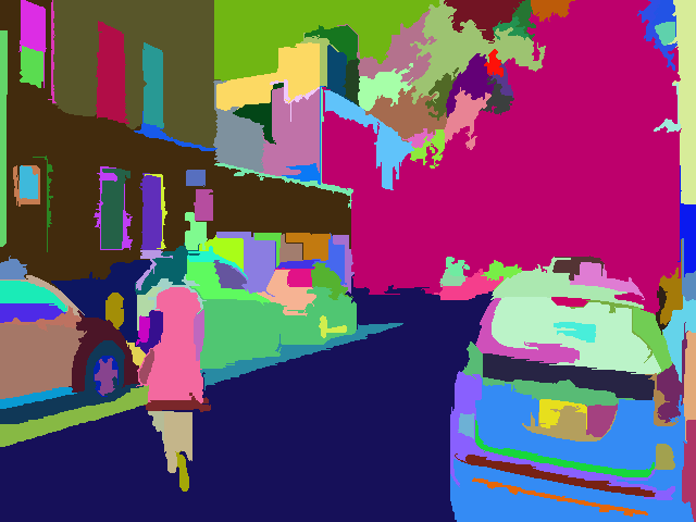
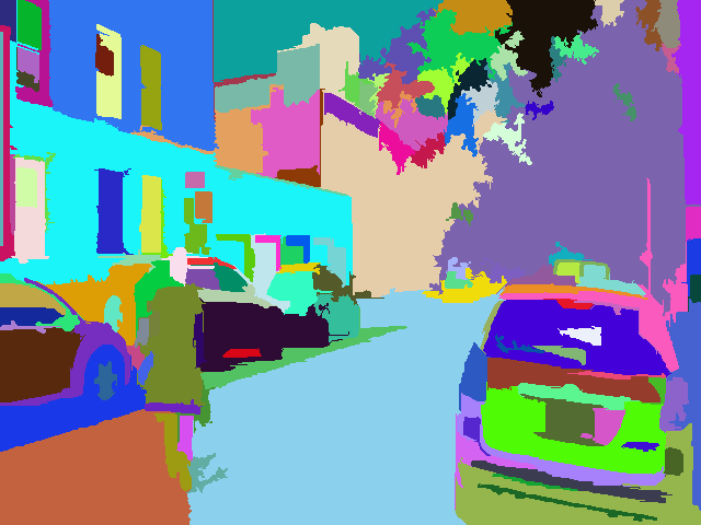
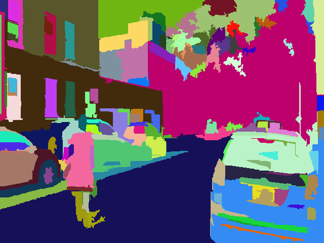
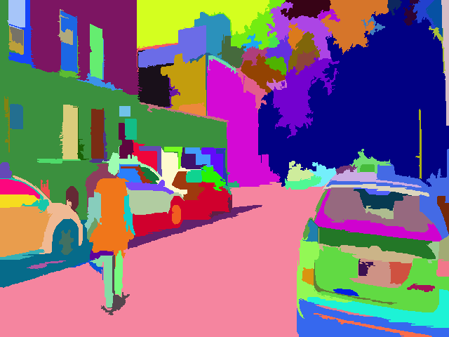
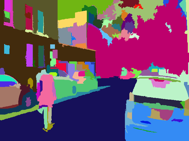
Independent segmentations	Temporally consistent segm-
$S^{\prime}_{1},S^{\prime}_{2}$ and $S^{\prime}_{3}$	entations $S_{1}(=S^{\prime}_{1}),S_{2}$, and $S_{3}$

Figure 2: Segmentation results on 3 consecutive frames of the NYU-Scene dataset.

2.4 Global optimization guaranties

Several graph-based segmentation problems, including minimum spanning forests, graph cuts, random walks and shortest paths have recently been shown to belong to a common energy minimization framework [3]. The considered problem is to find a labeling $x^{*}\in\mathbb{R}^{|V|}$ defined on the nodes of a graph that minimizes

$$\begin{gathered}E(x)=\sum_{e_{ij}\in E}w_{ij}^{p}|x_{j}-x_{i}|^{q}+\sum_{v_{i}\in V}w_{i}^{p}|l_{i}-x_{i}|^{q},\end{gathered}$$ (4)

where $l$ represents a given configuration and $x$ represents the target configuration. The result of $\lim_{p\rightarrow\infty}\operatorname*{arg\,min}_{x}E(x)$ for values of $q\geq 1$ always produces a cut by maximum (equivalently minimum) spanning forest. The reciprocal is also true if the weights of the graph are all different.

In the case of our application, the pairwise weights $w_{ij}$ is given by an inverse function of the original weights $\omega_{ij}$. The pairwise term thus penalizes any unwanted high-frequency content in $x$ and essentially forces $x$ to vary smoothly within an object, while allowing large changes across the object boundaries. The second term enforces fidelity of $x$ to a specified configuration $l$, $w_{i}$ being the unary weights enforcing that fidelity.

The enforcement of markers $l_{s}$ as hard constrained may be viewed as follows: A node of label $l_{s}$ is added to the graph, and linked to all nodes $i$ of $V$ that are supposed to be marked. The unary weights $\omega_{i,l_{s}}$ are set to arbitrary large values in order to impose the markers.

Figure 3: Comparison with the mean-shift segmentation method of Paris [15] on Frame 19 and 20. $k=200,\delta=400,\sigma=0.5$.

2.5 Applications to optical flow and semantic segmentation

An optical flow map may be easily estimated from two successive segmentations $S_{t}$ and $S_{t+1}$. For each region $r$ of $S_{t+1}$, if the label of $r$ comes from a label present in a region $s$ of the segmentation $S_{t}$, the optical flow in $r$ is computed as the distance between the centroid of $r$ and the centroid of $s$. The optical flow map may be used as a sanity check for region tracking applications. By principle, a video sequence will not contain displacements of objects greater than a certain value.

For each superpixel $s$ of $S_{t+1}$, if the label of region $s$ comes from the previous segmentation $S_{t}$, then the semantic prediction from $S_{t}$ is propagated to $S_{t+1}$. Otherwise, in case the label of $s$ is a new label, the semantic prediction is computed using the prediction at time $t+1$. As some errors may appear in the regions tracking, the labels of regions that have inconsistent large values in optical flow maps are not propagated.

For the specific task of semantic segmentation, results can be improved by exploiting the contours of the recognized objects. Semantic contours such as for example transition between a building and a tree for instance, might not be present in the gradient of the raw image. Thus, in addition to the pairwise weights $\omega$ described in Section 2.1, we add a constant in the presence of a semantic contour.

3 Results

We now demonstrate the efficiency and versatility of our approach by applying it to different problems: simple super-pixel segmentation, semantic scene labeling, and optical flow.

Following the implementation of [6], we pre-process the images using a Gaussian filtering step with a kernel of variance $\sigma$ is employed. A post-processing step that removes regions of small size, that is to say below a threshold $\delta$ is also performed. As in [6], we denote the scale of observation parameter by $k$.

3.1 Super-pixel segmentation

Experiments are performed on two different types of videos: videos where the camera is static, and videos where the camera is moving. The robustness of our approach to large variations in the region sizes and large movements of camera is illustrated on Figure 2.

A comparison with the temporal mean shift segmentation of Paris [15] is displayed at Figure 3. The super-pixels produced by the [15] are not spatially consistent as the segmentation is performed in the feature (color) space in their case. Our approach is slower, although qualified for real-time application but computes only spatially consistent super-pixels.

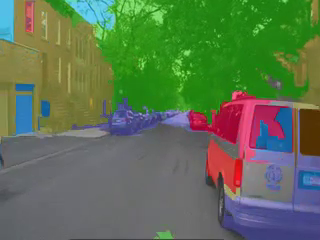
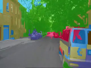
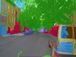
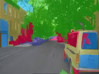
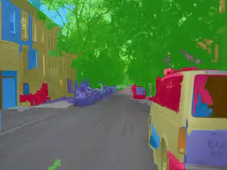
(a) Independent segmentations with no temporal smoothing

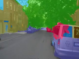
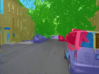
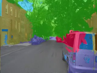
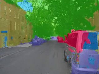
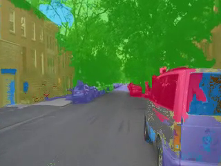
(b) Result using the temporal smoothing method of [13]

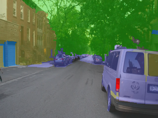
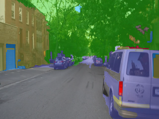
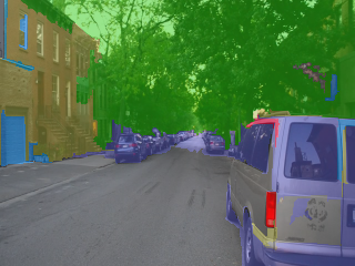
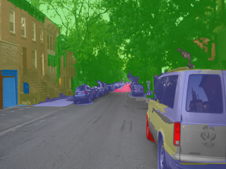
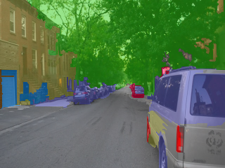
(c) Our temporally consistent segmentation

Legend: awning

balcony building

car door

person road

sidewalk sun

tree window

Figure 4: Comparison with the temporal smoothing method of [13]. Parameters used: $k=1200,\delta=100,\sigma=1.2$.

3.2 Semantic scene labeling

We suppose that we are given a noisy semantic labeling for each frame. In this work we used the semantic predictions of [5].

We compare our results with the results of [13] on the NYU-Scene dataset. The dataset consists in a video sequence of 73 frames provided with a dense semantic labeling and ground truths. The provided dense labeling being performed with no temporal exploitation, it suffers from sudden large object appearances and disappearances. As illustrated in Figure 4 our approach reduces this effect, and improves the classification performance of more than 5% as reported in Table 1. We also display results on another video in Figure (5).

	Frame	Miksik	Our
	by frame	et al.[13]	method
Accuracy	71.11	75.31	76.27
#Frames/sec		$1.33^{*}$	10.5

Table 1: Overall pixel accuracy ($\%$) for the semantic segmentation task on the NYU Scene video. ^∗Note that the reported timing does not take into account the optical flow computation needed by [13].

3.3 Optical flow

As detailed in Section 2.5, we compute the optical flow maps between subsequent frames of videos. An example of result is shown in Figure 5, that illustrates the accurate detection of a large move of the camera from the Frames 9 to 10 of a video taken on a highway.

3.4 Computation time

The experiments were performed on a laptop with 2.3 GHz intel core i7-3615QM, Memory 8Go DDR3 1600 MHz. Our method is implemented on CPU only, in C/C++, and makes use of only one core of the processor. Super-pixel segmentations take 0.1 seconds per image of size $320\times 240$ and 0.4 seconds per image of size $640\times 380$, thus demonstrating the scalability of the pipeline. All computations are included in the reported timings.

The timings of the temporal smoothing method of Miksik et al.[13] are reported in Table 1. We note that the processor used for the reported timings of [13] has similar characteristics as ours. Furthermore, Mistik et al. use an optical flow procedure that takes only 0.02 seconds per frame when implemented on GPU, but takes seconds on CPU. Our approach is thus more adapted to real time applications for instance on embedded devices where a GPU is often not available.

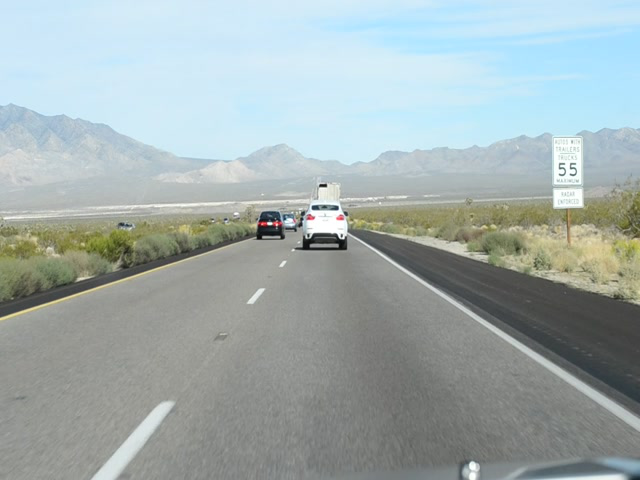
(a) Frame 9

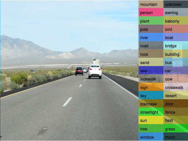
(b) Frame 10

(c) Segmentation $S_{9}$

(d) Segmentation $S_{10}$

(e) Optical flow

(f) Legend

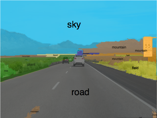
(g) Frame by frame segm.

(h) Our semantic segm.

Figure 5: By matching regions, our method can be used to derive an optical flow (e). Parameters used: $k=200,\delta=400,\sigma=0.81$

4 Conclusion

The proposed approach employs a graph matching technique to produce markers used in a global optimization procedure for video segmentation. Unlike many video segmentation techniques, our algorithm is causal – which is a required property for real-time applications – and does not require any computation of optical flow. Our experiments on challenging videos show that the obtained super-pixels are robust to large camera or objects displacement. Their use in semantic segmentation applications demonstrate that significant gains can be achieved and lead to state-of-the-art results. Furthermore, by being 8 times faster than the competing method for temporal smoothing of semantic segmentation, and up to 25 times faster if the use of GPU is not available, the proposed approach has by itself a practical interest.

References

- [1] C. Allène, J.-Y. Audibert, M. Couprie, and R. Keriven. Some links between extremum spanning forests, watersheds and min-cuts. Image and Vision Computing, 28(10):1460–1471, 2010.
- [2] D. Comaniciu, P. Meer, and S. Member. Mean shift: A robust approach toward feature space analysis. IEEE Transactions on Pattern Analysis and Machine Intelligence, 24:603–619, 2002.
- [3] C. Couprie, L. J. Grady, L. Najman, and H. Talbot. Power watershed: A unifying graph-based optimization framework. IEEE Trans. on Pattern Analysis and Machine Intelligence, 33(7):1384–1399, 2011.
- [4] J. Cousty, G. Bertrand, L. Najman, and M. Couprie. Watershed cuts: Minimum spanning forests and the drop of water principle. IEEE Trans. Pattern Analysis and Machine Intelligence, 31(8):1362–1374, 2009.
- [5] C. Farabet, C. Couprie, L. Najman, and Y. LeCun. Learning hierarchical features for scene labeling. IEEE Trans. on Pattern Analysis and Machine Intelligence, 2013. in press.
- [6] P. F. Felzenszwalb and D. P. Huttenlocher. Efficient graph-based image segmentation. International Journal of Computer Vision, 59(2):167–181, 2004.
- [7] D. Glasner, S. N. Vitaladevuni, and R. Basri. Contour-based joint clustering of multiple segmentations. In Proc. of IEEE Computer Vision and Pattern Recognition (CVPR 2011), pages 2385–2392, Washington, DC, USA, 2011.
- [8] C. Gomila and F. Meyer. Graph-based object tracking. In Proc. of IEEE International Conference on Image Processing (ICIP 2003), volume 2, pages II – 41–4 vol.3, sept. 2003.
- [9] M. Grundmann, V. Kwatra, M. Han, and I. Essa. Efficient hierarchical graph-based video segmentation. In Proc. of IEEE Computer Vision and Pattern Recognition (CVPR 2010), 2010.
- [10] D. Hoiem, A. Efros, and M. Hebert. Geometric context from a single image. In IEEE International Conference on Computer Vision (ICCV 2005), volume 1, pages 654 – 661 Vol. 1, oct. 2005.
- [11] A. Joulin, F. Bach, and J. Ponce. Multi-class cosegmentation. In Proc. of IEEE Computer Vision and Pattern Recognition (CVPR 2012), Providence, RI, USA, pages 542–549, 2012.
- [12] J. Lee, J.-H. Oh, and S. Hwang. Clustering of video objects by graph matching. In Proc. of the IEEE International Conference on Multimedia and Expo, ICME 2005, July 6-9, 2005, Amsterdam, The Netherlands, pages 394–397, 2005.
- [13] O. Miksik, D. Munoz, J. A. D. Bagnell, and M. Hebert. Efficient temporal consistency for streaming video scene analysis. Technical Report CMU-RI-TR-12-30, Robotics Institute, Pittsburgh, PA, September 2012.
- [14] P. K. Nathan Silberman, Derek Hoiem and R. Fergus. Indoor segmentation and support inference from rgbd images. In Proc. of IEEE European Conference on Computer Vision (ECCV 2012), 2012.
- [15] S. Paris. Edge-preserving smoothing and mean-shift segmentation of video streams. In Proc. of IEEE European Conference on Computer Vision (ECCV 2008), Marseille, France, pages 460–473, 2008.
- [16] J. Shi and J. Malik. Normalized cuts and image segmentation. IEEE Transactions on Pattern Analysis and Machine Intelligence, 22:888–905, 1997.