Squeezing of toroidal accretion disks

Abstract

Accretion disks around very compact objects such as very massive Black hole can grow according to thick toroidal models. We face the problem of defining how does change the thickness of a toroidal accretion disk spinning around a Schwarzschild Black hole under the influence of a toroidal magnetic field and by varying the fluid angular momentum. We consider both an hydrodynamic and a magnetohydrodynamic disk based on the Polish doughnut thick model. We show that the torus thickness remains basically unaffected but tends to increase or decrease slightly depending on the balance of the magnetic, gravitational and centrifugal effects which the disk is subjected to.

1 Introduction

Configurations of extended matter rotating around gravitational sources are undoubtedly an environment with a rich phenomenology covering very different aspects of Astrophysics in different energetic sectors, from for example the proto-planetary accretion disks to, most likely, violent dynamical effects such as Gamma Ray Bursts (GRB), see e.g.[1, 2]. In addition, since many of these disks are made of plasma and they share their toroidal topology with other plasma devices in the terrestrial physic laboratory , for example Tokamak machines, the questions about the plasma stability and the confinement under magnetic field, involve in general a much wider interest of the astrophysic phenomenology. There are different ways to classify accretion disk models, for example according to optical depth, accretion rates and geometric structure: in general accretion disks have toroidal shape, but we can roughly distinguish between thick and thin disk models, in this work we consider a thick toroidal disk. The dynamics of any accretion disk is determined by several factors, say centrifugal, dissipative, magnetic effects. In a sense we could say that the thick accretion disks are strongly characterized by the gravitational ones in the following respects: thick models are supposed to require attractors that are very compact sources of strong gravitational fields, for example Black hole and they characterize the physics of most energetic astrophysical objects as Active Galactic Nuclei (AGN) or GRB. Since they characterize regions very close to the source, it is in many cases necessary a full general relativistic treatment of the model. Furthermore in many thick models gravitational force constitutes the basic ingredient of the accretion mechanism independently of any dissipative effects that are strategically important for the accretion process in the thin models [3, 4]. The Polish doughnut (PD) is an opaque (large optical depth) and Super-Eddington (high matter accretion rates) disk, characterized by an ad hoc distributions of constant angular momentum. This model and its derivations are widely studied in the literature with both numerical and analytical methods, we refer for an extensive bibliography to [5, 6]. The torus shape is defined by the constant Boyer potential $W$: closed equipotential surfaces define stationary equilibrium configurations, the fluid can fill any closed surface. The open equipotential surfaces define dynamical situations, for example the formation of matter jets [7]. The critical, self-crossing and closed equipotential surfaces (cusp) locates the accretion onto the Black hole due to Paczyński mechanism: a little overcoming of the critical equipotential surface, violation of the hydrostatic equilibrium when the disk surface exceeds the critical equipotential surface $W_{cusp}$. The relativistic Roche lobe overflow at the cusp of the equipotential surfaces is also the stabilizing mechanism against the thermal and viscous instabilities locally, and against the so called Papaloizou and Pringle instability globally [8]. In [9] and [10], the fully relativistic theory of stationary axisymmetric PD torus in Kerr metric has been generalized by including a strong toroidal magnetic field, leading to the analytic solutions for barotropic tori with constant angular momentum. In a recent work the PD model has been revisited providing a comprehensive analytical description of the PD structure, considering a perfect fluid circularly orbiting around a Schwarzschild background geometry, by the effective potential approach for the exact gravitational and centrifugal effects [6]. The work has taken massively advantage of the structural analogy of the potential for the fluid with the corresponding function for the free particle dynamics which is not subjected to kinetic pressure in the same orbital configuration around the source. This analysis leads to a detailed, analytical description of the accretion disk, its toroidal surface, the thickness, the distance from the source with the effective potential and the fluid angular momentum. A series of results concerning the PD shape was found, in particular it was proved that the torus thickness $(h)$ increases with the “energy” parameter $({\rm{K}})$, defined as the value of the effective potential for that momentum, and decreases with the angular momentum: the torus becomes thinner for high angular momenta, and thicker for high energies and the maximum diameter $(\lambda)$ increases with ${\rm{K}}$, but decreases with the fluid angular momentum, moreover the location of maximum thickness of the torus moves towards the external regions with increasing angular momentum and energy, until it reaches a maximum an then decreases.

In this paper we generalize this approach to the PD disk to the magnetohydrodynamic models developed in [9, 10]. We address the specific question of torus squeezing on the equatorial plane exploring the disk thickness changing the physical characteristics of the torus as the angular momentum and the effective potential which characterize the toroidal surface, and the magnetic field for the magnetohydrodynamic case, then we will find the extreme squeezing.

2 Fluid configuration

We consider the motion in the Schwarzschild background geometry written as

$$ds^{2}=-e^{\nu(r)}dt^{2}+e^{-\nu(r)}(r)dr^{2}+r^{2}\left(d\theta^{2}+\sin^{2}\theta d\phi^{2}\right),$$ (1)

in the spherical polar coordinate $(t,r,\theta,\phi)$ where $e^{\nu(r)}\equiv\left(1-2M/r\right)$. We define $\Lambda\equiv U^{r}$, $\Sigma\equiv U^{t}$, $\Phi\equiv U^{\phi}$, $\Theta\equiv U^{\theta}$, for the fluid four-velocity vector field $U$, and we introduce the set of variables $\{E,V_{sc},L,T\}$ by the following relations:

$$\Lambda=\sqrt{E^{2}-V_{sc}^{2}}\,,\quad\Sigma=\frac{E}{e^{\nu}}\,,\quad\Phi=\frac{L}{r^{2}\sin^{2}\theta}\,,\quad\Theta=\frac{T}{r^{2}}\,,$$ (2)

where

$$V_{sc}\equiv\sqrt{e^{\nu(r)}\left(1+\frac{L^{2}}{r^{2}\sin^{2}\theta}+\frac{T^{2}}{r^{2}}\right)}$$ (3)

is the effective potential [6]. We consider the case of a fluid circular configuration, defined by the constraints $\Lambda=0$ (i.e. ${V_{sc}}=E$), restricted to a fixed plane $\sin\theta=\sigma\neq 0$. No motion is assumed in the $\theta$ angular direction, which means $\Theta=0$. For the symmetries of the problem, we always assume $\partial_{t}\mathbf{Q}=0$ and $\partial_{\phi}\mathbf{Q}=0$, being $\mathbf{Q}$ a generic tensor of the spacetime. The fluid is characterized by the constant angular momentum:

$$\ell\equiv\frac{g_{\phi\phi}}{g_{tt}}\frac{\Phi}{\Sigma}=\frac{L}{V_{sc}}.$$

We consider an infinitely conductive plasma: $F_{ab}U^{a}=0$, where $F_{ab}$ is the Faraday tensor. Using the equation $U^{a}B_{a}=0$, where $B^{a}$ is the magnetic field, we obtain the relation $B^{t}=\Phi B^{\phi}/\Sigma$. We note that, if we set $B^{r}=0$ from the Maxwell equations, we infer $B^{\theta}\cot\theta=0$ (with $\ell=$constant), that is satisfied for $B^{\theta}=0$ or $\theta=\pi/2$. The former implies that the assumptions $\partial_{\phi}B^{\phi}=0$ and $B^{r}=0$ together lead to $B^{\theta}=0$, in this work we consider $\partial_{\phi}B^{a}=0$ and $B^{r}=B^{\theta}=0$. As noted in [9] the presence of a magnetic field with a predominant toroidal component is reduced to the disk differential rotation, viewed as a generating mechanism of the magnetic field, for further discussion we refer to [9, 10, 11] and [12, 13, 14, 15].

The Euler equation for this system has been exactly integrated for the background spacetime of Schwarzschild and Kerr Black holes in [9, 10, 11] assuming the magnetic field is

$$B^{\phi}=\sqrt{\frac{2p_{B}}{g_{\phi\phi}+2\ell g_{t\phi}+\ell^{2}g_{tt}}},$$ (4)

where $p_{B}=\mathcal{M}\left(g_{t\phi}g_{t\phi}-g_{{tt}}g_{\phi\phi}\right){}^{q-1}\omega^{q}$ is the magnetic pressure, $\omega$ is the fluid enthalpy, $q$ and $\mathcal{M}$ are constant, we assume moreover a barotropic equation of state. We can write the Euler equation as

$$\frac{\partial_{r}p}{\rho+p} = G_{r}^{(f)}+G_{r}^{(em)},\quad\frac{\partial_{\theta}p}{\rho+p}=G_{\theta}^{(f)}+G_{\theta}^{(em)},$$ (5)

where using eq. (4), it follows

$$G_{\theta}^{(em)} = -\frac{\partial}{\partial\theta}W^{(em)}_{\theta},\quad G_{r}^{(em)}=-\frac{\partial}{\partial r}W^{(em)}_{r},$$ (6)

$$G_{\theta}^{(f)} = -\frac{\partial}{\partial\theta}W^{(f)}_{\theta},\quad G_{r}^{(f)}=-\frac{\partial}{\partial r}W^{(f)}_{r},$$ (7)

with

$$W_{r}^{(f)} \equiv \ln V_{sc},\quad W_{r}^{(em)}\equiv\mathcal{G}_{r}(r,\theta)+g_{r}(\theta),$$ (8)

$$W_{\theta}^{(f)} \equiv \ln V_{sc},\quad W_{\theta}^{(em)}\equiv\mathcal{G}_{\theta}(r,\theta)+g_{\theta}(r),$$ (9)

where $g_{\theta}(r)$ and $g_{r}(\theta)$ are functions to be fixed by the integration. For $q\neq 1$ it is $\mathcal{G}_{r}(r,\theta)=\mathcal{G}_{\theta}(r,\theta)=\mathcal{G}(r,\theta),$ where

$$\mathcal{G}(r,\theta) \equiv \frac{\mathcal{M}q\left[(r-2)r\sigma^{2}\right]^{(q-1)}\omega^{(q-1)}}{q-1}.$$ (10)

Thus, the general integral is, in the magnetic case and for $q\neq 1$,

$$\int\frac{dp}{\rho+p}=-(W^{(f)}+W^{(em)}),$$ (11)

$$W_{r}=\mathcal{G}(r,\theta)+\ln(V_{sc})+g_{r}(\theta),$$ (12)

$$W_{\theta}=\mathcal{G}(r,\theta)+\ln(V_{sc})+g_{\theta}(r).$$

3 The Boyer surfaces

The procedure described in the present article borrows from the Boyer theory on the equipressure surfaces for a PD torus [7, 6], we consider the equation for the Boyer potential: $W\equiv\mathcal{G}(r,\theta)+\ln(V_{sc})=\rm{c}=\rm{constant}$, where $\partial_{\theta}g_{r}(\theta)=\partial_{r}g_{\theta}(r)$ and setting $g_{\theta}=g_{r}=0$, we can write

$$V_{sc}={\rm{K}}e^{-\mathcal{G}},$$ (13)

where ${\rm{K}}\equiv e^{\rm{c}}$, the toroidal surfaces are obtained from the equipotential surfaces [7, 6]. eq. (13) can be solved for the radius $r$ assuming $q\approx 0$. We notice that, in the limit case $q=0$, the magnetic field $B$, does not depend on the fluid enthalpy, furthermore eq. (13) in this case is $V_{sc}={\rm{K}}$, this means that the magnetic field $B^{\phi}\left|{}_{q=0}\right.$ does not affect in anyway the Boyer potential and therefore the Boyer surfaces.

Consider now the case of small $q$, eq. (13) is

$${\rm{K}}=1+\frac{\mathcal{S}}{\sigma^{2}r(r-2)},$$ (14)

assuming the enthalpy $\omega$ to be a constant, we introduce the following $x=r\cos\theta$, $y=r\sin\theta$, and $\mathcal{S}=\mathcal{M}q/\omega$. In the following we consider the approximation $\mathcal{S}\sim 0$, we note that the ratio $\mathcal{M}/\omega$ gives the comparison between the magnetic contribution to the fluid dynamics, through $\mathcal{M}$, and the hydrodynamic contribution through its specific enthalpy $\omega$. Solving eq. (14), written in coordinates $(x,y)$, for $x$ we obtain the Boyer surfaces:

$$x^{2}=\frac{4\left({\rm{K}}^{2}\ell^{2}+y^{2}\right)^{2}}{\left(y^{2}+{\rm{K}}^{2}\left(\ell^{2}-y^{2}\right)\right)^{2}}-y^{2}+\frac{16S\left({\rm{K}}^{2}\ell^{2}+y^{2}\right)^{2}}{\left(y^{2}+{\rm{K}}^{2}\left(\ell^{2}-y^{2}\right)\right)^{3}}.$$ (15)

The coordinates of the maximum point of the surface satisfy the condition $dx/dy=0$ and $d^{2}x/d^{2}y<0$, this equation can be solved in order to obtain the exact form of $(x_{max},y_{max})$, the torus thickness is here defined as the maximum height of the surface i.e. $h=2x_{max}$ with coordinate $y_{max}$. We then define the ratio

$$R_{s}\equiv\frac{h}{\lambda},$$ (16)

as the squeezing function for the torus, where $\lambda=y_{3}-y_{2}$ is the maximum diameter of the torus surface section, see fig. 1, and $(y_{1},y_{2},y_{3})$, are solutions of the equations $x^{2}=0$.

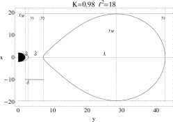
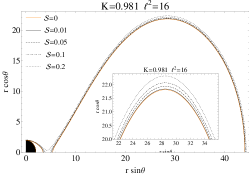
Figure 1: (Colour on-line)Left Case $B^{\phi}=0$: the closed Boyer surface at ${\rm{K}}=0.981$ and $\ell^{2}=18$: $\lambda\equiv y_{3}-y_{2}$ is the surface maximum diameter, $\delta\equiv y_{2}-2$ is the distance from the source, $\hat{\delta}\equiv y_{2}-y_{1}$ is the distance from the inner surface, $\breve{\delta}\equiv y_{1}-2$ is the distance of the inner surface from the horizon, $h\equiv 2x_{M}$ is the maximum thickness of the torus (torus height). Right Case $B^{\phi}\neq 0$: torus surface at ${\rm{K}}=0.981$ and $\ell^{2}=16$, in the plane $(r\sin\theta,r\cos\theta)$ for different values of $\mathcal{S}$. Inset figures are enlarged view of the main plot.

Consider $R_{s}$, for $\mathcal{S}\ll 1$:

$$R_{s}\approx R_{s}\left|{}_{\mbox{\tiny{($\mathcal{S}$=0)}}}\right.+\frac{dR_{s}}{dS}\left|{}_{\mbox{\tiny{($\mathcal{S}$=0)}}}\right.\mathcal{S},$$ (17)

where $R_{s}(\mathcal{S}=0)$ is the squeezing in the PD case $(\mathcal{S}=0)$, one can see this term as the hydrodynamic contribution to the disk squeezing. Where the approximation $\mathcal{S}\ll 1$ holds we can study the linear dependence of $R_{s}$ from $\mathcal{S}$. The case of increasing (decreasing ) squeezing with $\mathcal{S}$ is defined by $\left(\frac{dR_{s}}{dS}\left|{}_{\mbox{\tiny{($\mathcal{S}$=0)}}}\right.\right)>0\quad(\frac{dR_{s}}{dS}\left|{}_{\mbox{\tiny{($\mathcal{S}$=0)}}}\right.<0)$. The Boyer surfaces for $\mathcal{S}=0$ and $\mathcal{S}\neq 0$ are shown in figs. 1.

Remark: The magnetic pressure is regarded as a perturbation of the hydrodynamic component, it is assumed that the Boyer theory remains valid and applicable in this approximation (discussions on similar assumptions can be found in [9, 5]): the torus shape is determined by the equipotential surfaces which now are regulated in eq. (12) by an effective potential deformed, respect to the PD case ($B=0$), by the magnetic field. The approximation $\mathcal{S}\approx 0$ follows from this assumption. This analysis should be seen as a first attempt to compare the magnetic contribution to the torus dynamics respect to the kinetic pressure in terms of the torus squeezing. However, we have performed several numerical analysis by setting a solution of the family of magnetic fields assigning a fixed value for the parameter $q$. The range of this parameter is clearly divided into two regions, say $0<q<1$ and $q>1$, with a subrange with extreme $q=2$. The case $q=2$ is indeed interesting because the magnetic field loops wrap around with toroidal topology along the torus surface.

For $q<1$ the trend is clear: closed surfaces are roughly those studied in the case $q\approx 0$, for $q>1$ we get closed surfaces in the limit $\mathcal{S}\approx 0$, which is in agreement with expansion around $\mathcal{S}=0$, that is, when the contribution of the magnetic pressure to the torus dynamics is properly regarded as a perturbation with respect to the hydrodynamics solution, this is realized when an appropriate condition $(\mathcal{S}\ll 1)$ on the field parameters is satisfied. First we introduced the parameter $\mathcal{S}\equiv{\mathcal{M}q\omega^{q-1}}/(q-1)$ in eq. (13), then we expand eq. (13) around $\mathcal{S}=0$, and collect the terms up to first order. It should be noted that this equation, is equivalent to the corresponding obtained by an expansion in $q=0$, once ignored the terms ${\rm{K}}\mathcal{S}q$, and changing $\mathcal{S}\rightarrow-\mathcal{S}$ (by convention we are taking $\mathcal{S}>0$). The system analysed in eq. (15) is thus equivalent to the case of a torus with $\mathcal{S}=\left|\frac{\mathcal{M}q\omega^{-1+q}}{-1+q}\right|\approx 0$ and $(q{\rm{K}}\mathcal{S})=O[\mathcal{S}]$ (i.e. higher order than the 1th degree).

4 Squeezing of the Polish doughnuts

In this section we consider the squeezing of the PD model $(B^{\phi}=0)$. The PD torus has been extensively studied in the literature with both analytical and numerical methods, we refer in particular to [6] with which we share much of the notation and conventions used in this work. Setting $\mathcal{S}=0$ in eq. (15) we find

$$x=\pm\sqrt{\left[\frac{2\left({\rm{{\rm{K}}}}^{2}\ell^{2}+y^{2}\right)}{{\rm{{\rm{K}}}}^{2}\left(\ell^{2}-y^{2}\right)+y^{2}}\right]^{2}-y^{2}},$$ (18)

with $2\sqrt{2}/3<{\rm{K}}<1$ and angular momentum $({\ell}_{k}^{-})^{2}<{\ell^{2}}<({\ell}_{k}^{+})^{2}$, where ${\ell^{2}}_{k}^{-}>27/2$, we refer to [6] for the exact expression of ${\ell}_{k}^{\pm}$ and details. fig. 1-right shows a section of the PD torus for ${\rm{K}}=0.981$ and $\ell^{2}=18$. We summarize the results concerning the squeezing function $R_{s}=h/\lambda$ in the following.

The squeezing function $R_{s}$ increases monotonically with ${\rm{K}}$ and, at fixed ${\rm{K}}$ decreases with $\ell^{2}$, figs. 2.

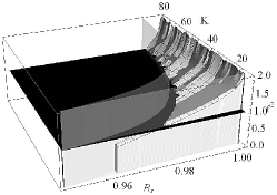
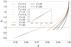
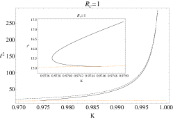
Figure 2: (Colour on-line) Case $B^{\phi}=0$. Left: The squeezing $R_{s}$ as function of ${\rm{K}}$ and the angular momentum $\ell^{2}$. The black plane is $R_{s}=1$, the curves $({\ell}_{k}^{\pm})^{2}$ are plotted. Center: $R_{s}$ curves for fixes values of the $\ell^{2}$ as function of ${\rm{K}}$, a zoom of the curves is in the inset plot: $R_{s}$ increases monotonically with ${\rm{K}}$ and, at fixed ${\rm{K}}$, decreases with $\ell^{2}$. Right: curve $R_{s}=1$ (black curve), orange dashed line is $(\ell_{k}^{-})^{2}$ black dashed line is $(\ell_{k}^{+})^{2}$, inside plot is a zoom of the $R_{s}=1$ in the region ${\rm{K}}\in[0.9735,0.975]$

This evolution can also be seen by studying of the function $\Delta_{s}\equiv h-\lambda$, shown in figs. 3,4 as function of $\ell$ and ${\rm{K}}$. However we note that the lower $R_{s}\equiv h/\lambda$ is and the thinner is the torus, conversely higher is $R_{s}$ and thicker is the torus. This therefore means that the toroidal surface is squeezed on the equatorial plane with decreasing ${\rm{K}}$ and increasing $\ell^{2}$. These results are indeed consistent with the analysis in [6] where it was shown that the torus thickness $h$, increases with the ${\rm{K}}$ and decreases with the angular momentum, that is the torus becomes thinner for high angular momenta, and thicker for high energies. The maximum diameter $\lambda$ increases with the ${\rm{K}}$, but decreases with the fluid angular momentum, moreover the location of maximum thickness of the torus moves towards the external regions with increasing angular momentum and ${\rm{K}}$, until it reaches a maximum an then decreases.

We note a region of $\ell$ and ${\rm{K}}$ values, in which this trend is reversed, that is $R_{s}=h/\lambda<1$ figs. 2- (left-center), and $\Delta_{s}=h-\lambda<0$ figs. 3,4-left, i.e. the squeezing is such that the disk is longer that thick, although the minimum value $R_{s}\approx 0.95$ is still quite large because it still makes sense that the model of PD be a thick disk. One sees from figs. 4, in this region, a minimum for $\Delta_{s}$ as a function of $\ell$. Following the curve for increasing values of ${\rm{K}}$, the function $\Delta_{s}$ decreases or decreases until it reaches a minimum and then increases. From fig. 2-center one also sees that the lower the angular momentum is and more configurations with $R_{s}<1$ are. Finally, some curves overlap in this region for one or more values of ${\rm{K}}$, this means that torus configurations would exist with different values of $\ell^{2}$, but equal ${\rm{K}}$ and $R_{s}$.

Fig. 2-right shows the solutions of equation $R_{s}=1$, on the curve $\ell^{2}({\rm{K}})$ . Essentially this curve confirms the previous results showing that the torus where the $(h)$ equals the length on the equatorial plane $\lambda$ increases in angular momentum with ${\rm{K}}$, first slowly and then more and more rapid as ${\rm{K}}$ approaches the value limit ${\rm{K}}=1$. A fixed $R_{s}$, the centrifugal effects must compensate for an increase of ${\rm{K}}$ which tends to bring the disk to a greater $R_{s}$, and to sufficiently small values of ${\rm{K}}\in(0.97367,0.9746)$, the curve bends back on itself, see Figs. 2.

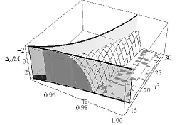
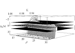
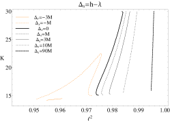
Figure 3: (Colour on-line) Case $B^{\phi}=0$. Left: difference $\Delta_{s}\equiv h-\lambda$ as function of ${\rm{K}}$ and $\ell^{2}$. Center plot shows $\Delta_{s}$ and the planes $\Delta_{s}=(0,\pm 2)$. Left: curves $\Delta_{s}=$cons as function of $\ell^{2}$ and ${\rm{K}}$.

5 Squeezing of the magnetized torus

In this section we summarize the analysis concerning the squeezing of the magnetized torus $(\mathcal{S}\neq 0)$.

Fig. 4 shows several surfaces $R_{s}(\ell^{2},{\rm{K}})$ for different values of $\mathcal{S}$, an enlarged view of this plot, distinguishes the different $\mathcal{S}$-surfaces. In general the function $R_{s}(\ell^{2},{\rm{K}})$, as for the case $\mathcal{S}=0$, increases with ${\rm{K}}$ but decreases with $\ell^{2}$ that is the torus is thicker as the ${\rm{K}}$ parameter increases and becomes thinner as fluid angular momentum increases, fig. 4-center, furthermore $R_{s}$ increases with $\mathcal{S}$, fig. 4,5-left.

The derivative $(dR_{s}/d\mathcal{S})(\mathcal{S}=0)$ is overwhelmingly positive: for the magnetized torus, $R_{s}$ grows with $\mathcal{S}$, hence the torus is thicker as $\mathcal{S}$ increases and thinner as $\mathcal{S}$ decreases, figs. 5,6-left. However, as evidenced by the Figs, 5,6 there is a small region $15.3\leq\ell^{2}\lesssim 16.65$, in which the derivative $(dR_{s}/d\mathcal{S})(\mathcal{S}=0)$ is negative and $R_{s}$ is a decreasing function of $\mathcal{S}$: from this we conclude that $R_{s}$ decreases compared to the case $\mathcal{S}=0$ i.e. the torus becomes thinner with increasing of $\mathcal{S}$ and viceversa becomes thicker to the decrease of $\mathcal{S}$, figs. 5.

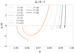
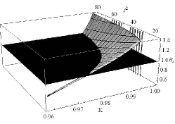
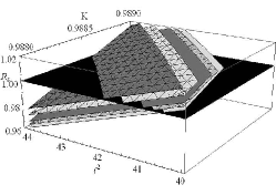
Figure 4: (Colour on-line) Left: Case $B^{\phi}=0$, plot of $\Delta_{s}$ as function of ${\rm{K}}$, for selected values of $\ell$. Case $B^{\phi}\neq 0$. Center: the squeezing $R_{s}$ as function of ${\rm{K}}$ and the angular momentum with $\ell^{2}$, for selected values of the $\mathcal{S}$ parameter. The black plane is $R_{s}=1$. A zoom is shown in right plot: white surface $\mathcal{S}=0$, shaded lightgray surface $\mathcal{S}=1/8$, gray surface $\mathcal{S}=1/4$, shaded white surface $\mathcal{S}=1/2$, shaded gray surface $\mathcal{S}=3/4$.

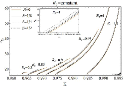
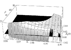
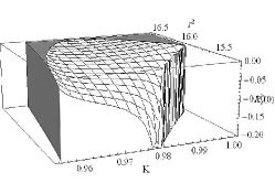
Figure 5: Case $B^{\phi}\neq 0$. Left: the squeezing surface $R_{s}=$cons for selected values of $\mathcal{S}$ as function of $\ell^{2}$ and ${\rm{K}}$. The inset plot shows the curves $R_{s}=1$ in the region ${\rm{K}}\in(.9765,.98)$ $\ell^{2}\in(20,24)$. Center: the function $R^{\prime}_{c}(0)\equiv dR_{s}/d\mathcal{S}$ in $\mathcal{S}=0$ as function of the $\ell^{2}$ and the parameter ${\rm{K}}$. The function is potted in the range $R^{\prime}_{c}(0)\in(-0.02,+0.02)$, black plane is $R^{\prime}_{c}(0)=0$. Right plot is a zoom in the region $R^{\prime}_{c}(0)\in(-0.02,0)0$, ${\rm{K}}\in(0.954,1)$, $\ell^{2}\in(15.3,16.65)$.

These results are confirmed in fig. 6, where the squeezing has been plotted as a function of $\mathcal{S}$ and $\ell^{2}$, for different values of ${\rm{K}}$, however it should be noted that although the figures show the behavior of the ratio $R_{s}$ across the range $0<\mathcal{S}<1$, the approximations assumed in this work are valuable for small $\mathcal{S}$. Fig. 6 shows that $R_{s}$ is generally increasing with ${\rm{K}}$ and decreasing with $\ell^{2}$, and also shows the existence of a region where this trend is reversed.

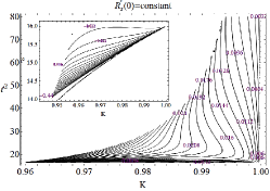
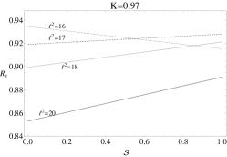
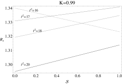
Figure 6: Case $B^{\phi}\neq 0$. Left: curves $R^{\prime}_{c}(0)=$constant in the plane $(\ell^{2},{\rm{K}})$, inside plot is a zoom in the region $\ell^{2}\in(15.3,16)$ where $R^{\prime}_{c}(0)<0$. Plot of the squeezing $R_{s}$ as function of $\mathcal{S}$ for selected values of $\ell^{2}$ and ${\rm{K}}=0.97$ (center plot), ${\rm{K}}=0.99$ (right plot). Plots show the range $\mathcal{S}\in[0,1]$, however the approximation $\mathcal{S}<<1$ holds for $\mathcal{S}<0.3$.

6 Conclusions

We have studied the Polish doughnut (PD) model of thick disk for a perfect fluid, circularly orbiting around a Black hole of Schwarzschild, in an hydrodynamic and magnetohydrodynamic context, using the effective potential approach examined in detail for the hydrodynamical model in [6]. For the magnetohydrodynamic model we used the solutions of the barotropic torus with a toroidal magnetic field discussed in [9, 10]. We have considered the magnetic contribution to the total pressure of the fluid as a perturbation of the effective potential for the exact full general relativistic part. Once defined the torus squeezing function $R_{s}\equiv h/\lambda$ as the ratio maximum torus height-to-maximum diameter of the torus section, we studied $R_{s}$ varying of the angular momentum $\ell$, the effective potential ${\rm{K}}$ and the parameter $\mathcal{S}$, the last evaluates the magnetic contribution to the fluid dynamics respect to the hydrodynamic contribution through its specific enthalpy. The lower is $R_{s}$ and the thinner is the torus, conversely the higher is $R_{s}$ and thicker is the torus. It is shown that given the presence of a magnetic pressure as a perturbation of the hydrodynamic component, there are not quantitatively significant effects on the thick disk model; however the analysis showed that the squeezing function has in general a monotonic trend with $(\ell,{\rm{K}},\mathcal{S})$. For the hydrodynamic case the squeezing function $R_{s}$ increases monotonically with ${\rm{K}}$, and at fixed ${\rm{K}}$ decreases with $\ell^{2}$, this therefore means that the toroidal surface is squeezed on the equatorial plane with decreasing “energy” ${\rm{K}}$ and increasing $\ell^{2}$, these results are indeed in agreement with analysis in [6]. However we observed a region of $\ell$ and ${\rm{K}}$ values, in which this trend is reversed, that is $R_{s}=h/\lambda<1$ reaching a minimum values of $R_{s}\approx 0.95$, for increasing values of ${\rm{K}}$, the squeezing decreases or decreases until it reaches a minimum and then increases. In the magnetohydrodynamic case, we evaluated the influence of the magnetic field through the parameter $\mathcal{S}$. In general, as for the case $\mathcal{S}=0$, the torus is thicker as the ${\rm{K}}$ parameter increases, and becomes thinner as fluid angular momentum increases, furthermore $R_{s}$ increases with $\mathcal{S}$. However there is a small region of $\ell$, in which $R_{s}$ is a decreasing function of $\mathcal{S}$: that is $R_{s}$ decreases compared to the case $\mathcal{S}=0$ i.e. the torus becomes thinner with increasing of $\mathcal{S}$ and viceversa becomes thicker with decreasing $\mathcal{S}$.

In conclusion, this analysis shows that the torus thickness is not modified in a quantitatively significant way by the presence of a toroidal magnetic field although it is much affected by the variation of the angular momentum. However we consider this analysis as a first attempt to compare the magnetic contribution to the torus dynamics with respect to the kinetic pressure in terms of the torus squeezing and, more in general, the plasma confinement in the disk toroidal surface.

- [1] Fender R., Belloni T., 2004, Ann. Rev. Astron. Astrophys., 42, 317.
- [2] Soria R., 2007, Astrophysics and Space Science, 311, 213.
- [3] Balbus S.A., 2011, Nat., 470, 475
- [4] Shakura N.I., Sunyaev R.A., 1973, A&A, 24, 337-355.
- [5] Abramowicz M. A. and Fragile P. C. , arXiv:1104.5499.
- [6] Pugliese D., Montani G. and Bernardini M. G., Mon. Not. Roy. Astron. Soc. , 428,(2012) 2, 952-982
- [7] R. H. Boyer, Proc. Cambridge Phil. Soc., 61:527, 1965.
- [8] Blaes O.M., 1987, MNRAS, 227, 975.
- [9] Komissarov S. S., MNRAS, 368 (2006) 993.
- [10] Montero P. J., Zanotti O., Font J. A. and Rezzolla L., MNRAS 378 (2007) 1101.
- [11] Horak J. and Bursa M., “Polarization from the oscillating magnetized accretion torus,” in R. Bellazzini, E. Costa, G. Matt and G. Tagliaferri X-ray Polarimetry, Cambridge University Press 2010, arXiv:0906.2420 .
- [12] Parker E. N., Astrophys. J. 122 (1955) 293.
- [13] Parker E. N., Astrophys. J. 160 (1970) 383.
- [14] Yoshizawa A., Itoh S. I, Itoh K., Plasma and Fluid Turbulence: Theory and Modelling, CRC Press, 2003.
- [15] Reyes-Ruiz M., Stepinski T. F., Astron. Astrophys. 342 (1999) 892 900.