Hamiltonian Dyson–Schwinger Equations of QCD

Abstract:

The general method for treating non-Gaussian wave functionals in the Hamiltonian formulation of a quantum field theory, which was previously developed and applied to Yang–Mills theory in Coulomb gauge, is generalized to full QCD. The Hamiltonian Dyson–Schwinger equations as well as the quark and gluon gap equations are derived and analysed in the IR and UV momentum regime. The back-reaction of the quarks on the gluon sector is investigated.

1 Introduction

Coulomb gauge Yang–Mills theory has attracted a considerable amount of attention over the last few years. In the continuum, both the Hamiltonian [1, 2, 3, 4] and the Lagrangian [5, 6, 7, 8] approach have been investigated. In the Hamiltonian approach, in particular, the use of variational methods with Gaussian wave functionals has led to the so-called gap equation for the inverse equal-time gluon propagator. The analytical and numerical solutions show an inverse gluon propagator which in the UV behaves like the photon energy but diverges in the IR, signalling confinement. The obtained propagator also compares favourably with the available lattice data [9]; deviations in the mid-momentum regime (and minor ones in the UV), which can be attributed to the gluon loop escaping the Gaussian wave functionals, can be taken into consideration by going beyond the purely Gaussian form. To treat these non-Gaussian functionals the authors developed in Ref. [10] a method relying on Dyson–Schwinger Equations (DSEs) by exploiting the formal similarity between vacuum expectation values in the Hamiltonian formalism and correlation functions in Euclidean quantum field theory. In this talk we report about the implementation of these techniques in the quark sector of the theory, in order to investigate issues like the spontaneous breaking of chiral symmetry.

The topic of chiral symmetry breaking in Coulomb gauge has been studied for example in Ref. [11]. While it has been shown that an infrared enhanced potential can account for chiral symmetry breaking, the calculated physical quantities, such as the dynamical mass and chiral condensate, turn out to be far too small. It has been recently shown [12] that using a wave functional which includes the coupling of the quarks to the transverse gluon field improves the results towards the phenomenological findings. We apply here the techniques developed in Ref. [10] to the wave functional proposed in Ref. [12]. While we do not expect considerably different results from Ref. [12] for physical quantities, the approach presented here has a broader range of applications, and could easily be applied to more complicated wave functionals.

2 Hamiltonian Dyson–Schwinger Equations

The derivation of the Hamiltonian DSEs in pure Yang–Mills theory has been presented in Ref. [10]. We summarize here briefly the essential steps leading from the choice of the wave functional to the pertinent DSEs.

In the Schrödinger picture of the Yang–Mills sector we represent the gauge field and the canonical momentum operators in the basis $|A\rangle$ of the eigenstates of the field operator by

$$\langle A\rvert\mkern 2.0mu\hat{A}\mkern 2.0mu\lvert\phi\rangle=A\,\varPhi[A],\qquad\langle A\rvert\mkern 2.0mu\hat{\Pi}\mkern 2.0mu\lvert\phi\rangle=\frac{\delta}{\mathrm{i}\,\delta A}\>\varPhi[A],$$ (1)

where $\varPhi[A]\equiv\langle A|\varPhi\rangle$ is a physical state. The vacuum expectation value (VEV) of an operator $K$ is therefore given by

$$\left<K[A,\Pi]\right>=\int\mathcal{D}A\>J_{A}\>\varPhi^{*}[A]\>K[A,\tfrac{\delta}{\mathrm{i}\delta A}]\>\varPhi[A].$$ (2)

In Eq. (2) the functional integration runs over transverse field configurations satisfying the Coulomb gauge condition, $\partial_{i}A_{i}^{a}=0$, and is restricted to the first Gribov region; $J_{A}=\operatorname{Det}(G_{A}^{-1})$ is the Faddeev–Popov determinant which arises from the gauge fixing, and

$$\bigl{[}G_{A}^{ab}({\vec{x}},{\vec{y}})\bigr{]}^{-1}=\bigl{(}-\delta^{ab}\partial^{2}-gf^{acb}A_{i}^{c}({\vec{x}})\partial_{i}\bigr{)}\delta({\vec{x}}-{\vec{y}})$$ (3)

is the inverse Faddeev–Popov operator, with $g$ being the coupling constant and $f^{abc}$ being the structure constants of the $\mathfrak{su}(N_{\mathrm{c}})$ algebra.

In a similar manner, a state $\lvert\varPhi\rangle$ in the fermionic Fock space possesses a “coordinate” representation

$$\langle\xi|\Phi\rangle\equiv\varPhi(\xi^{\dagger},\xi),$$ (4)

where $\xi$, $\xi^{\dagger}$ are complex Grassmann fields. The VEV of a fermionic operator in this state is given by

$$\left<\mathcal{O}[\hat{\psi},\hat{\psi}^{\dagger}]\right>=\int\mathcal{D}\xi^{\dagger}\,\mathcal{D}\xi\>\mathrm{e}^{-\xi^{\dagger}(\Lambda_{+}-\Lambda_{-})\xi}\>\varPhi^{*}(\xi,\xi^{\dagger})\>\mathcal{O}\bigl{[}\hat{\psi},\hat{\psi}^{\dagger}\bigr{]}\>\varPhi(\xi^{\dagger},\xi),$$ (5)

where the $\Lambda_{\pm}$ are the projectors onto states of positive and negative energy of the free Dirac theory. The Dirac field operators act on functionals according to

$$\begin{split}\hat{\psi}\varPhi(\xi^{\dagger},\xi)&=\left(\Lambda_{-}\xi+\Lambda_{+}\frac{\delta}{\delta\xi^{\dagger}}\right)\varPhi(\xi^{\dagger},\xi),\\ \hat{\psi}^{\dagger}\varPhi(\xi^{\dagger},\xi)&=\left(\Lambda_{+}\xi^{\dagger}+\Lambda_{-}\frac{\delta}{\delta\xi}\right)\varPhi(\xi^{\dagger},\xi).\end{split}$$ (6)

We have put explicitly a hat over the fermion operators $\hat{\psi}^{\dagger}$ in Eq. (6) to distinguish them from the Grassmann (classical) fields $\xi$, $\xi^{\dagger}$ used in the “coordinate” representation. The exponential factor occurring in the fermionic functional integration in Eq. (5) arises from the completeness relation for fermionic coherent states, see e.g. Ref. [13].

The vacuum state of QCD can be assumed to be of the form

$$\varPsi[A,\xi,\xi^{\dagger}]=\mathrel{\mathop{:}}\exp\left\{-\frac{1}{2}\,S_{A}[A]-S_{f}[\xi,\xi^{\dagger},A]\right\},$$ (7)

where $S_{A}$ is a functional of the gauge field only, while $S_{f}$ contains the fermion and fermion-gluon interaction parts. Dyson–Schwinger equations are derived by starting from the identity [10]

$$0=\int\mathcal{D}A\,\mathcal{D}\xi^{\dagger}\,\mathcal{D}\xi\>\frac{\delta}{\delta\phi}\left\{J_{A}\,\mathrm{e}^{-\xi^{\dagger}(\Lambda_{+}-\Lambda_{-})\xi}\>\varPsi^{*}[A,\xi,\xi^{\dagger}]\,K[A,\xi,\xi^{\dagger}]\,\varPsi[A,\xi,\xi^{\dagger}]\right\}$$ (8)

with $\phi\in\{A,\xi,\xi^{\dagger}\}$.

To proceed further, we need an explicit ansatz for the vacuum wave functional Eq. (7). Since we are interested here mainly in the quark sector, we choose the simple Gaussian form

$$S_{A}=\int\mathop{\mathrm{d}^{3}}\mkern-4.0mux\,\mathop{\mathrm{d}^{3}}\mkern-4.0muy\>A^{a}_{i}({\vec{x}})\,\omega({\vec{x}},{\vec{y}})\,A_{i}^{a}({\vec{y}})$$ (9)

for the Yang–Mills part. It should be stressed, however, that this is in no way necessary, and non-Gaussian generalization can be taken as well [10]; we restrict ourselves to the form Eq. (9) only for pedagogical reasons.

For the quark wave functional we choose the ansatz [12]

$$S_{f}=\int\mathop{\mathrm{d}^{3}}\mkern-4.0mux\,\mathop{\mathrm{d}^{3}}\mkern-4.0muy\>\xi_{+}^{m{\dagger}}({\vec{x}})\,K_{A}^{mn}({\vec{x}},{\vec{y}})\,\xi_{-}^{n}({\vec{y}}),\qquad\xi_{\pm}=\Lambda_{\pm}\xi.$$ (10)

The kernel $K_{A}$ contains both the purely fermionic part and the coupling of the quarks to the transverse gluons,

$$K_{A}^{mn}({\vec{x}},{\vec{y}})=\delta^{mn}\beta\,s({\vec{x}},{\vec{y}})+g\int\mathop{\mathrm{d}^{3}}\mkern-4.0muz\>V({\vec{x}},{\vec{y}};{\vec{z}})\,{\vec{\alpha}}\cdot{\vec{A}}^{a}({\vec{z}})\>t_{a}^{mn}.$$ (11)

Here, $\beta$ and ${\vec{\alpha}}$ are the usual Dirac matrices, $t_{a}$ are the generators of the group in the fundamental representation (or, in general, in the representation to which the fermion fields belong), and the functions $s$ and $V$ are the variational kernels.

With these choices for the wave functional the resulting DSEs are represented diagrammatically in Fig. 1.

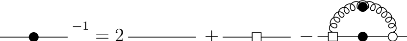
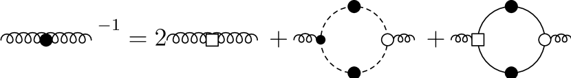
Figure 1: Hamiltonian DSEs for the quark (left) and gluon propagator (right). Filled dots stand for dressed propagators and empty circles for proper functions. The small empty boxes represent the variational kernels. Curly lines represent gluons, dashed lines ghosts, and straight lines fermions.

3 Variational Approach to QCD

The Hamilton operator of QCD in Coulomb gauge [14], resulting from the resolution of Gauss’s law in the canonically quantized theory, can be written as

$$H_{\mathrm{QCD}}=-\frac{1}{2}\int\mathop{\mathrm{d}^{3}}\mkern-4.0mux\>J_{A}^{-1}\frac{\delta}{\delta A_{i}^{a}({\vec{x}})}J_{A}\frac{\delta}{\delta A_{i}^{a}({\vec{x}})}+\frac{1}{4}\int\mathop{\mathrm{d}^{3}}\mkern-4.0mux\>F_{ij}^{a}({\vec{x}})\,F_{ij}^{a}({\vec{x}})\\ +\int\mathop{\mathrm{d}^{3}}\mkern-4.0mux\>\psi^{m{\dagger}}({\vec{x}})\bigl{[}-\mathrm{i}\alpha_{i}\partial_{i}+\beta\,m\bigr{]}\psi^{m}({\vec{x}})-g\int\mathop{\mathrm{d}^{3}}\mkern-4.0mux\>\psi^{m{\dagger}}({\vec{x}})\alpha_{i}A_{i}^{a}({\vec{x}})\,t_{a}^{mn}\psi^{n}({\vec{x}})\\ +\int\mathop{\mathrm{d}^{3}}\mkern-4.0mux\mathop{\mathrm{d}^{3}}\mkern-4.0muy\>J_{A}^{-1}\rho^{a}({\vec{x}})J_{A}\,F_{A}^{ab}({\vec{x}},{\vec{y}})\,\rho^{b}({\vec{y}}).$$ (12)

In Eq. (12)

$$F_{ij}^{a}({\vec{x}})=\partial_{i}A_{j}^{a}({\vec{x}})-\partial_{j}A_{i}^{a}({\vec{x}})+gf^{abc}A_{i}^{b}({\vec{x}})\,A_{j}^{c}({\vec{x}})$$ (13)

is the spatial part of the field strength tensor,

$$F_{A}^{ab}({\vec{x}},{\vec{y}})=\int\mathop{\mathrm{d}^{3}}\mkern-4.0muz\>G_{A}^{ac}({\vec{x}},{\vec{z}})\,(-\partial^{2}_{z})\,G_{A}^{cb}({\vec{z}},{\vec{y}})$$ (14)

is the so-called Coulomb kernel, which arises from the longitudinal component of the electric field, and

$$\rho^{a}({\vec{x}})=\psi^{m{\dagger}}({\vec{x}})t_{a}^{mn}\psi^{n}({\vec{x}})+f^{abc}A_{i}^{b}({\vec{x}})\frac{\delta}{\mathrm{i}\,\delta A_{i}^{c}({\vec{x}})}$$ (15)

is the total colour charge density.

The energy density can be evaluated as expectation value of the Hamiltonian Eq. (12). The Hamiltonian DSEs in the general form Eq. (8) enter this calculation twice: first to express the VEVs of the operators $\hat{\psi}$, $\hat{\psi}^{\dagger}$ in terms of the Grassmann fields $\xi$, $\xi^{\dagger}$, and second to turn the resulting expressions, which involve propagators and vertex functions, in a functional of the variational kernels. In this calculation we have to introduce approximations, and we evaluate the energy density up to two loops (see Ref. [10] for more details).

4 Gap Equations

The variation of the energy density with respect to $V$ fixes the vector kernel

$$V({\vec{p}},{\vec{q}})=-\frac{1+s({\vec{p}})\,s({\vec{q}})}{\Omega({\vec{p}}+{\vec{q}})+\lvert{\vec{p}}\rvert\frac{1-s^{2}({\vec{p}})+2s({\vec{p}})s({\vec{q}})}{1+s^{2}({\vec{p}})}+\lvert{\vec{q}}\rvert\frac{1-s^{2}({\vec{q}})+2s({\vec{p}})s({\vec{q}})}{1+s^{2}({\vec{q}})}},$$ (16)

where $\Omega=\tfrac{1}{2}\langle AA\rangle^{-1}$ is the inverse gluon propagator. Replacing the kernels occurring on the right-hand side by their tree-level forms, i.e. $\Omega({\vec{p}})=\lvert{\vec{p}}\rvert$ and $s({\vec{p}})=0$, we obtain

$$V_{0}({\vec{p}},{\vec{q}})=-\frac{1}{\lvert{\vec{p}}+{\vec{q}}\rvert+\lvert{\vec{p}}\rvert+\lvert{\vec{q}}\rvert},$$ (17)

which is exactly the leading-order perturbative expression for the quark-gluon vertex for massless fermions [15].

Equation (16) can be inserted back into the expression for the energy density, and taking functional derivatives with respect to $\omega({\vec{p}})$ and $s({\vec{p}})$ we obtain the gluon and quark gap equations. As a first approximation, we will ignore the $s$-dependence of the denominator of Eq. (16). Keeping the whole denominator structure would give rise to more complicated expressions which, however, have the same IR and UV asymptotic behaviour.

The approximated gap equation for the scalar quark kernel $s$ reads

$$\begin{split}\lvert{\vec{p}}\rvert\,s({\vec{p}})={}&\frac{g^{2}C_{F}}{2}\int{\frac{\mathrm{d}^{3}q}{(2\pi)^{3}}}\;F({\vec{p}}-{\vec{q}})\>\frac{s({\vec{q}})\bigl{[}1-s^{2}({\vec{p}})\bigr{]}-{\hat{p}}\cdot{\hat{q}}\,s({\vec{p}})\bigl{[}1-s^{2}({\vec{q}})\bigr{]}}{1+s^{2}({\vec{q}})}\\ &+\frac{g^{2}C_{F}}{2}\int{\frac{\mathrm{d}^{3}q}{(2\pi)^{3}}}\>\frac{X({\vec{p}},{\vec{q}})}{\Omega({\vec{p}}+{\vec{q}})}\frac{\bigl{[}1+s({\vec{p}})\,s({\vec{q}})\bigr{]}\bigl{[}s({\vec{q}})-s({\vec{p}})\bigr{]}}{\bigl{[}1+s^{2}({\vec{q}})\bigr{]}\,\bigl{[}\Omega({\vec{p}}+{\vec{q}})+\lvert{\vec{q}}\rvert+\lvert{\vec{p}}\rvert\bigr{]}},\end{split}$$ (18)

where $F=\langle F_{A}\rangle$ is the Coulomb propagator and $X$ is a tensor structure arising from the traces in Dirac space. The first term on the right-hand side of Eq. (18) was obtained by Adler and Davis [11]; the second term is due to the coupling of the quarks to the transverse gluons. As mentioned in the Introduction, in Ref. [12] the coupling to transverse gluons was also taken into account. The authors of Ref. [12] used the same wave functional Eq. (10) as in this work but did a quenched calculation. As a consequence the effect of the Yang–Mills kinetic energy operator on the quarks ws neglected.

Trading the scalar kernel $s$ in favour of the mass function $M$, Eq. (18) takes the following simple form

$$\begin{split}\lvert{\vec{p}}\rvert M({\vec{p}})={}&g^{2}\frac{C_{F}}{2}\int{\frac{\mathrm{d}^{3}q}{(2\pi)^{3}}}\;F({\vec{p}}-{\vec{q}})\frac{\lvert{\vec{p}}\rvert M({\vec{q}})-{\hat{p}}\cdot{\hat{q}}\,\lvert{\vec{q}}\rvert\,M({\vec{p}})}{\mathcal{E}({\vec{q}})}\\ &+g^{2}\frac{C_{F}}{2}\int{\frac{\mathrm{d}^{3}q}{(2\pi)^{3}}}\>\frac{X({\vec{p}},{\vec{q}})}{\Omega({\vec{p}}+{\vec{q}})\bigl{[}\Omega({\vec{p}}+{\vec{q}})+\lvert{\vec{p}}\rvert+\lvert{\vec{q}}\rvert\bigr{]}}\frac{\lvert{\vec{p}}\rvert M({\vec{q}})-\lvert{\vec{q}}\rvert M({\vec{p}})}{\mathcal{E}({\vec{q}})},\end{split}$$ (19)

with

$$\mathcal{E}({\vec{p}})=\sqrt{\smash[b]{{\vec{p}}^{2}+M^{2}({\vec{p}})}}.$$ (20)

The variation of the energy density with respect to the gluon kernel $\omega$ combined with the gluon propagator DSE yields the gap equation for inverse gluon propagator $\Omega$

$$\Omega^{2}({\vec{p}})={\vec{p}}^{2}+\text{Yang--Mills terms}\\ -g^{2}\int{\frac{\mathrm{d}^{3}q}{(2\pi)^{3}}}\frac{\bigl{[}1+s({\vec{q}})\,s({\vec{p}}+{\vec{q}})\bigr{]}^{2}}{\bigl{[}1+s^{2}({\vec{q}})\bigr{]}\bigl{[}1+s^{2}({\vec{p}}+{\vec{q}})\bigr{]}}\frac{2\Omega({\vec{p}})+\lvert{\vec{q}}\rvert+\lvert{\vec{p}}+{\vec{q}}\rvert}{\bigl{[}\Omega({\vec{p}})+\lvert{\vec{q}}\rvert+\lvert{\vec{p}}+{\vec{q}}\rvert\bigr{]}^{2}}\\ \times\left[1+\frac{{\vec{p}}\cdot{\vec{q}}+({\hat{p}}\cdot{\vec{q}})^{2}}{\lvert{\vec{q}}\rvert\,\lvert{\vec{p}}+{\vec{q}}\rvert}\right],$$ (21)

where the usual Yang–Mills terms (ghost loop, Coulomb interaction, and possibly additional terms stemming from a non-Gaussian ansatz) can be found in Ref. [10].

Equations (18) and (21) form a coupled system, toghether with the DSE for the ghost propagator and the Coulomb form factor. The analysis of the full coupled set of equations is subject of ongoing work. As a first estimate, we investigate the effect of the quark loop on the gluon propagator: we take the Gribov formula for the pure Yang–Mills gluon propagator and use for the scalar kernel $s$ a form fitted from the data in Ref. [12]. The result is plotted in Fig. 2.

Figure 2: Gluon propagator $D=1/(2\Omega)$ in the presence of quarks for the gap equation (21) assuming the Gribov form for the Yang–Mills part. Physical dimensions are set by the Coulomb string tension $\sigma_{\mathrm{C}}$.

As we see, the gluon propagator loses some stregth in the mid-momentum regime. This behaviour is known from Landau gauge studies, and Coulomb gauge investigations on the lattice confirm this [16].

5 Conclusions

The general method to treat non-Gaussian wave functionals in the Hamiltonian formulation of a quantum field theory presented in Ref. [10] has been applied here to QCD in Coulomb gauge. We have used the quark wave functional suggested in Ref. [12], which includes the coupling of the quarks to the transverse gluons. The resulting quark gap equations are similar in both approaches; the numerical solution of the equations and the comparison to the findings of Ref. [12] are the subject of ongoing work. As a first application we have presented here the effect of the back-coupling of the quarks on the gluon propagator. In future work we intend to expand the present approach to QCD at finite temperature [17] and baryon density.

References

- [1] D. Schutte, Phys. Rev. D31, 810–821 (1985).
- [2] A. P. Szczepaniak, and E. S. Swanson, Phys. Rev. D65, 025012 (2001).
- [3] C. Feuchter, and H. Reinhardt, Phys. Rev. D70, 105021 (2004).
- [4] D. Epple, H. Reinhardt, and W. Schleifenbaum, Phys. Rev. D75, 045011 (2007).
- [5] P. Watson, and H. Reinhardt, Phys. Rev. D75, 045021 (2007).
- [6] P. Watson, and H. Reinhardt, Phys. Rev. D77, 025030 (2008).
- [7] H. Reinhardt, and P. Watson, Phys. Rev. D79, 045013 (2009).
- [8] P. Watson, and H. Reinhardt, Phys. Rev. D82, 125010 (2010).
- [9] G. Burgio, M. Quandt, and H. Reinhardt, Phys. Rev. Lett. 102, 032002 (2009).
- [10] D. R. Campagnari, and H. Reinhardt, Phys. Rev. D82, 105021 (2010).
- [11] S. L. Adler, and A. Davis, Nucl. Phys. B244, 469 (1984).
- [12] M. Pak, and H. Reinhardt, Phys. Lett. B707, 566–569 (2012).
- [13] F. A. Berezin, The Method of Second Quantization, vol. 24 of Pure Appl. Phys., Academic Press, 1966.
- [14] N. H. Christ, and T. D. Lee, Phys. Rev. D22, 939–958 (1980).
- [15] D. R. Campagnari, Ph.D. thesis, Eberhard-Karls-Universität Tübingen (2010).
- [16] G. Burgio, private communication.
- [17] J. Heffner, H. Reinhardt, and D. R. Campagnari, Phys. Rev. D85, 125029 (2012).