Automated Variational Inference
in Probabilistic Programming

Abstract

We present a new algorithm for approximate inference in probabilistic programs, based on a stochastic gradient for variational programs. This method is efficient without restrictions on the probabilistic program; it is particularly practical for distributions which are not analytically tractable, including highly structured distributions that arise in probabilistic programs. We show how to automatically derive mean-field probabilistic programs and optimize them, and demonstrate that our perspective improves inference efficiency over other algorithms.

1 Introduction

1.1 Automated Variational Inference for Probabilistic Programming

Probabilistic programming languages simplify the development of probabilistic models by allowing programmers to specify a stochastic process using syntax that resembles modern programming languages. These languages allow programmers to freely mix deterministic and stochastic elements, resulting in tremendous modeling flexibility. The resulting programs define prior distributions: running the (unconditional) program forward many times results in a distribution over execution traces, with each trace generating a sample of data from the prior. The goal of inference in such programs is to reason about the posterior distribution over execution traces conditioned on a particular program output. Examples include BLOG [1], PRISM [2], Bayesian Logic Programs [3], Stochastic Logic Programs [4], Independent Choice Logic [5], IBAL [6], Probabilistic Scheme [7], $\Lambda_{\circ}$ [8], Church [9], Stochastic Matlab [10], and HANSEI [11].

It is easy to sample from the prior $p(x)$ defined by a probabilistic program: simply run the program. But inference in such languages is hard: given a known value of a subset $y$ of the variables, inference must essentially run the program ‘backwards’ to sample from $p(x|y)$. Probabilistic programming environments simplify inference by providing universal inference algorithms; these are usually sample based (MCMC or Gibbs) [9, 1, 6], due to their universality and ease of implementation.

Variational inference [12, 13, 14] offers a powerful, deterministic approximation to exact Bayesian inference in complex distributions. The goal is to approximate a complex distribution $p$ by a simpler parametric distribution $q_{\theta}$; inference therefore becomes the task of finding the $q_{\theta}$ closest to $p$, as measured by KL divergence. If $q_{\theta}$ is an easy distribution, this optimization can often be done tractably; for example, the mean-field approximation assumes that $q_{\theta}$ is a product of marginal distributions, which is easy to work with.

Since variational inference techniques offer a compelling alternative to sample based methods, it is of interest to automatically derive them, especially for complex models. Unfortunately, this is intractable for most programs. Even for models which have closed-form coordinate descent equations, the derivations are often complex and cannot be done by a computer. However, in this paper, we show that it is tractable to construct a stochastic, gradient-based variational inference algorithm automatically by leveraging compositionality.

2 Automated Variational Inference

An unconditional probabilistic program $f$ is defined as a parameterless function with an arbitrary mix of deterministic and stochastic elements. Stochastic elements can either belong to a fixed set of known, atomic random procedures called ERPs (for elementary random procedures), or be defined as function of other stochastic elements.

The syntax and evaluation of a valid program, as well as the definition of the library of ERPs, define the probabilistic programming language. As the program $f$ runs, it will encounter a sequence of ERPs $x_{1},\cdots,x_{T}$, and sample values for each. The set of sampled values is called the trace of the program. Let $x_{t}$ be the value taken by the $t^{\text{th}}$ ERP. The probability of a trace is given by the probability of each ERP taking the particular value observed in the trace:

$$p(x)=\prod_{t=1}^{T}p_{t}(x_{t}\>|\>\psi_{t}(h_{t}))$$ (1)

where $h_{t}$ is the history $(x_{1},\ldots,x_{t-1})$ of the program up to ERP $t$, $p_{t}$ is the probability distribution of the $t^{\text{th}}$ ERP, with history-dependent parameter $\psi_{t}(h_{t})$. Trace-based probabilistic programs therefore define directed graphical models, but in a more general way than many classes of models, since the language can allow complex programming concepts such as flow control, recursion, external libraries, data structures, etc.

2.1 KL Divergence

The goal of variational inference [13, 12, 14] is to approximate the complex distribution $p(x|y)$ with a simpler distribution $p_{\theta}(x)$. This is done by adjusting the parameters $\theta$ of $p_{\theta}(x)$ in order to maximize a reward function $L(\theta)$, typically given by the KL divergence:

$$KL(p_{\theta},p(x|y)) = \int_{x}p_{\theta}(x)\log\left(\frac{p_{\theta}(x)}{p(x|y)}\right)$$ (2)

$$= \int_{x}p_{\theta}(x)\log\left(\frac{p_{\theta}(x)}{p(y|x)p(x)}\right)+\log p(y)=-L(\theta)+\log p(y)$$

where (3)

$$L(\theta) \overset{\Delta}{=} \int_{x}p_{\theta}(x)\log\left(\frac{p(y|x)p(x)}{p_{\theta}(x)}\right)$$ (4)

Since the KL divergence is nonnegative, the reward function $L(\theta)$ is a lower bound on the partition function $\log p(y)=\log\int_{x}p(y|x)p(x)$; the approximation error is therefore minimized by maximizing the lower bound.

Different choices of $p_{\theta}(x)$ result in different kinds of approximations. The popular mean-field approximation decomposes $p_{\theta}(x)$ into a product of marginals as $p_{\theta}(x)=\prod_{t=1}^{T}p_{\theta}(x_{t}|\theta_{t})$, where every random choice ignores the history $h_{t}$ of the generative process.

2.2 Stochastic Gradient Optimization

Minimizing Eq. 2 is typically done by computing derivatives analytically, setting them equal to zero, solving for a coupled set of nonlinear equations, and deriving an iterative coordinate descent algorithm. However, this approach only works for conjugate distributions, and fails for highly structured distributions (such as those represented by, for example, probabilistic programs) that are not analytically tractable.

One generic approach to solving this is (stochastic) gradient descent on $L(\theta)$. We estimate the gradient according to the following computation:

$$-\nabla_{\theta}\>L(\theta) =\int_{x}\nabla_{\theta}\left(p_{\theta}(x)\log\left(\frac{p_{\theta}(x)}{p(y|x)p(x)}\right)\right)$$ (5)

$$=\int_{x}\nabla_{\theta}p_{\theta}(x)\left(\log\left(\frac{p_{\theta}(x)}{p(y|x)p(x)}\right)\right)+\int_{x}p_{\theta}(x)\left(\nabla_{\theta}\log(p_{\theta}(x))\right)$$ (6)

$$=\int_{x}\nabla_{\theta}p_{\theta}(x)\left(\log\left(\frac{p_{\theta}(x)}{p(y|x)p(x)}\right)\right)$$ (7)

$$=\int_{x}p_{\theta}(x)\nabla_{\theta}\log(p_{\theta}(x))\left(\log\left(\frac{p_{\theta}(x)}{p(y|x)p(x)}\right)\right)$$ (8)

$$=\int_{x}p_{\theta}(x)\nabla_{\theta}\log(p_{\theta}(x))\left(\log\left(\frac{p_{\theta}(x)}{p(y|x)p(x)}\right)+K\right)$$ (9)

$$\approx\frac{1}{N}\sum_{x^{j}}\nabla_{\theta}\log p_{\theta}(x^{j})\left(\log\left(\frac{p_{\theta}(x^{j})}{p(y|x^{j})p(x^{j})}\right)+K\right)$$ (10)

with $x^{j}\sim p_{\theta}(x)$, $j=1\ldots N$ and $K$ is an arbitrary constant. To obtain equations (7-9), we repeatedly use the fact that $\nabla\log p_{\theta}(x)=\frac{\nabla_{\theta}p_{\theta}(x)}{p_{\theta}(x)}$. Furthermore, for equations (7) and (9), we also use $\int_{x}p_{\theta}(x)\nabla\log p_{\theta}(x)=0$, since $\int_{x}p_{\theta}(x)\nabla\log p_{\theta}(x)=\int_{x}\nabla_{\theta}p_{\theta}(x)=\nabla_{\theta}\int_{x}p_{\theta}(x)=\nabla_{\theta}1=0$. The purpose of adding the constant $K$ is that it is possible to approximately estimate a value of $K$ (optimal baseline), such that the variance of the Monte-Carlo estimate (10) of expression (9) is minimized. As we will see, choosing an appropriate value of $K$ will have drastic effects on the quality of the gradient estimate.

2.3 Compositional Variational Inference

Consider a distribution $p(x)$ induced by an arbitrary, unconditional probabilistic program. Our goal is to estimate marginals of the conditional distribution $p(x|y)$, which we will call the target program. We introduce a variational distribution $p_{\theta}(x)$, which is defined through another probabilistic program, called the variational program. This distribution is unconditional, so sampling from it is as easy as running it.

We derive the variational program from the target program. An easy way to do this is to use a partial mean-field approximation: the target probabilistic program is run forward, and each time an ERP $x_{t}$ is encountered, a variational parameter is used in place of whatever parameters would ordinarily be passed to the ERP. That is, instead of sampling $x_{t}$ from $p_{t}(x_{t}\>|\>\psi_{t}(h_{t}))$ as in Eq. 1, we instead sample from $p_{t}(x_{t}\>|\>\theta_{t}(h_{t}))$, where $\theta_{t}(h_{t})$ is an auxiliary variational parameter (and the true parameter $\psi_{t}(h_{t})$ is ignored).

Fig. 1 illustrates this with pseudocode for a probabilistic program and its variational equivalent: upon encountering the normal ERP on line 4, instead of using parameter mu, the variational parameter $\theta_{3}$ is used instead (normal is a Gaussian ERP which takes an optional argument for the mean, and rand(a,b) is uniform over the set $[a,b]$, with $[0,1]$ as the default argument). Note that a dependency between $X$ and $M$ exists through the control logic, but not the parameterization. Thus, in general, stochastic dependencies due to the parameters of a variable depending on the outcome of another variable disappear, but dependencies due to control logic remain (hence the term partial mean-field approximation).

 Probabilistic program A  

1:   M = normal();

2:   if M$>$1

3:     mu = complex_deterministic_func( M );

4:     X = normal( mu );

5:   else

6:     X = rand();

7:   end;

 

 Mean-Field variational program A  

1:   M = normal( $\theta_{1}$ );

2:   if M$>$1

3:     mu = complex_deterministic_func( M );

4:     X = normal( $\theta_{3}$ );

5:   else

6:     X = rand($\theta_{4},\theta_{5}$);

7:   end;

 

Figure 1: A probabilistic program and corresponding variational program

This idea can be extended to automatically compute the stochastic gradient of the variational distribution: we run the forward target program normally, and whenever a call to an ERP $x_{t}$ is made, we:

• Sample $x_{t}$ according to $p_{\theta_{t}}(x_{t})$ (if this is the first time the ERP is encountered, initialize $\theta_{t}$ to an arbitrary value, for instance that given by $\psi_{t}(h_{t})$).

• Compute the log-likelihood $\log p_{\theta_{t}}(x_{t})$ of $x_{t}$ according to the mean-field distribution.

• Compute the log-likelihood $\log p(x_{t}|h_{t})$ of $x_{t}$ according to the target program.

• Compute the reward $R_{t}=\log p(x_{t}|h_{t})-\log p_{\theta}(x_{t})$

• Compute the local gradient $\psi_{t}=\nabla_{\theta_{t}}\log p_{\theta_{t}}(x_{t})$.

When the program terminates, we simply compute $\log p(y|x)$, then compute the gain $R=\sum R_{t}+\log p(y|x)+K$. The gradient estimate for the $t^{\text{th}}$ ERP is given by $R\psi_{t}$, and can be averaged over many sample traces $x$ for a more accurate estimate.

Thus, the only requirement on the probabilistic program is to be able to compute the log likelihood of an ERP value, as well as its gradient with respect to its parameters. Let us highlight that being able to compute the gradient of the log-likelihood with respect to natural parameters is the only additional requirement compared to an MCMC sampler.

Note that everything above holds: 1) regardless of conjugacy of distributions in the stochastic program; 2) regardless of the control logic of the stochastic program; and 3) regardless of the actual parametrization of $p(x_{t};\theta_{t})$. In particular, we again emphasize that we do not need the gradients of deterministic structures (for example, the function complex_deterministic_func in Fig. 1).

2.4 Extensions

Here, we discuss three extensions of our core ideas.

Learning inference transfer.  Assume we wish to run variational inference for $N$ distinct datasets $y^{1},\ldots,y^{N}$. Ideally, one should solve a distinct inference problem for each, yielding distinct $\theta^{1},\cdots,\theta^{N}$. Unfortunately, finding $\theta^{1},\cdots,\theta^{N}$ does not help to find $\theta^{N+1}$ for a new dataset $y_{N+1}$. But perhaps our approach can be used to learn ‘approximate samplers’: instead of $\theta$ depending on $y$ implicitly via the optimization algorithm, suppose instead that $\theta_{t}$ depends on $y$ through some fixed functional form. For instance, we can assume $\theta_{t}(y)=\sum_{j}\alpha_{i,j}f_{j}(y)$, where $f_{j}$ is a known function, then find parameters $\theta_{t,j}$ such that for most observations $y$, the variational distribution $p_{\theta(y)}(x)$ is a decent approximate sampler to $p(x|y)$. Gradient estimates of $\alpha$ can be derived similarly to Eq. 2 for arbitrary probabilistic programs.

Structured mean-field approximations.  It is sometimes the case that a vanilla mean-field distribution is a poor approximation of the posterior, in which case more structured approximations should be used [15, 16, 17, 18]. Deriving the variational update for structured mean-field is harder than vanilla mean-field; however, from a probabilistic program point of view, a structured mean-field approximation is simply a more complex (but still unconditional) variational program that could be derived via program analysis (or perhaps online via RL state-space estimation), with gradients computed as in the mean-field case.

Online probabilistic programming  One advantage of stochastic gradients in probabilistic programs is simple parallelizability. This can also be done in an online fashion, in a similar fashion to recent work for stochastic variational inference by Blei et al.  [19, 20, 21]. Suppose that the set of variables and observations can be separated into a main set $X$, and a large number $N$ of independent sets of latent variables $X_{i}$ and observations $Y_{i}$ (where the $(X_{i},Y_{i})$ are only allowed to depend on $X$). For instance, for LDA, $X$ represents the topic distributions, while the $X_{i}$ represent the document distribution over topics and $Y_{i}$ topic $i$. Recall the gradient for the variational parameters of $X$ is given by $K\psi_{X}$, with $K=R_{X}+\sum_{i}(R_{i}+\log P(Y_{i}|X_{i},X)$, where $R_{X}$ is the sum of rewards for all ERPs in $X$, and $R_{i}$ is the sum of rewards for all ERPs in $X_{i}$. $K$ can be rewritten as $X+NE[R_{v}+\log P(Y_{v}|X_{v},X)$, where $v$ is a random integer in $\{1,\ldots,N\}$. The expectation can be approximately computed in an online fashion, allowing the update of the estimate of $X$ without manipulating the entire data set $Y$.

3 Experiments: LDA and QMR

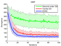
(a) Results on QMR

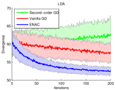
(b) Results on LDA

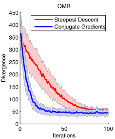
(c) Steepest descent vs. conjugate gradients

Figure 2: Numerical simulations of AVI

We tested automated variational inference on two common inference benchmarks: the QMR-DT network (a binary bipartite graphical model with noisy-or directed links) and LDA (a popular topic model). We compared three algorithms:

• The first is vanilla stochastic gradient descent on Eq. 2, with the gradients given by Eq. 5.

• The Episodic Natural Actor Critic algorithm, a version of the algorithm connecting variational inference to reinforcement learning – details are reserved for a longer version of this paper. An important feature of ENAC is optimizing over the baseline constant $K$.

• A second-order gradient descent (SOGD) algorithm which estimates the Fisher information matrix $F_{\theta}$ in the same way as the ENAC algorithm, and uses it as curvature information.

For each algorithm, we set $M=10$ (i.e., far fewer roll-outs than parameters). All three algorithms were given the same “budget” of samples; they used them in different ways. All three algorithms estimated a gradient $\hat{g}(\theta)$; these were used in a steepest descent optimizer: $\theta=\theta+\alpha\hat{g}(\theta)$ with stepsize $\alpha$. All three algorithms used the same stepsize; in addition, the gradients $g$ were scaled to have unit norm. The experiment thus directly compares the quality of the direction of the gradient estimate.

Fig. 2 shows the results. The ENAC algorithm shows faster convergence and lower variance than steepest descent, while SOGD fares poorly (and even diverges in the case of LDA). Fig. 2 also shows that the gradients from ENAC can be used either with steepest descent or a conjugate gradient optimizer; conjugate gradients converge faster.

Because both SOGD and ENAC estimate $F_{\theta}$ in the same way, we conclude that the performance advantage of ENAC is not due solely to its use of second-order information: the additional step of estimating the baseline improves performance significantly.

Once converged, the estimated variational program allows very fast approximate sampling from the posterior, at a fraction of the cost of a sample obtained using MCMC sampling. Samples from the variational program can also be used as warm starts for MCMC sampling.

4 Related Work

Natural conjugate gradients for variational inference are investigated in [25], but the analysis is mostly devoted to the case where the variational approximation is Gaussian, and the resulting gradient equation involves an integral which is not necessarily tractable.

The use of variational inference in probabilistic programming is explored in [29]. The authors similarly note that it is easy to sample from the variational program. However, they only use this observation to estimate the free energy of the variational program, but they do not estimate the gradient of that free energy. While they do highlight the need for optimizing the parameters of the variational program, they do not offer a general algorithm for doing so, instead suggesting rejection sampling or importance sampling.

Use of stochastic approximations for variational inference is also used by Carbonetto [30]. Their approach is very different from ours: they use Sequential Monte Carlo to refine gradient estimates, and require that the family of variational distributions contains the target distribution. While their approach is fairly general, it cannot be automatically generated for arbitrarily complex probabilistic models.

Finally, stochastic gradient methods are also used in online variational inference algorithms, in particular in the work of Blei et al. in stochastic variational inference (for instance, online LDA [19], online HDP [20], and more generally under conjugacy assumptions [21]), as a way to refine estimates of latent variable distributions without processing all the observations. However, this approach requires a manual derivation of the variational equation for coordinate descent, which is only possible under conjugacy assumptions which will in general not hold for arbitrary probabilistic programs.

References

- Milch et al. [2005] Brian Milch, Bhaskara Marthi, Stuart Russell, David Sontag, Daniel L. Ong, and Andrey Kolobov. BLOG: Probabilistic models with unknown objects. In International Joint Conference on Artificial Intelligence (IJCAI), pages 1352–1359, 2005.
- Sato and Kameya [1997] T. Sato and Y. Kameya. PRISM: A symbolic-statistical modeling language. In International Joint Conference on Artificial Intelligence (IJCAI), 1997.
- Kersting and Raedt [2007] K. Kersting and L. De Raedt. Bayesian logic programming: Theory and tool. In L. Getoor and B. Taskar, editors, An Introduction to Statistical Relational Learning. MIT Press, 2007.
- Muggleton [1996] Stephen Muggleton. Stochastic logic programs. In New Generation Computing. Academic Press, 1996.
- Poole [2008] David Poole. The independent choice logic and beyond. pages 222–243, 2008.
- Pfeffer [2001] Avi Pfeffer. IBAL: A probabilistic rational programming language. In International Joint Conference on Artificial Intelligence (IJCAI), pages 733–740. Morgan Kaufmann Publ., 2001.
- Radul [2007] Alexhey Radul. Report on the probabilistic language scheme. Technical Report MIT-CSAIL-TR-2007-059, Massachusetts Institute of Technology, 2007.
- Park et al. [2008] Sungwoo Park, Frank Pfenning, and Sebastian Thrun. A probabilistic language based on sampling functions. ACM Trans. Program. Lang. Syst., 31(1):1–46, 2008.
- Goodman et al. [2008] Noah Goodman, Vikash Mansinghka, Daniel Roy, Keith Bonawitz, and Joshua Tenenbaum. Church: a language for generative models. In Uncertainty in Artificial Intelligence (UAI), 2008.
- Wingate et al. [2011] David Wingate, Andreas Stuhlmueller, and Noah D. Goodman. Lightweight implementations of probabilistic programming languages via transformational compilation. In International Conference on Artificial Intelligence and Statistics (AISTATS), 2011.
- Kiselyov and Shan [2009] Oleg Kiselyov and Chung-chieh Shan. Embedded probabilistic programming. In Domain-Specific Languages, pages 360–384, 2009.
- Beal and MA [2003] M.J. Beal and M. MA. Variational algorithms for approximate bayesian inference. Unpublished doctoral dissertation, University College London, 2003.
- Jordan et al. [1999] Michael I. Jordan, Zoubin Ghahramani, and Tommi Jaakola. Introduction to variational methods for graphical models. Machine Learning, (37):183–233, 1999.
- Winn and Bishop [2006] J. Winn and C.M. Bishop. Variational message passing. Journal of Machine Learning Research, 6(1):661, 2006.
- Bouchard-Côté and Jordan [2009] A. Bouchard-Côté and M.I. Jordan. Optimization of structured mean field objectives. In Proceedings of the Twenty-Fifth Conference on Uncertainty in Artificial Intelligence, pages 67–74. AUAI Press, 2009.
- Ghahramani [1997] Z. Ghahramani. On structured variational approximations. University of Toronto Technical Report, CRG-TR-97-1, 1997.
- Bishop and Winn [2003] C.M. Bishop and J. Winn. Structured variational distributions in vibes. Proceedings Artificial Intelligence and Statistics, Key West, Florida, 2003.
- Geiger and Meek [2005] D. Geiger and C. Meek. Structured variational inference procedures and their realizations. In Proc. AIStats. Citeseer, 2005.
- Hoffman et al. [2010] M.D. Hoffman, D.M. Blei, and F. Bach. Online learning for latent dirichlet allocation. Advances in Neural Information Processing Systems, 23:856–864, 2010.
- [20] C. Wang, J. Paisley, and D.M. Blei. Online variational inference for the hierarchical dirichlet process.
- Blei [2011] D.M. Blei. Stochastic variational inference. 2011.
- Herbst [2010] Edward Herbst. Gradient and Hessian-based MCMC for DSGE models (job market paper), 2010.
- Wainwright and Jordan [2008] M.J. Wainwright and M.I. Jordan. Graphical models, exponential families, and variational inference. Foundations and Trends® in Machine Learning, 1(1-2):1–305, 2008.
- Peters et al. [2005] Jan Peters, Sethu Vijayakumar, and Stefan Schaal. Natural actor-critic. In European Conference on Machine Learning (ECML), pages 280–291, 2005.
- Honkela et al. [2008] A. Honkela, M. Tornio, T. Raiko, and J. Karhunen. Natural conjugate gradient in variational inference. In Neural Information Processing, pages 305–314. Springer, 2008.
- Amari [1998] S. Amari. Natural gradient works efficiently in learning. Neural Computation, (10), 1998.
- Kakade [2002] Sham A. Kakade. Natural policy gradient. In Neural Information Processing Systems (NIPS), 2002.
- Welling et al. [2008] M. Welling, Y.W. Teh, and B. Kappen. Hybrid variational/gibbs collapsed inference in topic models. In Proceedings of the Conference on Uncertainty in Artifical Intelligence (UAI), pages 587–594. Citeseer, 2008.
- Harik and Shazeer [2010] G. Harik and N. Shazeer. Variational program inference. Arxiv preprint arXiv:1006.0991, 2010.
- Carbonetto et al. [2009] P. Carbonetto, M. King, and F. Hamze. A stochastic approximation method for inference in probabilistic graphical models. In NIPS, volume 22, pages 216–224. Citeseer, 2009.