First results of an ${\rm H}\alpha$ based search of classical Be stars in the Perseus Arm and beyond

Abstract

We investigate a region of the Galactic plane, between $120^{\circ}\leq\ell\leq 140^{\circ}$ and $-1^{\circ}\leq b\leq+4^{\circ}$, and uncover a population of moderately reddened $(E(B-V)\sim 1)$ classical Be stars within and beyond the Perseus and Outer Arms. 370 candidate emission line stars $(13\lesssim r\lesssim 16)$ selected from the INT Photometric ${\rm H}\alpha$ Survey of the Northern Galactic plane (IPHAS) have been followed up spectroscopically. A subset of these, 67 stars with properties consistent with those of classical Be stars, have been observed at sufficient spectral resolution ($\Delta\lambda\approx 2$ – 4 Å) at blue wavelengths to narrow down their spectral types. We determine these to a precision estimated to be $\pm 1$ sub-type and then we measure reddenings via SED fitting with reference to appropriate model atmospheres. Corrections for contribution to colour excess from circumstellar discs are made using an established scaling to ${\rm H}\alpha$ emission equivalent width. Spectroscopic parallaxes are obtained after luminosity class has been constrained via estimates of distances to neighbouring A/F stars with similar reddenings. Overwhelmingly, the stars in the sample are confirmed as luminous classical Be stars at heliocentric distances ranging from 2 kpc up to $\sim$12  kpc. However, the errors are presently too large to enable the cumulative distribution function with respect to distance to distinguish between models placing the stars exclusively in spiral arms, or in a smooth exponentially-declining distribution.

1 Introduction

Outside the Solar Circle, the Perseus Arm is the first spiral arm crossed by Galactic Plane sight-lines. It contains a number of well-studied star-forming clouds (e.g. W3, W4 and W5, Megeath et al., 2008) set among stretches of relatively modest star-forming activity. The shape and characteristics of the Perseus Arm have been examined in several works over the years, using different tracers ranging from CO (Dame, Hartmann, & Thaddeus, 2001) through to OB associations (Russeil, 2003). A longstanding issue for these studies – particularly in the second quadrant of the Milky Way $(90^{\circ}\leq\ell\leq 180^{\circ})$ – has been the evidence for peculiar motions of stellar tracers and clouds, departing from the mean rotation law, which necessarily challenge kinematic distance determinations (e.g. Humphreys, 1976; Carpenter, Heyer, & Snell, 2000; Vallée, 2008). Recently, distances to star forming regions within the Perseus and other arms have begun to be measured reliably via methanol and OH maser trigonometric parallaxes, known to milli-arcsec precision. Of special significance to the present study is the Xu et al. (2006) result for W3OH ($\ell\simeq 134^{\circ}$) in the Perseus Arm, from which a distance of 1.95 $\pm$ 0.04 kpc was obtained. This represented a shortening of scale that has now been absorbed within the new consensus as may be found in the works of Russeil, Adami, & Georgelin (2007) and Vallée (2008).

Beyond the Perseus Arm, also within the second quadrant, there is some evidence accumulating in favour of the existence of a further spiral arm, which is referred to as either the Outer or Cygnus Arm. Russeil (2003), Russeil, Adami, & Georgelin (2007), Levine, Blitz, & Heiles (2006) and Steiman-Cameron, Wolfire, & Hollenbach (2010) have identified stellar and gaseous tracers, that lend support to this outer structure. Nevertheless, its location and true character remains elusive because of present limits on the quantity of tracers available combined with the continuing need to make significant use of kinematic distances. For the Outer Arm, a distance between 5 – 6 kpc, is quoted from fits of logarithmic spirals to the relevant tracers (Russeil, 2003; Vallée, 2008). Negueruela & Marco (2003) also estimated a distance range running from 5 to 6 kpc, via photometric parallaxes of a sample of bright OB stars. The best single measurement to date is the maser parallax obtained for WB89-437 by Hachisuka et al. (2009), giving a distance of 6.0$\pm$0.2 kpc. At these distances, the Outer Arm straddles the zone of Galacto-centric radii ($13\lesssim R_{G}\lesssim 14$ kpc) in which the stellar disc ’truncates’ (Ruphy et al., 1996) or, as has now become clear, presents a pronounced shortening of exponential length scale (Sale et al., 2010).

So whilst the reality of at least the Perseus Arm is beyond doubt, a settled picture of the Galactic Plane in the second quadrant is yet to emerge. In this paper, we add to the pool of available tracers a first sample of reddened classical Be (CBe) stars, reaching down to $r\approx 16$, that is drawn from the INT/WFC Photometric H$\alpha$ Survey of the Northern Galactic Plane (IPHAS) (Drew et al., 2005) and in particular the catalogue of ${\rm H}\alpha$ emission line sources provided in Witham et al. (2008). In so doing we point towards the gain to be had from more comprehensive exploitation of these newly available emission line objects.

CBe stars are mainly early B-type stars of luminosity class V-III that are on the Main-Sequence (MS) or moving off it (Porter & Rivinius, 2003). They are frequently observed in young open clusters ($\leq 30$ Myr) (Fabregat & Torrejón, 2000), and their spectra exhibit allowed transitions in emission (mainly lower excitation Balmer lines). Earlier CBe stars at least have not had time to move far from their birth places but, equally, they are unlikely to be heavily embedded in their parental clouds. In addition they are intrinsically bright, with absolute magnitudes ranging from $\sim 0$ down to $\sim-4$, enabling their detection at great distances across the Galactic Plane. In combination, these attributes make them highly suitable targets for studying spiral arm structure.

We focus our study in a patch of sky, spanning $100\,\rm{deg}^{2}$, that covers the Perseus Arm in the Galactic longitude range $120\degr\leq\ell\leq 140\degr$ and latitude band $-1\degr\leq b\leq+4\degr$. The positive offset of the chosen latitude band ensures we capture the displacement of the Galactic mid-plane caused by warping – a phenomenon that is evident both from maps of H I and dust emission (Freudenreich et al., 1994) and from the distribution of star forming complexes (Russeil, 2003). The selected longitude range encompasses the much-studied star forming complex W3/W4/W5, along with a more quiescent stretch of the Perseus Arm.

We present the results of a two-stage spectroscopic follow-up programme. The process begins with low resolution spectroscopy of $\sim$370 photometrically-selected candidate emission line objects – the brighter portion of a total population in this part of the Plane, of more than 560 candidate emission line stars (Section 2). This sample is further reduced to a set of 67 stars, for which we have medium-resolution spectra that ultimately serve to confirm the selected objects are nearly all luminous CBe stars. In Section 3, we determine spectral types and colour excesses for this sample and then estimate the contribution to the colour excess that originates in the circumstellar disc (that adds on to the interstellar component), which is observed toward each star. Using IPHAS survey data, we compare the resultant spectroscopic parallaxes with distances to similarly-reddened non-emission line A/F stars within a few arcminutes of each CBe star, in order to set constraints on luminosity class. This is described in Section 4, where we also present the spatial distribution of CBe stars that we obtain. Some of the sample appear to be very distant ($R_{G}\geq 13$ kpc) early-type CBe stars. The paper ends with a discussion that includes consideration of how the derived spatial distribution compares with simple simulations, accounting for typical errors, that place the stars either within the spiral arms only, or distributes them smoothly according to an exponential stellar density profile. We also consider how the derived CBe star colour excesses compare with total integrated values from the map of Schlegel, Finkbeiner, & Davis (1998, hereafter, SFD98).

2 Spectroscopic follow-up of bright candidate emission line stars

2.1 Low resolution spectroscopy

Candidate emission line stars in the specified Perseus Arm region (Galactic longitude range $120\degr\leq\ell\leq 140\degr$, latitude range $-1\degr\leq b\leq+4\degr$) were identified from the Witham et al. (2008) catalogue as potential spectroscopy targets. All such objects are point sources that exhibit a clear $(r-{\rm H}\alpha)$ excess, with respect to main-sequence stars in the $(r-H\alpha,\,r-i)$ colour-colour diagram: 560 such candidates fall within the chosen sky area, in the magnitude range $13\leq r\leq 19.5$. To enable spectroscopic follow-up on small to mid-sized telescopes, we restricted this sample to objects brighter than $r\approx 16$, i.e. 354 of them. To this list, we then added a further $\sim 50$ emission-line candidates ($13\lesssim r\lesssim 16$) derived from IPHAS photometry that was not available at the time the Witham et al. (2008) catalogue was compiled.

Observations of most of this moderately bright sample were collected between 2005 and 2011 at the 1.5m Fred Laurence Whipple Observatory (FLWO) Tillinghast Telescope using the FAST spectrograph (Fabricant et al., 1998). All in all, 370 objects were observed. The resolution of the spectra obtained was $\Delta\lambda\simeq 6$ Å, and the data span the wavelength range 3500 – 7500 Å. The spectra from this facility were obtained in queue mode, and pipeline-processed at the Telescope Data Center at the Smithsonian Astrophysical Observatory. They were delivered without relative flux calibration. An approximate calibration was applied to them subsequently, using a number of spectrophotometric standards taken from the FLWO-1.5m/FAST archive.

Fig. 1 shows the IPHAS colours of the observed target stars that were confirmed by visual inspection of their spectra to be genuine ${\rm H}\alpha$ emitters ($>90$% of the 370 observed targets). The photometric colours are derived using an internal release of the forthcoming global calibration of IPHAS (Farnhill et al. in prep). Fig. 2 shows the spatial distribution of the observed sample of targets. In both figures we pick out, in advance of discussion, the colours and positions of the 67 CBe stars for which we have acquired mid-resolution spectra.

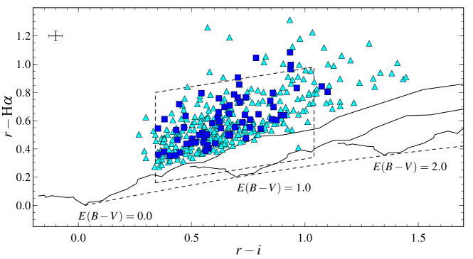
Figure 1: IPHAS colour-colour diagram of the observed targets (cyan triangles). Black solid lines are synthetic main sequence loci, at $E(B-V)$ = 0.0, 1.0, 2.0 (see e.g. Table 2 in Drew et al., 2005). These move parallel to the reddening vector that is plotted as the early-A reddening curve (dashed lower curve). The box drawn above the unreddened main sequence defines the region in which CBe stars with $A_{v}\sim 4$ are likely to be located (cf Fig. 3 and the discussion to be found in Corradi et al. (2008).The CBe stars, for which we have obtained intermediate-resolution spectra, are picked out as blue squares. Typical error bars are plotted in the upper left corner.

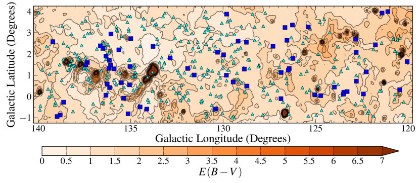
Figure 2: A contour map of integrated dust column across the area, from SFD98: the highest reddening contour drawn is for $E(B-V)=7$. The spatial distribution of the candidate emission line stars is superposed. Symbols and colour scheme are the same as in Fig. 1.

2.2 Further reduction of the sample

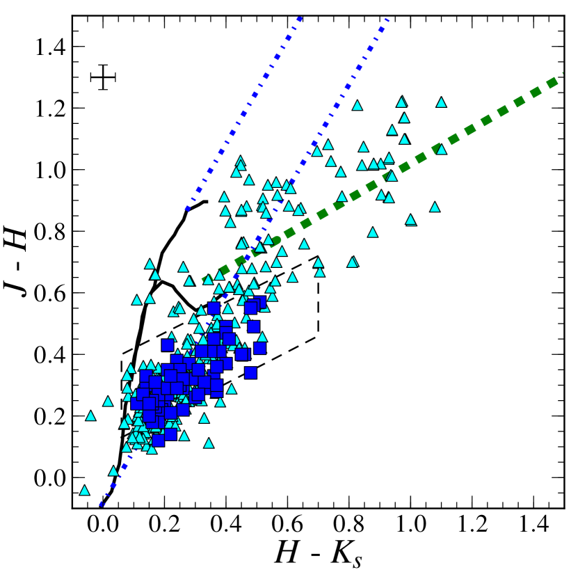
Figure 3: 2MASS near-infrared colour-colour diagram of our sample. The colour symbols are as in Fig. 1. The solid line follows the dwarf and giant unreddened sequences (Bessell & Brett, 1988). The blue dot-dashed lines are the reddening vectors from Rieke & Lebofsky (1985). The box drawn is due to Corradi et al. (2008) and roughly delineates the region CBe stars with $A_{V}\sim 4$ would occupy, while the green dashed line is the CTTS locus (Meyer, Calvet, & Hillenbrand, 1997). All the plotted curves are converted to the 2MASS system, adopting relationships defined in Carpenter (2001). Typical error bars are in the upper left corner of the diagram.

The FLWO-1.5m/FAST observations have allowed us to cover a large part of the potential target list for this region of sky, in order to confirm/reject the emission line star status of the candidates, confirming a high success rate for IPHAS candidate emitter selection. The combination of achieved signal-to-noise ratio (S/N) and spectral resolution is sufficient for a first-pass coarse typing, allowing early-type emission line stars to be clearly distinguished from late-type.

The identification of suitable targets for further evaluation via intermediate resolution spectroscopy, relied on two features that are frequently shared with other classes of emission line star and so must be appraised carefully:

1. The bright ${\rm H}\alpha$ emission, originating in the circumstellar environment of classical Be stars (Porter & Rivinius, 2003), which is now known to originate from a disc (Dachs, Rohe, & Loose, 1990, and references therein). Similarly strong $H\alpha$ emission is also observed both in low-mass YSOs, or classical T-Tauri stars (CTTS) (Bertout, 1989), and in intermediate-mass ones, or Herbig Ae/Be stars (HAeBe) (Waters & Waelkens, 1998). Very nearly all the confirmed emission line stars are either CBe stars or YSOs. A property that can provide some discrimination is the presence/absence of nebular forbidden line emission. CBe-star spectra do not in general present with forbidden line emission. Any objects presenting such features are not included in the sample discussed here.

2. A critical diagnostic separating CBe from candidate YSOs is accessed at near-infrared (NIR) wavelengths. The spectral energy distributions (SED) of optically-visible YSOs present a NIR colour excess due to thermal emission from a circumstellar disc. The scale of the excess depends on their evolutionary stage and type of object (see e.g. Lada & Adams, 1992; Meyer, Calvet, & Hillenbrand, 1997). But here the important point is that, by comparison with that of YSOs, the NIR excess characteristic of CBe stars (due to circumstellar free-free emission) is very much weaker.

We therefore supplemented IPHAS photometry and our low-resolution spectroscopy with 2MASS photometry (Cutri et al., 2003) in order to help distinguish likely CBe stars from YSOs (and other emission line stars). We required definite detections in all three 2MASS bands (quality flags A, B or C) as minimum (i.e. 367 objects). Then the measured $(J-H)$, $(H-K)$ colours must place the object in the domain close to or redward of the line traced by non-emission early type stars as they redden. There is some expectation that as $(H-K)$ grows, YSOs or similar objects with strong NIR excesses may begin to mix in with the CBe stars. Our final sample of 67 CBe stars is drawn from those with NIR colours bluer than $(J-H)=0.6$. This removes from consideration altogether, objects that may be red enough in $(J-H)$ to be lightly-reddened CTTSs.

Fig. 3 shows the 2MASS colour-colour diagram of all potential targets: triangles distinguish objects with only low-resolution spectra and squares those deemed to be probable CBe stars that were selected for further spectroscopy at intermediate spectral resolution. The number of objects that could have satisfied all our selection criteria is 230 (out of 367). The IPHAS and 2MASS photometry for the sample of 67 objects scrutinised here is collected into Table 1.

Our final selection exhibits the same broad range of reddenings, $2\lesssim A_{V}\lesssim 5$ present in the total available sample: accordingly these objects’ NIR colours are shifted parallel to the blue dot-dashed lines drawn in Fig. 3 that are themselves parallel to the reddening vector. To underline this point we have drawn in Fig. 3, the $A_{V}\sim 4$ Be-star selection region presented in the analysis of Corradi et al. (2008) and note that most of the target stars fall within it. That the reddening is significant is consistent with the presence of well-developed diffuse interstellar bands (DIB) in the spectra of the majority of our selected targets.

Next, in Section 2.3, we describe our intermediate-resolution spectroscopy of this reduced sample and the reduction techniques that we adopted.

Table 1: IPHAS and 2MASS photometry of the 67 CBe stars, with intermediate-resolution spectra. Objects will be identified by their (#) number, as given in this table in the rest of the paper. Columns are: IPHAS point-source name, which includes the J2000 RA and Dec; Galactic coordinates; $r$ magnitude, $(r-i)$ and $(r-{\rm H}\alpha)$ colours from IPHAS; $J$ magnitudes, $(J-H)$ and $(H-K)$ colours from 2MASS. The errors on the $r$ magnitudes and the ($r-i$, $r-{\rm H}\alpha$) colours are dominated by the photometric calibration and are respectively $0.02$, $0.03$, $0.035$.

#	IPHAS	$\ell$	b	$r$	$(r-i)$	$(r-{\rm H}\alpha)$	$J$	$(J-H)$	$(H-K)$
	Jhhmmss.ss+ddmmss.s	(deg)	(deg)	(mag)	(mag)	(mag)	(mag)	(mag)	(mag)
1	J002441.73+642137.5	120.04	1.64	14.76	0.86	0.61	$12.51\pm 0.02$	$0.30\pm 0.04$	$0.26\pm 0.04$
2	J002926.93+630450.2	120.45	0.32	14.07	0.35	0.36	$13.11\pm 0.02$	$0.12\pm 0.04$	$0.17\pm 0.04$
3	J003248.02+664759.6	121.09	3.99	14.46	0.96	0.83	$12.11\pm 0.02$	$0.55\pm 0.03$	$0.36\pm 0.03$
4	J003559.30+664502.9	121.40	3.92	15.96	0.76	0.61	$14.11\pm 0.04$	$0.40\pm 0.06$	$0.47\pm 0.06$
5	J004014.89+651644.0	121.76	2.43	14.79	0.70	0.76	$12.95\pm 0.02$	$0.29\pm 0.04$	$0.26\pm 0.05$
6	J004517.08+640124.1	122.26	1.16	15.62	0.89	0.64	$13.37\pm 0.02$	$0.41\pm 0.04$	$0.38\pm 0.04$
7	J004651.69+625914.3	122.41	0.12	14.87	0.50	0.45	$13.32\pm 0.02$	$0.22\pm 0.04$	$0.26\pm 0.05$
8	J005011.89+633525.8	122.79	0.72	15.37	0.62	0.62	$13.69\pm 0.02$	$0.28\pm 0.04$	$0.37\pm 0.05$
9	J005012.69+645621.6	122.80	2.07	14.16	0.55	0.48	$12.65\pm 0.03$	$0.30\pm 0.05$	$0.14\pm 0.05$
10	J005029.25+653330.8	122.83	2.69	14.65	0.67	0.65	$12.97\pm 0.03$	$0.26\pm 0.04$	$0.30\pm 0.04$
11	J005436.84+630549.9	123.29	0.23	14.95	0.62	0.76	$13.30\pm 0.03$	$0.33\pm 0.05$	$0.36\pm 0.05$
12	J005611.62+630350.5	123.47	0.20	14.37	0.50	0.47	$12.95\pm 0.02$	$0.18\pm 0.03$	$0.18\pm 0.03$
13	J005619.50+625824.0	123.49	0.11	14.61	0.38	0.38	$13.46\pm 0.02$	$0.23\pm 0.03$	$0.20\pm 0.04$
14	J010045.58+631740.2	123.98	0.44	15.41	0.73	0.64	$13.53\pm 0.02$	$0.32\pm 0.04$	$0.29\pm 0.05$
15	J010707.68+625117.0	124.72	0.04	14.56	0.72	0.59	$12.65\pm 0.02$	$0.39\pm 0.03$	$0.24\pm 0.03$
16	J010958.80+625229.3	125.04	0.08	14.09	0.86	0.70	$12.44\pm 0.02$	$0.47\pm 0.04$	$0.40\pm 0.04$
17	J011543.94+660116.1	125.40	3.27	14.14	0.93	1.08	$11.95\pm 0.02$	$0.49\pm 0.04$	$0.40\pm 0.04$
18	J012158.74+642812.8	126.22	1.79	14.31	0.71	0.73	$12.74\pm 0.03$	$0.29\pm 0.05$	$0.33\pm 0.05$
19	J012405.42+660059.9	126.25	3.36	14.98	0.63	0.55	$13.45\pm 0.03$	$0.27\pm 0.04$	$0.21\pm 0.04$
20	J012320.10+635830.7	126.42	1.32	14.02	0.94	0.97	$11.89\pm 0.02$	$0.47\pm 0.03$	$0.40\pm 0.03$
21	J012339.76+635312.9	126.47	1.24	15.00	0.85	0.74	$12.96\pm 0.02$	$0.41\pm 0.03$	$0.35\pm 0.03$
22	J012609.27+651617.7	126.55	2.64	14.72	0.91	0.64	$12.79\pm 0.03$	$0.45\pm 0.04$	$0.35\pm 0.04$
23	J012751.29+655104.0	126.65	3.24	14.49	0.74	0.76	$12.77\pm 0.02$	$0.37\pm 0.04$	$0.28\pm 0.04$
24	J012703.24+634333.2	126.86	1.13	14.00	0.86	0.80	$11.60\pm 0.02$	$0.37\pm 0.04$	$0.40\pm 0.04$
25	J012540.54+623025.6	126.87	-0.10	13.34	0.55	0.51	$12.05\pm 0.02$	$0.22\pm 0.03$	$0.19\pm 0.02$
26	J013245.66+645233.2	127.30	2.36	15.36	0.78	1.04	$13.31\pm 0.03$	$0.47\pm 0.04$	$0.40\pm 0.05$
27	J014218.74+624733.5	128.71	0.49	14.53	0.67	0.49	$12.90\pm 0.03$	$0.30\pm 0.04$	$0.23\pm 0.04$
28	J014620.44+644802.5	128.74	2.55	14.37	0.48	0.44	$13.25\pm 0.03$	$0.23\pm 0.04$	$0.17\pm 0.04$
29	J014458.14+633244.0	128.85	1.29	13.97	0.50	0.44	$12.89\pm 0.02$	$0.17\pm 0.04$	$0.16\pm 0.04$
30	J015037.67+644446.9	129.19	2.60	14.59	0.45	0.37	$13.52\pm 0.03$	$0.21\pm 0.04$	$0.23\pm 0.04$
31	J014905.18+624912.3	129.46	0.68	13.71	0.87	0.61	$11.49\pm 0.02$	$0.34\pm 0.04$	$0.48\pm 0.04$
32	J015918.32+654955.8	129.81	3.87	15.14	0.53	0.50	$13.80\pm 0.02$	$0.24\pm 0.03$	$0.16\pm 0.04$
33	J015246.27+630315.0	129.82	1.00	14.35	0.57	0.40	$12.90\pm 0.02$	$0.25\pm 0.04$	$0.18\pm 0.04$
34	J015613.22+635623.8	129.97	1.96	14.05	0.47	0.63	$12.82\pm 0.03$	$0.31\pm 0.04$	$0.33\pm 0.04$
35	J015922.53+635829.3	130.30	2.08	15.06	0.54	0.79	$13.37\pm 0.02$	$0.45\pm 0.03$	$0.36\pm 0.03$
36	J015427.15+612204.7	130.41	-0.59	14.29	1.07	0.84	$11.55\pm 0.02$	$0.57\pm 0.03$	$0.51\pm 0.02$
37	J020734.24+623601.1	131.56	1.01	14.42	0.60	0.44	$12.98\pm 0.02$	$0.27\pm 0.04$	$0.18\pm 0.04$
38	J021121.67+624707.5	131.92	1.32	15.54	0.67	0.50	$13.93\pm 0.03$	$0.35\pm 0.05$	$0.25\pm 0.05$
39	J022033.45+625717.4	132.86	1.81	15.75	0.71	0.86	$13.90\pm 0.02$	$0.40\pm 0.04$	$0.45\pm 0.04$
40	J022953.82+630742.3	133.79	2.35	14.31	0.66	0.50	$12.85\pm 0.02$	$0.22\pm 0.03$	$0.15\pm 0.03$
41	J022337.05+601602.8	134.13	-0.59	14.00	0.57	0.50	$12.54\pm 0.02$	$0.25\pm 0.02$	$0.16\pm 0.03$
42	J022635.99+601401.8	134.49	-0.49	14.54	0.94	0.99	$12.13\pm 0.02$	$0.56\pm 0.02$	$0.49\pm 0.03$
43	J024054.96+630009.7	134.99	2.72	15.72	0.43	0.53	$14.36\pm 0.03$	$0.29\pm 0.05$	$0.21\pm 0.07$
44	J023642.66+614714.9	135.03	1.41	15.44	0.56	0.39	$13.95\pm 0.05$	$0.33\pm 0.07$	$0.14\pm 0.06$
45	J023404.70+605914.4	135.06	0.55	12.91	0.62	0.66	$11.30\pm 0.02$	$0.42\pm 0.03$	$0.52\pm 0.03$
46	J023031.39+594127.1	135.14	-0.81	14.49	0.57	0.43	$12.96\pm 0.02$	$0.31\pm 0.04$	$0.17\pm 0.04$
47	J023431.07+601616.6	135.38	-0.08	13.62	1.10	0.80	$10.77\pm 0.02$	$0.55\pm 0.03$	$0.48\pm 0.04$
48	J023744.52+605352.8	135.50	0.65	16.79	0.74	0.48	$14.76\pm 0.04$	$0.28\pm 0.07$	$0.31\pm 0.09$
49	J024405.38+621448.7	135.64	2.19	15.24	0.44	0.46	$13.80\pm 0.02$	$0.49\pm 0.03$	$0.49\pm 0.04$
50	J024252.57+611953.9	135.89	1.30	15.75	0.70	0.91	$13.95\pm 0.03$	$0.36\pm 0.05$	$0.37\pm 0.05$
51	J025016.66+624435.6	136.07	2.94	14.53	0.40	0.35	$13.21\pm 0.02$	$0.24\pm 0.04$	$0.11\pm 0.04$
52	J024504.86+612502.0	136.09	1.48	15.38	0.59	0.58	$13.81\pm 0.02$	$0.35\pm 0.04$	$0.21\pm 0.04$
53	J024146.74+602532.2	136.14	0.42	14.06	0.64	0.70	$12.31\pm 0.02$	$0.30\pm 0.03$	$0.25\pm 0.03$
54	J024618.12+613514.7	136.15	1.70	15.60	0.47	0.55	$14.33\pm 0.03$	$0.27\pm 0.04$	$0.13\pm 0.05$
55	J024506.09+611409.1	136.17	1.32	15.97	0.69	0.79	$14.12\pm 0.02$	$0.35\pm 0.03$	$0.31\pm 0.04$
56	J024317.68+603205.5	136.27	0.59	13.69	0.67	0.71	$11.98\pm 0.03$	$0.32\pm 0.04$	$0.26\pm 0.04$
57	J024159.21+600106.0	136.34	0.06	14.56	0.69	0.55	$12.80\pm 0.02$	$0.29\pm 0.03$	$0.21\pm 0.03$

Table 2: continued

#	IPHAS	$\ell$	b	$r$	$(r-i)$	$(r-{\rm H}\alpha)$	$J$	$(J-H)$	$(H-K)$
	Jhhmmss.ss+ddmmss.s	(deg)	(deg)	(mag)	(mag)	(mag)	(mag)	(mag)	(mag)
58	J024823.69+614107.1	136.34	1.90	13.92	0.35	0.54	$12.75\pm 0.02$	$0.29\pm 0.03$	$0.24\pm 0.03$
59	J025102.22+615733.8	136.50	2.28	14.10	0.45	0.72	$12.70\pm 0.02$	$0.30\pm 0.04$	$0.37\pm 0.04$
60	J025059.14+615648.7	136.50	2.26	15.32	0.38	0.61	$14.16\pm 0.03$	$0.21\pm 0.04$	$0.22\pm 0.05$
61	J025233.25+615902.2	136.64	2.38	14.82	0.43	0.35	$13.60\pm 0.03$	$0.14\pm 0.05$	$0.22\pm 0.06$
62	J025448.85+605832.1	137.34	1.60	16.13	0.76	0.55	$13.90\pm 0.03$	$0.41\pm 0.05$	$0.32\pm 0.05$
63	J025502.38+605001.9	137.43	1.49	14.48	0.52	0.45	$12.96\pm 0.02$	$0.33\pm 0.04$	$0.22\pm 0.04$
64	J025704.89+584311.7	138.63	-0.27	16.22	0.80	0.54	$14.13\pm 0.02$	$0.43\pm 0.03$	$0.21\pm 0.04$
65	J025610.40+580629.6	138.81	-0.87	13.79	0.55	0.45	$12.30\pm 0.02$	$0.20\pm 0.03$	$0.15\pm 0.03$
66	J025700.49+575742.8	138.98	-0.94	14.26	0.62	0.59	$12.60\pm 0.02$	$0.24\pm 0.03$	$0.15\pm 0.03$
67	J031208.92+605534.5	139.21	2.58	15.12	0.79	0.65	$12.90\pm 0.02$	$0.45\pm 0.03$	$0.41\pm 0.03$

Table 2: La Palma observations and relevant telescope set-up information, sorted by date of observation.

Run	Telescope/Instrument	Grating	Wavelength interval	$\Delta\,\lambda$	Observed targets	Apparent magnitude ($r$)
2006-08-27/29, 2006-09-08	INT/IDS	R300V	3500-7500 $\rm{\AA}$	$4\rm{\AA}$	32	$\sim 14.0$ – $16.0$
2007-12-04/07	NOT/ALFOSC	#16	3500-5000 $\rm{\AA}$	$2\rm{\AA}$	26	$\sim 13.5$ – $17.0$
2009-11-27/30	INT/IDS	R400V	3500-7500 $\rm{\AA}$	$3\rm{\AA}$	2	$\sim 13.0$ – $14.0$
2010-10-21/26	INT/IDS	R400V	3500-7500 $\rm{\AA}$	$3\rm{\AA}$	7	$\sim 13.0$ – $16.0$

2.3 La Palma Observations

We obtained mid-resolution and high S/N spectra of the 67 selected targets, on La Palma at the Isaac Newton Telescope (INT), using the Intermediate Dispersion Spectrograph (IDS), and on the Nordic Optical Telescope (NOT) using the Andalucia Faint Object Spectrograph and Camera (ALFOSC). The data were obtained over 18 nights between the years of 2006 and 2010. A further practical criterion that came into play in deciding which of the probable CBe stars to prioritise for mid-resolution spectroscopy was to prefer objects for which $(B-r)\lesssim 2$ was anticipated, giving a better prospect of a blue spectrum of usable quality. As will become apparent, this limited reddenings to $A_{V}\lesssim 5$, or equivalently $E(B-V)\lesssim 1.7$.

Relevant information about spectrograph set-ups for these observations are listed in Table 2. The main point of contrast between the INT and NOT data is that a bluer, higher resolution grating was chosen for the latter, offering better opportunities for traditional blue-range spectral-typing – at the price of no coverage of the H$\alpha$ region.

To break this down a little further, three runs took place at the INT (semester B, 2006, 2009 and 2010), observing respectively 32, 2, and 7 objects with the IDS. In 2006, we used the R300V grating, with a dispersion of $1.87\,\rm{\AA}/\rm{pix}$, while in the other two runs we preferred R400V, giving $1.41\,\rm{\AA}/\rm{pix}$. During each run, the slit width was 1” so as to achieve spectral resolutions of, respectively, $\Delta\lambda\approx 4\,\rm{\AA}$ and $\Delta\lambda\approx 3\rm{\AA}$. Both set-ups cover the blue-visible interval and extend into the far red, but the disturbance due to fringing at wavelengths longer than $\sim\lambda 7500\,\rm{\AA}$ was sufficiently severe that in practice we did not use the spectrum at these longer wavelengths.

Twenty–six spectra were observed with NOT/ALFOSC, in December 2007, using grating #16, which gives a dispersion of $0.77\,\rm{\AA}/\rm{pix}$. The slit width was set to 0.45”, in order to achieve a resolution of $\Delta\lambda\approx 2\,\rm{\AA}$. The wavelength interval covers the blue spectrum, from the Balmer jump up to $\rm{H}\beta$.

Data reduction - i.e. the standard steps of bias subtraction, flat-fielding, sky subtraction, wavelength calibration, extraction and flux calibration - was accomplished by using standard IRAF routines.

Spectrophotometric standards were observed across all the nights, with a wider slit, to allow a relative flux calibration to be applied. Also to enable this, all target stars were observed with the slit angle set at the parallactic value. An unfortunate choice of standards in the first INT run prevented the construction of a validated flux calibration curve at wavelengths redder than $\lambda 5000$ Å. However, at shorter wavelengths the several standard star observations available could be combined to produce a well-validated correction curve. For this reason, and because it matches the wavelength range offered by the NOT spectra, all spectrophotometric reddening estimates (Section 3.1) are based on fits to the spectrum shortward of 5000 Å.

Negligibly reddened spectral type standards were also observed from time to time, and these provided us with some useful checks on the final flux calibration applied to our data. Based on these we determine that the flux calibration itself will not introduce reddening errors larger than $\Delta E(B-V)=0.05$. On most nights, arc lamps were acquired before and after each star was observed, and were subsequently used as the basis for wavelength calibration. The wavelength precision achieved ranges between 0.10 and 0.15$\rm{\AA}$.

At least two exposures were obtained for each target in order to mitigate ill effects from unfortunately-placed cosmic rays but in many instances three or four exposures were collected to improve the signal-to-noise ratio. Individual exposure times ranged from 300 sec for the brightest targets, up to 1500/1800 sec for the faintest. The S/N ratio, at 4500 Å, ranges from 22 up to just over 100, the median of the distribution being 45.

3 Analysis of the intermediate resolution spectra

From here on, the discussion focuses exclusively on the 67 probable CBe stars with mid-resolution ($1200<R<2400$) spectra. First we describe the classification of the spectra, and then present our two methods for reddening determination.

3.1 Spectral classification

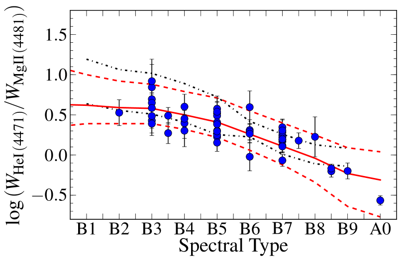
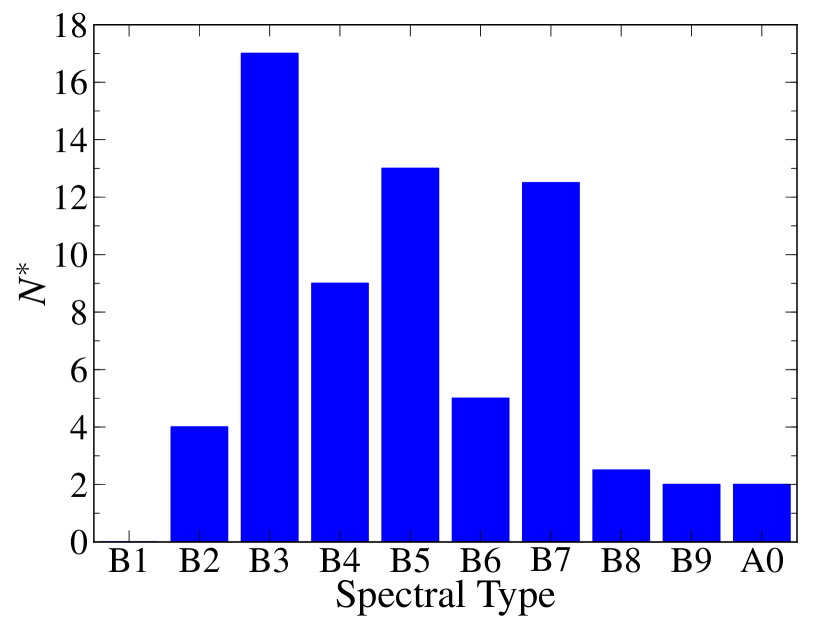
Figure 4: (a): Correlation between spectral type and the logarithm of the equivalent width ratio, W(He I $\lambda 4471$/Mg II $\lambda 4481$. Our sample is compared to an interpolation of the high-resolution data from Chauville et al. (2001): the black dotted curves mark the 1$\sigma$ confidence limits. Dashed red curves, instead, represent the 1$\sigma$ confidence limits obtained from repeated measures of equivalent-width ratios from appropriately chosen model atmospheres, with random noise added that matches S/N = 40. The blue circles are the values obtained for our sample. (b): The histogram of spectral sub-types in the CBe sample.

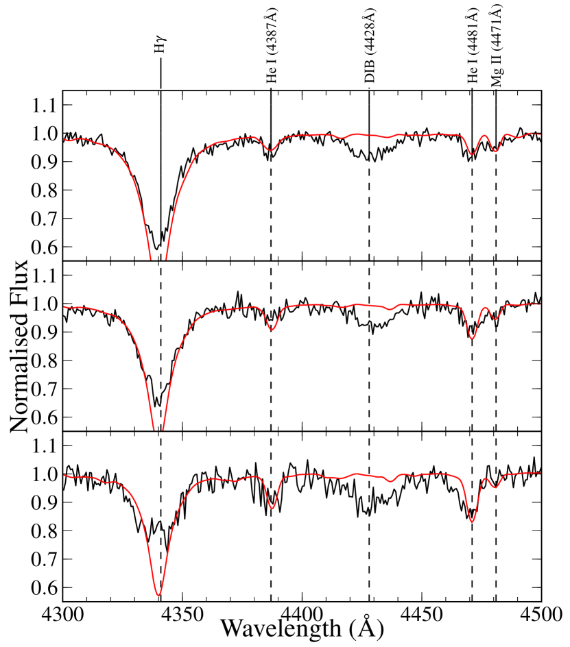
Figure 5: Examples of spectral type assignments based on three spectra with different $S/N$ ratio. From top to bottom, #41 (B7, $S/N=64)$, #65 (B5, $S/N=48)$, #50 (B3, $S/N=34)$. The observed spectra are in black while the preferred Munari et al. (2005) models are in red. The models have been rebinned to match that of the observations.

Where ${\rm H}\alpha$ was present in the wavelength range observed, it was always seen in emission. In the higher resolution NOT data, missing the red part of the spectrum, we generally found the $\rm{H}\beta$ line to be either inverted or partially filled in. This means that caution must be exercised in allowing the Balmer line profiles to inform the classification of a star’s spectrum.

Spectral types were first determined, by direct comparison both with spectral-type standards that we acquired during each observing run and also with templates taken from the INDO-US library (Valdes et al., 2004). The latter needed to be degraded in spectral resolution from the original $\Delta\lambda=1\,\rm{\AA}$ to match that of our data. Nearly all stars in the reduced sample of 67 were B stars exhibiting He I absorption, with only one or two crossing the boundary to A-type. No star showed He II, ruling out any as O-type. Our assignments were guided by the criteria to be found in Jaschek & Jaschek (1987), Gray & Corbally (2009) and Didelon (1982). The last of these usefully supplies quantitative measures of equivalent width variation with spectral type and luminosity class. Our list of key absorption lines for spectral type determination is:

• B-type: He I lines at $\lambda\lambda 4009$-$4026\,\rm{\AA}$, $\lambda\lambda 4121$-$4144\,\rm{\AA}$ and $\lambda\lambda\,4387$-$4471\rm{\AA}$ compared to the Mg II $\lambda 4481\,\rm{\AA}$;

• A-type: Ca II K and Mg II. The absence of He I.

How well fainter features can be detected depends on the specifics of the achieved S/N ratio and the spectral resolution – and the first of these depends in turn on how much interstellar extinction is present. Because the reddening is significant, it is generally the case that our classifications of the B stars depend heavily on the relative strengths of the He I $\lambda 4471$ and Mg II $\lambda 4481$ features – a good $T_{\rm{eff}}$ indicator, with little sensitivity to $\log{g}$ within classes V-III – rather than on shorter wavelength lines. As young, thin-disc objects, CBe stars are unlikely to present with distinctive blue spectra indicating significant metallicity variation, even to quite large heliocentric distances. So we make no attempt at this stage to treat metallicity as a detectable variable.

Furthermore, in CBe stars, the above mentioned transitions can be affected to differing extents by infilling line emission or continuum veiling due to the presence of ionised circumstellar discs, while in faster rotators, line blending can also be an issue. These factors raise challenges to typing methods dependent on main sequence (MS) templates. To overcome these problems, line equivalent widths ratios should also be brought into consideration, as these suffer less modification.

As a way of refining our spectral typing, where possible, we measured the absorption equivalent-width ratio $W_{\lambda 4471}/W_{\lambda 4481}$, via simple gaussian fitting with the STARLINK/DIPSO tool, and compared it with data from Chauville et al. (2001) and model atmospheres, in Fig. 4. The model atmosphere predictions include simulated noise, corresponding to S/N = 40. The precision of the typing, as judged by eye, is to $\pm$ one sub-type for all but the lowest quartile in S/N ratio (S/N $<$ 35) where it approaches $\pm$2 sub-types (these objects have generally larger uncertainties, $\Delta(\log{W_{\lambda 4471}/W_{\lambda 4481}})\gtrsim 0.30$, and are not plotted in Fig. 4). Noisy spectra are subject to a dual bias, depending on the actual value of the line ratio. Early-B types, when the Mg II line is weaker compared to the He I line, can appear earlier in type due to noise and, vice versa, a spectrum may be classified as a later type when the Mg II line is stronger than the He I line. In Fig. 4 the distribution of spectral types in the sample is shown: most are in fact proposed to be mid B stars.

We show in Fig. 5 some examples of our spectra within the 4300–4500 Å window compared with MS model atmospheres appropriate to the chosen MS spectral sub-type.

Luminosity class, for late-B and A stars, is in principle well-determined from the appearance of the Balmer lines (particularly the wings). For B sub-types earlier than B4, Gray & Corbally (2009) cite relative strengths of O II and Si II-IV absorption lines compared with H I and He I ones as luminosity-sensitive also. Assigning the right luminosity class is much more difficult than assigning spectral sub-type since emission in the Balmer series interferes with our view of the Balmer line profiles for many of our objects. Furthermore the combination of S/N ratio and moderate spectral resolution reduces the possibility to classify using the Balmer-line wings and renders the weaker O and Si gravity-sensitive transitions undetectable. An evaluation of the class III-V uncertainty and its impact on the distance determination will be discussed in Section 4.2 and 5.1.1.

The spectral types assigned to the observed stars are set out in Table 3 where, for the moment, the luminosity class is left unassigned.

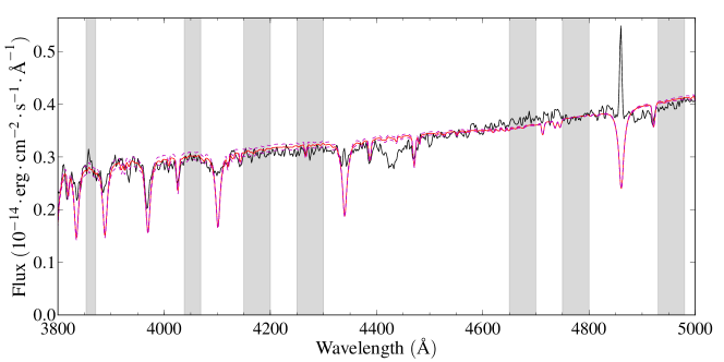
Figure 6: Example of a reddening measurement based on a blue spectrum. The INT spectrum of object #16 (black line) is shown along with the model atmosphere for $T_{\rm{eff}}=17000K$, reddened according to the best fitting colour excess ($E(B-V)_{{\rm S}}=1.27\pm 0.04$). The reddened model is drawn in red, with its 1-$\sigma$ error bounds shown as purple dashed lines. The shaded vertical strips pick out the continuum intervals used in the fitting procedure. The normalisation applied in this instance is at $\lambda\,4775\rm{\AA}$. Note that the poor agreement between the template Balmer line profiles and those of the star is due to infilling line emission.

3.2 Reddenings

Two methods are used to measure the reddening of each star in the sample. The first, our primary method that we deploy in the later parts of this study, is spectrophotometric and should be very sensitive since we access the blue part of the spectrum (3800–5000 Å), for all the objects. The second is essentially photometric, in that it makes use of the IPHAS $(r-i)$ colour but requires knowledge of spectral type (supplied by the spectroscopy). Given the presence of circumstellar excess emission, which is wavelength dependent, we expect to see a difference between the two determinations, in the sense that the photometric value is greater. We compute this second reddening to see if this expectation is borne out.

3.2.1 Reddening estimation: spectroscopic method

A least-squares fitting method was applied as follows.

First, we map the spectral sub-types of Section 3.1 onto an approximate $T_{\rm{eff}}$ scale, using Kenyon & Hartmann (1995) for main sequence stars (see Table 4). Then, the basic idea of the fit is to compare each observed spectrum with the corresponding solar-abundance model for the appropriate $T_{\rm{eff}}$, with $\log(g)=4.0$, taken from the Munari et al. (2005) library, as it is increasingly reddened – thereby seeking out the minimum reduced $\chi^{2}$. Numerical experiments show that the treatment of all objects as class V stars, when they may be more luminous class IV or III stars, introduces negligible error compared to all other terms in the error budget (see below).

So that the fitting is sensitive only to the overall slope of the observed SED compared with its theoretical value and not to the details of individual lines, the fits are carried out within carefully chosen spectral intervals that are free of structure due to deep absorption lines/bands (mainly the Balmer lines and DIBs). In effect we degrade both observation and model atmosphere to a number of ’line-free’ narrow bands falling in the range $\lambda\lambda 3800$ – $5000$ Å. Flux is averaged in each of these fit intervals and weighted according to the measured noise. In the fitting software, the reference model is progressively reddened, raising $E(B-V)_{{\rm S}}$ by 0.01 mag at each step, and the quality of fit to the observed spectrum is appraised by calculating $\chi^{2}$. In this approach, the number of degrees of freedom, $\nu$, is the number of adopted spectral intervals less the number of free parameters – here the latter number is 1 (for the reddening). In practice, fits were performed for two different normalisations of the model atmosphere to the data at 4250 Å  and 4750 Å, with the final reddening being the average of the two slightly different outcomes.

The reddening law used in all cases is based on the formulation given in Fitzpatrick (1999) with $R_{V}=3.1$. The choice of $R_{V}$ to within a few tenths has little impact on the derived colour excess, as small changes in $R_{V}$ scarcely change the slope of the lav in the blue-visual range. Nevertheless it does affect the distance estimates as we will explain in Section 5. One example of the results of the fit process is displayed, along with the selected wavelength intervals used in the fits, in Fig. 6.

Errors on $E(B-V)_{{\rm S}}$ are determined graphically, by identifying the $\Delta\chi^{2}\leq 1$ range around the minimum. We find that these are typically $\pm 0.05$ magnitudes.

In principle a systematic error is introduced into the determination of $E(B-V)_{{\rm S}}$, if the spectral type and mapping onto a reference model atmosphere are incorrect. Since the Planck maximum in B and even early-A stars is in the ultraviolet, their SEDs are tending towards the Rayleigh-Jeans limit in the optical. As a consequence the spectral type uncertainty does not generate a large extra error in $E(B-V)_{{\rm S}}$. Experiments in which the adopted model atmosphere is altered by $\pm 1$ sub-type or uprated to luminosity class III, indicate a further error of up to $\pm 0.05$ mag in $E(B-V)_{{\rm S}}$. There is, in addition, a random component linked to the known SED/colour spread associated with any one spectral type: based on the Hipparcos dataset Houk et al. (1997) showed, for B8 – F3 stars, $\sigma(B-V)\sim 0.03$. In the error budget, therefore, the direct fit error is in average equal or larger than the other sources of uncertainty.

The measured spectroscopic reddenings, $E(B-V)_{\rm{S}}$, are listed in Table 3.

Table 4: Adopted class V $T_{\rm{eff}}$ scale, intrinsic colours and absolute magnitude scale. The $T_{\rm{eff}}$ values are from Kenyon & Hartmann (1995); the intrinsic colours are computed taking the average of Sale et al. (2009), Fabregat (priv. comm.), Kenyon & Hartmann (1995), Siess, Forestini, & Dougados (1997). The absolute $r$ magnitudes are conversions of the absolute $V$ magnitudes given by Zorec & Briot (1991). In the final two columns we give class IV and III absolute magnitudes obtained from the same source. Uncertainties on $Mr$ are $50\%$ of the absolute errors given by Zorec & Briot (1991), which more closely resemble the standard deviations at each sub-type than the full range specified by Zorec & Briot (1991).

	dwarfs			subgiants	giants
SpT	$T_{\rm{eff}}$	$(r-i)_{\rm{o}}$	$\rm{M}_{r}$	$\rm{M}_{r}$	$\rm{M}_{r}$
	(K)	(mag)	(mag)	(mag)	(mag)
B0	30000	$-0.17$	$-3.40\pm 0.30$	$-3.70\pm 0.25$	$-4.20\pm 0.35$
B1	25400	$-0.15$	$-2.80\pm 0.30$	$-3.10\pm 0.20$	$-3.70\pm 0.35$
B2	22000	$-0.13$	$-2.10\pm 0.35$	$-2.50\pm 0.30$	$-3.30\pm 0.45$
B3	18700	$-0.12$	$-1.55\pm 0.25$	$-2.00\pm 0.20$	$-2.85\pm 0.50$
B4	17000	$-0.09$	$-1.15\pm 0.20$	$-1.65\pm 0.20$	$-2.45\pm 0.55$
B5	15400	$-0.08$	$-0.70\pm 0.20$	$-1.20\pm 0.25$	$-2.30\pm 0.55$
B6	14000	$-0.07$	$-0.30\pm 0.20$	$-0.75\pm 0.25$	$-1.90\pm 0.55$
B7	13000	$-0.06$	$-0.10\pm 0.20$	$-0.50\pm 0.25$	$-1.60\pm 0.50$
B8	11900	$-0.04$	$0.20\pm 0.25$	$-0.30\pm 0.25$	$-1.30\pm 0.50$
B9	10500	$-0.02$	$0.60\pm 0.25$	$0.10\pm 0.30$	$-0.90\pm 0.60$
A0	9520	$0.00$	$1.00\pm 0.25$	$0.50\pm 0.30$	$-0.50\pm 0.60$

Table 3: Spectral parameters of the 67 CBe stars, as derived in Section 3. Columns are in the following order: ID number; spectral type; S/N at $\lambda\,4500$ Å; measured colour excess; H$\alpha$ emission-corrected $(r-i)_{\rm{c}}$ colours; photometric colour excess; absorption-corrected ${\rm H}\alpha$ equivalent width; disc fraction from the scaling relation, equation (5). The final columns lists the spectroscopic interstellar reddening $E(B-V)_{\rm{(S,c)}}$, after correction for the circumstellar excess, and the asymptotic value of $E(B-V)$ for the sight-line from SFD98.

#	SpT	S/N	$E(B-V)_{\rm{S}}$	$(r-i)_{\rm{c}}$	$E(B-V)_{\rm{P}}$	$EW({\rm H}\alpha)$	$f_{\rm{D}}$	$E(B-V)_{\rm{(S,c)}}$	$E(B-V)_{\rm{SFD98}}$
			(mag)	(mag)	(mag)	(Å)		(mag)	(mag)
$1$	B5	47	$1.40\pm 0.08$	$0.87$	$1.37\pm 0.09$	$-25.4\pm 1.1$	$0.08$	$1.36\pm 0.08$	$1.51$
$2$	B7	67	$0.66\pm 0.07$	$0.35$	$0.60\pm 0.05$	$-12.6\pm 0.9$	$0.04$	$0.64\pm 0.07$	$1.58$
$3$	B3	40	$1.60\pm 0.08$	$1.00$	$1.62\pm 0.10$	$-34.6\pm 0.8$	$0.12$	$1.54\pm 0.08$	$1.83$
$4$	A0	29	$1.02\pm 0.09$	$0.77$	$1.12\pm 0.08$	$-22.5\pm 1.3$	$0.08$	$0.98\pm 0.09$	$1.78$
$5$	B2	44	$1.14\pm 0.08$	$0.73$	$1.25\pm 0.08$	$-44.7\pm 0.9$	$0.15$	$1.07\pm 0.08$	$1.55$
$6$	B3	25	$1.38\pm 0.10$	$0.91$	$1.49\pm 0.09$	$-25.8\pm 1.1$	$0.09$	$1.34\pm 0.10$	$1.51$
$7$	B7	35	$0.84\pm 0.07$	$0.51$	$0.82\pm 0.06$	$-17.5\pm 1.2$	$0.06$	$0.81\pm 0.07$	$1.51$
$8$	B3	31	$1.12\pm 0.07$	$0.63$	$1.09\pm 0.07$	$-30.2\pm 1.4$	$0.10$	$1.07\pm 0.07$	$1.28$
$9$	B5	37	$0.94\pm 0.08$	$0.56$	$0.93\pm 0.06$	$-17.6\pm 1.0$	$0.06$	$0.91\pm 0.08$	$1.60$
$10$	B7	40	$1.10\pm 0.08$	$0.68$	$1.08\pm 0.07$	$-33.8\pm 0.8$	$0.11$	$1.05\pm 0.08$	$1.66$
$11$	B2-3	55	$0.96\pm 0.08$	$0.65$	$1.12\pm 0.07$	$-48.5\pm 0.9$	$0.16$	$0.88\pm 0.08$	$1.07$
$12$	B5	49	$0.86\pm 0.09$	$0.51$	$0.85\pm 0.06$	$-19.6\pm 1.2$	$0.07$	$0.83\pm 0.09$	$1.15$
$13$	B5	81	$0.66\pm 0.08$	$0.38$	$0.67\pm 0.05$	$-13.6\pm 1.0$	$0.05$	$0.64\pm 0.08$	$1.02$
$14$	B4	61	$1.14\pm 0.08$	$0.75$	$1.22\pm 0.08$	$-31.4\pm 1.3$	$0.10$	$1.09\pm 0.08$	$1.37$
$15$	B5	87	$1.10\pm 0.07$	$0.74$	$1.18\pm 0.08$	$-25.4\pm 0.8$	$0.08$	$1.06\pm 0.07$	$1.66$
$16$	B3	67	$1.27\pm 0.08$	$0.88$	$1.45\pm 0.09$	$-29.1\pm 0.8$	$0.10$	$1.22\pm 0.08$	$1.91$
$17$	B3	38	$1.53\pm 0.08$	$1.01$	$1.64\pm 0.10$	$-91.6\pm 0.9$	$0.31$	$1.36\pm 0.08$	$1.47$
$18$	B4	54	$1.07\pm 0.08$	$0.74$	$1.20\pm 0.08$	$-48.1\pm 1.0$	$0.16$	$0.99\pm 0.08$	$1.39$
$19$	B6	28	$1.14\pm 0.07$	$0.64$	$1.03\pm 0.07$	$-23.8\pm 1.2$	$0.08$	$1.10\pm 0.07$	$1.19$
$20$	B3	51	$1.40\pm 0.08$	$0.99$	$1.61\pm 0.10$	$-72.6\pm 0.8$	$0.24$	$1.28\pm 0.08$	$1.90$
$21$	B5	30	$1.40\pm 0.09$	$0.87$	$1.38\pm 0.09$	$-43.8\pm 1.3$	$0.15$	$1.33\pm 0.09$	$2.39$
$22$	B4	41	$1.33\pm 0.07$	$0.92$	$1.47\pm 0.09$	$-27.3\pm 1.0$	$0.09$	$1.29\pm 0.07$	$1.40$
$23$	B7	48	$1.08\pm 0.09$	$0.77$	$1.20\pm 0.08$	$-50.0\pm 1.0$	$0.17$	$1.00\pm 0.09$	$1.39$
$24$	B3	54	$1.36\pm 0.07$	$0.89$	$1.46\pm 0.09$	$-32.2\pm 0.8$	$0.11$	$1.31\pm 0.07$	$1.96$
$25$	B5	79	$0.86\pm 0.07$	$0.55$	$0.92\pm 0.06$	$-25.0\pm 0.8$	$0.08$	$0.82\pm 0.07$	$1.19$
$26$	B3	33	$1.18\pm 0.09$	$0.85$	$1.41\pm 0.09$	$-99.4\pm 1.1$	$0.33$	$1.00\pm 0.09$	$1.37$
$27$	B5	44	$1.08\pm 0.07$	$0.67$	$1.09\pm 0.07$	$-19.6\pm 1.0$	$0.07$	$1.05\pm 0.07$	$1.30$
$28$	B7	50	$0.83\pm 0.08$	$0.48$	$0.78\pm 0.06$	$-20.0\pm 0.9$	$0.07$	$0.80\pm 0.08$	$1.12$
$29$	B7	69	$0.80\pm 0.07$	$0.50$	$0.81\pm 0.06$	$-19.4\pm 0.9$	$0.06$	$0.77\pm 0.07$	$1.42$
$30$	B4	45	$0.78\pm 0.07$	$0.45$	$0.78\pm 0.06$	$-5.3\pm 1.2$	$0.02$	$0.77\pm 0.07$	$0.97$
$31$	B3	56	$1.28\pm 0.07$	$0.89$	$1.46\pm 0.09$	$-24.5\pm 0.9$	$0.08$	$1.24\pm 0.07$	$1.74$
$32$	B6	66	$1.01\pm 0.08$	$0.54$	$0.88\pm 0.06$	$-25.6\pm 0.9$	$0.09$	$0.97\pm 0.08$	$0.93$
$33$	B8-9	77	$0.88\pm 0.07$	$0.58$	$0.88\pm 0.07$	$-14.4\pm 0.7$	$0.05$	$0.86\pm 0.07$	$1.02$
$34$	B3	47	$0.70\pm 0.08$	$0.49$	$0.88\pm 0.06$	$-36.9\pm 0.9$	$0.12$	$0.64\pm 0.08$	$1.18$
$35$	B2-3	47	$0.93\pm 0.08$	$0.58$	$1.02\pm 0.07$	$-56.5\pm 1.1$	$0.19$	$0.84\pm 0.08$	$1.09$
$36$	B4	37	$1.53\pm 0.10$	$1.11$	$1.74\pm 0.11$	$-59.0\pm 1.0$	$0.20$	$1.43\pm 0.10$	$2.06$
$37$	B6	51	$0.92\pm 0.08$	$0.61$	$0.98\pm 0.07$	$-18.5\pm 0.9$	$0.06$	$0.89\pm 0.08$	$1.19$
$38$	B5	22	$0.90\pm 0.15$	$0.68$	$1.10\pm 0.07$	$-21.0\pm 1.3$	$0.07$	$0.87\pm 0.15$	$1.61$
$39$	B4	27	$0.96\pm 0.12$	$0.75$	$1.22\pm 0.08$	$-82.4\pm 1.1$	$0.27$	$0.82\pm 0.12$	$0.93$
$*40$	B2	52	$1.04\pm 0.07$	$0.67$	$1.16\pm 0.07$	$-13.2\pm 1.5$	$0.04$	$1.02\pm 0.07$	$0.32$
$*41$	B7	64	$1.02\pm 0.07$	$0.57$	$0.92\pm 0.06$	$-19.2\pm 1.6$	$0.06$	$0.99\pm 0.07$	$0.95$
$*42$	B2	22	$1.47\pm 0.08$	$1.00$	$1.63\pm 0.10$	$-70.3\pm 2.2$	$0.23$	$1.36\pm 0.08$	$0.94$
$*43$	B6	48	$0.82\pm 0.07$	$0.44$	$0.74\pm 0.05$			$0.82\pm 0.07$	$0.68$
$*44$	B5	51	$0.79\pm 0.07$	$0.56$	$0.93\pm 0.06$	$-9.6\pm 2.6$	$0.03$	$0.78\pm 0.07$	$0.85$
$45$	B3	103	$1.14\pm 0.07$	$0.64$	$1.10\pm 0.07$	$-19.2\pm 0.8$	$0.06$	$1.11\pm 0.07$	$1.51$
$*46$	B9	40	$0.84\pm 0.07$	$0.57$	$0.86\pm 0.07$	$-16.8\pm 1.6$	$0.06$	$0.81\pm 0.07$	$1.19$
$*47$	B3	36	$1.65\pm 0.07$	$1.13$	$1.81\pm 0.11$	$-42.2\pm 1.2$	$0.14$	$1.58\pm 0.07$	$1.98$
$*48$	B8	22	$1.15\pm 0.10$	$0.74$	$1.13\pm 0.08$			$1.15\pm 0.10$	$1.23$
$*49$	A0	43	$0.74\pm 0.07$	$0.44$	$0.64\pm 0.05$	$-26.5\pm 3.3$	$0.09$	$0.70\pm 0.07$	$0.72$
$*50$	B3	34	$1.00\pm 0.08$	$0.75$	$1.26\pm 0.08$	$-47.0\pm 2.0$	$0.16$	$0.92\pm 0.08$	$1.26$
$*51$	B8-9	63	$0.73\pm 0.07$	$0.41$	$0.63\pm 0.06$	$-12.3\pm 1.3$	$0.04$	$0.71\pm 0.07$	$0.78$
$*52$	B7	40	$0.90\pm 0.08$	$0.60$	$0.96\pm 0.07$	$-18.0\pm 2.7$	$0.06$	$0.87\pm 0.08$	$0.98$
$*53$	B7	45	$1.11\pm 0.07$	$0.67$	$1.05\pm 0.07$	$-41.6\pm 1.7$	$0.14$	$1.04\pm 0.07$	$1.47$
$*54$	B3	51	$0.85\pm 0.07$	$0.48$	$0.86\pm 0.06$	$-26.8\pm 2.0$	$0.09$	$0.81\pm 0.07$	$1.12$
$*55$	B3-4	28	$1.04\pm 0.08$	$0.72$	$1.19\pm 0.08$	$-37.8\pm 2.0$	$0.13$	$0.98\pm 0.08$	$1.22$
Note: ∗ NOT/ALFOSC observations, for which ${\rm H}\alpha$ equivalent widths were measured from FLWO-1.5m/FAST spectra when available.

Table 4: continued

#	SpT	S/N	$E(B-V)_{\rm{S}}$	$(r-i)_{\rm{c}}$	$E(B-V)_{\rm{P}}$	$EW({\rm H}\alpha)$	$f_{\rm{D}}$	$E(B-V)_{\rm{(S,c)}}$	$E(B-V)_{\rm{SFD98}}$
			(mag)	(mag)	(mag)	(Å)		(mag)	(mag)
$*56$	B7	45	$1.02\pm 0.07$	$0.69$	$1.09\pm 0.07$	$-47.4\pm 1.6$	$0.16$	$0.94\pm 0.07$	$1.72$
$*57$	B7-8	52	$1.00\pm 0.08$	$0.70$	$1.09\pm 0.08$			$1.00\pm 0.08$	$1.36$
$*58$	B3	44	$0.72\pm 0.07$	$0.36$	$0.70\pm 0.05$	$-31.4\pm 1.2$	$0.10$	$0.67\pm 0.07$	$0.90$
$*59$	B5	44	$0.78\pm 0.08$	$0.47$	$0.80\pm 0.05$	$-52.2\pm 1.8$	$0.17$	$0.70\pm 0.08$	$1.24$
$*60$	B3-4	36	$0.82\pm 0.08$	$0.39$	$0.72\pm 0.06$	$-31.2\pm 3.1$	$0.10$	$0.77\pm 0.08$	$1.24$
$*61$	B7	51	$0.74\pm 0.08$	$0.43$	$0.71\pm 0.05$	$-11.4\pm 1.6$	$0.04$	$0.72\pm 0.08$	$0.81$
$*62$	B6	26	$1.23\pm 0.10$	$0.77$	$1.21\pm 0.08$	$-16.7\pm 1.6$	$0.06$	$1.20\pm 0.10$	$1.62$
$*63$	B7	58	$0.89\pm 0.07$	$0.52$	$0.84\pm 0.06$			$0.89\pm 0.07$	$1.67$
$*64$	B5	37	$1.25\pm 0.09$	$0.81$	$1.29\pm 0.08$	$-17.0\pm 2.1$	$0.06$	$1.22\pm 0.09$	$1.32$
$*65$	B5	48	$0.98\pm 0.07$	$0.56$	$0.92\pm 0.06$	$-31.4\pm 1.4$	$0.10$	$0.93\pm 0.07$	$1.55$
$*66$	B4	31	$1.10\pm 0.08$	$0.64$	$1.05\pm 0.07$	$-25.5\pm 1.4$	$0.08$	$1.06\pm 0.08$	$1.72$
$67$	B4	35	$1.14\pm 0.11$	$0.81$	$1.31\pm 0.09$	$-18.2\pm 0.9$	$0.06$	$1.11\pm 0.11$	$1.51$
Note: ∗ NOT/ALFOSC observations, for which ${\rm H}\alpha$ equivalent widths were measured from FLWO-1.5m/FAST spectra when available.

3.2.2 Reddening estimation: photometric method

IPHAS photometry provides an observed $(r-i)$ colour that can be used in conjunction with the now known spectral type to give another reddening estimate. The procedure we adopted to do this has three steps:

1. The observed $(r-i)$ colour is corrected to zero ${\rm H}\alpha$ emission, by reference to the synthetic tracks given in Drew et al. (Table 4, 2005). This is a small correction, in the range 0.01 – 0.05 magnitudes. Corrected colours, $(r-i)_{\rm{c}}$, are in table 3.

2. The colour excess for each object is then:

   $$E(r-i)=(r-i)_{\rm{c}}-(r-i)_{\rm{o}},$$ (1)

   where $(r-i)_{\rm{o}}$ is the intrinsic colour, consistent with the spectral type assigned in Section 3.1. The adopted intrinsic colours are set out in Table 4.

3. The $(B-V)$ colour excess is then computed as:

   $$E(B-V)_{\rm{P}}=E(r-i)/0.69,$$ (2)

   adopting the same $R_{v}=3.1$ reddening curve as applied in Section 3.2.1.

Random photometric uncertainties in $r$ and $i$ for these relatively bright objects are small – not exceeding 0.01. Further uncertainties to include are:

1. the spread in intrinsic colour, as commented on above in Section 3.2.1.

2. the uncertainty originating from the $\pm 1$ sub-type error in the spectral-typing. Across the B class this averages to $\pm 0.02$ mag. As for the SED fitting, an uncertainty on the luminosity classes would introduce a small $\pm 0.01$ mag error.

Photometric reddenings, $E(B-V)_{\rm{P}}$, are also recorded in Table 3.

Table 5: Circumstellar colour excess and $r$ magnitude corrections for a given spectral type and disc contribution to the total flux.

		$f_{\rm{D}}$ = 0.05		$f_{\rm{D}}$ = 0.10		$f_{\rm{D}}$ = 0.20		$f_{\rm{D}}$ = 0.30
SpT	$T_{e}(K)$	$E^{cs}(B-V)_{\rm{S}}$	$\Delta r$	$E^{cs}(B-V)_{\rm{S}}$	$\Delta r$	$E^{cs}(B-V)_{\rm{S}}$	$\Delta r$	$E^{cs}(B-V)_{\rm{S}}$	$\Delta r$
B1	18000	0.023	0.082	0.046	0.166	0.098	0.344	0.156	0.516
B3	13200	0.022	0.085	0.048	0.173	0.103	0.357	0.164	0.534
B5	9300	0.024	0.089	0.049	0.180	0.105	0.369	0.169	0.552
B7	7800	0.024	0.093	0.049	0.188	0.105	0.385	0.170	0.573
A0	5700	0.023	0.104	0.047	0.209	0.103	0.424	0.168	0.627

3.3 Correction for CBe circumstellar continuum emission

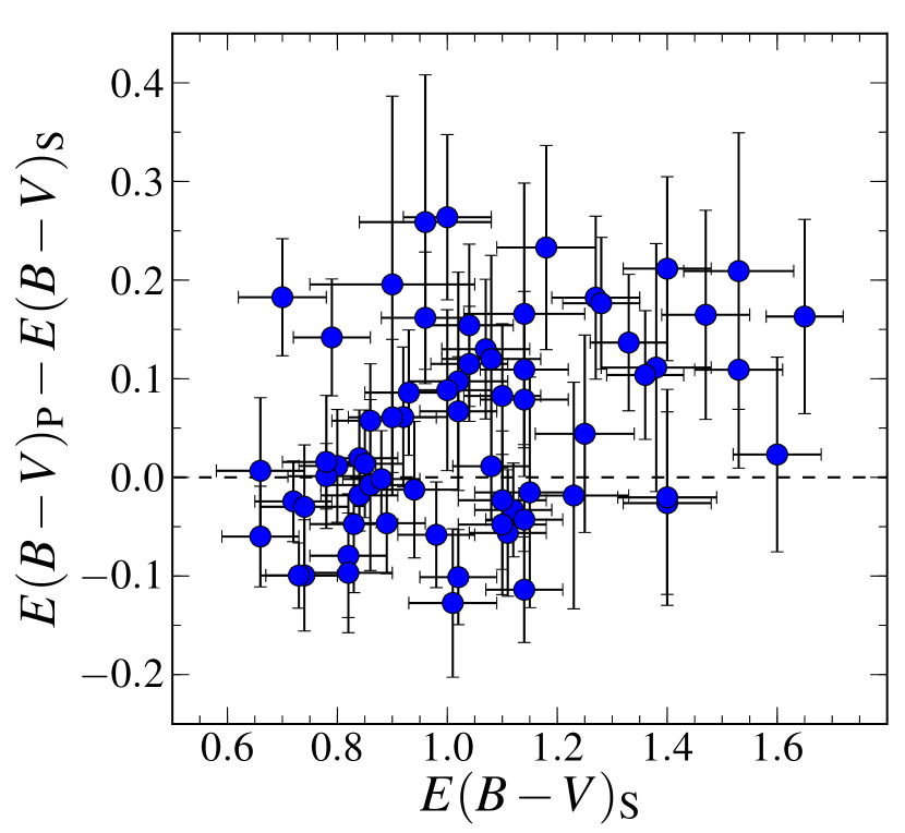
Figure 7: The difference between the two colour excess measurements, $E(B-V)_{\rm{P}}-E(B-V)_{\rm{S}}$ is plotted as a function of the spectroscopic colour excess, $E(B-V)_{\rm{S}}$. The data points are scattered with a bias to positive values, as expected, due to the reddening effect associated with the circumstellar-disc emission present in these stars.

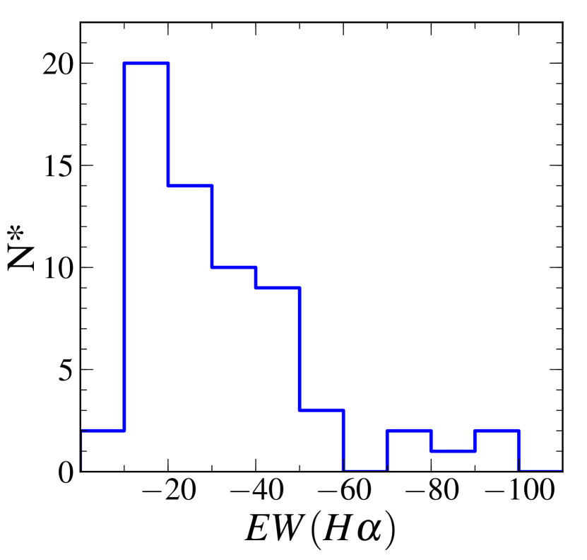
Figure 8: The distribution of H$\alpha$ equivalent widths ($EW({\rm H}\alpha)$). The median of the distribution falls at $\approx-26$ Å  and all but 5 of the 67 stars have $EW({\rm H}\alpha)\leq-60$ Å.

CBe stars are affected by excess emission which slightly alters the optical SED and induces an overestimate of the colour excess, $E(B-V)$, if not taken into account. Following earlier notation (Dachs, Kiehling, & Engels, 1988), this component can be treated as additive to the interstellar value as in:

$$E(B-V)=E^{is}(B-V)+E^{cs}(B-V),$$ (3)

where $E^{is}(B-V)$ is the interstellar reddening and $E^{cs}(B-V)$ is the circumstellar contribution to the total colour excess.

Kaiser (1989) and, more recently Carciofi & Bjorkman (2006), have demonstrated that the continuum excess, accounted for by $E^{cs}(B-V)$, can be attributed to an optically-thin free-free and recombination free-bound continuum . It is evident from this work that the wavelength dependence of the disc continuum is such that the red spectrum includes more disc light than the blue. Dachs, Kiehling, & Engels (1988) specifically investigated the correlation between $EW({\rm H}\alpha)$ and $E^{cs}(B-V)$ and presented evidence that the former correlates with the latter and also with the fraction of the total emission that can be attributed to the circumstellar disc. By analysing a sample of B0–B3 stars mainly, they found the following dependencies on ${\rm H}\alpha$ emission equivalent width:

$$E^{cs}(B-V) \approx 0.02\cdot\frac{EW({\rm H}\alpha)}{-10\rm{\AA}}$$ (4)

$$f_{\rm D}=\frac{F_{\rm D}}{F_{{\rm D}}+F^{*}} \approx 0.1\cdot\frac{EW({\rm H}\alpha)}{-30\rm{\AA}},$$ (5)

where $f_{\rm{D}}=F_{\rm{D}}/(F_{\rm{D}}+F^{*})$ is the fraction of flux emitted by the disc compared to the total flux, at $\lambda\,5500\rm{\AA}$.

First we confirm that our sample of objects presents the expected evidence of a continuum excess that affects the red-optical more than the blue-optical. Fig. 7 compares the two reddening measurements we have obtained for all members of the sample. In it, we notice a systematic overestimate of $E(B-V)_{\rm{P}}$ with respect to $E(B-V)_{\rm{S}}$, which ties in with the description given by Kaiser (1989). Where $E(B-V)_{\rm P}$ is less than $E(B-V)_{\rm S}$ it is never so negative that it may not be viewed as consistent with the two measures being equal to within the errors. This is encouraging in the sense that this outcome would not be guaranteed if the sample contained CBe stars prone to marked variability.

A new feature of our sample compared to that of Dachs, Kiehling, & Engels (1988) is that it includes 5 objects with $EW({\rm H}\alpha)\leq-60\rm{\AA}$ (see Fig. 8), that therefore lie beyond the range over which the correlations contained in equations (4) and (5) were established.

Our method for estimating the circumstellar colour excess begins with equation (5), delivering the disc fraction, $f_{\rm{D}}$. We do not simply apply equation (4) for the reason that it was constructed to provide correction to reddenings measured directly across the $B$ to $V$ range (roughly 4000 — 6000 Å). The spectrophotometric reddening estimates obtained here are based on the blue range only, stopping at 5000 Å, where the contaminating circumstellar disc continuum will be less than the mean for the $B$ to $V$ range.

We have computed some simple models that enable an appropriate scaling down of this correction. It is assumed that the disc is optically thin at least in the Paschen continuum, emitting free-free and free-bound continuum emission from a fully ionised hydrogen envelope (Dachs, Kiehling, & Engels, 1988; Kaiser, 1989; Carciofi & Bjorkman, 2006). Our parametrisation is similar to that of Kaiser (1989), in that we maintain the same definition of $f_{\rm{D}}$. Our simulations cover the range of spectral types present in our sample (B1 to A0), and disc fractions are varied from zero to a maximum of 0.45. A significant difference with respect to earlier treatments is that we adopt a scaling of the electron temperature in the circumstellar disc such that $T_{e}=0.6\cdot T_{\rm{eff}}$: this has been shown to be a good approximation by Carciofi & Bjorkman (2006) (see also Drew, 1989). The electron density is set at the suitably high, representative value, $N_{e}=10^{12}\,\rm{cm}^{-3}$ (Dachs, Kiehling, & Engels, 1988; Dachs, Rohe, & Loose, 1990).

On this basis we generate the circumstellar continuum emission and add it to the Munari et al. (2005) model atmospheres, scaling it as required at $\lambda\,5500\rm{\AA}$. The correction, $E^{cs}(B-V)_{\rm{S}}$ can then be determined by ’dereddening’ the resultant total spectrum to match the model atmosphere alone. This is carried out within the wavelength range $\lambda\lambda\,3800\rm{\AA}$ – $5000\rm{\AA}$, paralleling the procedure applied to the observed spectra (Section 3.2.1).

In Table 5 we provide a representative grid of spectral types and corresponding $E^{cs}(B-V)_{\rm{S}}$, for a given disc contribution ($f_{\rm{D}}$) to the total emitted flux. Later, the $r$ magnitudes of our sample will also need to be corrected to remove the circumstellar disc contribution. Our simulations provide this correction, $\Delta r$, as well. These are also given in Table 5. We find that the $r$ magnitudes of our sample will be brighter, due to circumstellar emission, by amounts ranging from zero up to 0.5 in the most extreme cases.

Since CBe stars are known to be erratic variables (i.e. Zorec & Briot, 1991; Porter & Rivinius, 2003; Jones, Tycner, & Smith, 2011), we take care to determine $f_{\rm D}$ from either observations of the H$\alpha$ line that are simultaneous with our blue spectroscopy (available with all our INT data), or from a well-validated proxy in the case of the NOT spectra without coverage of the H$\alpha$ region. The necessary proxy is provided by the FLWO-1.5m/FAST spectra in which we find that the H$\beta$ profile is a good match to that apparent in the NOT spectrum. Fortuitously there are good matches for all but 4 objects. We list the values of $f_{\rm D}$ obtained for each of our sample of stars in Table 3, where we also give the H$\alpha$ emission equivalent width on which it is based. This quantity is corrected for the underlying absorption, according to spectral type (see tabulation in Jaschek & Jaschek, 1987). The error on $f_{\rm{D}}$ mainly reflects the scatter in the original empirical relation due to Dachs, Kiehling, & Engels (1988). We estimate this to be $\pm 0.02$ dex, and propagate it through into the $E^{cs}(B-V)$ error.

The final $E^{is}(B-V)$ is thus obtained by subtracting our tailored estimate of $E^{cs}(B-V)$ from $E(B-V)_{\rm S}$. This result is shown in the final column of Table 3. The distribution of final corrected reddenings is displayed in Fig. 9. It ranges between 0.6 – 1.5 mags. and the median $E(B-V)_{\rm{S,\,c}}$ is 0.98.

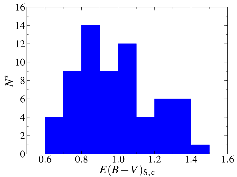
Figure 9: The distribution of reddenings corrected for circumstellar colour excess. The median of the distribution is found at $E(B-V)_{\rm{S,\,c}}=0.98$

4 Distance estimation

To set constraints on the distances to our objects, we first determine spectroscopic parallaxes adopting absolute magnitudes of both luminosity class V, IV and III. Secondly, we constrain the luminosity class of the CBe stars in the sample with help of IPHAS photometry of non-emission line stars that are seen along the corresponding sightline and share similar reddenings with each CBe star.

4.1 Distances from spectroscopic parallax

Spectroscopic parallax distances, $D_{\rm{SP}}$, are computed in the standard way, via the use of spectral types and reddenings that were determined in Section 3 and the absolute magnitudes listed in Table 4. Our magnitude scale is taken from Zorec & Briot (1991) from which we also obtain error estimates; if compared to others available in the literature (e.g Straizys & Kuriliene, 1981; Aller et al., 1982; Wegner, 2000) the Zorec & Briot scale furnishes slightly fainter magnitudes than some although they agree within the errors. We transformed their $V$-band absolute magnitudes into $r$ absolute magnitudes, using the intrinsic $(V-R_{C})$ colours for dwarfs supplied by Kenyon & Hartmann (1995), whilst noting that $R_{C}$ and $r$ magnitudes of B stars in the Vega system are close enough to identical for present purposes. Furthermore, the differences between dwarf and giant colours is small compared to all errors, permitting the use of MS colours in obtaining $M_{r}$ for B giants.

The observed $r$ magnitude needs to be corrected for the added flux due to circumstellar emission that makes the star look brighter than it would otherwise be (example values for the correction, $\Delta r$, appear in Table 5). The extinction in the $r$ band is given by $A_{r}=2.53\cdot E(B-V)_{\rm{(S,c)}}$, applying the same $R=3.1$ extinction law adopted in Section 3.2. The main contributions to the uncertainty in $D_{\rm{SP}}$ are the error in $E(B-V)_{\rm{(S,c)}}$ ($\sigma\sim 0.1$) and in $M_{r}$ (as specified in Table 4).

In Table 6 we list the input corrected magnitudes $r+\Delta r$ and $D_{\rm{SP}}$, computed both for luminosity class V, IV and III.

4.2 Constraining the luminosity class

In Section 3.1, it was noted that the spectra used for typing are not of the quality needed to pin down luminosity class. We now attempt to establish some constraints on this by exploiting a very general property of the IPHAS colour-colour plane, which permits disentangling of intrinsic colours and reddenings of ordinary MS stars. To do this, we adapt the methods of analysis described in Drew et al. (2008) and Sale et al. (2010), which focused on A-star selection, and in Sale et al. (2009), which presented a more general 3D extinction mapping algorithm. Essentially, for each CBe star, we pick out from IPHAS photometry fainter nearby non-emission line objects of similar reddening to see if, collectively, these putative lower main sequence companion objects favour a particular distance modulus, and hence – by implication – a particular luminosity class. By this means we choose between the class V, class IV and class III distance options listed in Table 6.

The method consists of the following steps and is illustrated by the two examples shown in Fig. 10:

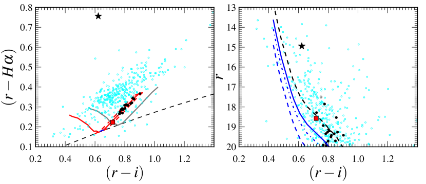
(a) # 11

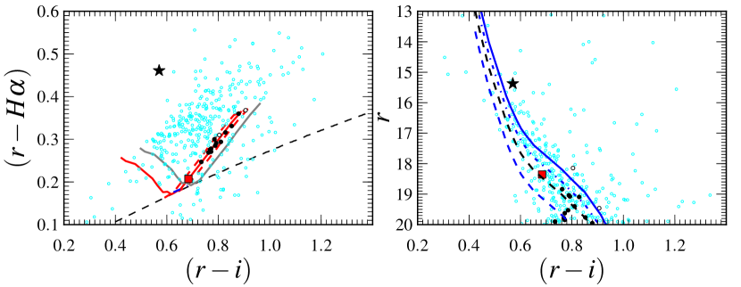
(b) # 52

Figure 10: Two examples of luminosity class assignment based on the IPHAS photometry of stars selected within a box of $10\times 10$ arcmin² centred on the CBe star. The top panel shows the data relevant to star # 11, while the bottom one pertains to star # 52. To the left, sightline colour-colour diagrams for stars with $r\leq 20$ are presented. The solid red curve in each case is the MS track, reddened by same amount as the CBe star. The red-dashed lines are the tracks for $E(B-V)_{{\rm S,c}}\pm 0.5\sigma$: stars falling between them are selected as stars of similar reddening – only those with $(r-H\alpha)$ colour consistent with their being A–F stars are retained (these are picked out in black). The CBe star itself is marked by the star symbol. The grey MS track also drawn is reddened at the line-of-sight SFD98 asymptotic colour excess. The dashed black curve is the early-A reddening line. The right hand panels present the colour-magnitude diagrams for the $10\times 10$ arcmin² selections. The reddened MS loci, computed for the distance moduli consistent with the CBe star as (i) class V, (ii) class IV, or (iii) class III are plotted respectively as solid, dash-dotted and dashed blue curves. The formal best-fit MS locus (reddened by the same amount as the CBe star) is plotted as a dashed black curve. Stars contributing to the fit are the black filled dots and the red squares (early A stars), while the unfilled black circles are stars excluded from the fit.

1. The photometry of all the stellar and probably-stellar point sources (morphology classification codes -1 and -2) with $r\leq 20$ is collected (cyan empty circles), within an on-sky box of $10\times 10$ arcmin² centred on each CBe star (black star in figure 10).

2. The MS track, reddened by the amount corresponding to $E(B-V)_{\rm{S,c}}$, is identified (plotted as the red solid curve in the left-hand panels of Fig. 10). This was produced by computing synthetic $(r,\,i,\,{\rm H}\alpha)$ photometry from a grid of (Munari et al., 2005) MS models, that were scaled to the Calspec model Vega spectrum.

3. All the point sources that fall within the reddening range, $E(B-V)_{\rm{S,c}}\pm 0.5\sigma$ (dashed red curves), and have the colours appropriate to early-A to late-F stars, are selected. The working assumption is that these stars, in sharing essentially the same reddening, are likely to be as far away as the CBe star.

   Table 6: Table of spectroscopic parallaxes of the CBe stars. Columns list: ID number; spectral type; Galactic coordinates; the observed $r$ magnitude corrected for circumstellar disc emission; $A_{r}$, computed from $E(B-V)_{\rm{(S,c)}}$; A/F fit approximate distances; spectro-photometric distances for luminosity classes V, IV and and III. In bold-face are distances that are associated to the preferred luminosity class, which is noted in the last column. The error on $D_{\rm{SP}}$ carries independent contributions from: photometric error, reddening error, disc emission uncertainty and the spread in absolute magnitude, as given in Table 4.

   						Distances
   #	SpT	$\ell$	$b$	$r+\Delta r$	$A_{r}$	A/F fit	$D_{\rm{SP,V}}$	$D_{\rm{SP,IV}}$	$D_{\rm{SP,III}}$	Likely
   		(deg)	(deg)	(mag)	(mag)	(kpc)	(kpc)	(kpc)	(kpc)	Class
   1	B5	120.04	1.64	$14.90\pm 0.04$	3.44	5.1	$2.7\pm 0.3$	$3.4\pm 0.5$	${\bf 5.6\pm 1.5}$	III
   2	B7	120.45	0.32	$14.14\pm 0.04$	1.62	2.9	${\bf 3.3\pm 0.4}$	$4.0\pm 0.6$	$6.6\pm 1.6$	V
   3	B3	121.09	3.99	$14.66\pm 0.03$	3.90	4.7	$2.9\pm 0.4$	$3.6\pm 0.5$	${\bf 5.2\pm 1.3}$	III
   4	A0	121.40	3.92	$16.12\pm 0.04$	2.48	3.7	${\bf 3.4\pm 0.5}$	$4.2\pm 0.7$	$6.7\pm 2.0$	V
   5	B2	121.76	2.43	$15.05\pm 0.03$	2.71	3.4	${\bf 7.8\pm 1.5}$	$9.4\pm 1.6$	$13.5\pm 3.1$	V
   6	B3	122.26	1.16	$15.78\pm 0.04$	3.39	7.0	$6.1\pm 1.0$	${\bf 7.7\pm 1.1}$	$11.1\pm 2.9$	IV
   7	B7	122.41	0.12	$14.98\pm 0.04$	2.05	3.0	${\bf 4.0\pm 0.5}$	$4.8\pm 0.7$	$8.0\pm 1.9$	V
   8	B3	122.79	0.72	$15.54\pm 0.04$	2.71	5.5	${\bf 7.5\pm 1.1}$	$9.4\pm 1.2$	$13.6\pm 3.3$	V
   9	B5	122.80	2.07	$14.26\pm 0.04$	2.30	3.1	${\bf 3.4\pm 0.5}$	$4.2\pm 0.6$	$7.0\pm 1.9$	V
   10	B7	122.83	2.69	$14.86\pm 0.04$	2.66	4.4	$2.9\pm 0.4$	${\bf 3.4\pm 0.5}$	$5.7\pm 1.4$	IV
   11	B2-3	123.29	0.23	$15.22\pm 0.04$	2.23	6.1	${\bf 9.2\pm 1.5}$	$11.3\pm 1.7$	$16.4\pm 3.9$	V
   12	B5	123.47	0.20	$14.50\pm 0.04$	2.10	3.4	${\bf 4.1\pm 0.6}$	$5.2\pm 0.8$	$8.6\pm 2.4$	V
   13	B5	123.49	0.11	$14.70\pm 0.03$	1.62	6.0	${\bf 5.6\pm 0.7}$	$7.1\pm 1.1$	$11.8\pm 3.2$	V
   14	B4	123.98	0.44	$15.59\pm 0.04$	2.76	4.9	${\bf 6.3\pm 0.8}$	$7.9\pm 1.0$	$11.4\pm 3.1$	V
   15	B5	124.72	0.04	$14.71\pm 0.04$	2.68	3.8	${\bf 3.5\pm 0.4}$	$4.3\pm 0.6$	$7.2\pm 1.9$	V
   16	B3	125.04	0.08	$14.27\pm 0.04$	3.09	7.2	$3.5\pm 0.5$	$4.4\pm 0.6$	${\bf 6.3\pm 1.6}$	III
   17	B3	125.40	3.27	$14.72\pm 0.04$	3.44	4.7	$3.6\pm 0.6$	${\bf 4.6\pm 0.6}$	$6.6\pm 1.6$	IV
   18	B4	126.22	1.79	$14.60\pm 0.04$	2.50	2.5	${\bf 4.5\pm 0.6}$	$5.6\pm 0.7$	$8.1\pm 2.2$	V
   19	B6	126.25	3.36	$15.13\pm 0.04$	2.78	4.1	$3.5\pm 0.4$	${\bf 4.2\pm 0.6}$	$7.0\pm 1.9$	IV
   20	B3	126.42	1.32	$14.45\pm 0.04$	3.24	2.1	${\bf 3.5\pm 0.5}$	$4.5\pm 0.6$	$6.5\pm 1.6$	V
   21	B5	126.47	1.24	$15.27\pm 0.03$	3.37	3.2	${\bf 3.3\pm 0.5}$	$4.1\pm 0.7$	$6.8\pm 1.9$	V
   22	B4	126.55	2.64	$14.88\pm 0.04$	3.26	9.2	$3.6\pm 0.4$	$4.5\pm 0.6$	${\bf 6.5\pm 1.7}$	III
   23	B7	126.65	3.24	$14.82\pm 0.03$	2.53	3.0	${\bf 3.0\pm 0.4}$	$3.6\pm 0.6$	$5.9\pm 1.5$	V
   24	B3	126.86	1.13	$14.19\pm 0.04$	3.31	3.0	${\bf 3.0\pm 0.4}$	$3.8\pm 0.5$	$5.5\pm 1.4$	V
   25	B5	126.87	-0.10	$13.48\pm 0.04$	2.08	2.1	${\bf 2.6\pm 0.3}$	$3.3\pm 0.5$	$5.4\pm 1.4$	V
   26	B3	127.30	2.36	$15.97\pm 0.04$	2.53	5.7	${\bf 9.9\pm 1.6}$	$12.4\pm 1.8$	$18.0\pm 4.6$	V
   27	B5	128.71	0.49	$14.65\pm 0.04$	2.66	6.5	$3.4\pm 0.4$	$4.3\pm 0.6$	${\bf 7.1\pm 1.9}$	III
   28	B7	128.74	2.55	$14.50\pm 0.04$	2.02	3.5	${\bf 3.2\pm 0.4}$	$3.9\pm 0.6$	$6.5\pm 1.6$	V
   29	B7	128.85	1.29	$14.08\pm 0.04$	1.95	3.2	$2.8\pm 0.3$	${\bf 3.3\pm 0.5}$	$5.5\pm 1.4$	IV
   30	B4	129.19	2.60	$14.63\pm 0.04$	1.95	4.9	${\bf 5.8\pm 0.7}$	$7.3\pm 0.9$	$10.6\pm 2.8$	V
   31	B3	129.46	0.68	$13.85\pm 0.04$	3.14	3.9	$2.8\pm 0.4$	${\bf 3.5\pm 0.4}$	$5.1\pm 1.2$	IV
   32	B6	129.81	3.87	$15.31\pm 0.04$	2.45	5.2	$4.4\pm 0.6$	${\bf 5.3\pm 0.8}$	$8.8\pm 2.4$	IV
   33	B8-9	129.82	1.00	$14.45\pm 0.03$	2.18	4.9	$2.4\pm 0.3$	$3.0\pm 0.5$	${\bf 4.7\pm 1.2}$	III
   34	B3	129.97	1.96	$14.26\pm 0.03$	1.62	3.5	${\bf 6.8\pm 1.0}$	$8.6\pm 1.1$	$12.4\pm 3.1$	V
   35	B2-3	130.30	2.08	$15.40\pm 0.04$	2.12	5.2	${\bf 10.4\pm 1.8}$	$12.8\pm 1.9$	$18.6\pm 4.4$	V
   36	B4	130.41	-0.59	$14.65\pm 0.03$	3.62	2.9	${\bf 2.7\pm 0.4}$	$3.4\pm 0.5$	$5.0\pm 1.4$	V
   37	B6	131.56	1.01	$14.53\pm 0.04$	2.25	3.2	${\bf 3.4\pm 0.5}$	$4.1\pm 0.6$	$6.7\pm 1.8$	V
   38	B5	131.92	1.32	$15.66\pm 0.04$	2.20	3.7	${\bf 6.7\pm 1.3}$	$8.4\pm 1.8$	$14.0\pm 4.3$	V
   39	B4	132.86	1.81	$16.25\pm 0.04$	2.08	4.5	${\bf 11.6\pm 2.0}$	$14.6\pm 2.5$	$21.1\pm 6.1$	V
   40	B2	133.79	2.35	$14.38\pm 0.03$	2.58	11.9	$6.0\pm 1.1$	$7.3\pm 1.2$	${\bf 10.5\pm 2.4}$	III
   41	B7	134.13	-0.59	$14.11\pm 0.04$	2.50	2.5	$2.2\pm 0.3$	${\bf 2.6\pm 0.4}$	$4.3\pm 1.1$	IV
   42	B2	134.49	-0.49	$14.95\pm 0.03$	3.44	3.4	${\bf 5.3\pm 1.0}$	$6.4\pm 1.1$	$9.2\pm 2.1$	V
   44	B5	135.03	1.41	$15.50\pm 0.04$	1.97	3.2	${\bf 6.9\pm 0.9}$	$8.7\pm 1.2$	$14.4\pm 3.8$	V
   45	B3	135.06	0.55	$13.01\pm 0.04$	2.81	2.6	$2.2\pm 0.3$	${\bf 2.8\pm 0.3}$	$4.0\pm 1.0$	IV
   46	B9	135.14	-0.81	$14.61\pm 0.04$	2.05	2.4	${\bf 2.5\pm 0.3}$	$3.1\pm 0.5$	$4.9\pm 1.4$	V
   47	B3	135.38	-0.08	$13.87\pm 0.03$	4.00	2.6	$1.9\pm 0.3$	${\bf 2.4\pm 0.3}$	$3.5\pm 0.8$	IV
   49	A0	135.64	2.19	$15.42\pm 0.04$	1.77	6.1	$3.4\pm 0.5$	$4.3\pm 0.7$	${\bf 6.8\pm 1.9}$	III
   50	B3	135.89	1.30	$16.03\pm 0.04$	2.33	5.5	${\bf 11.1\pm 1.7}$	$14.0\pm 1.9$	$20.2\pm 5.0$	V
   51	B8-9	136.07	2.94	$14.61\pm 0.04$	1.80	8.7	$3.0\pm 0.4$	$3.8\pm 0.6$	${\bf 6.0\pm 1.6}$	III
   52	B7	136.09	1.48	$15.49\pm 0.04$	2.20	6.9	$4.7\pm 0.6$	${\bf 5.7\pm 0.8}$	$9.4\pm 2.3$	IV
   53	B7	136.14	0.42	$14.33\pm 0.03$	2.63	2.1	${\bf 2.3\pm 0.3}$	$2.7\pm 0.4$	$4.5\pm 1.1$	V
   54	B3	136.15	1.70	$15.75\pm 0.04$	2.05	5.2	${\bf 11.1\pm 1.6}$	$14.0\pm 1.7$	$20.3\pm 5.0$	V
   55	B3-4	136.17	1.32	$16.20\pm 0.04$	2.48	6.8	${\bf 10.3\pm 1.4}$	$13.0\pm 1.7$	$18.7\pm 4.9$	V
   56	B7	136.27	0.59	$13.99\pm 0.04$	2.38	2.4	${\bf 2.2\pm 0.3}$	$2.6\pm 0.4$	$4.3\pm 1.1$	V
   58	B3	136.34	1.90	$14.10\pm 0.04$	1.70	5.2	${\bf 6.1\pm 0.9}$	$7.7\pm 1.0$	$11.1\pm 2.7$	V
   Note: ∗ For these sightlines the A/F fit distance estimate is based on 2 or 3 nearby early-A stars alone.

   Table 7: continued

   						Distances
   #	SpT	$\ell$	$b$	$r+\Delta r$	$A_{r}$	A/F fit	$D_{\rm{SP,V}}$	$D_{\rm{SP,IV}}$	$D_{\rm{SP,III}}$	Likely
   		(deg)	(deg)	(mag)	(mag)	(kpc)	(kpc)	(kpc)	(kpc)	Class
   59	B5	136.50	2.28	$14.41\pm 0.03$	1.77	5.8	$4.6\pm 0.6$	${\bf 5.8\pm 0.9}$	$9.6\pm 2.6$	IV
   60	B3-4	136.50	2.26	$15.50\pm 0.04$	1.95	6.3	${\bf 9.5\pm 1.3}$	$12.0\pm 1.6$	$17.3\pm 4.5$	V
   61	B7	136.64	2.38	$14.89\pm 0.04$	1.82	4.3	${\bf 4.3\pm 0.6}$	$5.1\pm 0.8$	$8.5\pm 2.1$	V
   62	B6	137.34	1.60	$16.24\pm 0.04$	3.04	2.7	${\bf 5.2\pm 0.8}$	$6.2\pm 1.0$	$10.3\pm 2.9$	V
   64	B5	138.63	-0.27	$16.33\pm 0.04$	3.09	3.1	${\bf 6.1\pm 0.8}$	$7.6\pm 1.2$	$12.7\pm 3.5$	V
   65	B5	138.81	-0.87	$13.97\pm 0.04$	2.35	1.8	${\bf 2.9\pm 0.4}$	$3.6\pm 0.5$	$6.0\pm 1.6$	V
   66	B4	138.98	-0.94	$14.40\pm 0.04$	2.68	2.8	${\bf 3.7\pm 0.5}$	$4.7\pm 0.6$	$6.8\pm 1.8$	V
   67	B4	139.21	2.58	$15.22\pm 0.04$	2.81	3.6	${\bf 5.2\pm 0.8}$	$6.5\pm 1.0$	$9.4\pm 2.7$	V

4. We estimate the distance to the group of stars selected from the IPHAS colour-magnitude diagram by finding the MS track that fits them best (dashed black curve in each of the right-hand panels). In the fitting procedure, the selected stars are weighted according to their photometric errors and with a sigmoid function computed as described by (Sale et al., 2009). The latter limits the bias to too short a distance that is otherwise induced by stars just brighter than the magnitude limit. Furthermore, since the IPHAS colours roughly signal spectral type, and early-A candidates are the least ambiguous, extra weight was awarded to them (5 times that of other later-type stars). We also applied a 3-$\sigma$ cut to bright (redder) outliers and recomputed the fit, in order to inhibit shortening of the distance due to interloping giant stars. The MS absolute magnitude scale applied to the selected A and F stars is taken from Sale et al. (2009) The distances estimated this way are reported in Table 6. In view of the modest samples sizes involved, these distances are indicative only and certainly approximate, and used here solely as a guide to likely luminosity class.

5. A luminosity class (either V, IV or III, given in the final column of Table 6) is then assigned to each CBe star according to the option falling closest to the rough distance estimate from MS-fitting. In Fig. 10, the MS loci consistent with class V, IV and III luminosity-class assignments for the CBe star are plotted in the colour-magnitude diagrams. Where the distance estimate obtained from the candidate A–F stars is lower than the class V spectroscopic parallax, $D_{\rm{S,\,V}}$, the (longer) distance compatible with class V is adopted.

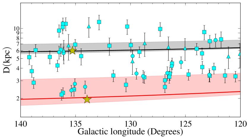
Figure 11: The spatial distribution of our CBe stars on the Galactic Plane is shown. Different symbols are used for the luminosity class: dwarf (squares), circles (sub-giants), triangles (giants). The spiral arms are plotted following the prescriptions given in Vallée (2008) – solid red curve for the Perseus Arm, black solid curve for the Outer Arm. Instead, the two bands of width 1.4 kpc (Russeil, Adami, & Georgelin, 2007), represent the range of distances that are covered by the two spiral arms in (Russeil, Adami, & Georgelin, 2007). The Perseus Arm is in pink, the Outer Arm is in grey. The two yellow stars mark the trigonometric parallaxes of masers as specified by Reid et al. (2009), which are sitting on the near edge of the spiral arms where the star formation is active.

As a partial test of this method of estimation, we have applied it to photometric selections of A/F stars in the well-studied clusters, NGC 637 and NGC 663. In the case of NGC 637, Yadav et al. (2008) obtained $2.5\pm 0.2$ kpc from conventional photometric methods – our shorthand method gives 2.0 kpc. For NGC 663, we obtain A/F distances for three different sightlines crossing the cluster (to CBe stars for which we have only FLWO-1.5m/FAST spectra) that are respectively 2.2, 2.5, and 2.8 kpc. These compare satisfactorily with the literature measure of $2.4\pm 0.1$ kpc (Pandey et al., 2005) for this cluster. Nevertheless the method carries two potential biases towards low estimates that results in 16 A/F star distances that are much lower than the class V CBe-star distance. First, it rests on trying to identify associated main-sequence A/F stars – although we attempt to eliminate interloping giants (improbable companions for CBe stars), this may not always be successful. Second, where the CBe star is relatively early-type (B2-4) and very distant, the reddening may be comparable with the total Galactic reddening with the result that the detected A/F stars may actually be foreground and unassociated. The first of these biases may result in inappropriate assignment to class V, but the second most likely ’fails safe’ (in 9 of the 16 cases) in leaving these objects as dwarfs at distances of between 8 and 12 kpc. Given these issues, we do not regard these estimates as providing more than an ad hoc sorting tool.

The pattern emerging from the luminosity class assignments is similar to that among the sample of classical Be stars presented by Zorec & Briot (1997): 42 are assigned to class V (cf 36, on scaling to this older result), while 12 and 9 are placed into classes IV and III respectively (cf expectations of 14–15, and 13). That there are more dwarfs may either be a consequence of the much fainter apparent magnitude range our sample is drawn from, or due to the noted bias in the method of assignment.

4.3 Spatial distribution of the CBe sample

In Fig. 11 we plot all the stars at the distance corresponding to their assigned luminosity class against Galactic longitude, marking on the diagram the expected locations of the Perseus and Outer Arms. The four stars for which we do not have spectroscopic ${\rm H}\alpha$ observations are not included in this plot. The emergent picture presented by these 63 stars is certainly not one of pronounced clustering picking out the spiral arms in the distance-longitude plot. Closest to this possible reality is seen at longitude $\sim$135 where there is a group of six stars near the star-forming complexes W3/W4/W5, well in front of another group of stars, sitting closer to the OH maser in the Outer Arm. Elsewhere there is no sign of such orderly behaviour. The casual impression is of a scattered, more or less random, distribution of emission line stars.

In the sample, no CBe star is closer than $2.2\pm 0.3$ kpc (# 56) or more distant than $11.6\pm 2.0$ kpc (# 39). This is mainly a reflection of the magnitude limits ($13\lesssim r\lesssim 16$) placed on the sample of CBe stars. At the bright end $(r=13)$, a main sequence dwarf with a median spectral type (B5), with a median reddening of $A_{r}=2.5$, just falls within the sample at the minimum distance of $\sim 2.0$ kpc. For B3V this estimate of the minimum rises to 2.9 kpc, consistent with the brightest object (# 45) in the sample, that happens to be a B3 star, being assigned a distance of 2.8 kpc (its reddening is a little above the median value). For the latest spectral types present in the sample, the near distance limit drops as low as 1 to 1.5 kpc. That we do not find any in the allowed range between 1 and 2 kpc is perhaps because the reddening only rises up to and through the median for the distribution once the Perseus Arm is well and truly entered at $\sim$2 kpc.

The upper distance limit can in principle be expected to be more variable, following to an extent the variation of the integrated Galactic reddening with sightline ( SFD98, ): for most of the CBe sample the maximum possible $A_{r}$ varies from $\sim$2 up to $\sim$5. But our selection has, for practical observational reasons, avoided the most heavily reddened objects and sightlines (the maximum $A_{r}$ in the sample is 4). On deploying the median spectral type and reddening for the sample, again – but this time combining them with the absolute magnitude appropriate to luminosity class III — we would expect a faint magnitude limit of $r\sim 16$ to translate to a maximum heliocentric distance of $\sim$16 kpc (dropping to 10–12 kpc for the latest B sub-types). The actual outcome is that the most distant/faintest objects in the sample are B3-4Ve objects inferred to be 10–12 kpc away. The objects assigned to luminosity class III are, in contrast, mostly relatively bright and/or relatively heavily reddened, bringing all but one of them in to distances closer than 10 kpc. So whilst there is not a simple upper limiting distance to the observed window, there is reason to assume that the range from 3 to 8 kpc is well captured by our sample at all sub-types – so if CBe stars are preferentially located in the Outer Arm at 5 to 6 kpc, it would be likely to be evident. Fig. 11 does not support this. We return to this below in the discussion.

The most distant early-type dwarf stars at heliocentric distances of 10–11 kpc are 16–17 kpc away from the Galactic Centre. This places them significantly outside the disc ’truncation’ radius estimated by Ruphy et al. (1996), and since re-examined by Sale et al. (2010). Although dependent in detail on how the stellar density profile steepens at these large Galactocentric radii, we would not expect a selection of CBe stars fainter than $r=16$ to yield too many more-distant objects – instead, it would more likely add in stars that are later in spectral type, more reddened, or both. Indeed the number of early-type stars that are already known at such a large Galactocentric radii is very small. In Rolleston et al. (2000), just 14 out of the 80 studied B-type stars, between $6\leq R_{G}\leq 18$ kpc, are found at distances larger than $R_{G}\sim 13$ kpc.

5 Discussion

In this section, we identify the main insights provided by our sample of 67 CBe stars, identifying robust outcomes and possible biases. Regarding the latter, we analyse the impact that choices of reddening law and absolute magnitude scale, and the method of correction for circumstellar disc fraction, may have had on the distance estimates. Finally, we compare (i) the inferred cumulative distribution of object distances with that expected of a regularly declining disc stellar density profile, (ii) the measured corrected colour excesses, $E(B-V)_{\rm{S,\,c}}$, with the integrated colour excesses from SFD98.

5.1 Possible biases

We now turn to the individual biases that may affect the distances inferred for our sample.

5.1.1 The absolute magnitude scale and luminosity classification

In Section 4.1, we pointed out that our chosen absolute magnitude scale is the faintest among those to be found in current literature. For example the MS magnitudes we have adopted are, on average, 0.4-0.6 mag fainter than others reported in literature (see e.g. Straizys & Kuriliene, 1981; Aller et al., 1982; Wegner, 2000) for the early and late-B types, whilst they are better aligned for mid-B stars. Had we favoured a brighter absolute magnitude scale, we should expect to obtain distances up to 25 % larger than those we have tabulated. However it is worth noting that we found that the great majority of our class V spectroscopic parallaxes gave larger values than those crudely inferred from nearby candidate A/F stars (section 4.2 and Table 6). This may turn out to be part of the explanation for the attribution of a somewhat higher proportion of the sample to class V, based on the existing absolute magnitude scale, relative to the earlier sample of Zorec & Briot (1997).

The deduced distance to each CBe star is necessarily strongly dependent on adopted luminosity class. Here, a rough constraint on luminosity class has come from estimating the distances to probable main-sequence A and F stars of comparable reddening within a few arcminutes angular separation (section 4.2). Where the luminosity assignment is wrong by one class, the distance will be over or under-estimated by 30 % – a large uncertainty. To do better, a robust spectroscopic indicator is needed. One possibility under investigation presently is to adapt the Barbier-Chalonge-Divan (BCD) method that evaluates the properties of the Balmer limit (Fabregat et al, in preparation) to the circumstances of the entire FLWO-1.5m/FAST dataset. This will incorporate the subset of stars that we have described here in detail. For the time being it is reassuring that the spread of this smaller sample across luminosity class is not radically different from that found by Zorec & Briot (1997).

At the present time, the uncertainty in absolute magnitude is the major contribution to the error budget for the distance determinations. The errors are large enough that attention must be paid to an error-sensitive statistical bias that was discussed in Feast (1972). This is dependent on the gradient in space density and its impact is quantified in Section 5.2 where we discuss the spatial distribution of the sample.

5.1.2 Disc fraction estimates

We based our disc fraction and circumstellar excess estimates using the commonly adopted method proposed by Dachs, Kiehling, & Engels (1988), in which the measured $E(B-V)_{\rm{S}}$ is corrected downwards using a scaling to the ${\rm H}\alpha$ emission equivalent width. As we already noticed in Sec.3.3, we observed 5 stars with $EW({\rm H}\alpha)\leq-60$ Å, that lie outside the range in which Eq.4 and 5 were defined. This makes their $E^{cs}(B-V)$ determination more uncertain. Furthermore, both of (Dachs, Kiehling, & Engels, 1988) equations are based on quite scattered data.

For the most extreme emitter in our sample (# 26, with $EW({\rm H}\alpha)\approx-100$ Å), a variation of $f_{D}$ twice as large as the 0.02 uncertainty that we considered in the error propagation would move the star by $\pm 5$% around its measured distance, after taking into account the corresponding $E^{cs}(B-V)$ and $\Delta r$ changes. The estimate of $E^{cs}(B-V)$ also has an effect on the identification of the preferred luminosity class, in that a different $E(B-V)_{\rm{(S,\,c)}}$ value alters the selection of stars in the colour-colour diagrams of Sec.4.2 and, hence, the A/F star fits. In short, the role of the disc fraction and the uncertainties in its estimation is complex. It is fortunate that for most of the sample its impact is not likely to be very large

5.1.3 Choice of reddening law

As we mentioned in Section 3.2 a different choice of $R_{V}$ would affect the distance estimates, although the measured colour excesses would not change too much since the shape of the curve does not change significantly if $R_{V}$ is altered by a few tenths. A smaller/larger $R_{V}$ produces lower/higher reddening for a given colour excess, and hence a larger/smaller inferred spectroscopic parallax. A study of the shape of reddening laws across much of the Galactic Plane was undertaken by Fitzpatrick & Massa (2007). Taken at face value, this work would seem to imply a lower $R_{V}$ of $2.9\pm 0.2$ within the region delimited by $\ell=(120^{\circ},140^{\circ})$ and $b=(-5^{\circ},+5^{\circ})$. However this is based only on three bright B stars, that apparently lie on the near side of the Perseus Arm. Since the majority of our stars are appreciably more distant than 2 kpc, there is no strong incentive yet to stray from the widely accepted mean law ($R_{V}=3.1$). Had we preferred $R_{V}=2.9$, the derived spectroscopic parallaxes would be about $8-10\%$ larger than specified here. Conversely, raising $R_{V}$ above the typical Galactic value would shorten the distance scale. If a change in either sense is necessary, it is more likely that $R_{V}$ should be increased.

5.2 The cumulative distribution of CBe-star distances

In this part of the Galactic Plane ($120^{\circ}\leq\ell\leq 140^{\circ}$ and $-1^{\circ}\leq b\leq 4^{\circ}$), Galactic models (Russeil, 2003; Vallée, 2008) place the Perseus Arm at $\sim 2$ kpc and the Outer Arm at $\sim 6$ kpc, consistent with measured maser parallaxes (Reid et al., 2009). We showed in Fig. 11 the distances to 63 of the 67 objects presented in this paper as a function of Galactic longitude, leaving out 4 objects for which we do not have the H$\alpha$ emission equivalent width data needed to correct the measured reddenings for circumstellar emission, and one further star that is more likely to be a YSO. Neither this figure, nor the binned histogram distribution shown in Fig. 12, displays a pronounced clustering consistent with these mooted spiral arm locations.

We reconsider the distribution collapsed into a cumulative form that permits an analysis free of binning effects (Fig. 12). The magenta curve shown in it is the cumulative distribution as a function of distance obtained when all CBe stars are classified as dwarfs, while the blue curve is the result obtained on assigning luminosity classes as given in Table 6. If the CBe stars were preferentially located in the Perseus and Outer Arms, we might expect to see steepenings of the cumulative distribution curve (CDC) in the distance ranges associated with the Arms (picked out in the figure).

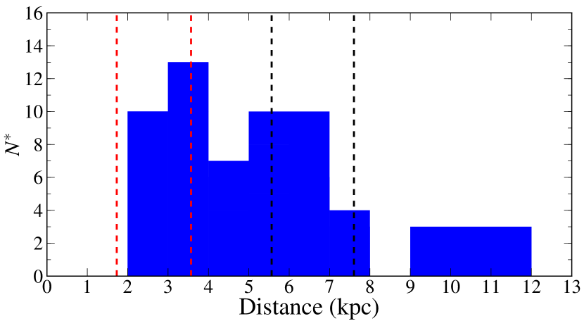
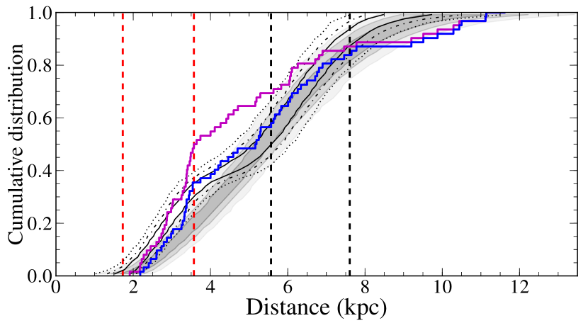
Figure 12: (a) Histogram distribution of stars with luminosity class being assigned accordingly to Table 6. The vertical dashed lines define the distance ranges thought to be occupied by the spiral arms: red is used for the Perseus Arm, black for the Outer Arm. (b) The cumulative distribution of CBe stars is plotted against the distances derived from spectroscopic parallax. The blue curve expresses the distribution of stars that takes note of the preferred luminosity class assignment in Table 6. The dark magenta curve is the result obtained if all the CBe stars are assumed to be class V. The grey-scale contours represent the 1$\sigma$, 2$\sigma$, and 3$\sigma$ confidence limits that result from the MC simulations of a smooth distribution of stars. Similarly, the black curves are for the boundaries defined by the family of CDCs, which are derived from the MC simulations of stars within the spiral arms. Vertical dashed lines define the range of distances associated to the spiral arms, as in panel (a).

To test this expectation, we compare our result with simulated, appropriately randomised CDCs computed using two contrasting models: (i) a stellar density gradient consistent with the average properties of the outer Galactic disc; (ii) a simple spiral arm model in which it is assumed the CBe stars are contained within them. To obtain such CDCs, in the first case we set up a distribution function to be obeyed by the 63 stars that deploys the length scales and disc ’truncation radius’ derived by Sale et al. (2010): essentially the exponential length scale out to $R_{G}=13\pm 0.5$ kpc is $(3.0\pm 0.12)$ kpc, and thereafter it shortens to $(1.2\pm 0.3)$ kpc. In the second case, we distribute the stars along the line-of-sight according to two boxcar functions, whose limits are defined by the allowed range of distances for the Perseus and Outer Arms given in Russeil, Adami, & Georgelin (2007) – the relative weight of the two spiral arms is set to match the exponential decay of case (i). Both distributions are weighted with a $D^{2}$ term, to reproduce the conical volume sample function. To emulate the effect of error in the real data, the randomly selected distances of stars in each simulation are scattered according to gaussian noise, that is modelled as a linear function of distance, fit to the real errors. 10000 Monte Carlo (MC) simulations were performed for each type of model. The starting distance of the two models, set to roughly match the observational selection, does influence the outcome. But we find that placing it anywhere between 1 and 2 kpc does not affect the median CDC produced by the MC simulations. Because of the steep decline in stellar density outside the truncation radius, the end point is not influential.

We plot both comparison CDCs in Fig. 12, in the form of contours defining the 1$\sigma$, 2$\sigma$, and 3$\sigma$ confidence limits derived from the two families of MC simulations. A direct visual comparison between the CDC of the 63 CBe stars (blue curve) and the contours generated with the simulations, indicates that the observations incorporating luminosity class constraints (blue curve) do not clearly prefer either model yet. However, the CDC obtained with all the stars classified as dwarfs (magenta curve) is exposed as implausible, since too many stars are assigned to the Perseus Arm. This is on top of the improbability that all objects in the CBe sample would be dwarfs, given the known properties of these stars.

We have performed K-S tests comparing the observed cumulative functions with the median of the simulated data, from both models. For the magenta curve (all stars being dwarfs), we obtain $D_{\rm{no-arms}}=0.3$ and $p_{\rm{no-arms}}\sim 0$, $D_{\rm{arms}}=0.21$ and $p_{\rm{arms}}=0.12$; due to the large D values and the small p-values, we can reject the hypothesis that the magenta distribution is consistent with either models. On the other hand, for the blue curve we measure $D_{\rm{no-arms}}=0.16$ and $p_{\rm{no-arms}}=0.37$, $D_{\rm{arms}}=0.14$ and $p_{\rm{arms}}=0.51$. In this case the numerical outcome is inconclusive, rather than negative – our CBe sample may be compatible with either model, and it is clear that reduced errors, combined perhaps with a larger sample would be needed for a more decisive outcome.

Furthermore, the astrophysical point that $\sim 60$% of the stars in our sample are B5 or later in spectral type should not be overlooked: if the Be phenomenon is due to evolutionary structural changes (Fabregat & Torrejón, 2000), these later-type stars would be less likely to have remained within the spiral arms at an age approaching 50 Myr or more, than their earlier-type cousins. Ideally, a larger sample restricted to early-type Be stars, if feasible, would supply the best test for the spiral arm structure of the Galaxy.

We note that the statistical bias of the type first set out by Feast (1972) and implemented by Balona & Feast (1974) is present here. Since the error model adopted for the MC simulations is based on the uncertainties affecting the real data, the impact of the bias can be gauged numerically just by comparing the error-free model CDC with its form when the error is included. We find, in accordance with expectation, that the shorter distances in the sample are under-estimated, and the longest are over-estimated. The effect is most severe at the longest distances ($>8$ kpc) where the over-estimation may approach 1 kpc. At $\sim 2$ kpc, the under-estimation is in the region of 100-200 pc. Since our MC simulation already takes into account this bias, the outcome of the K-S test reported above also accounts for it.

Before now, by means of OB-star spectroscopic parallaxes derived from a brighter sample ($8<V<13$) of stars than here, Negueruela & Marco (2003) identified a number of OB stars at $d\approx 5.3$ kpc for $115^{\circ}<\ell<120^{\circ}$ and $d=5$ – 6 kpc for $\ell=175^{\circ}$ – $215^{\circ}$. Thanks to the high quality of their spectroscopic data, the authors felt able to claim spectral types had been determined to a precision better than $\pm 1$ subtype, yielding distances with errors less than 10%. They surmised that these objects could belong to the Outer Arm, but stopped short of claiming detection of a spiral arm, as such. Within the same Galactic longitude range as considered here, they had very few stars at their disposal. Here we have filled in this gap – but still we do not claim that either Fig. 11 or the preferred blue curve in Fig. 12, accounting for the range of luminosity classes present in the sample, rules in or out an Outer Arm at 5–6 kpc.

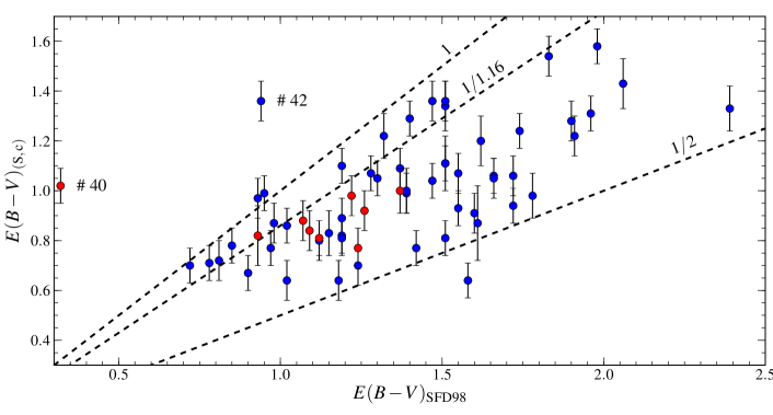
Figure 13: The corrected colour excesses for the CBe star sample is plotted against the corresponding integrated Galactic colour excesses from SFD98, for each sightline. Red symbols are used for the stars with a measured distance larger than 8 kpc, well beyond the expected location of the Outer Arm. The three dashed black lines are linear relations of the form $E(B-V)_{\rm{(S,\,c)}}=mE(B-V)_{\rm{SFD98}}$, where $m=1,\,1/1.16,\,1/2$ respectively.

5.3 Comparison with total Galactic colour excesses from SFD98

CBe stars are massive, intrinsically-luminous stars capable of being seen to very large distances. Among the current sample, there are several examples of CBe stars at distances large enough to indicate they lie beyond even the putative Outer Arm. The reddening of such objects ought to closely match the integrated Galactic value since little Galactic dust should lie beyond them in the far outer disc. Less distant CBe stars should in general exhibit reddenings below the total for the relevant sightline.

The most widely used source of integrated reddenings is the work of SFD98. We have plotted the measured colour-excess, $E(B-V)_{\rm{(S,\,c)}}$, for each CBe star against the colour excess, $E(B-V)_{\rm{SFD98}}$, provided by SFD98 (Fig. 13: both values are listed in Table 3). The former is a spot value pertaining to a single line of sight, while the latter applies to a spatial resolution element about 6 arcmins across. Hence it should be kept in mind that small variations in the ISM will add a random noise element to the comparisons we make. We continue to exclude the four stars that do not have a measured $EW({\rm H}\alpha)$ in Table 3. A general property of the diagram is that for all but two objects, $E(B-V)_{\rm{SFD98}}>E(B-V)_{\rm{(S,\,c)}}$, to within the errors. This accords with expectation.

The stars shown in red are the most distant, at more than 8 kpc away, whose reddenings should most nearly match the total Galactic value (these are specifically, objects # 11, 26, 35, 39, 40, 50, 54, 55, and 60). All but one of these stars (# 40) are early-B dwarfs. However, apart from # 40, we find that the measured colour excesses for these objects are distinctly less than those from the SFD98 reddening map. The discrepancy is of order 0.2-0.3 magnitudes. This undershoot is broadly in keeping with the result of Chen et al. (1999) that SFD98 typically overestimate the reddening by a factor of 1.16. To illustrate this, a second reference line is drawn in figure 13 with this correction applied.

For object # 40 the situation is quite different, since the datum from SFD98 indicates a very much lower total dust column than we obtain. We notice in the SFD98 temperature map (that is much less well-resolved spatially than the emissivity map) a large hot spot roughly corresponding to the upper part of the galactic chimney linked to W4 (cf. Normandeau, 2000; Terebey et al., 2003): it seems plausible therefore that the cause of the problem is the adoption of too high a dust temperature for this particular sightline predicting too low a dust column. A similar but not so extreme discrepancy arises in the case of object # 42.

A further group of stars can be picked out in Fig. 13, whose colour excesses fall above the lower reference line but remain compatible with or below the SFD98 equality line. They are objects # 17, 19, 22, 32, 41, 44, 49, 51, 52, 61, 64. As their estimated distances either exceed $\sim 6$ kpc, or their sightlines are at latitudes higher than $b=2^{\circ}$ it is conceivable these objects also lie beyond most/all of the dust column. Alternatively if the scaling down of the SFD98 reddening by a factor of 1.16 is consistently the better guide to the total Galactic value, it might be concluded our reddenings for these stars are too high, perhaps through under-correction for the circumstellar disc contribution, and their estimated distances too low.

A clear feature of the sample as a whole is that their measured reddenings are a significant fraction of the sightline total, ranging from about half the SFD98 value up to rough equality with it. These large fractions of the total dust columns are to be expected given the long sightlines to these intrinsically bright objects.

6 Conclusions

In this study, we investigated a 100 deg² portion of the Galactic Plane, between $120^{\circ}\leq\ell\leq 140^{\circ}$ and $-1^{\circ}\leq b\leq 4^{\circ}$, that includes a part of the Perseus Arm, $\sim$2 kpc away and of the less well-established Outer or Cygnus Arm, 5–6 kpc distant.

We studied a group of 67 candidate classical Be stars that we selected among 230 that in turn were selected from follow-up of candidate emission line stars. We determined their spectral types with an estimated accuracy of $\pm 1$ sub-type and measured colour excesses via SED fitting in the blue (3800 – 5000 Å), and made appropriate correction for the contribution to the colour excess for circumstellar emission. Distances were determined via spectroscopic parallaxes, after luminosity classes had been assessed using MS fits to A/F stars of similar reddening selected via colour-cuts from IPHAS photometry, in the vicinity of each CBe star. Our main findings are:

• IPHAS offers very effective, easy selection of moderately reddened ($E(B-V)\sim 1$) classical Be candidates: their identity has been confirmed by a combination of low resolution optical spectroscopy and infrared photometry.

• Our magnitude limited sample ($r\leq 16$) includes 10–15 stars in the outer disc at Galactocentric radii where the stellar density gradient is likely to be steepening ($R_{\rm{G}}\geq 13$ kpc, or heliocentric distances greater than 7 kpc). These objects exhibit reddenings comparable with those obtained from the map of Schlegel, Finkbeiner, & Davis (1998), serving to emphasise how far out in the Galactic disc they are.

• The errors on the distance estimates remain too large to obtain a decisive statistical test of models for the spatial distribution of the CBe stars. The major, presently irreducible, contribution to the error budget is the spread of absolute magnitude associated with a given spectral type.

These first results will be investigated in more depth, using a much larger sample of $\sim 200$ classical Be star candidates observed with FAST, aided by extinction-distance curves built from IPHAS photometry (using a new Bayesian implementation of MEAD, Sale, 2012). This approach has the potential to provide a better grip on both luminosity class and distance even in the absence of precise absorption-line diagnostics. The longer term prospect is that astrometry returned by the Gaia mission, due to launch in 2013, will greatly improve the distances estimated for samples of objects like the one presented in this study. From predicted end-of-mission performance data (de Bruijne, 2012), it appears we can look forward to $5-10$% parallax errors for our objects perhaps within the decade, as compared with up to 20% presently. Especially when accompanied by carefully measured extinctions, that are essential for clarifying intrinsic absolute magnitudes, further enlargement of the sample of well-characterised fainter CBe stars will provide an avenue to better test our knowledge both of Galactic structure and of massive-star evolution.

References

- Aller et al. (1982) Aller L. H., et al., 1982, Landolt-Börnstein: Numerical Data and Functional Relationships in Science and Technology, Vol 2, Springer-Verlag, Berlin
- Balona & Feast (1974) Balona L. A., Feast M. W., 1974, MNRAS, 167, 621
- Bertout (1989) Bertout, C. 1989, ARA&A, 27, 351
- Bessell & Brett (1988) Bessell, M. S. & Brett, J. M. 1988, PASP, 100, 1134
- Cambrésy, Jarrett, & Beichman (2005) Cambrésy L., Jarrett T. H., Beichman C. A., 2005, A&A, 435, 131
- Carciofi & Bjorkman (2006) Carciofi, A. C. & Bjorkman, J. E. 2006, ApJ, 639, 1081
- Carpenter (2001) Carpenter, J. M. 2001, AJ, 121, 2851
- Carpenter, Heyer, & Snell (2000) Carpenter, J. M., Heyer, M. H., & Snell, R. L. 2000, ApJS, 130, 381
- Chauville et al. (2001) Chauville, J., Zorec, J., Ballereau, D., Morrell, N., Cidale, L., & Garcia, A. 2001, A&A, 378, 861
- Chen et al. (1999) Chen B., Figueras F., Torra J., Jordi C., Luri X., Galadí-Enríquez D., 1999, A&A, 352, 459
- Corradi et al. (2008) Corradi R. L. M., et al., 2008, A&A, 480, 409
- Cutri et al. (2003) Cutri R. M., et al., 2003, tmc..book,
- Dachs, Kiehling, & Engels (1988) Dachs J., Kiehling R., Engels D., 1988, A&A, 194, 167
- Dachs, Rohe, & Loose (1990) Dachs J., Rohe D., Loose A. S., 1990, A&A, 238, 227
- Dame, Hartmann, & Thaddeus (2001) Dame T. M., Hartmann D., Thaddeus P., 2001, ApJ, 547, 792
- de Bruijne (2012) de Bruijne J. H. J., 2012, Ap&SS, 341, 31
- Didelon (1982) Didelon P., 1982, A&AS, 50, 199
- Drew (1989) Drew, J. E. 1989, ApJS, 71, 267
- Drew et al. (2005) Drew J. E., et al., 2005, MNRAS, 362, 753
- Drew et al. (2008) Drew J. E., Greimel R., Irwin M. J., Sale S. E., 2008, MNRAS, 386, 1761
- Fabregat & Torrejón (2000) Fabregat J., Torrejón J. M., 2000, A&A, 357, 451
- Fabricant et al. (1998) Fabricant D., Cheimets P., Caldwell N., Geary J., 1998, PASP, 110, 79
- Feast (1972) Feast M. W. 1972, Vistas in Astronomy, 13, 207
- Fitzpatrick (1999) Fitzpatrick E. L., 1999, PASP, 111, 63
- Fitzpatrick & Massa (2007) Fitzpatrick E. L., Massa D., 2007, ApJ, 663, 320
- Freudenreich et al. (1994) Freudenreich H. T., et al., 1994, ApJ, 429, L69
- Gray & Corbally (2009) Gray R. O., Corbally C., J., 2009, Stellar Spectral Classification, Princeton University Press
- Hachisuka et al. (2009) Hachisuka K., Brunthaler A., Menten K. M., Reid M. J., Hagiwara Y., Mochizuki N., 2009, ApJ, 696, 1981
- Houk et al. (1997) Houk N., Swift C. M., Murray C. A., Penston M. J., Binney J. J., 1997, ESASP, 402, 279
- Humphreys (1976) Humphreys R. M., 1976, PASP, 88, 647
- Jaschek & Jaschek (1987) Jaschek C., Jaschek M., 1987, The classification of stars, Cambridge: University Press
- Jones, Tycner, & Smith (2011) Jones C. E., Tycner C., Smith A. D., 2011, AJ, 141, 150
- Kaiser (1989) Kaiser D., 1989, A&A, 222, 187
- Kenyon & Hartmann (1995) Kenyon S. J., Hartmann L., 1995, ApJS, 101, 117
- Lada & Adams (1992) Lada C. J., Adams F. C., 1992, ApJ, 393, 278
- Levine, Blitz, & Heiles (2006) Levine E. S., Blitz L., Heiles C., 2006, Sci, 312, 1773
- Megeath et al. (2008) Megeath S. T., Townsley L. K., Oey M. S., Tieftrunk A. R., 2008, Handbook of Star Forming Regions, Volume I: The Northern Sky ASP Monograph Publications, Vol. 4. Edited by Bo Reipurth, p.264
- Meyer, Calvet, & Hillenbrand (1997) Meyer M. R., Calvet N., Hillenbrand L. A., 1997, AJ, 114, 288
- Munari et al. (2005) Munari U., Sordo R., Castelli F., Zwitter T., 2005, A&A, 442, 1127
- Negueruela & Marco (2003) Negueruela I., Marco A., 2003, A&A, 406, 119
- Normandeau (2000) Normandeau, M. 2000, Stars, Gas and Dust in Galaxies: Exploring the Links, 221, 41
- Pandey et al. (2005) Pandey A. K., Upadhyay K., Ogura K., Sagar R., Mohan V., Mito H., Bhatt H. C., Bhatt B. C., 2005, MNRAS, 358, 1290
- Porter & Rivinius (2003) Porter J. M., Rivinius T., 2003, PASP, 115, 1153
- Reid et al. (2009) Reid M. J., et al., 2009, ApJ, 700, 137
- Rieke & Lebofsky (1985) Rieke G. H., Lebofsky M. J., 1985, ApJ, 288, 618
- Rolleston et al. (2000) Rolleston W. R. J., Smartt S. J., Dufton P. L., Ryans R. S. I., 2000, A&A, 363, 537
- Ruphy et al. (1996) Ruphy S., Robin A. C., Epchtein N., Copet E., Bertin E., Fouque P., Guglielmo F., 1996, A&A, 313, L21
- Russeil (2003) Russeil D., 2003, A&A, 397, 133
- Russeil, Adami, & Georgelin (2007) Russeil D., Adami C., Georgelin Y. M., 2007, A&A, 470, 161
- Sale et al. (2009) Sale S. E., et al., 2009, MNRAS, 392, 497
- Sale et al. (2010) Sale S. E., et al., 2010, MNRAS, 402, 713
- Sale (2012) Sale, S. E. 2012, arXiv:1208.4946
- Schlegel, Finkbeiner, & Davis (1998) Schlegel D. J., Finkbeiner D. P., Davis M., 1998, ApJ, 500, 525
- Siess, Forestini, & Dougados (1997) Siess L., Forestini M., Dougados C., 1997, A&A, 324, 556
- Steiman-Cameron, Wolfire, & Hollenbach (2010) Steiman-Cameron T. Y., Wolfire M., Hollenbach D., 2010, ApJ, 722, 1460
- Straizys & Kuriliene (1981) Straizys V., Kuriliene G., 1981, Ap&SS, 80, 353
- Terebey et al. (2003) Terebey, S., Fich, M., Taylor, R., Cao, Y., & Hancock, T. 2003, ApJ, 590, 906
- Valdes et al. (2004) Valdes F., Gupta R., Rose J. A., Singh H. P., Bell D. J., 2004, ApJS, 152, 251
- Vallée (2008) Vallée J. P., 2008, AJ, 135, 1301
- Vázquez et al. (2008) Vázquez R. A., May J., Carraro G., Bronfman L., Moitinho A., Baume G., 2008, ApJ, 672, 930
- Waters & Waelkens (1998) Waters L. B. F. M., Waelkens C., 1998, ARA&A, 36, 233
- Wegner (2000) Wegner, W. 2000, MNRAS, 319, 771
- Witham et al. (2008) Witham A. R., Knigge C., Drew J. E., Greimel R., Steeghs D., Gänsicke B. T., Groot P. J., Mampaso A., 2008, MNRAS, 384, 1277
- Xu et al. (2006) Xu Y., Reid M. J., Zheng X. W., Menten K. M., 2006, Sci, 311, 54
- Yadav et al. (2008) Yadav R. K. S., Kumar B., Subramaniam A., Sagar R., Mathew B., 2008, MNRAS, 390, 985
- Zorec & Briot (1991) Zorec J., Briot D., 1991, A&A, 245, 150
- Zorec & Briot (1997) Zorec J., Briot D., 1997, A&A, 318, 443