Non-abelian gauge fields and quadratic band touchings in molecular graphene

Abstract

Dirac fermions in graphene can be subjected to non-abelian gauge fields by implementing certain modulations of the carbon site potentials. Artificial graphene, engineered with a lattice of CO molecules on top of the surface of Cu, offers an ideal arena to study their effects. In this work, we show by symmetry arguments how the underlying CO lattice must be deformed to obtain these gauge fields, and estimate their strength. We also discuss the fundamental differences between abelian and non-abelian gauge fields from the Dirac electrons point of view, and show how a constant (non-abelian) magnetic field gives rise to either a Landau level spectrum or a quadratic band touching, depending on the gauge field that realizes it (a known feature of non-abelian gauge fields known as the Wu-Yang ambiguity). We finally present the characteristic signatures of these effects in the site-resolved density of states that can be directly measured in the current molecular graphene experiment, and discuss prospects to realize the interaction induced broken symmetry states of a quadratic touching in this system.

I Introduction

Condensed matter systems that host Dirac fermions as their electronic excitations have drawn a lot of attention in recent years as they have become more and more experimentally accesible and controlable, with grapheneCGP09 and topological insulatorsHK10 being the most prominent examples of such materials.

A remarkable feature of Dirac fermions realized in graphene’s honeycomb lattice in particular is that one can further manipulate them externally by inducing controlled strains in the sample, which couple to them as an effective gauge potentialVKG10 . This idea of strain engineeringPC09 has led to many interesting predictionsGKG10 ; JCV11 , and is most spectacularly illustrated by the Landau level spectrum recently observedLBM10 in scanning tunneling microscopy (STM). This system proved to be very versatile, and in search for even better tunability several proposals were conceived to make artificial versions of itPL09 ; GSP09 ; SGK11 . In a recent experimental breakthrough, a realization of this type of systems, termed molecular grapheneGMK12 , was built, which allows for almost complete control of the electronic degrees of freedom within it. In this system, a triangular lattice of CO molecules is assembled in the surface of bulk Cu, confining the surface electrons to move in an effective hexagonal potential. In this way, effective Dirac fermions emerge at the $K$ points of the superlattice potential, which can then be probed directly with an STM.

This system thus offers wide tunability to modify the electronic structure of the surface states by distorting the CO lattice in any desired way, or by adding new atoms to the existing structure. Indeed, several remarkable phenomena have already been demonstratedGMK12 beyond the strain induced Landau levels, such as the opening of a gap by means of a Kekulé distortion or the creation of an n-p-n junction. Other interesting proposals such as the observation of fractional charge in a vortex HCM07 ; B12 or the synthesis of a quantum spin Hall phaseGGH12 should also be experimentally accesible.

As noted in ref. GGR12, , artificial graphene should be also ideal to explore the more recent prediction that a full $SU(2)$ non-abelian gauge field is in fact realizable in this system, and the strain induced one is just one component of it. Non-abelian gauge fields (of singular nature) were known to emerge in graphene due to disclinations in the latticeGGV93 , but they can also be generated in a smooth fashion by modulating the on-site potential of the carbon atoms in a certain way. As we will discuss, the effects of non-abelian gauge fields can be very different from their abelian counterparts, and it is the purpose of this work to discuss how to adapt the molecular graphene experiment to probe these differences. In particular, we will show that a quadratic band touching can be generated with these fields, allowing a controlled simulation of this band structure which is prone to many-body instabilitiesWAF10 ; MEM11 ; VJB12 .

In general, effective external gauge fields acting on a fermion system may have non-abelian structure when the fermions have internal degrees of freedom, and the gauge field is a matrix acting on this degree of freedom $\vec{A}_{ab}$ whose components need not commute. A typical condensed matter example is spin and the spin-orbit interaction, which can be modeled as an SU(2) gauge field FS93 ; T08 , but there are many more examples WZ84 ; OBS05 ; RJO05 ; DGJ11 . A more recent one is bilayer graphene SGG12 , where the two components of the SU(2) doublet correspond to the wave functions in the two layers, and the interlayer interaction plays the role of the gauge field. In the case of monolayer graphene, the SU(2) doublet is made with the valley degree of freedom GGR12 .

The non-abelian field strength is defined in terms of the covariant derivative $D_{i}=\partial_{i}-iA_{i}$ as $F_{ij}=[D_{i},D_{j}]=\partial_{i}A_{j}-\partial_{j}A_{i}-i[A_{i},A_{j}]$, which in two dimensions gives rise to a non-abelian magnetic field of the form

$$B^{\alpha}=\vec{\partial}\times\vec{A}^{\alpha}+\epsilon^{\alpha\beta\gamma}\vec{A}^{\beta}\times\vec{A}^{\gamma},$$ (1)

where $\vec{A}_{ab}=\vec{A}^{\alpha}\Lambda^{\alpha}_{ab}$ with $\Lambda^{\alpha}_{ab}$ the generators of SU(2), repeated indices are summed, and $\alpha=x,y,z$ (the indices $ab$ will be implicit from now on). The last term in this expression arises because of the non-commutativity of the field components and makes non-abelian gauge fields fundamentally different from their abelian counterparts. In particular, it is responsible for a tricky feature of these gauge fields known as the Wu-Yang ambiguity WY75 : the fact that one may have physically distinct gauge fields (i.e. not gauge equivalent) with the same magnetic field. Indeed, consider these two simple examplesFSW97 . The first (type I) is $\vec{A}^{(3)}=B/2(-y,x)$, $\vec{A}^{(1)}=\vec{A}^{(2)}=0$, which we recognize as the analog of the symmetric gauge for constant (abelian) magnetic field $B$, in this case in the $z$ direction. The second (type II) is $\vec{A}^{(1)}=\sqrt{B/2}(1,0)$, $\vec{A}^{(2)}=\sqrt{B/2}(0,1)$ and $\vec{A}^{(3)}=0$, it also gives constant field $B_{0}$ due to the second term in eq. (1), and it is not gauge related to type I. The magnetic field alone is therefore not enough to distinguish these two cases, but we will see that the spectrum obtained for each case is very different, and this is the physics that, as we will show, can be probed directly in the molecular graphene experiment.

	Valley diagonal		Valley off-diagonal
Rep.	Symm. adapted	$\sigma_{i}\otimes\tau_{j}$	Symm. adapted	$\sigma_{i}\otimes\tau_{j}$
$A_{1}$	$\mathcal{I}$	$\mathcal{I}$	$\Lambda_{x}\Sigma_{z}$	$\sigma_{x}\tau_{x}$
$B_{1}$	$\Lambda_{z}$	$\tau_{z}$	$\Lambda_{y}\Sigma_{z}$	$\sigma_{x}\tau_{y}$
$A_{2}$	$\Sigma_{z}$	$\sigma_{z}\tau_{z}$	$\Lambda_{x}$	$-\sigma_{y}\tau_{y}$
$B_{2}$	$\Sigma_{z}\Lambda_{z}$	$\sigma_{z}$	$\Lambda_{y}$	$\sigma_{y}\tau_{x}$
$E_{1x}$	$\Sigma_{x}$	$\sigma_{x}\tau_{z}$	$\Lambda_{x}\Sigma_{y}$	$-\tau_{y}$
$E_{1y}$	$\Sigma_{y}$	$\sigma_{y}$	$-\Lambda_{x}\Sigma_{x}$	$\sigma_{z}\tau_{x}$
$E_{2x}$	$-\Lambda_{z}\Sigma_{y}$	$-\sigma_{y}\tau_{z}$	$\Lambda_{y}\Sigma_{x}$	$-\sigma_{z}\tau_{y}$
$E_{2y}$	$\Lambda_{z}\Sigma_{x}$	$\sigma_{x}$	$\Lambda_{y}\Sigma_{y}$	$\tau_{x}$

Table 1: Classification of basis matrices in the low energy theory around the $K$,$K^{\prime}$ points in graphene according to the representations of the symmetry group $C_{6v}$, and their explicit realization in the basis $(\psi_{AK},\psi_{BK},\psi_{AK^{\prime}},\psi_{BK^{\prime}})$ (see ref. B08, for details).

II Symmetry analysis and microscopic calculation

To realize an SU(2) gauge field in graphene, what we need is to externally apply certain on-site potential patternsGGR12 to the carbon atoms of the honeycomb lattice. It is not a priori clear, however, how this may be achieved in a molecular graphene experiment, where the “effective honeycomb lattice“ is engineered with the potential landscape induced by a triangular array of CO molecules. In terms of an effective tight binding model, it is natural to think that small distortions of this triangular lattice will produce potential changes in the effective carbon sites, but what distortions will give rise to the correct potentials? And more importantly, since these distortions may induce changes in the effective hopping as wellGMK12 , is it possible to modulate only the on-site potential?

To answer these questions, a symmetry approach to the problem appears better suited. The way that external perturbations couple to the low energy degrees of freedom around a high-symmetry point of the Brillouin Zone can be determined just by symmetry arguments. This approach has been fruitfully employed in graphene to discuss the coupling of phonons, strains, or electromagnetic fields M07 ; B08 ; WZ10 ; L12 and we now show how it can be used to see the emergence of non-abelian gauge fields from small CO displacements the molecular graphene.

In the half-filled honeycomb lattice, electrons close to the Fermi surface live near the $K$ and $K^{\prime}$ points, and are described by an effective spinor $(\psi_{AK},\psi_{BK},\psi_{AK^{\prime}},\psi_{BK^{\prime}})$, where $A/B$ denotes the sublattice degree of freedom. The effective Hamiltonian is conventionally written in the basis of the Pauli matrices $\sigma_{i}\otimes\tau_{j}$, where $\sigma_{i}$ acts on the sublattice and $\tau_{i}$ on the valley degrees of freedom, and $i=x,y,z$ (the identity in both sets is understood to be included as part of the basis).

To exploit the fact that the Hamiltonian must be a scalar under the symmetry group $C_{6v}$ of the honeycomb lattice, one can relabel these basis matrices in terms of a new symmetry adapted set $\Sigma_{i}$ and $\Lambda_{i}$ with the Pauli matrix algebra and well-defined transformation properties under this group (technically, the group is $C_{6v}^{\prime\prime}$ because the unit cell has been tripled to consider $K$ and $K^{\prime}$ at the same time. We will refer to the labels under $C_{6v}$ for simplicity, see ref. B08, for details). The relation of these matrices to the original ones and the representations according to which they transform are reproduced in table 1.

In this basis, the low energy Hamiltonian is simply written as ($v_{F}=1$)

$$H=\vec{\Sigma}\cdot\vec{k},$$ (2)

and in this form it is simple to see that the matrices $\Lambda_{i}$ commute with the Hamiltonian and generate an SU(2) symmetry, which corresponds to rotations in the valley degree of freedom.

A gauge field is by definition a field that couples minimally in the form $k_{i}\rightarrow k_{i}+A_{i}$, and in analogy with the usual electromagnetic field that couples as $H_{U(1)}=\vec{\Sigma}\cdot\vec{A}$, one may introduce an SU(2) gauge field that couples as

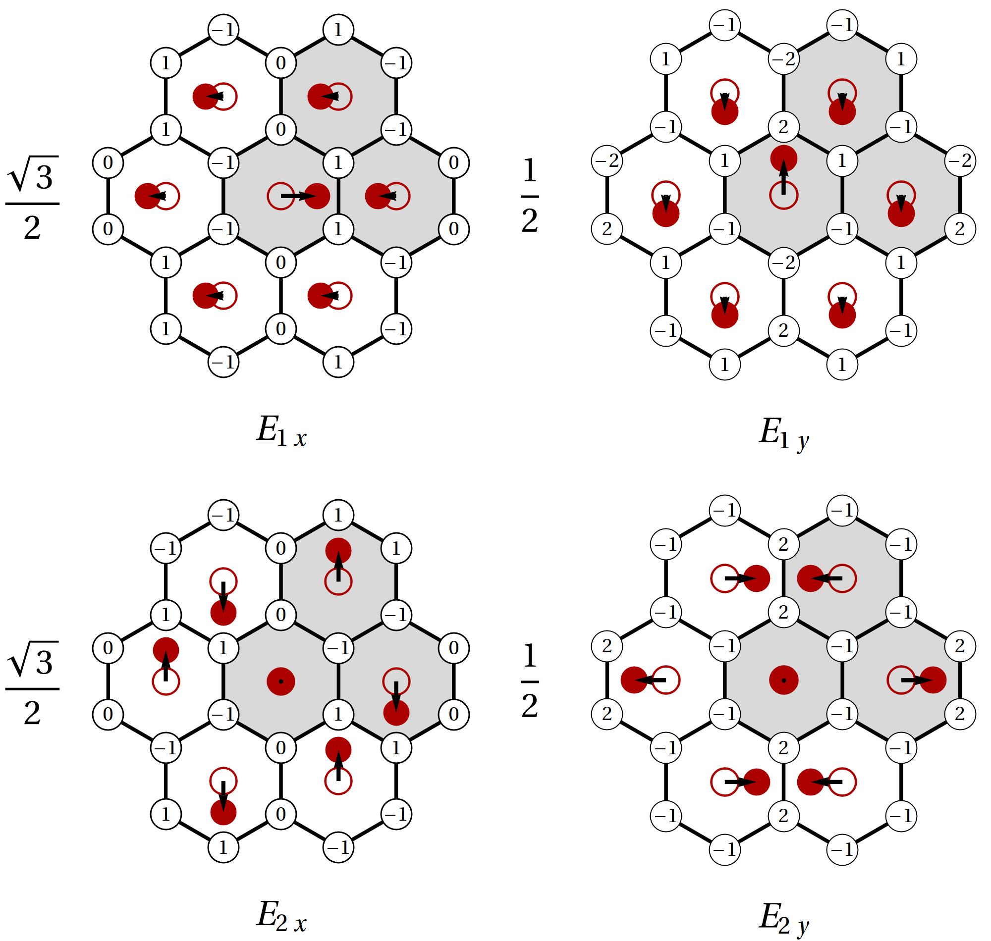
Figure 1: (Color online) The four possible CO displacements with symmetries $E_{1}$ and $E_{2}$. The CO molecules are represented in red, and the effective honeycomb lattice is shown in black. The unit cell is shaded in gray, but more hexagons are shown to make the symmetry of the modes apparent. The on-site potentials that match the symmetry labels are also shown in the effective carbon sites. Note that the prefactors only refer to the potentials, not to the displacements. One may think of these displacements as the K-point phonons of the triangular CO lattice.

$$H_{SU(2)} =\vec{\Sigma}\cdot\left(\Lambda_{x}\vec{A}^{(x)}+\Lambda_{y}\vec{A}^{(y)}+\cdot\Lambda_{z}\vec{A}^{(z)}\right),$$ (3)

which is a coupling allowed by symmetry if the gauge fields $\vec{A}^{\alpha}$ have their origin in a microscopic perturbation with the same symmetry as the matrix that accompanies them.

The power of the symmetry analysis is thus that one can now say what type of perturbations correspond to each term only by inspection of table 1. Perturbations in the first column have the periodicity of the unit cell, while those in the second column have the periodicity of a tripled unit cell (because of intervalley mixing). Moreover, within nearest neighbour tight binding (TB), those perturbations diagonal in sublattice ($\propto\sigma_{0}$ or $\sigma_{z}$) correspond to potential modulations, while those off diagonal correspond to hopping modulations. With this criterion, the gauge field $\vec{A}^{(z)}$ is readily identified as the usual strain-induced gauge field. The gauge field components $\vec{A}^{(x)}$ and $\vec{A}^{(y)}$ correspond, respectively, to the valley mixing $E_{1}$ and $E_{2}$ potential perturbations defined in ref. B08, (which are labeled $G^{\prime}$ under $C_{6v}^{\prime\prime}$). Their corresponding potentials are depicted in fig. 1 in the effective carbon sites.

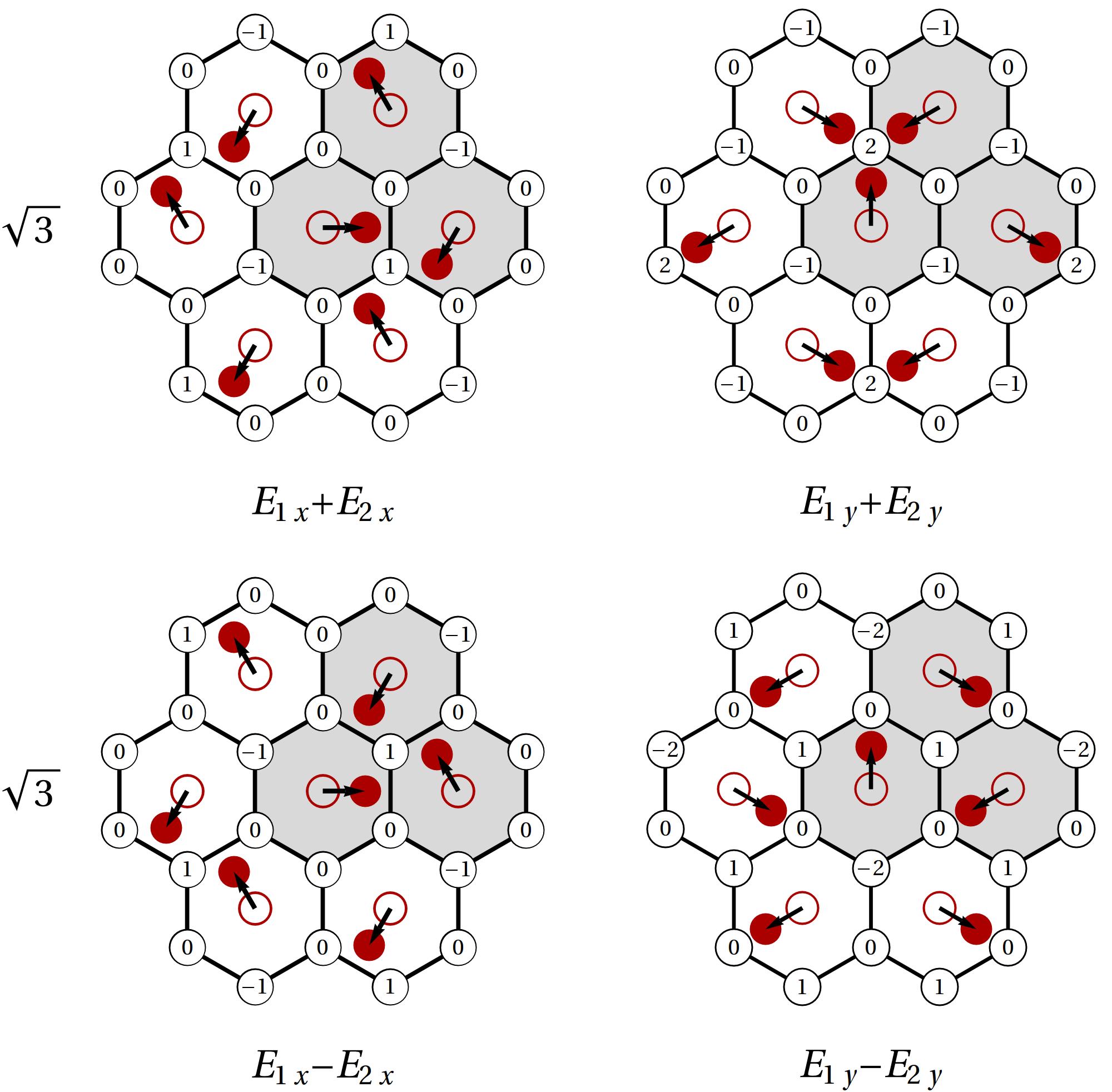
Figure 2: (Color online) With the same conventions that fig. 1, combinations of CO displacements that produce a quadratic band touching. Again, note that the prefactors only refer to the potentials, not to the displacements.

In real graphene this type of potential perturbation is the one induced by phonons like the LO/LA phonon at the K point Falko , or the ZO/ZA phonon at the K point in the presence of a perpendicular electric field, and it is known that it can also be produced by a particular substrate Pankratov .

For molecular graphene, this analysis immediately allows to find the CO displacements that will induce these potential modulations. These should be displacements with a tripled unit cell and the appropriate symmetry labels, and in fact may be simply interpreted as the $E_{1}$ and $E_{2}$ phonons of the triangular CO lattice at the $K$ point. These displacements are, for three consecutive CO molecules

$$\vec{r}_{CO,E_{1x}} =\left\{(1,0)\;,\;(-\tfrac{1}{2},0)\;,\;(-\tfrac{1}{2},0)\right\},$$

$$\vec{r}_{CO,E_{1y}} =\left\{(0,1)\;,\;(0,-\tfrac{1}{2})\;,\;(0,-\tfrac{1}{2})\right\},$$

$$\vec{r}_{CO,E_{2x}} =\left\{(0,0)\;,\;(0,-\tfrac{\sqrt{3}}{2})\;,\;(0,\tfrac{\sqrt{3}}{2})\right\},$$

$$\vec{r}_{CO,E_{2x}} =\left\{(0,0)\;,\;(\tfrac{\sqrt{3}}{2},0)\;,\;(-\tfrac{\sqrt{3}}{2},0)\right\},$$

and are also shown in fig 1. Indeed, within a TB model one can parametrize the change in on-site potential with displacement as

$$V_{i}=V^{\prime}\sum_{j}\Delta\vec{r}_{j,CO}\cdot\vec{\delta}_{ij},$$ (4)

for a carbon site $i$ with $j$ CO neighbours at equilibrium distances $\delta_{ij}$ from it, and verify that the potentials shown in fig. 1 are given by eq. (4). The constant $V^{\prime}\equiv\partial V/\partial a$ parametrizes the change in on-site potential with distance, and may be estimated by realizing that this physical mechanism is responsible for the scalar potential $\phi$ in the continuum Dirac equation. A comparison with the p-n junction experiment yields $V^{\prime}\approx 22$ $\text{meV}/\text{\AA}$ (see appendix), which is very similar to $\partial t/\partial a=\beta t/a\approx 20$ $\text{meV}/\text{\AA}$. This is also consistent with the fact that in real graphene the analog of $V^{\prime}$ for carbon displacementsFalko is of the same order as $\partial t/\partial a$.

Finally, the symmetry analysis also reveals that close to the Dirac point, the desired CO displacements do not introduce any other change in the effective theory other than the $\vec{A}^{(x)},\vec{A}^{(y)}$ gauge fields. In particular, while these displacements may induce nearest neighbour hopping changes, these cannot appear in the low energy theory because there are no intervalley matrices in the $E_{1}$ or $E_{2}$ representations that are sublattice off-diagonal. This hopping changes thus have no effect in the low energy properties and we will not consider them in what follows. Changes in the next nearest neighbour hopping $t^{\prime}$ due this displacements are small and need not be considered.

To obtain the gauge field from a microscopic calculation, one may substitute eq. (4) in the effective tight binding model

$$H=-t\sum_{\left<i,j\right>}c^{\dagger}_{i}c_{j}-t^{\prime}\sum_{\left<\left<i,j\right>\right>}c^{\dagger}_{i}c_{j}+\sum_{i}V_{i}c^{\dagger}_{i}c_{i}.$$ (5)

The potential modulation (depicted in fig. 1) that gives rise to the non-abelian gauge fields is GGR12

$$V(\vec{x})=\frac{3}{2}V^{\prime}\left[u_{E_{2y}}\cos\vec{K}\vec{x}+u_{E_{1x}}\sin\vec{K}\vec{x}\right.$$ (6)

$$+\left.\frac{2}{\sqrt{3}}\sin\vec{G}\vec{x}\left(u_{E_{1y}}\cos\vec{K}\vec{x}+u_{E_{2x}}\sin\vec{K}\vec{x}\right)\right],$$

with $\vec{K}=(4\pi/3\sqrt{3},0)$ a vector joining the two dirac points and $\vec{G}=(0,-4\pi/3)$ a reciprocal lattice vector. To project this perturbations into the Dirac points one performs the sum

$$H=\sum_{i}V_{i}c^{\dagger}_{i}c_{i}=\sum_{\vec{x}}V(\vec{x})c^{A,\dagger}_{\vec{x}}c^{A}_{\vec{x}}+V(\vec{x}+\vec{\delta}_{1})c^{B,\dagger}_{\vec{x}}c^{B}_{\vec{x}},$$ (7)

with $\vec{x}=n\vec{a}_{1}+m\vec{a}_{2}$ the lattice positions, $\vec{\delta}_{1}=a(0,1)$ a nearest neighbour vector, and

$$c^{A}_{x}=e^{i\vec{K}\vec{x}}c^{A}_{K}+e^{-i\vec{K}\vec{x}}c^{A}_{K^{\prime}},$$ (8)

$$c^{B}_{x}=e^{i\vec{K}\vec{x}}c^{B}_{K}+e^{-i\vec{K}\vec{x}}c^{B}_{K^{\prime}}.$$ (9)

This sum gives exactly the matrices dictated by symmetry

$$H=\frac{3}{4}V^{\prime}(-\tau_{2}u_{E_{1x}}+\tau_{1}\sigma_{3}u_{E_{1y}}-\tau_{2}\sigma_{3}u_{E_{2x}}+\tau_{1}u_{E_{2y}}),$$ (10)

so that the final formula relating the effective gauge fields to CO displacements is

$$\vec{A}^{(1)} =\frac{3}{4}V^{\prime}(-u_{E_{1y}},u_{E_{1x}}),$$ (11)

$$\vec{A}^{(2)} =\frac{3}{4}V^{\prime}(u_{E_{2x}},u_{E_{2y}}).$$ (12)

III Physical effects

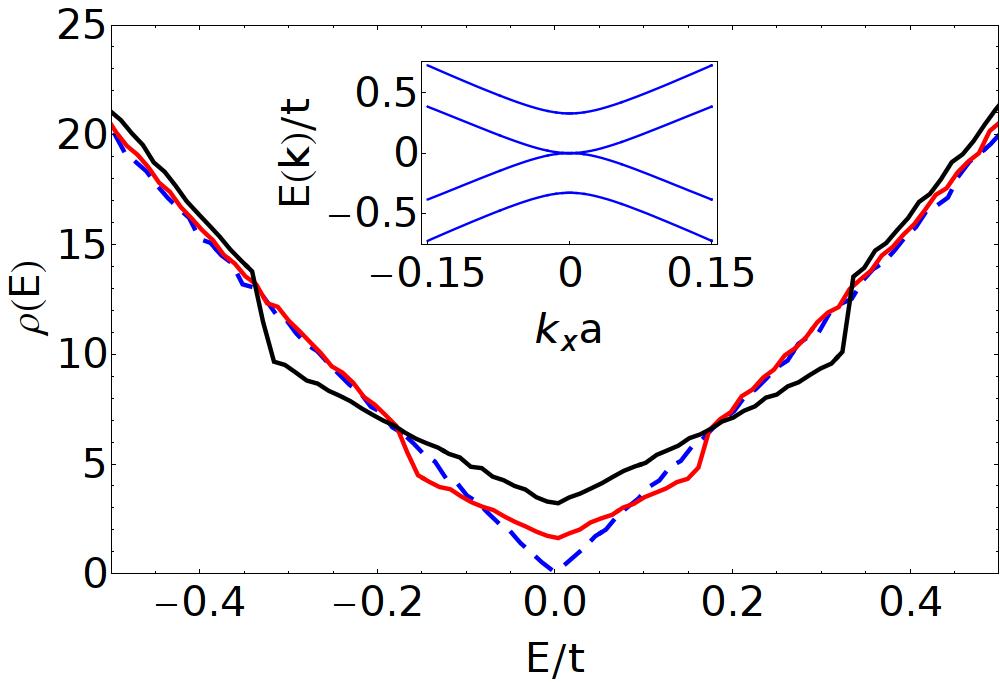
Figure 3: (Color online) Total density of states for any type II gauge field of strength $u=0.5\text{\AA}$ (red line) and $u=1\text{\AA}$ (black line), for $t=90$ meV and $t^{\prime}=0$. The unperturbed LDOS is shown as a dashed blue line for comparison. Inset: Band structure of the system for $u=1\text{\AA}$. Note the similarity with bilayer graphene.

As described in the introduction, we now consider two gauge field configurations that are not related by a gauge transformation, but whose magnetic field is the same, and consider how they should be seen in a local density of states (LDOS) measurement. Consider the type I gauge field, with a magnetic field pointing in a general direction $b^{\alpha}$ in $SU(2)$ space, $A_{i}^{\alpha}=b^{\alpha}B/2(y,-x)$. When $b^{\alpha}=(0,0,1)$ we have the usual strain induced gauge field. The case $b^{\alpha}=(0,1,0)$ was discussed in ref. GGR12, . In general, by a constant $SU(2)$ rotation of the Hamiltonian, it is not difficult to see that for any $b^{\alpha}$ the spectrum is still given by Landau levels $E_{n}=\sqrt{2Bn}$. The only difference appears in the wavefunctions, because the sublattice polarization turns out to be given by the projection of $b^{\alpha}$ onto the $z$ axis. For strain induced fields it is maximum, but for potential induced ones the density of states is in fact constant across the unit cell. One can estimate the magnetic field induced in the molecular graphene experiment with these gauge fields as follows. Take $u_{E_{1x}}=u_{max}/L*x$, with $L$ the radius of the (approximately circular) sample and $u_{max}$ the maximum displacement (at $x=L$). The magnetic field is (recovering all units)

$$B^{(x)}=\frac{\hbar/e}{\hbar v_{F}}\frac{3V^{\prime}}{4}\frac{u_{max}}{L}.$$ (13)

With $\hbar/e=6.5\cdot 10^{4}T\text{\AA}^{2}$ and taking $u_{max}=0.1a$ and $\sqrt{3}a/L\approx 1/10$ and a Fermi velocityGMK12 $\hbar v_{F}\approx 1.5\text{eV}\text{\AA}$ we obtain $B\approx 3.75T$, which is not very large compared to the strain induced one that is typically achieved.

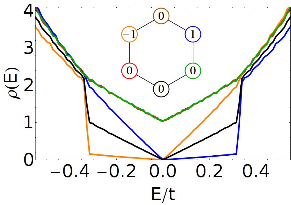
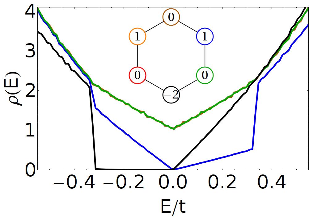
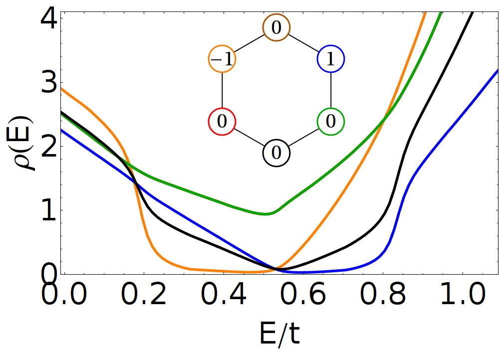
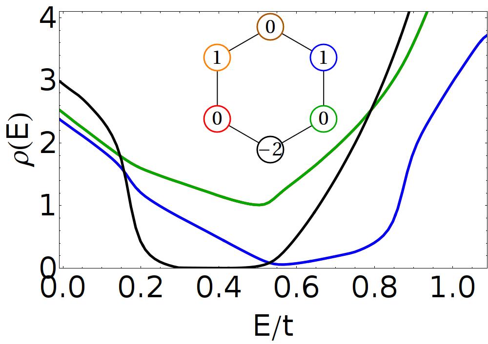
Figure 4: (color online) LDOS as a function of energy for two different gauge fields. Top left: $E_{1x}-E_{2x}$, with strength u=1 Å, $t=90$ meV and $t^{\prime}=0$. Top right: $E_{1y}-E_{2y}$, same parameters. Bottom plots are the same but with $t^{\prime}=0.18t$ and a Lorentzian broadening of $\Sigma=0.2t$. The insets show the corresponding on-site potential and the color code for the different sites within the unit cell. Note that the missing lines in the plots overlap with the line shown that has the same on-site potential.

The type II gauge field has better prospects to be experimentally accessible. Keeping $\vec{A}^{(3)}=0$, there are in fact four possible choices of constant gauge fields that give constant magnetic field, given by

$$\vec{A}^{1}=\sqrt{B/2}(1,0) \vec{A}^{2}=\sqrt{B/2}(0,\pm 1),$$ (14)

which, by eq. (12), is produced with the displacements $E_{1y}\pm E_{2y}$, and

$$\vec{A}^{1}=\sqrt{B/2}(0,1) \vec{A}^{2}=\sqrt{B/2}(\pm 1,0),$$ (15)

which is produced with the displacements $E_{1x}\pm E_{2x}$. These displacements and their on-site potentials are depicted in fig. 2. The magnetic field is given by $B=9/8(V^{\prime}u/v_{F})^{2}$ with $u=u_{E_{1i}}=\pm u_{E_{2i}}$ representing the modulus of the displacements in fig. 2. It is interesting to note that the estimate for $B$ in this case for $u=0.1a$ is $B\approx 16T$.

The Dirac Hamiltonian in the presence of these gauge fields is formally analogous to that of bilayer graphene (for a single valley), with the role of the layer played by the valley here, and an effective interlayer coupling $\gamma=\sqrt{2B}$. The spectrum of these Hamiltonians is well known to be a quadratic band touching, with two extra parabolic bands at higher energies.

Considering first the case $t^{\prime}=0$, the density of states (DOS) of this system is finite at the touching point $E_{D}=0$, and has a jump at $\pm v_{F}\sqrt{2B}=3/2V^{\prime}u$, as depicted in fig. 3. Considering a displacement $u=0.1a=1\text{\AA}$, the kink in the LDOS should appear at $\pm\text{30 meV}$, which should be easily observable. The precise location of this jump should serve as an independent estimate of the parameter $V^{\prime}$. The main effect of a finite $t^{\prime}$ is to shift $E_{D}$ to a higher value, as we will see below.

Moreover, this type of gauge field shows more complicated local density of states across the enlarged unit cell. In fig. 4 we show the LDOS for the cases $E_{1x}-E_{2x}$ and $E_{1y}-E_{2y}$. The other two combinations are obtained by mirror symmetry. For $t^{\prime}=0$, we observe different local gaps for different sites, and finite LDOS at $E=0$. For more faithful comparison with the experiment, we have also plotted the LDOS for $t^{\prime}=0.18t$, and with a Lorentzian broadening of $\Sigma=0.2t$. We observe the main effect of a shift in $E_{D}$, as well as some electron-hole assymmetry, but the main features that characterize the non-abelian gauge field remain. The identification of these features in an STM measurement would represent a demonstration of the presence of the type II constant non-abelian gauge field.

IV Discussion

In this work we have shown, by means of a symmetry analysis, how non-abelian gauge fields may be implemented in molecular graphene, and what their experimental signatures should be in the LDOS. For type I gauge fields of constant magnetic field, we have shown that because of the different microscopic origin of gauge fields $A^{(3)}$ (hopping change) and $A^{(1,2)}$ (potential change), the magnetic field that one gets in the second case is relatively smaller. While this may make the Landau level spectrum more difficult to observe, the presence of this type of field could also be readily detected, for example, in a quantum interference experiment in the weak field limit JCV11 .

We have also shown that type II constant non-abelian gauge fields generate a quadratic band touching analogous to bilayer graphene. Because of the enhanced DOS at the Fermi level, the electron-electron interaction is known to drive this system to a broken symmetry state whose precise characteristics are still controversial WAF10 ; MEM11 ; VJB12 . In the current molecular graphene experiment, the Coulomb interaction is screened by the metallic bulk, leaving residual Hubbard interactions estimated to be $U\sim 0.5t\sim 50$ meV (see Supplementary Material of ref. GMK12, ). While an ideal quadratic touching is unstable to infinitesimal short range interactions, the current broadening due to bulk tunneling ($\sim 0.2t$) is perhaps too large and may challenge the observation of the interaction induced transition. Both bulk tunneling and screening could be reduced by performing future experiments in bulk insulators with metallic surfaces (such as the recently discovered topological insulatorsHK10 ) which may eventually allow to study the fate of the many body state with a tunable analog of the interlayer hopping. Incidentally, it is also interesting to note that this instability can be interpreted as a non-abelian magnetic catalysis, where an infinitesimal field drives chiral symmetry breaking GHS98 . Furthermore, the controlled simulation of these non-abelian gauge fields, when made position dependent, may be used to study the generation of zero-energy flat bands, as those observed in the twisted bilayer system SGG12 , or the physics of topological defects in the gauge fieldGGR12 .

In summary, the molecular graphene experiment has great potential to observe many interesting phenomena related to non-abelian gauge fields with an unprecedent tunability, and which, as we have shown, should be realizable in the current experimental samples.

V Acknowledgements

I would like to thank D. Rastawiki, V. Juricic, H. Ochoa, A. G. Grushin and H. Manoharan for useful discussions. Funding from the “Programa Nacional de Movilidad de Recursos Humanos” (Spanish MECD) is acknowledged.

VI Appendix

VI.1 Estimate of V’

The parameter $V^{\prime}$ describes the change of on-site potential due to the displacements of neighbouring $CO$ molecules. As such, it is featured both in the non abelian gauge fields (which come from ”optical“ displacements) and in the strain-induced scalar potential $\phi$ (which comes from ”acoustical“ displacements). The scalar potential $\phi$ also has a contribution from NNN hopping change $\partial t^{\prime}/\partial a$ but it is much smaller and will be neglected.

To see this, consider an isotropic expansion of the $CO$ lattice. For every carbon site $i$, the induced potential is given by eq. (4). Because displacement is smooth we may write

$$V_{\vec{x}}= V^{\prime}\sum_{m}\delta_{m}^{i}r^{i}_{x+\delta_{m},CO}\approx V^{\prime}\sum_{m}\delta_{m}^{i}\frac{\delta_{m}^{j}\partial^{j}r^{i}_{x,CO}}{a}$$

$$= \frac{3a}{2}V^{\prime}(u_{xx}+u_{yy}),$$ (16)

and plugging directly into the TB Hamiltonian eq. (5), we obtain that $\phi=3V^{\prime}a/2(u_{xx}+u_{yy})$. Now consider the p-n-p juntion experiment in ref. GMK12, . The middle region is strained from $d=17.8$ to $d=20.4$ so $u_{xx}=u_{yy}=0.14$. The change in scalar potential $\Delta\phi$ is 95 meV, so we obtain ($d=\sqrt{3}a$)

$$V^{\prime}=\frac{95\text{meV}}{0.14\sqrt{3}\;17.8\text{\AA}}=22\;\text{meV}/\text{\AA}.$$ (17)

A different estimate can be obtained from the nearly free electron model considered in ref GMK12, (supp. mat.), where the scalar potential is

$$H=\frac{8\pi^{2}}{9d^{2}m}(u_{xx}+u_{yy})=\frac{3a}{2}V^{\prime}(u_{xx}+u_{yy}),$$ (18)

which gives $V^{\prime}=24\;\text{meV}/\text{\AA}$

VI.2 Symmetry of hopping perturbations

There are 9 independent hoppings in the tripled unit cell, which can be decomposed into combinations that have well defined transformation properties under the symmetries of the lattice. The 9 combinations and their symmetry labels are shown in fig. 5. In the first row, one may identify the constant hopping ($A_{1}$), the $E_{2}$ pattern that gives rise to the usual gauge field, and the Kekulé distortions (any of the three domains can be obtained from these).

The four combinations in the second row are $E_{1}$ and $E_{2}$ (and form the representation $G^{\prime}$ when the enlarged group $C_{6v}^{\prime\prime}$ is considered). These hopping patterns are produced by the same $CO$ displacements that give the non-abelian gauge fields through charge modulation. In the main part of the text we claimed that these hopping distortions cannot couple to the low energy theory around the $K$ point. The reason is simply that there is no valley off-diagonal $E_{1}$ or $E_{2}$ matrix in the low energy theory whose microscopic origin is a hopping change. This can be seen directly by inspection of table 1, where the valley mixing $E_{1}$ and $E_{2}$ matrices are all diagonal in sublattice. The hopping modulations will only appear in the low-energy theory if terms with higher order in momentum are considered. If one is interested in the whole band structure and not just low energies, these distortions in the hopping should be included by changing the NN hopping in the usual manner.

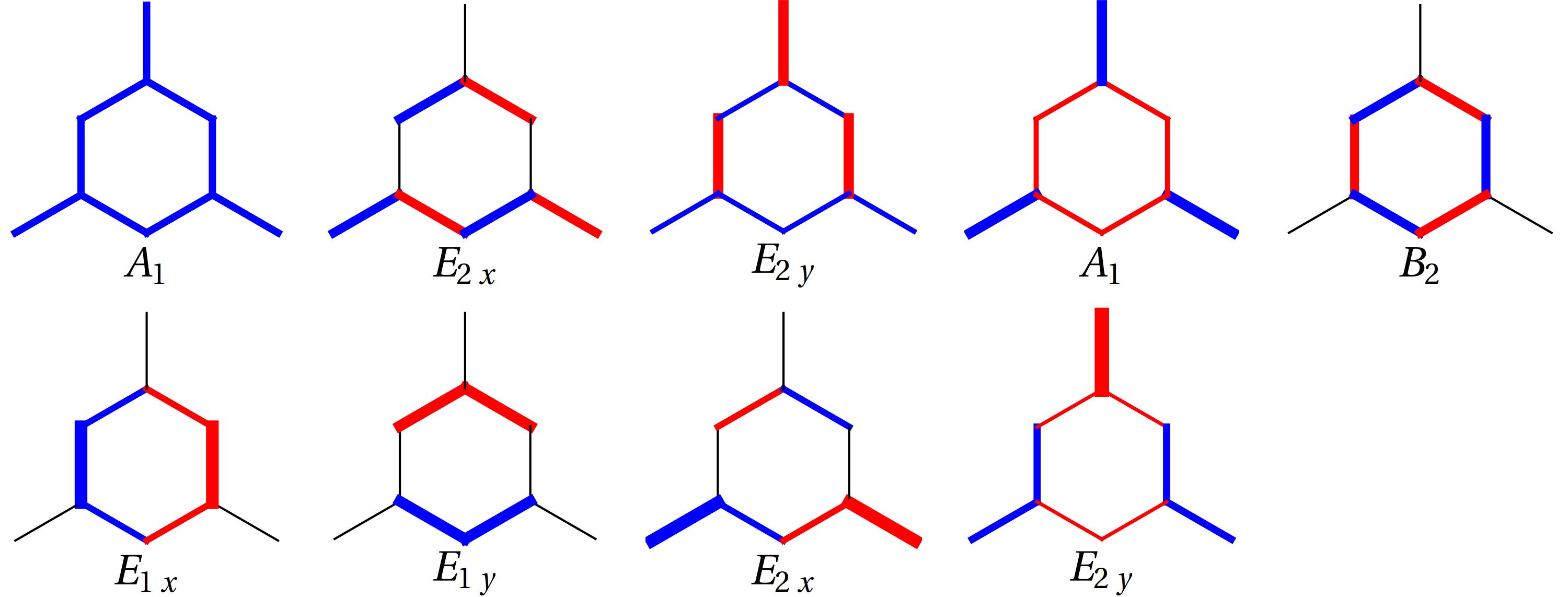
Figure 5: (Color online) The 9 independent hopping patterns and their symmetry labels. Blue means positive and red negative, and black lines represent no change in the hopping. Hopping modulations of the corresponding symmetry may also be induced by these displacements (red is negative hopping and blue is positive. However, these particular patterns have no effect in the low energy theory: they do not affect the quadratic touching and the LDOS predictions around $E=E_{D}$.

References

- (1) A. H. Castro Neto, F. Guinea, N. M. R. Peres, K. S. Novoselov, and A. K. Geim, Rev. Mod. Phys. 81, 109 (2009)
- (2) M. Z. Hasan and C. L. Kane, Rev. Mod. Phys. 82, 3045 (Nov 2010)
- (3) M. A. H. Vozmediano, M. I. Katsnelson, and F. Guinea, Physics Reports 496, 109 (2010)
- (4) V. M. Pereira and A. H. Castro Neto, Phys. Rev. Lett. 103, 046801 (2009)
- (5) F. Guinea, M. I. Katsnelson, and A. K. Geim, Nat. Phys. 6, 30 (2010)
- (6) F. de Juan, A. Cortijo, M. A. H. Vozmediano, and A. Cano, Nat. Phys. 7, 810 (2011)
- (7) N. Levy, S. A. Burke, K. L. Meaker, M. Panlasigui, A. Zettl, F. Guinea, A. H. Castro Neto, and M. F. Crommie, Science 329, 544 (2010)
- (8) C.-H. Park and S. G. Louie, Nano Letters 9, 1793 (2009)
- (9) M. Gibertini, A. Singha, V. Pellegrini, M. Polini, G. Vignale, A. Pinczuk, L. N. Pfeiffer, and K. W. West, Phys. Rev. B 79, 241406 (2009)
- (10) A. Singha, M. Gibertini, B. Karmakar, S. Yuan, M. Polini, G. Vignale, M. I. Katsnelson, A. Pinczuk, L. N. Pfeiffer, K. W. West, and V. Pellegrini, Science 332, 1176 (2011)
- (11) K. K. Gomes, W. Mar, W. Ko, F. Guinea, and H. C. Manoharan, Nature 483, 306 (2012)
- (12) C.-Y. Hou, C. Chamon, and C. Mudry, Phys. Rev. Lett. 98, 186809 (2007)
- (13) D. L. Bergman, arxiv:1205.4731(2012)
- (14) P. Ghaemi, S. Gopalakrishnan, and T. L. Hughes, arxiv:1205.4728(2012)
- (15) S. Gopalakrishnan, P. Ghaemi, and S. Ryu, Phys. Rev. B 86, 081403 (2012)
- (16) J. González, F. Guinea, and M. Vozmediano, Nuclear Physics B 406, 771 (1993)
- (17) R. T. Weitz, M. T. Allen, B. E. Feldman, J. Martin, and A. Yacoby, Science 330, 812 (2010)
- (18) A. S. Mayorov, D. C. Elias, M. Mucha-Kruczynski, R. V. Gorbachev, T. Tudorovskiy, A. Zhukov, S. V. Morozov, M. I. Katsnelson, V. I. Fal’ko, A. K. Geim, and K. S. Novoselov, Science 333, 860 (2011)
- (19) J. Velasco, L. Jing, W. Bao, Y. Lee, P. Kratz, V. Aji, M. Bockrath, C. N. Lau, C. Varma, R. Stillwell, D. Smirnov, F. Zhang, J. Jung, and A. H. MacDonald, Nat. Nanotech. 7, 156 (2012)
- (20) J. Fröhlich and U. M. Studer, Rev. Mod. Phys. 65, 733 (1993)
- (21) I. V. Tokatly, Phys. Rev. Lett. 101, 106601 (2008)
- (22) F. Wilczek and A. Zee, Phys. Rev. Lett. 52, 2111 (1984)
- (23) K. Osterloh, M. Baig, L. Santos, P. Zoller, and M. Lewenstein, Phys. Rev. Lett. 95, 010403 (2005)
- (24) J. Ruseckas, G. Juzeliūnas, P. Öhberg, and M. Fleischhauer, Phys. Rev. Lett. 95, 010404 (2005)
- (25) J. Dalibard, F. Gerbier, G. Juzeliūnas, and P. Öhberg, Rev. Mod. Phys. 83, 1523 (2011)
- (26) P. San-Jose, J. González, and F. Guinea, Phys. Rev. Lett. 108, 216802 (2012)
- (27) T. T. Wu and C. N. Yang, Phys. Rev. D 12, 3843 (1975)
- (28) M. H. Friedman, Y. Srivastava, and A. Widom, J. Phys. G: Nucl. Part. Phys. 23, 1061 (1997)
- (29) The resolution to this apparent paradox is simply that for non-abelian fields there are further independent gauge invariant quantities, such as , that distinguish among them.
- (30) D. M. Basko, Phys. Rev. B 78, 125418 (Sep 2008)
- (31) J. L. Mañes, Phys. Rev. B 76, 045430 (2007)
- (32) R. Winkler and U. Zülicke, Phys. Rev. B 82, 245313 (2010)
- (33) T. L. Linnik, J. Phys.: Cond. Mat. 24, 205302 (2012)
- (34) R. Ferone, J. R. Wallbank, V. Zólyomi, E. McCann, and V. I. Fal’ko, Solid State Comm. 151, 1071 (2011)
- (35) O. Pankratov, S. Hensel, and M. Bockstedte, Phys. Rev. B 82, 121416 (Sep 2010)
- (36) Or to the Dirac Hamiltonian in the presence of Rashba spin-orbit coupling. Not surprisingly these Hamiltonians are described in terms of SU(2) gauge fields too.
- (37) V. P. Gusynin, D. K. Hong, and I. A. Shovkovy, Phys. Rev. D 57, 5230 (1998)