Maxwell Demon from a
Quantum Bayesian Networks
Perspective

Abstract

We propose a new inequality that we call the conditional ageing inequality (CAIN). The CAIN is a slight generalization to non-equilibrium situations of the Second Law of thermodynamics. The goal of this paper is to study the consequences of the CAIN. We use the CAIN to discuss Maxwell demon processes (i.e., thermodynamic processes with feedback.) In particular, we apply the CAIN to four cases of the Szilard engine: for a classical or a quantum system with either one or two correlated particles. Besides proposing this new inequality that we call the CAIN, another novel feature of this paper is that we use quantum Bayesian networks for our analysis of Maxwell demon processes.

1 Introduction

In Ref.[1], Maxwell proposed his famous gedanken experiment wherein a demon controls the flow of gas particles from one chamber to another and decides which particles to let through based on their temperature. He gave this thought experiment as an example of a thermodynamic process in which the Second Law of thermodynamics appears to be violated. He dismissed the paradox by saying that the Second Law is true only on average. In Ref.[2], Szilard proposed an engine which is a simplified version of a Maxwell’s demon. Szilard argued that for his engine, the Second Law is not violated at all, as long as the work performed by the demon to make his measurements is taken into account. In Refs.[3] and [4], Landauer and later Bennett pointed out that measurements can be performed without spending any energy, but that in order for an engine to perform a cyclic process, it needs to store the information of the measurement on a tape and then erase and re-initialize that tape once per cycle. These tape operations will always consume an amount of energy larger or equal to the work the demon can extract from changes in gas volumes.

Maxwell’s demon thought experiment might have once been considered paradoxical, but after the work of Szilard, Landauer and Bennett, most scientists consider the paradox pretty much solved. Nevertheless, some people, myself included, still strive to make the mathematics involved in the treatment of Maxwell’s demon a bit more streamlined. That is one of the goals of this paper, to look at Maxwell’s demon from a different point of view, hoping that this might yield new insights to an already understood problem.

This paper originated as an attempt to understand a series of papers (Refs.[5] to [11]) by Sagawa, Ueda and coworkers (S-U) in which they claim that the standard Second Law of thermodynamics does not apply to non-equilibrium processes with feedback (i.e., Maxwell demon type processes). They give a generalization of the Second Law that they claim does apply to such processes. Although I agree in spirit with much of what S-U are trying to do, and I profited immensely from reading their papers, I disagree with some of the details of their theory. I discuss my disagreements with the S-U theory in a separate paper, Ref.[12]. The goal of this paper is to report on my own theory for generalizing the Second Law so that is applies to processes with feedback. My theory agrees in spirit with the S-U theory, but differs from it in some important details.

Let me explain the rationale behind my theory.

Suppose we want to consider a system in thermal contact but not necessarily in equilibrium with a bath at temperature $T$. Let ${\,\underline{X}\,}$ denote all non-thermal variables (fast changing, not in thermal equilibrium) and let ${\,\underline{\Theta}\,}$ denote all thermal variables (slow changing, in thermal equilibrium) describing both the system and bath. Let $\tau$ denote time. For any operator $\Omega_{\tau}$, define $\Omega_{\tau}{|_{\tau=\tau_{1}}^{\tau_{2}}}=\Omega_{\tau_{2}}-\Omega_{\tau_{1}}$. My slight generalization of the Second Law is

$$\framebox{$\displaystyle\;\;S_{\tau}({\,\underline{\Theta}\,}_{\tau}|{\,\underline{X}\,}_{\tau}){|_{\tau=0}^{\tau}}\geq 0\;\;$}\;,$$ (1)

where $S({\,\underline{a}\,}|{\,\underline{b}\,})$ is the conditional entropy (i.e., conditional spread) of ${\,\underline{a}\,}$ given ${\,\underline{b}\,}$. I call Eq.(1) the conditional ageing inequality (CAIN). The standard Second Law corresponds to the special case when there are no ${\,\underline{X}\,}_{\tau}$ variables, in which case Eq.(1) reduces to

$$S_{\tau}({\,\underline{\Theta}\,}_{\tau}){|_{\tau=0}^{\tau}}\geq 0\;.$$ (2)

The standard Second Law could be described as unconditional ageing, or simply as ageing.

Now, what is the justification for the CAIN? The justification for the Second Law Eq.(2) is that the superoperator that evolves the overall probability distribution in the classical case (or the overall density matrix in the quantum case), from time 0 to $\tau$, increases entropy because it can be shown to be doubly stochastic in the classical case (or unital in the quantum case). The justification for the CAIN is the same, except that the evolution superoperator is doubly stochastic (or unital) only if the non-thermal variables are held fixed during the evolution. The CAIN is not true for all evolution superoperators. Our hope is that it applies to systems of interest that commonly occur in nature.

The goal of this paper is to study the consequences of the CAIN. In particular, we apply the CAIN to four cases of the Szilard engine: for a classical or a quantum system with either one or two correlated particles.

Besides proposing this new inequality that we call the CAIN, another novel feature of this paper is that we use quantum Bayesian networks for our analysis of Maxwell demon type processes.

This paper is written assuming that the reader has first read Refs.[13] and [14]. Ref.[13] is an introduction to quantum Bayesian networks for mixed states. Ref.[14] discusses well-known inequalities of classical and quantum SIT (Shannon Information Theory) from a Bayesian networks perspective.

In this paper, we will use the abbreviation $\frac{f(a)}{\sum_{a}(num)}=\frac{f(a)}{\sum_{a}f(a)}$. We will also use the abbreviations $\Gamma_{a\;:\;b}=(\Gamma_{a},\Gamma_{a+1},\Gamma_{a+2},\ldots,\Gamma_{b})$ and $\Gamma_{<b}=\Gamma_{0\;:\;b}$, for any vector $\Gamma_{a}$ and any integers $a,b$ such that $0\leq a\leq b$.

2 Review of Some Properties of
Thermal States

In this section, we will review some well known properties of thermal states that we shall use later on in the paper to study some consequences of the CAIN. Most of the contents of this section can be found in reviews about entropy such as Ref.[15] by Wehrl and textbooks on Statistical Mechanics such as Ref.[16] by Feynman.

Suppose ${\,\underline{j}\,}$ is a classical random variable that can take on values $j\in S_{\,\underline{j}\,}$ and has a probability distribution $P_{\,\underline{j}\,}(j)$. We will denote the average of any function $f:S_{\,\underline{j}\,}\rightarrow{\mathbb{R}}$ by

$$\left\langle f(j)\right\rangle_{j}=\left\langle f(j)\right\rangle_{P_{\,\underline{j}\,}}=\sum_{j}P(j)f(j)\;.$$ (3)

When speaking about quantum physics, if $\rho$ is a density operator acting on a Hilbert space ${\cal H}$, and $\Omega$ is a Hermitian operator also acting on ${\cal H}$, we will denote the average of $\Omega$ by

$$\left\langle\Omega\right\rangle_{\rho}={\rm tr}(\rho\Omega)\;.$$ (4)

For example, in this notation the von Neumann entropy of $\rho$ is

$$S(\rho)=-\left\langle\ln\rho\right\rangle_{\rho}\;.$$ (5)

Consider a system with density matrix $\rho$ and Hamiltonian ${\hat{\scriptstyle E}}$. Suppose the eigenvalue decomposition of ${\hat{\scriptstyle E}}$ is ${\hat{\scriptstyle E}}=\sum_{j}P(j)|E_{j}\rangle\langle E_{j}|$. The internal energy of the system is defined as

$$U=E=\left\langle{\hat{\scriptstyle E}}\right\rangle_{\rho}=\left\langle E_{j}\right\rangle_{j}\;.$$ (6)

2.1 Simple Properties of Thermal States

Thermal states (a.k.a canonical ensemble or Gibbs states) are states with a definite temperature $T$. Their form is given below.

In this paper, we will use what are called natural Planck units. As in Eq.(5), our entropies will be defined in terms of natural logs (instead of base 2 logs) and without the $k_{B}$. ($k_{B}$ is Boltzmann’s constant.) Temperatures will be given in energy units and entropies in nats. If $T$ is the temperature in energy units and $T^{Kel}$ is the temperature in degrees Kelvin, then $T=k_{B}T^{Kel}$. We will also use $\beta=\frac{1}{T}$.

Consider a system with Hamiltonian ${\hat{\scriptstyle E}}=\sum_{j}P(j)|E_{j}\rangle\langle E_{j}|$. which has reached thermal equilibrium at a temperature $T$. The partition function of the system is defined by

$$Z^{\beta}({\hat{\scriptstyle E}})={\rm tr}(e^{-\beta{\hat{\scriptstyle E}}})=\sum_{j}e^{-\beta E_{j}}\;.$$ (7)

Its density matrix is

$$\rho^{\beta}({\hat{\scriptstyle E}})=\frac{R}{Z^{\beta}({\hat{\scriptstyle E}})}\;,\mbox{ where }R=e^{-\beta{\hat{\scriptstyle E}}}\;.$$ (8)

Its entropy is

$$S^{\beta}({\hat{\scriptstyle E}})=S(\rho^{\beta}({\hat{\scriptstyle E}}))\;.$$ (9)

Its free energy is

$$F^{\beta}({\hat{\scriptstyle E}})=-T\ln Z^{\beta}({\hat{\scriptstyle E}})\;.$$ (10)

Its pressure $P$ (not to be confused with probability $P(j)$) is

$$P=-\left\langle\left(\frac{\partial E_{j}}{\partial V}\right)_{T}\right\rangle_{j}\;.$$ (11)

Later we will show that this expression for pressure gives the expected $dE=-PdV$ (Thus, internal energy of system decreases if system does work by increasing its volume by $dV$).

Claim 1

Let $S=S^{\beta}({\hat{\scriptstyle E}})$, $E=\left\langle{\hat{\scriptstyle E}}\right\rangle_{\rho^{\beta}({\hat{\scriptstyle E}})}$, and $F=F^{\beta}({\hat{\scriptstyle E}})$. Then

$$E=TS+F\;.$$ (12a)

(Thus, internal energy is sum of bound part ($$T$$ times entropy) and free part (free energy)). Furthermore

$$\left(\frac{\partial F}{\partial V}\right)_{T}=-P,\;\;\left(\frac{\partial F}{\partial T}\right)_{V}=-S\;.$$ (12b)

(Thus, free energy decreases if volume or temperature increase). Furthermore

$$dF=-SdT-PdV\;,$$ (12c)

and

$$dE=TdS-PdV\;.$$ (12d)

proof:

To prove Eq.(12a), note that

$$S=\left\langle\ln\frac{Z}{e^{-\beta E_{j}}}\right\rangle_{j}=\ln Z+\beta\left\langle E_{j}\right\rangle_{j}=-\frac{F}{T}+\frac{E}{T}\;.$$ (13)

To prove Eq.(12b), note that

$$\left(\frac{\partial F}{\partial V}\right)_{T}=-T\left(\frac{\partial\ln Z}{\partial V}\right)_{T}=\frac{-T}{Z}\sum_{j}(-\beta e^{-\beta E_{j}})\left(\frac{\partial E_{j}}{\partial V}\right)_{T}=-P\;.$$ (14)

$$\left(\frac{\partial F}{\partial T}\right)_{V} = -\ln Z-\frac{T}{Z}\left(\frac{\partial Z}{\partial T}\right)_{V}$$ (15a)

$$= -\ln Z+\beta\left(\frac{\partial\ln Z}{\partial\beta}\right)_{V}$$ (15b)

$$= -\ln Z-E\beta=-S\;.$$ (15c)

To prove Eq.(12c), note that

$$dF=\left(\frac{\partial F}{\partial V}\right)_{T}dV+\left(\frac{\partial F}{\partial T}\right)_{V}dT\;.$$ (16)

To prove Eq.(12d), just use Eqs.(12a) and (12c).
QED

Claim 2

$S^{\beta}({\hat{\scriptstyle E}})$ and $\left\langle{\hat{\scriptstyle E}}\right\rangle_{\rho^{\beta}({\hat{\scriptstyle E}})}$ are monotonically increasing and $F^{\beta}({\hat{\scriptstyle E}})$ is monotonically decreasing functions of temperature. In fact,

$$-\frac{dS(\rho)}{\beta d\beta}=-\frac{d\left\langle{\hat{\scriptstyle E}}\right\rangle_{\rho}}{d\beta}=\left\langle({\hat{\scriptstyle E}}-\left\langle{\hat{\scriptstyle E}}\right\rangle_{\rho})^{2}\right\rangle_{\rho}\geq 0\;,$$ (17)

and

$$\frac{dF^{\beta}({\hat{\scriptstyle E}})}{d\beta}=\frac{S(\rho)}{\beta^{2}}\;,$$ (18)

where we are abbreviating $\rho^{\beta}({\hat{\scriptstyle E}})$ by just $\rho$.

proof: Just straightforward Calculus.
QED

Claim 3

Let $S=S^{\beta}({\hat{\scriptstyle E}})$, $E=\left\langle{\hat{\scriptstyle E}}\right\rangle_{\rho^{\beta}({\hat{\scriptstyle E}})}$, and $F=F^{\beta}({\hat{\scriptstyle E}})$. Then

$$\begin{array}[]{|c|c|c|}\hline\cr&T\rightarrow 0&T\rightarrow\infty\\ \hline\cr\hline\cr S=&0&\ln N\\ \hline\cr E=&E_{0}&\frac{1}{N}\sum_{j}E_{j}\\ \hline\cr F=&E_{0}&-T\ln N\\ \hline\cr\end{array}\;,$$ (19)

where $\{E_{j}\}_{j=0}^{N-1}$ are the eigenvalues of ${\hat{\scriptstyle E}}$ and $E_{0}$ is the lowest one.

proof: Obvious.
QED

2.2 Inequalities Relating a Thermal State With a Neighboring State

Consider any Hilbert space ${\cal H}$, any density matrix $\rho$ acting on ${\cal H}$, any Hamiltonian ${\hat{\scriptstyle E}}$ acting on ${\cal H}$, and any temperature $T$. Define

$$S^{\beta}({\hat{\scriptstyle E}},\rho)=\beta[\left\langle{\hat{\scriptstyle E}}\right\rangle_{\rho}-F^{\beta}({\hat{\scriptstyle E}})]\;$$ (20)

and

$$F^{\beta}({\hat{\scriptstyle E}},\rho)=\left\langle{\hat{\scriptstyle E}}\right\rangle_{\rho}-TS(\rho)\;.$$ (21)

I will refer these functions as the $S$ and $F$ capping functions, respectively, because, as we will prove later, they are upper bounds to their namesakes.

It’s easy to check that $S^{\beta}({\hat{\scriptstyle E}},\rho^{\beta}({\hat{\scriptstyle E}}))=S^{\beta}({\hat{\scriptstyle E}})$ and $F^{\beta}({\hat{\scriptstyle E}},\rho^{\beta}({\hat{\scriptstyle E}}))=F^{\beta}({\hat{\scriptstyle E}})$.

Claim 4

$$D(\rho//\rho^{\beta}({\hat{\scriptstyle E}})) = S^{\beta}({\hat{\scriptstyle E}},\rho)-S(\rho)$$ (22a)

$$= \beta[F^{\beta}({\hat{\scriptstyle E}},\rho)-F^{\beta}({\hat{\scriptstyle E}})]\;.$$ (22b)

proof:

$$D(\rho//\rho^{\beta}({\hat{\scriptstyle E}})) = \left\langle\ln\rho-\ln\rho^{\beta}({\hat{\scriptstyle E}})\right\rangle_{\rho}$$ (23a)

$$= \beta[-TS(\rho)+\left\langle{\hat{\scriptstyle E}}\right\rangle_{\rho}-F^{\beta}({\hat{\scriptstyle E}})]$$ (23b)

$$= S^{\beta}({\hat{\scriptstyle E}},\rho)-S(\rho)$$ (23c)

$$= \beta[F^{\beta}({\hat{\scriptstyle E}},\rho)-F^{\beta}({\hat{\scriptstyle E}})]\;.$$ (23d)

QED

Claim 5

$$S(\rho)\leq S^{\beta}({\hat{\scriptstyle E}},\rho)\;.$$ (24)

If $\left\langle{\hat{\scriptstyle E}}\right\rangle_{\rho}\leq\left\langle{\hat{\scriptstyle E}}\right\rangle_{\rho^{\beta}({\hat{\scriptstyle E}})}$, then also

$$S(\rho)\leq S^{\beta}({\hat{\scriptstyle E}})\;.$$ (25)

(Eq.(25) agrees with our intuition that $\left\langle{\hat{\scriptstyle E}}\right\rangle_{\rho}$ and $S(\rho)$ both measure the energy spread of $\rho$.)

proof: Eq.(24) follows from Eq.(22a).

If $\left\langle{\hat{\scriptstyle E}}\right\rangle_{\rho}\leq\left\langle{\hat{\scriptstyle E}}\right\rangle_{\rho^{\beta}({\hat{\scriptstyle E}})}$, then

$$S(\rho) \leq \beta[\left\langle{\hat{\scriptstyle E}}\right\rangle_{\rho}-F^{\beta}({\hat{\scriptstyle E}})]$$ (26a)

$$\leq \beta[\left\langle{\hat{\scriptstyle E}}\right\rangle_{\rho^{\beta}({\hat{\scriptstyle E}})}-F^{\beta}({\hat{\scriptstyle E}})]$$ (26b)

$$= S^{\beta}({\hat{\scriptstyle E}})\;.$$ (26c)

QED

Claim 6

$$F^{\beta}({\hat{\scriptstyle E}})\leq F^{\beta}({\hat{\scriptstyle E}},\rho)\;.$$ (27)

Also

$$F^{\beta}({\hat{\scriptstyle E}})\leq\left\langle{\hat{\scriptstyle E}}\right\rangle_{\rho}\;.$$ (28)

Thus, the free energy is always less than the average energy. (There is no free lunch.)

proof: Eq.(27) follows from Eq.(22b).

Eq.(28) follows from Eq.(24) and the definition of $S^{\beta}({\hat{\scriptstyle E}},\rho)$.
QED

Suppose ${\hat{\scriptstyle E}}_{1}$ and ${\hat{\scriptstyle E}}_{2}$ are two Hamiltonians acting on the same Hilbert space. If $[{\hat{\scriptstyle E}}_{1},{\hat{\scriptstyle E}}_{2}]=0$, then clearly $Z^{\beta}({\hat{\scriptstyle E}}_{1}+{\hat{\scriptstyle E}}_{2})=Z^{\beta}({\hat{\scriptstyle E}}_{1})Z^{\beta}({\hat{\scriptstyle E}}_{2})$ so $F^{\beta}({\hat{\scriptstyle E}}_{1}+{\hat{\scriptstyle E}}_{2})=F^{\beta}({\hat{\scriptstyle E}}_{1})+F^{\beta}({\hat{\scriptstyle E}}_{2})$. But what if ${\hat{\scriptstyle E}}_{1}$ and ${\hat{\scriptstyle E}}_{1}$ don’t commute? Is the free energy sub-additive or super-additive (or neither) in its Hamiltonian?

Claim 7

(Peierls-Bogoliubov)

$$F^{\beta}({\hat{\scriptstyle E}}_{2})\leq F^{\beta}({\hat{\scriptstyle E}}_{1})+\left\langle{\hat{\scriptstyle E}}_{2}-{\hat{\scriptstyle E}}_{1}\right\rangle_{\rho^{\beta}({\hat{\scriptstyle E}}_{1})}\;.$$ (29)

proof:

$$D(\rho^{\beta}({\hat{\scriptstyle E}}_{1})//\rho^{\beta}({\hat{\scriptstyle E}}_{2})) = \left\langle\ln\rho^{\beta}({\hat{\scriptstyle E}}_{1})-\ln\rho^{\beta}({\hat{\scriptstyle E}}_{2})\right\rangle_{\rho^{\beta}({\hat{\scriptstyle E}}_{1})}$$ (30a)

$$= -S^{\beta}({\hat{\scriptstyle E}}_{1})+\beta\left\langle{\hat{\scriptstyle E}}_{2}\right\rangle_{\rho^{\beta}({\hat{\scriptstyle E}}_{1})}-\beta F^{\beta}({\hat{\scriptstyle E}}_{2})$$ (30b)

$$= -S^{\beta}({\hat{\scriptstyle E}}_{1})+\beta\left\langle{\hat{\scriptstyle E}}_{1}\right\rangle_{\rho^{\beta}({\hat{\scriptstyle E}}_{1})}-\beta F^{\beta}({\hat{\scriptstyle E}}_{2})+\beta\left\langle{\hat{\scriptstyle E}}_{2}-{\hat{\scriptstyle E}}_{1}\right\rangle_{\rho^{\beta}({\hat{\scriptstyle E}}_{1})}$$ (30c)

$$= \beta[F^{\beta}({\hat{\scriptstyle E}}_{1})-F^{\beta}({\hat{\scriptstyle E}}_{2})]+\beta\left\langle{\hat{\scriptstyle E}}_{2}-{\hat{\scriptstyle E}}_{1}\right\rangle_{\rho^{\beta}({\hat{\scriptstyle E}}_{1})}\;.$$ (30d)

QED

Claim 8

$$F^{\beta}({\hat{\scriptstyle E}})+\left\langle\Delta{\hat{\scriptstyle E}}\right\rangle_{\rho({\hat{\scriptstyle E}}+\Delta{\hat{\scriptstyle E}})}\stackrel{{\scriptstyle(a)}}{{\leq}}F({\hat{\scriptstyle E}}+\Delta{\hat{\scriptstyle E}})\stackrel{{\scriptstyle(b)}}{{\leq}}F^{\beta}({\hat{\scriptstyle E}})+\left\langle\Delta{\hat{\scriptstyle E}}\right\rangle_{\rho({\hat{\scriptstyle E}})}\;.$$ (31)

proof:

Inequality $(a)$ follows if one sets ${\hat{\scriptstyle E}}_{1}={\hat{\scriptstyle E}}+\Delta{\hat{\scriptstyle E}}$ and ${\hat{\scriptstyle E}}_{2}={\hat{\scriptstyle E}}$ in Eq.(29).

Inequality $(b)$ follows if one sets ${\hat{\scriptstyle E}}_{1}={\hat{\scriptstyle E}}$ and ${\hat{\scriptstyle E}}_{2}={\hat{\scriptstyle E}}+\Delta{\hat{\scriptstyle E}}$ in Eq.(29).
QED

Claim 9

$$F^{\beta}({\hat{\scriptstyle E}})+F^{\beta}(\Delta{\hat{\scriptstyle E}})\leq F^{\beta}({\hat{\scriptstyle E}}+\Delta{\hat{\scriptstyle E}})\;.$$ (32)

proof: Just use the no-free lunch inequality in Eq.(31) side $(a)$.
QED

3 The Conditional Ageing Inequality and Some of its Consequences

In Appendix A, we reminded the reader of the well know inequality $dW_{s}\leq-dF_{s}$, which says that at fixed temperature, the drop in free energy is an upper bound to the amount of work system $s$ can do. In this section we apply the conditional ageing inequality to find: a lower bound on $-dF_{X}$ for a system ${\,\underline{X}\,}$ in contact with a heat reservoir ${\,\underline{\Theta}\,}$ at temperature $T$.

We will abbreviate $\rho_{\tau;{\,\underline{\Theta}\,}_{\tau},{\,\underline{X}\,}_{\tau}}$ by $\rho_{\tau}$. The partial traces of $\rho_{\tau;{\,\underline{\Theta}\,}_{\tau},{\,\underline{X}\,}_{\tau}}$ will be denoted by $\rho_{\tau;{\,\underline{\Theta}\,}_{\tau}}$ and $\rho_{\tau;{\,\underline{X}\,}_{\tau}}$. We will also abbreviate $S_{\tau}(\cdot)=S_{\rho_{\tau;{\,\underline{\Theta}\,}_{\tau},{\,\underline{X}\,}_{\tau}}}(\cdot)$ for any argument $(\cdot)$.

Let the joint system of ${\,\underline{X}\,}$ and ${\,\underline{\Theta}\,}$ have as Hamiltonian

$${\hat{\scriptstyle E}}_{{\,\underline{\Theta}\,}_{\tau},{\,\underline{X}\,}_{\tau}}={\hat{\scriptstyle E}}_{{\,\underline{X}\,}_{\tau}}+{\hat{\scriptstyle E}}_{{\,\underline{\Theta}\,}_{\tau}}+\epsilon_{{\,\underline{\Theta}\,}_{\tau},{\,\underline{X}\,}_{\tau}}={\hat{\scriptstyle E}}_{{\,\underline{X}\,}_{\tau}}+\Delta{\hat{\scriptstyle E}}_{{\,\underline{\Theta}\,}_{\tau},{\,\underline{X}\,}_{\tau}}\;,$$ (33)

where $[{\hat{\scriptstyle E}}_{{\,\underline{X}\,}_{\tau}},{\hat{\scriptstyle E}}_{{\,\underline{\Theta}\,}_{\tau}}]=0$ and $\epsilon_{{\,\underline{\Theta}\,}_{\tau},{\,\underline{X}\,}_{\tau}}$ is small.

The conditional ageing inequality (CAIN) is

$$S_{\tau}({\,\underline{\Theta}\,}_{\tau}|{\,\underline{X}\,}_{\tau}){|_{\tau=0}^{\tau}}\geq 0\;.$$ (34)

Besides the CAIN, we will also assume that the following is true at $\tau=0$: ${\,\underline{\Theta}\,}_{0}$ and ${\,\underline{X}\,}_{0}$ are independent and thermal. The independence is achieved by assuming that $\epsilon_{{\,\underline{\Theta}\,}_{0},{\,\underline{X}\,}_{0}}=0$.

Claim 10

If the CAIN holds, and ${\,\underline{\Theta}\,}_{0}$ and ${\,\underline{X}\,}_{0}$ are independent and thermal, then

$$-F^{\beta}({\hat{\scriptstyle E}}_{{\,\underline{X}\,}_{\tau}},\rho_{\tau;{\,\underline{X}\,}_{\tau}}){|_{\tau=0}^{\tau}}-TS^{\beta}(\Delta{\hat{\scriptstyle E}}_{{\,\underline{\Theta}\,}_{\tau},{\,\underline{X}\,}_{\tau}},\rho_{\tau}){|_{\tau=0}^{\tau}}\leq-F^{\beta}({\hat{\scriptstyle E}}_{{\,\underline{X}\,}_{\tau}}){|_{\tau=0}^{\tau}}\;$$ (35)

where

$$-F^{\beta}({\hat{\scriptstyle E}}_{{\,\underline{X}\,}_{\tau}})=TS^{\beta}({\hat{\scriptstyle E}}_{{\,\underline{X}\,}_{\tau}})-\left\langle{\hat{\scriptstyle E}}_{{\,\underline{X}\,}_{\tau}}\right\rangle_{\rho^{\beta}({\hat{\scriptstyle E}}_{{\,\underline{X}\,}_{\tau}})}\;$$ (36)

and

$$-F^{\beta}({\hat{\scriptstyle E}}_{{\,\underline{X}\,}_{\tau}},\rho_{\tau;{\,\underline{X}\,}_{\tau}})=TS(\rho_{\tau;{\,\underline{X}\,}_{\tau}})-\left\langle{\hat{\scriptstyle E}}_{{\,\underline{X}\,}_{\tau}}\right\rangle_{\rho_{\tau;{\,\underline{X}\,}_{\tau}}}\;.$$ (37)

proof:

The CAIN implies

$$S_{\tau}({\,\underline{X}\,}_{\tau}){|_{\tau=0}^{\tau}}\leq S_{\tau}({\,\underline{\Theta}\,}_{\tau},{\,\underline{X}\,}_{\tau}){|_{\tau=0}^{\tau}}\;.$$ (38)

But

$$S_{\tau}({\,\underline{\Theta}\,}_{\tau},{\,\underline{X}\,}_{\tau}) = S(\rho_{\tau;{\,\underline{\Theta}\,}_{\tau},{\,\underline{X}\,}_{\tau}})$$ (39a)

$$\leq \beta\left[\left\langle\Delta{\hat{\scriptstyle E}}_{{\,\underline{\Theta}\,}_{\tau},{\,\underline{X}\,}_{\tau}}+{\hat{\scriptstyle E}}_{{\,\underline{X}\,}_{\tau}}\right\rangle_{\rho_{\tau}}-F^{\beta}(\Delta{\hat{\scriptstyle E}}_{{\,\underline{\Theta}\,}_{\tau},{\,\underline{X}\,}_{\tau}}+{\hat{\scriptstyle E}}_{{\,\underline{X}\,}_{\tau}})\right]$$ (39b)

$$\leq \beta\left[\left\langle\Delta{\hat{\scriptstyle E}}_{{\,\underline{\Theta}\,}_{\tau},{\,\underline{X}\,}_{\tau}}+{\hat{\scriptstyle E}}_{{\,\underline{X}\,}_{\tau}}\right\rangle_{\rho_{\tau}}-F^{\beta}(\Delta{\hat{\scriptstyle E}}_{{\,\underline{\Theta}\,}_{\tau},{\,\underline{X}\,}_{\tau}})-F^{\beta}({\hat{\scriptstyle E}}_{{\,\underline{X}\,}_{\tau}})\right]$$ (39c)

$$= S^{\beta}(\Delta{\hat{\scriptstyle E}}_{{\,\underline{\Theta}\,}_{\tau},{\,\underline{X}\,}_{\tau}},\rho_{\tau})+S^{\beta}({\hat{\scriptstyle E}}_{{\,\underline{X}\,}_{\tau}},\rho_{\tau})\;.$$ (39d)

Also, since ${\,\underline{X}\,}_{0}$ and ${\,\underline{\Theta}\,}_{0}$ are independent and thermal,

$$S_{0}({\,\underline{\Theta}\,}_{0},{\,\underline{X}\,}_{0}) = S^{\beta}({\hat{\scriptstyle E}}_{{\,\underline{\Theta}\,}_{0}})+S^{\beta}({\hat{\scriptstyle E}}_{{\,\underline{X}\,}_{0}})$$ (40a)

$$= S^{\beta}({\hat{\scriptstyle E}}_{{\,\underline{\Theta}\,}_{0}},\rho_{0})+S^{\beta}({\hat{\scriptstyle E}}_{{\,\underline{X}\,}_{0}},\rho_{0})\;.$$ (40b)

Combining Eqs.(38), (39d) and (40b) yields

$$S(\rho_{\tau;{\,\underline{X}\,}_{\tau}}){|_{\tau=0}^{\tau}}=S_{\tau}({\,\underline{X}\,}_{\tau}){|_{\tau=0}^{\tau}}\leq S^{\beta}(\Delta{\hat{\scriptstyle E}}_{{\,\underline{\Theta}\,}_{\tau},{\,\underline{X}\,}_{\tau}},\rho_{\tau}){|_{\tau=0}^{\tau}}+S^{\beta}({\hat{\scriptstyle E}}_{{\,\underline{X}\,}_{\tau}},\rho_{\tau}){|_{\tau=0}^{\tau}}\;.$$ (41)

Now using

$$S^{\beta}({\hat{\scriptstyle E}}_{{\,\underline{X}\,}_{\tau}},\rho_{\tau}){|_{\tau=0}^{\tau}}=\beta[\left\langle{\hat{\scriptstyle E}}_{{\,\underline{X}\,}_{\tau}}\right\rangle_{\rho_{\tau}}-F^{\beta}({\hat{\scriptstyle E}}_{{\,\underline{X}\,}_{\tau}})]{|_{\tau=0}^{\tau}}\;$$ (42)

gives

$$-\beta F^{\beta}({\hat{\scriptstyle E}}_{{\,\underline{X}\,}_{\tau}},\rho_{\tau;{\,\underline{X}\,}_{\tau}}){|_{\tau=0}^{\tau}} = S(\rho_{\tau;{\,\underline{X}\,}_{\tau}}){|_{\tau=0}^{\tau}}-\beta\left\langle{\hat{\scriptstyle E}}_{{\,\underline{X}\,}_{\tau}}\right\rangle_{\rho_{\tau}}{|_{\tau=0}^{\tau}}$$ (43a)

$$\leq S^{\beta}(\Delta{\hat{\scriptstyle E}}_{{\,\underline{\Theta}\,}_{\tau},{\,\underline{X}\,}_{\tau}},\rho_{\tau}){|_{\tau=0}^{\tau}}-\beta F^{\beta}({\hat{\scriptstyle E}}_{{\,\underline{X}\,}_{\tau}}){|_{\tau=0}^{\tau}}\;.$$ (43b)

QED

4 Conditional Ageing in Terms of Time Reversal

In this section, we will state the CAIN in terms of time reversal. The Second Law of Thermodynamics and it’s generalization, the Jarzynski identity[17], are often stated using time reversal ideas. This is a natural thing to do since they both describe entropy changes and such changes arises from irreversible processes. The CAIN can be viewed as a slight generalization of the Second Law, so it too should be stateable in terms of time reversal.

For a good pedagogical treatment of time reversal, see, for example, Ref[18].

In classical physics, given a system of $N$ particles labeled by $\mu=1,2,\ldots,N$, if $f(\{\vec{r}_{\mu},\vec{p}_{\mu}\}_{\forall\mu})$ is a function of the positions $\vec{r_{\mu}}$ and momenta $\vec{p_{\mu}}$ of the particles, then the time reversal operator, which we will represent by ${\circledast}$, keeps the position vectors the same, but it reverses the velocities, and therefore the momenta. Thus $[f(\{\vec{r}_{\mu},\vec{p}_{\mu}\}_{\forall\mu})]^{\circledast}=f(\{\vec{r}_{\mu},-\vec{p}_{\mu}\}_{\forall\mu})$.

In quantum mechanics, if we express all operators and wavefunctions in position and spin space, then $[f(\{\vec{r}_{\mu},\vec{p}_{\mu}\}_{\forall\mu})]^{\circledast}=f(\{\vec{r}_{\mu},-\vec{p}_{\mu}\}_{\forall\mu})$ still applies, where now $f$ is either an observable or a wavefunction. The position operators $\vec{r}_{\mu}$ are real and the momentum operators $\vec{p}_{\mu}$ are pure imaginary. Thus, in the case of spinless particles, ${\circledast}$ can be taken to be simply complex conjugation $*$. If the particles do have spin, then one must also rotate the spin space part of $f(\cdot)$ by a matrix which is real, and therefore commutes with complex conjugation. See Ref.[18] for more details on how to deal with spin. In this paper, we will only discuss the spinless case.

This paper is mainly concerned with the time reversal of a simple Markov chain. For example, in later sections of the paper, we will model the classical Szilard engine by a CB net of the form

$$\ignorespaces\lx@xy@svg{\hbox{\raise 0.0pt\hbox{\kern 11.56664pt\hbox{\ignorespaces\ignorespaces\ignorespaces\hbox{\vtop{\kern 0.0pt\offinterlineskip\halign{\entry@#!@&&\entry@@#!@\cr&&\\&&\crcr}}}\ignorespaces{{{\hbox{\ellipsed@{11.56662pt}{9.74109pt}}}}\hbox{\kern-11.56664pt\raise 0.0pt\hbox{\hbox{\kern 6.0pt\raise-1.93666pt\hbox{$\textstyle{{\,\underline{x}\,}_{2}\ignorespaces\ignorespaces\ignorespaces\ignorespaces}$}}}}}\ignorespaces\ignorespaces\ignorespaces{}{}\ignorespaces{}{\hbox{\lx@xy@droprule}}\ignorespaces{\hbox{\kern 0.0pt\raise-33.74545pt\hbox{\hbox{\kern 0.0pt\raise 0.0pt\hbox{\lx@xy@tip{1}\lx@xy@tip{-1}}}}}}{\hbox{\lx@xy@droprule}}{\hbox{\lx@xy@droprule}}{{{\hbox{\ellipsed@{11.56662pt}{9.74109pt}}}}\hbox{\kern 35.56664pt\raise 0.0pt\hbox{\hbox{\kern 6.0pt\raise-1.93666pt\hbox{$\textstyle{{\,\underline{x}\,}_{1}\ignorespaces\ignorespaces\ignorespaces\ignorespaces\ignorespaces\ignorespaces\ignorespaces\ignorespaces\ignorespaces\ignorespaces\ignorespaces\ignorespaces}$}}}}}\ignorespaces\ignorespaces\ignorespaces{}{}\ignorespaces{}{\hbox{\lx@xy@droprule}}\ignorespaces{\hbox{\kern 11.56664pt\raise 0.0pt\hbox{\hbox{\kern 0.0pt\raise 0.0pt\hbox{\lx@xy@tip{1}\lx@xy@tip{-1}}}}}}{\hbox{\lx@xy@droprule}}{\hbox{\lx@xy@droprule}}\ignorespaces\ignorespaces\ignorespaces{}{}\ignorespaces{}{\hbox{\lx@xy@droprule}}\ignorespaces{\hbox{\kern 47.13327pt\raise-33.74545pt\hbox{\hbox{\kern 0.0pt\raise 0.0pt\hbox{\lx@xy@tip{1}\lx@xy@tip{-1}}}}}}{\hbox{\lx@xy@droprule}}{\hbox{\lx@xy@droprule}}\ignorespaces\ignorespaces{}{}\ignorespaces{}{{}}\ignorespaces{{}}{{}}\ignorespaces{\hbox{\lx@xy@drawline@}}\ignorespaces{\hbox{\kern 7.79462pt\raise-36.2884pt\hbox{\hbox{\kern 0.0pt\raise 0.0pt\hbox{\lx@xy@tip{1}\lx@xy@tip{-1}}}}}}{{}}\ignorespaces{{}}\ignorespaces{\hbox{\lx@xy@drawline@}}{{}}\ignorespaces{}{\hbox{\lx@xy@drawline@}}{{{\hbox{\ellipsed@{11.56662pt}{9.74109pt}}}}\hbox{\kern 82.6999pt\raise 0.0pt\hbox{\hbox{\kern 6.0pt\raise-1.93666pt\hbox{$\textstyle{{\,\underline{x}\,}_{0}\ignorespaces\ignorespaces\ignorespaces\ignorespaces\ignorespaces\ignorespaces\ignorespaces\ignorespaces\ignorespaces\ignorespaces\ignorespaces\ignorespaces}$}}}}}\ignorespaces\ignorespaces\ignorespaces{}{}\ignorespaces{}{\hbox{\lx@xy@droprule}}\ignorespaces{\hbox{\kern 58.6999pt\raise 0.0pt\hbox{\hbox{\kern 0.0pt\raise 0.0pt\hbox{\lx@xy@tip{1}\lx@xy@tip{-1}}}}}}{\hbox{\lx@xy@droprule}}{\hbox{\lx@xy@droprule}}\ignorespaces\ignorespaces\ignorespaces{}{}\ignorespaces{}{\hbox{\lx@xy@droprule}}\ignorespaces{\hbox{\kern 94.26654pt\raise-33.74545pt\hbox{\hbox{\kern 0.0pt\raise 0.0pt\hbox{\lx@xy@tip{1}\lx@xy@tip{-1}}}}}}{\hbox{\lx@xy@droprule}}{\hbox{\lx@xy@droprule}}\ignorespaces\ignorespaces{}{}\ignorespaces{}{{}}\ignorespaces{{}}{{}}\ignorespaces{\hbox{\lx@xy@drawline@}}\ignorespaces{\hbox{\kern 54.92789pt\raise-36.2884pt\hbox{\hbox{\kern 0.0pt\raise 0.0pt\hbox{\lx@xy@tip{1}\lx@xy@tip{-1}}}}}}{{}}\ignorespaces{{}}\ignorespaces{\hbox{\lx@xy@drawline@}}{{}}\ignorespaces{}{\hbox{\lx@xy@drawline@}}{{{\hbox{\ellipsed@{11.56662pt}{9.74109pt}}}}\hbox{\kern-11.56664pt\raise-43.48221pt\hbox{\hbox{\kern 6.0pt\raise-1.93666pt\hbox{$\textstyle{{\,\underline{\sigma}\,}_{2}}$}}}}}{{{\hbox{\ellipsed@{11.56662pt}{9.74109pt}}}}\hbox{\kern 35.56664pt\raise-43.48221pt\hbox{\hbox{\kern 6.0pt\raise-1.93666pt\hbox{$\textstyle{{\,\underline{\sigma}\,}_{1}\ignorespaces\ignorespaces\ignorespaces\ignorespaces\ignorespaces\ignorespaces\ignorespaces\ignorespaces}$}}}}}\ignorespaces\ignorespaces\ignorespaces{}{}\ignorespaces{}{\hbox{\lx@xy@droprule}}\ignorespaces{\hbox{\kern 11.56664pt\raise-43.48221pt\hbox{\hbox{\kern 0.0pt\raise 0.0pt\hbox{\lx@xy@tip{1}\lx@xy@tip{-1}}}}}}{\hbox{\lx@xy@droprule}}{\hbox{\lx@xy@droprule}}\ignorespaces\ignorespaces{}{}\ignorespaces{}{{}}\ignorespaces{{}}{{}}\ignorespaces{\hbox{\lx@xy@drawline@}}\ignorespaces{\hbox{\kern 7.79462pt\raise-7.1938pt\hbox{\hbox{\kern 0.0pt\raise 0.0pt\hbox{\lx@xy@tip{1}\lx@xy@tip{-1}}}}}}{{}}\ignorespaces{{}}\ignorespaces{\hbox{\lx@xy@drawline@}}{{}}\ignorespaces{}{\hbox{\lx@xy@drawline@}}{{{\hbox{\ellipsed@{11.56662pt}{9.74109pt}}}}\hbox{\kern 82.6999pt\raise-43.48221pt\hbox{\hbox{\kern 6.0pt\raise-1.93666pt\hbox{$\textstyle{{\,\underline{\sigma}\,}_{0}\ignorespaces\ignorespaces\ignorespaces\ignorespaces\ignorespaces\ignorespaces\ignorespaces\ignorespaces}$}}}}}\ignorespaces\ignorespaces\ignorespaces{}{}\ignorespaces{}{\hbox{\lx@xy@droprule}}\ignorespaces{\hbox{\kern 58.6999pt\raise-43.48221pt\hbox{\hbox{\kern 0.0pt\raise 0.0pt\hbox{\lx@xy@tip{1}\lx@xy@tip{-1}}}}}}{\hbox{\lx@xy@droprule}}{\hbox{\lx@xy@droprule}}\ignorespaces\ignorespaces{}{}\ignorespaces{}{{}}\ignorespaces{{}}{{}}\ignorespaces{\hbox{\lx@xy@drawline@}}\ignorespaces{\hbox{\kern 54.92789pt\raise-7.1938pt\hbox{\hbox{\kern 0.0pt\raise 0.0pt\hbox{\lx@xy@tip{1}\lx@xy@tip{-1}}}}}}{{}}\ignorespaces{{}}\ignorespaces{\hbox{\lx@xy@drawline@}}{{}}\ignorespaces{}{\hbox{\lx@xy@drawline@}}\ignorespaces}}}}\ignorespaces\;. \textstyle{{\,\underline{x}\,}_{2}\ignorespaces\ignorespaces\ignorespaces\ignorespaces} \textstyle{{\,\underline{x}\,}_{1}\ignorespaces\ignorespaces\ignorespaces\ignorespaces\ignorespaces\ignorespaces\ignorespaces\ignorespaces\ignorespaces\ignorespaces\ignorespaces\ignorespaces} \textstyle{{\,\underline{x}\,}_{0}\ignorespaces\ignorespaces\ignorespaces\ignorespaces\ignorespaces\ignorespaces\ignorespaces\ignorespaces\ignorespaces\ignorespaces\ignorespaces\ignorespaces} \textstyle{{\,\underline{\sigma}\,}_{2}} \textstyle{{\,\underline{\sigma}\,}_{1}\ignorespaces\ignorespaces\ignorespaces\ignorespaces\ignorespaces\ignorespaces\ignorespaces\ignorespaces} \textstyle{{\,\underline{\sigma}\,}_{0}\ignorespaces\ignorespaces\ignorespaces\ignorespaces\ignorespaces\ignorespaces\ignorespaces\ignorespaces} \textstyle{{\,\underline{x}\,}_{2}\ignorespaces\ignorespaces\ignorespaces\ignorespaces} \textstyle{{\,\underline{x}\,}_{1}\ignorespaces\ignorespaces\ignorespaces\ignorespaces\ignorespaces\ignorespaces\ignorespaces\ignorespaces\ignorespaces\ignorespaces\ignorespaces\ignorespaces} \textstyle{{\,\underline{x}\,}_{0}\ignorespaces\ignorespaces\ignorespaces\ignorespaces\ignorespaces\ignorespaces\ignorespaces\ignorespaces\ignorespaces\ignorespaces\ignorespaces\ignorespaces} \textstyle{{\,\underline{\sigma}\,}_{2}} \textstyle{{\,\underline{\sigma}\,}_{1}\ignorespaces\ignorespaces\ignorespaces\ignorespaces\ignorespaces\ignorespaces\ignorespaces\ignorespaces} \textstyle{{\,\underline{\sigma}\,}_{0}\ignorespaces\ignorespaces\ignorespaces\ignorespaces\ignorespaces\ignorespaces\ignorespaces\ignorespaces}$$ (44)

The time reversal of this network must look like this:

$$\ignorespaces\lx@xy@svg{\hbox{\raise 0.0pt\hbox{\kern 11.56664pt\hbox{\ignorespaces\ignorespaces\ignorespaces\hbox{\vtop{\kern 0.0pt\offinterlineskip\halign{\entry@#!@&&\entry@@#!@\cr&&\\&&\crcr}}}\ignorespaces{{{\hbox{\ellipsed@{11.56662pt}{10.39249pt}}}}\hbox{\kern-11.56664pt\raise 0.0pt\hbox{\hbox{\kern 6.0pt\raise-2.58806pt\hbox{$\textstyle{{\,\underline{x}\,}^{*}_{0}\ignorespaces\ignorespaces\ignorespaces\ignorespaces}$}}}}}\ignorespaces\ignorespaces\ignorespaces{{{}{}{}{}{}}}{{{}{}{}{}{}}}\ignorespaces{}{\hbox{\lx@xy@droprule}}\ignorespaces{\hbox{\kern 0.0pt\raise-34.39249pt\hbox{\hbox{\kern 0.0pt\raise 0.0pt\hbox{\lx@xy@tip{1}\lx@xy@tip{-1}}}}}}{\hbox{\lx@xy@droprule}}{\hbox{\lx@xy@droprule}}{{{\hbox{\ellipsed@{11.56662pt}{10.39249pt}}}}\hbox{\kern 35.56664pt\raise 0.0pt\hbox{\hbox{\kern 6.0pt\raise-2.58806pt\hbox{$\textstyle{{\,\underline{x}\,}^{*}_{1}\ignorespaces\ignorespaces\ignorespaces\ignorespaces\ignorespaces\ignorespaces\ignorespaces\ignorespaces\ignorespaces\ignorespaces\ignorespaces\ignorespaces}$}}}}}\ignorespaces\ignorespaces\ignorespaces{{{}{}{}{}{}}}{{{}{}{}{}{}}}\ignorespaces{}{\hbox{\lx@xy@droprule}}\ignorespaces{\hbox{\kern 11.56975pt\raise 0.0pt\hbox{\hbox{\kern 0.0pt\raise 0.0pt\hbox{\lx@xy@tip{1}\lx@xy@tip{-1}}}}}}{\hbox{\lx@xy@droprule}}{\hbox{\lx@xy@droprule}}\ignorespaces\ignorespaces\ignorespaces{{{}{}{}{}{}}}{{{}{}{}{}{}}}\ignorespaces{}{\hbox{\lx@xy@droprule}}\ignorespaces{\hbox{\kern 47.13327pt\raise-34.39249pt\hbox{\hbox{\kern 0.0pt\raise 0.0pt\hbox{\lx@xy@tip{1}\lx@xy@tip{-1}}}}}}{\hbox{\lx@xy@droprule}}{\hbox{\lx@xy@droprule}}\ignorespaces\ignorespaces{{{}{}{}{}{}}}{{{}{}{}{}{}}}\ignorespaces{}{{{{}{}{}{}{}}}}\ignorespaces{{{{}{}{}{}{}}}}{{{{}{}{}{}{}}}}\ignorespaces{\hbox{\lx@xy@drawline@}}\ignorespaces{\hbox{\kern 7.94582pt\raise-37.23486pt\hbox{\hbox{\kern 0.0pt\raise 0.0pt\hbox{\lx@xy@tip{1}\lx@xy@tip{-1}}}}}}{{{{}{}{}{}{}}}}\ignorespaces{{{{}{}{}{}{}}}}\ignorespaces{\hbox{\lx@xy@drawline@}}{{{{}{}{}{}{}}}}\ignorespaces{{{}{}{}{}{}}}{\hbox{\lx@xy@drawline@}}{{{\hbox{\ellipsed@{11.56662pt}{10.39249pt}}}}\hbox{\kern 82.6999pt\raise 0.0pt\hbox{\hbox{\kern 6.0pt\raise-2.58806pt\hbox{$\textstyle{{\,\underline{x}\,}^{*}_{2}\ignorespaces\ignorespaces\ignorespaces\ignorespaces\ignorespaces\ignorespaces\ignorespaces\ignorespaces\ignorespaces\ignorespaces\ignorespaces\ignorespaces}$}}}}}\ignorespaces\ignorespaces\ignorespaces{{{}{}{}{}{}}}{{{}{}{}{}{}}}\ignorespaces{}{\hbox{\lx@xy@droprule}}\ignorespaces{\hbox{\kern 58.70302pt\raise 0.0pt\hbox{\hbox{\kern 0.0pt\raise 0.0pt\hbox{\lx@xy@tip{1}\lx@xy@tip{-1}}}}}}{\hbox{\lx@xy@droprule}}{\hbox{\lx@xy@droprule}}\ignorespaces\ignorespaces\ignorespaces{{{}{}{}{}{}}}{{{}{}{}{}{}}}\ignorespaces{}{\hbox{\lx@xy@droprule}}\ignorespaces{\hbox{\kern 94.26654pt\raise-34.39249pt\hbox{\hbox{\kern 0.0pt\raise 0.0pt\hbox{\lx@xy@tip{1}\lx@xy@tip{-1}}}}}}{\hbox{\lx@xy@droprule}}{\hbox{\lx@xy@droprule}}\ignorespaces\ignorespaces{{{}{}{}{}{}}}{{{}{}{}{}{}}}\ignorespaces{}{{{{}{}{}{}{}}}}\ignorespaces{{{{}{}{}{}{}}}}{{{{}{}{}{}{}}}}\ignorespaces{\hbox{\lx@xy@drawline@}}\ignorespaces{\hbox{\kern 55.07909pt\raise-37.23486pt\hbox{\hbox{\kern 0.0pt\raise 0.0pt\hbox{\lx@xy@tip{1}\lx@xy@tip{-1}}}}}}{{{{}{}{}{}{}}}}\ignorespaces{{{{}{}{}{}{}}}}\ignorespaces{\hbox{\lx@xy@drawline@}}{{{{}{}{}{}{}}}}\ignorespaces{{{}{}{}{}{}}}{\hbox{\lx@xy@drawline@}}{{{\hbox{\ellipsed@{11.56662pt}{10.39249pt}}}}\hbox{\kern-11.56664pt\raise-44.78497pt\hbox{\hbox{\kern 6.0pt\raise-2.58806pt\hbox{$\textstyle{{\,\underline{\sigma}\,}^{*}_{0}}$}}}}}{{{\hbox{\ellipsed@{11.56662pt}{10.39249pt}}}}\hbox{\kern 35.56664pt\raise-44.78497pt\hbox{\hbox{\kern 6.0pt\raise-2.58806pt\hbox{$\textstyle{{\,\underline{\sigma}\,}^{*}_{1}\ignorespaces\ignorespaces\ignorespaces\ignorespaces\ignorespaces\ignorespaces\ignorespaces\ignorespaces}$}}}}}\ignorespaces\ignorespaces\ignorespaces{{{}{}{}{}{}}}{{{}{}{}{}{}}}\ignorespaces{}{\hbox{\lx@xy@droprule}}\ignorespaces{\hbox{\kern 11.56975pt\raise-44.78497pt\hbox{\hbox{\kern 0.0pt\raise 0.0pt\hbox{\lx@xy@tip{1}\lx@xy@tip{-1}}}}}}{\hbox{\lx@xy@droprule}}{\hbox{\lx@xy@droprule}}\ignorespaces\ignorespaces{{{}{}{}{}{}}}{{{}{}{}{}{}}}\ignorespaces{}{{{{}{}{}{}{}}}}\ignorespaces{{{{}{}{}{}{}}}}{{{{}{}{}{}{}}}}\ignorespaces{\hbox{\lx@xy@drawline@}}\ignorespaces{\hbox{\kern 7.94582pt\raise-7.55011pt\hbox{\hbox{\kern 0.0pt\raise 0.0pt\hbox{\lx@xy@tip{1}\lx@xy@tip{-1}}}}}}{{{{}{}{}{}{}}}}\ignorespaces{{{{}{}{}{}{}}}}\ignorespaces{\hbox{\lx@xy@drawline@}}{{{{}{}{}{}{}}}}\ignorespaces{{{}{}{}{}{}}}{\hbox{\lx@xy@drawline@}}{{{\hbox{\ellipsed@{11.56662pt}{10.39249pt}}}}\hbox{\kern 82.6999pt\raise-44.78497pt\hbox{\hbox{\kern 6.0pt\raise-2.58806pt\hbox{$\textstyle{{\,\underline{\sigma}\,}^{*}_{2}\ignorespaces\ignorespaces\ignorespaces\ignorespaces\ignorespaces\ignorespaces\ignorespaces\ignorespaces}$}}}}}\ignorespaces\ignorespaces\ignorespaces{{{}{}{}{}{}}}{{{}{}{}{}{}}}\ignorespaces{}{\hbox{\lx@xy@droprule}}\ignorespaces{\hbox{\kern 58.70302pt\raise-44.78497pt\hbox{\hbox{\kern 0.0pt\raise 0.0pt\hbox{\lx@xy@tip{1}\lx@xy@tip{-1}}}}}}{\hbox{\lx@xy@droprule}}{\hbox{\lx@xy@droprule}}\ignorespaces\ignorespaces{{{}{}{}{}{}}}{{{}{}{}{}{}}}\ignorespaces{}{{{{}{}{}{}{}}}}\ignorespaces{{{{}{}{}{}{}}}}{{{{}{}{}{}{}}}}\ignorespaces{\hbox{\lx@xy@drawline@}}\ignorespaces{\hbox{\kern 55.07909pt\raise-7.55011pt\hbox{\hbox{\kern 0.0pt\raise 0.0pt\hbox{\lx@xy@tip{1}\lx@xy@tip{-1}}}}}}{{{{}{}{}{}{}}}}\ignorespaces{{{{}{}{}{}{}}}}\ignorespaces{\hbox{\lx@xy@drawline@}}{{{{}{}{}{}{}}}}\ignorespaces{{{}{}{}{}{}}}{\hbox{\lx@xy@drawline@}}\ignorespaces}}}}\ignorespaces\;. \textstyle{{\,\underline{x}\,}^{*}_{0}\ignorespaces\ignorespaces\ignorespaces\ignorespaces} \textstyle{{\,\underline{x}\,}^{*}_{1}\ignorespaces\ignorespaces\ignorespaces\ignorespaces\ignorespaces\ignorespaces\ignorespaces\ignorespaces\ignorespaces\ignorespaces\ignorespaces\ignorespaces} \textstyle{{\,\underline{x}\,}^{*}_{2}\ignorespaces\ignorespaces\ignorespaces\ignorespaces\ignorespaces\ignorespaces\ignorespaces\ignorespaces\ignorespaces\ignorespaces\ignorespaces\ignorespaces} \textstyle{{\,\underline{\sigma}\,}^{*}_{0}} \textstyle{{\,\underline{\sigma}\,}^{*}_{1}\ignorespaces\ignorespaces\ignorespaces\ignorespaces\ignorespaces\ignorespaces\ignorespaces\ignorespaces} \textstyle{{\,\underline{\sigma}\,}^{*}_{2}\ignorespaces\ignorespaces\ignorespaces\ignorespaces\ignorespaces\ignorespaces\ignorespaces\ignorespaces} \textstyle{{\,\underline{x}\,}^{*}_{0}\ignorespaces\ignorespaces\ignorespaces\ignorespaces} \textstyle{{\,\underline{x}\,}^{*}_{1}\ignorespaces\ignorespaces\ignorespaces\ignorespaces\ignorespaces\ignorespaces\ignorespaces\ignorespaces\ignorespaces\ignorespaces\ignorespaces\ignorespaces} \textstyle{{\,\underline{x}\,}^{*}_{2}\ignorespaces\ignorespaces\ignorespaces\ignorespaces\ignorespaces\ignorespaces\ignorespaces\ignorespaces\ignorespaces\ignorespaces\ignorespaces\ignorespaces} \textstyle{{\,\underline{\sigma}\,}^{*}_{0}} \textstyle{{\,\underline{\sigma}\,}^{*}_{1}\ignorespaces\ignorespaces\ignorespaces\ignorespaces\ignorespaces\ignorespaces\ignorespaces\ignorespaces} \textstyle{{\,\underline{\sigma}\,}^{*}_{2}\ignorespaces\ignorespaces\ignorespaces\ignorespaces\ignorespaces\ignorespaces\ignorespaces\ignorespaces}$$ (45)

The transition matrices for each node of the graph given by Eq.(45) must be expressible in some way, yet to be specified, in terms of the transition matrices for each node of the graph given by Eq.(44). Clearly, if we take ${\,\underline{a}\,}_{j}=({\,\underline{s}\,}_{j},{\,\underline{\sigma}\,}_{j})$, then the CB net given by Eq.(44) is a special case of the Markov chain CB net

  (46)

whose time reversal network looks like this:

$$\ignorespaces\lx@xy@svg{\hbox{\raise 0.0pt\hbox{\kern 11.56664pt\hbox{\ignorespaces\ignorespaces\ignorespaces\hbox{\vtop{\kern 0.0pt\offinterlineskip\halign{\entry@#!@&&\entry@@#!@\cr&&\crcr}}}\ignorespaces{{{\hbox{\ellipsed@{11.56662pt}{10.39249pt}}}}\hbox{\kern-11.56664pt\raise 0.0pt\hbox{\hbox{\kern 6.0pt\raise-2.58806pt\hbox{$\textstyle{{\,\underline{a}\,}^{*}_{0}}$}}}}}{{{\hbox{\ellipsed@{11.56662pt}{10.39249pt}}}}\hbox{\kern 35.56664pt\raise 0.0pt\hbox{\hbox{\kern 6.0pt\raise-2.58806pt\hbox{$\textstyle{{\,\underline{a}\,}^{*}_{1}\ignorespaces\ignorespaces\ignorespaces\ignorespaces}$}}}}}\ignorespaces\ignorespaces\ignorespaces{{{}{}{}{}{}}}{{{}{}{}{}{}}}\ignorespaces{}{\hbox{\lx@xy@droprule}}\ignorespaces{\hbox{\kern 11.56975pt\raise 0.0pt\hbox{\hbox{\kern 0.0pt\raise 0.0pt\hbox{\lx@xy@tip{1}\lx@xy@tip{-1}}}}}}{\hbox{\lx@xy@droprule}}{\hbox{\lx@xy@droprule}}{{{\hbox{\ellipsed@{11.56662pt}{10.39249pt}}}}\hbox{\kern 82.6999pt\raise 0.0pt\hbox{\hbox{\kern 6.0pt\raise-2.58806pt\hbox{$\textstyle{{\,\underline{a}\,}^{*}_{2}\ignorespaces\ignorespaces\ignorespaces\ignorespaces}$}}}}}\ignorespaces\ignorespaces\ignorespaces{{{}{}{}{}{}}}{{{}{}{}{}{}}}\ignorespaces{}{\hbox{\lx@xy@droprule}}\ignorespaces{\hbox{\kern 58.70302pt\raise 0.0pt\hbox{\hbox{\kern 0.0pt\raise 0.0pt\hbox{\lx@xy@tip{1}\lx@xy@tip{-1}}}}}}{\hbox{\lx@xy@droprule}}{\hbox{\lx@xy@droprule}}\ignorespaces}}}}\ignorespaces\;. \textstyle{{\,\underline{a}\,}^{*}_{0}} \textstyle{{\,\underline{a}\,}^{*}_{1}\ignorespaces\ignorespaces\ignorespaces\ignorespaces} \textstyle{{\,\underline{a}\,}^{*}_{2}\ignorespaces\ignorespaces\ignorespaces\ignorespaces} \textstyle{{\,\underline{a}\,}^{*}_{0}} \textstyle{{\,\underline{a}\,}^{*}_{1}\ignorespaces\ignorespaces\ignorespaces\ignorespaces} \textstyle{{\,\underline{a}\,}^{*}_{2}\ignorespaces\ignorespaces\ignorespaces\ignorespaces}$$ (47)

To agree with our intuition of how time reversal should operate, we stipulate that

$$P_{{\,\underline{a}\,}^{*}_{2}}(a_{2}) = P_{{\,\underline{a}\,}_{2}}(a_{2})$$ (48a)

$$= \sum_{a_{1},a_{0}}P(a_{2}|a_{1})P(a_{1}|a_{0})P(a_{0})\;,$$ (48b)

$$P_{{\,\underline{a}\,}^{*}_{1}|{\,\underline{a}\,}^{*}_{2}}(a_{1}|a_{2}) = P_{{\,\underline{a}\,}_{1}|{\,\underline{a}\,}_{2}}(a_{1}|a_{2})$$ (49a)

$$= \frac{\sum_{a_{0}}P_{{\,\underline{a}\,}_{2}|{\,\underline{a}\,}_{1}}(a_{2}|a_{1})P_{{\,\underline{a}\,}_{1}|{\,\underline{a}\,}_{0}}(a_{1}|a_{0})P_{{\,\underline{a}\,}_{0}}(a_{0})}{\sum_{a_{1}}(num)}\;,$$ (49b)

and

$$P_{{\,\underline{a}\,}^{*}_{0}|{\,\underline{a}\,}^{*}_{1}}(a_{0}|a_{1}) = P_{{\,\underline{a}\,}_{0}|{\,\underline{a}\,}_{1}}(a_{0}|a_{1})$$ (50a)

$$= \frac{P_{{\,\underline{a}\,}_{1}|{\,\underline{a}\,}_{0}}(a_{1}|a_{0})P_{{\,\underline{a}\,}_{0}}(a_{0})}{\sum_{a_{0}}(num)}\;.$$ (50b)

For definiteness, we will continue to speak of a Markov chain with only 3 nodes. Generalization of our statements to the case of Markov chains with an arbitrary number of nodes is trivial.

Claim 11

$$\frac{P_{{\,\underline{a}\,}_{0}}(a_{0})}{P_{{\,\underline{a}\,}_{2}}(a_{2})}=\frac{P_{{\,\underline{a}\,}^{*}_{<3}|{\,\underline{a}\,}^{*}_{2}}(a_{<3}|a_{2})}{P_{{\,\underline{a}\,}_{<3}|{\,\underline{a}\,}_{0}}(a_{<3}|a_{0})}\;.$$ (51)

proof:

$$\frac{P_{{\,\underline{a}\,}^{*}_{<3}|{\,\underline{a}\,}^{*}_{2}}(a_{<3}|a_{2})}{P_{{\,\underline{a}\,}_{<3}|{\,\underline{a}\,}_{0}}(a_{<3}|a_{0})} = \frac{P_{{\,\underline{a}\,}^{*}_{0}|{\,\underline{a}\,}^{*}_{1}}(a_{0}|a_{1})P_{{\,\underline{a}\,}^{*}_{1}|{\,\underline{a}\,}^{*}_{2}}(a_{1}|a_{2})}{P_{{\,\underline{a}\,}_{2}|{\,\underline{a}\,}_{1}}(a_{2}|a_{1})P_{{\,\underline{a}\,}_{1}|{\,\underline{a}\,}_{0}}(a_{1}|a_{0})}$$ (52a)

$$= \frac{P_{{\,\underline{a}\,}_{0}|{\,\underline{a}\,}_{1}}(a_{0}|a_{1})P_{{\,\underline{a}\,}_{1}|{\,\underline{a}\,}_{2}}(a_{1}|a_{2})}{P_{{\,\underline{a}\,}_{2}|{\,\underline{a}\,}_{1}}(a_{2}|a_{1})P_{{\,\underline{a}\,}_{1}|{\,\underline{a}\,}_{0}}(a_{1}|a_{0})}$$ (52b)

$$= \frac{P_{{\,\underline{a}\,}_{0}}(a_{0})}{P_{{\,\underline{a}\,}_{2}}(a_{2})}\;.$$ (52c)

QED

Now note that if we define $\Sigma$ as $H({\,\underline{\Theta}\,}_{\tau}|{\,\underline{X}\,}_{\tau}){|_{\tau=0}^{\tau}}$, then

$$\Sigma = H({\,\underline{\Theta}\,}_{\tau}|{\,\underline{X}\,}_{\tau}){|_{\tau=0}^{\tau}}$$ (53a)

$$= \left\langle\ln\frac{P_{{\,\underline{\Theta}\,}_{0}|{\,\underline{X}\,}_{0}}(\Theta_{0}|X_{0})}{P_{{\,\underline{\Theta}\,}_{\tau}|{\,\underline{X}\,}_{\tau}}(\Theta_{\tau}|X_{\tau})}\right\rangle_{\Theta_{<3},X_{<3}}$$ (53b)

$$= \left\langle\ln\frac{P_{{\,\underline{\Theta}\,}_{0},{\,\underline{X}\,}_{0}}(\Theta_{0},X_{0})}{P_{{\,\underline{\Theta}\,}_{\tau},{\,\underline{X}\,}_{\tau}}(\Theta_{\tau},X_{\tau})}\frac{P_{{\,\underline{X}\,}_{\tau}}(X_{\tau})}{P_{{\,\underline{X}\,}_{0}}(X_{0})}\right\rangle_{\Theta_{<3},X_{<3}}$$ (53c)

$$= \left\langle\hat{\Sigma}\right\rangle\;,$$ (53d)

where $\hat{\Sigma}$ is defined by

$$\hat{\Sigma}=\ln\frac{P_{{\,\underline{\Theta}\,}^{*}_{{<\tau+1}},{\,\underline{X}\,}^{*}_{{<\tau+1}}|{\,\underline{\Theta}\,}^{*}_{\tau},{\,\underline{X}\,}^{*}_{\tau}}(\Theta_{{<\tau+1}},X_{{<\tau+1}}|\Theta_{\tau},X_{\tau})}{P_{{\,\underline{\Theta}\,}_{{<\tau+1}},{\,\underline{X}\,}_{{<\tau+1}}|{\,\underline{\Theta}\,}_{0},{\,\underline{X}\,}_{0}}(\Theta_{{<\tau+1}},X_{{<\tau+1}}|\Theta_{0},X_{0})}\frac{P_{{\,\underline{X}\,}_{{<\tau+1}}|{\,\underline{X}\,}_{0}}(X_{{<\tau+1}}|X_{0})}{P_{{\,\underline{X}\,}^{*}_{{<\tau+1}}|{\,\underline{X}\,}^{*}_{\tau}}(X_{{<\tau+1}}|X_{\tau})}\;.$$ (54)

In terms of the operator $\hat{\Sigma}$, the CAIN can be stated as

$$\left\langle\hat{\Sigma}\right\rangle\geq 0\;.$$ (55)

In analogy to the Jarzynski equality, Eq.(55) probably generalizes to

$$\left\langle e^{-\hat{\Sigma}}\right\rangle=1\;.$$ (56)

Eq.(56) implies Eq.(55) plus much more. In fact, if we expand Eq.(56) in powers of $\hat{\Sigma}$, we get Eq.(55) from the first order terms and a fluctuation dissipation theorem from the second order terms.

This section has considered time reversal of the CAIN only for the classical case, but it can be generalized in a straightforward way to the quantum case. To go from the classical to the quantum case, one replaces CB nets by QB nets, and probability distributions by density matrices. Also classical information functions $H(\cdot)$ by quantum information functions $S_{\rho}(\cdot)$.

5 Szilard’s Engine

The goal of this section is to apply Eq.(35) to Szilard’s heat engine.

Eq.(35) gives a lower bound on the drop $-dF_{\,\underline{X}\,}$ in free energy for a system ${\,\underline{X}\,}$ that is in contact with a heat reservoir ${\,\underline{\Theta}\,}$ at temperature $T$. The left hand side of Eq.(35) is a sum of two terms, namely $-F^{\beta}({\hat{\scriptstyle E}}_{{\,\underline{X}\,}_{\tau}},\rho_{\tau;{\,\underline{X}\,}_{\tau}}){|_{\tau=0}^{\tau}}$ and $-TS^{\beta}(\Delta{\hat{\scriptstyle E}}_{{\,\underline{\Theta}\,}_{\tau},{\,\underline{X}\,}_{\tau}},\rho_{\tau}){|_{\tau=0}^{\tau}}$, one for ${\,\underline{X}\,}$ and another “mostly” for ${\,\underline{\Theta}\,}$. If we want to extract as much work as possible from the system ${\,\underline{X}\,}$, we want to make the term for ${\,\underline{\Theta}\,}$, which is negative, as close to zero as possible. So let’s assume that the term for ${\,\underline{\Theta}\,}$ can be made zero. This means that the thermal variables must be “disturbed as little as possible”. According to Eq.(37), the term for ${\,\underline{X}\,}$ is itself a sum of two terms, namely $TS(\rho_{\tau;{\,\underline{X}\,}_{\tau}}){|_{\tau=0}^{\tau}}$ and $-\left\langle{\hat{\scriptstyle E}}_{{\,\underline{X}\,}_{\tau}}\right\rangle_{\rho_{\tau;{\,\underline{X}\,}_{\tau}}}{|_{\tau=0}^{\tau}}$. In the case of the Szilard engine, the system is an ideal gas, so its internal energy is proportional to the temperature. But the temperature is the same for all $\tau$. Thus, we shall assume that the $-\left\langle{\hat{\scriptstyle E}}_{{\,\underline{X}\,}_{\tau}}\right\rangle_{\rho_{\tau;{\,\underline{X}\,}_{\tau}}}{|_{\tau=0}^{\tau}}$ term is also zero. This reduces what we need to calculate for the Szilard heat engine to just the $TS(\rho_{\tau;{\,\underline{X}\,}_{\tau}}){|_{\tau=0}^{\tau}}$ term. We will calculate this for certain special forms of the density matrix $\rho_{\tau;{\,\underline{X}\,}_{\tau}}$ that seem good models for the Szilard engine.

The usual Szilard engine is a simple version of Maxwell’s demon wherein the system inside the box is just one particle. We will also consider a system of two particles. During the cycle of the engine, a partition is introduced inside the box, creating two compartments, and forcing the particle (or two particles) to choose sides. To model this situation, we will use the following random variables:

$$\underbrace{{\,\underline{s}\,},{\,\underline{t}\,}}_{{\,\underline{x}\,}},\underbrace{{\,\underline{\sigma}\,},{\,\underline{\theta}\,}}_{{\,\underline{d}\,}},{\,\underline{b}\,}\;$$ (57)

$$\underbrace{{\,\underline{s}\,},{\,\underline{t}\,},{\,\underline{\sigma}\,}}_{{\,\underline{X}\,}},\underbrace{{\,\underline{\theta}\,},{\,\underline{b}\,}}_{{\,\underline{\Theta}\,}}\;$$ (58)

where

${\,\underline{s}\,}=$ system, first particle

${\,\underline{t}\,}=$ tyro (apprentice), second particle, if being considered

${\,\underline{\sigma}\,}=$ sensor (probe, tape, memory), part of devil

${\,\underline{\theta}\,}=$ thermal part of devil, at temperature $T$

${\,\underline{b}\,}=$ bath at temperature $T$

${\,\underline{x}\,}={\,\underline{s}\,}$ if uni-partite system, ${\,\underline{x}\,}=({\,\underline{s}\,},{\,\underline{t}\,})$ if bi-partite system

${\,\underline{d}\,}=({\,\underline{\sigma}\,},{\,\underline{\theta}\,})=$ devil.

${\,\underline{X}\,}=({\,\underline{x}\,},{\,\underline{\sigma}\,})=$ non-thermal variables (fast changing, not in thermal equilibrium)

${\,\underline{\Theta}\,}=({\,\underline{\theta}\,},{\,\underline{b}\,})=$ thermal variables (slow changing, in thermal equilibrium)

We will consider four times $\tau=0,1,2,3$, where

$\tau=0$: initial time

$\tau=1$: time when measurement is done, when system and sensor interact

$\tau=2$: time when feedback is done. Information encoded in the state of the sensor is used to modify the system.

$\tau=3$: time when system and sensor are erased and re-initialized.

We will consider 4 cases: C1, Q1, C2, Q2, where C= classical, Q= quantum, 1= uni-partite system, 2= bi-partite system.

5.1 C1 Case

Consider the following CB net

$$\ignorespaces\lx@xy@svg{\hbox{\raise 0.0pt\hbox{\kern 11.56664pt\hbox{\ignorespaces\ignorespaces\ignorespaces\hbox{\vtop{\kern 0.0pt\offinterlineskip\halign{\entry@#!@&&\entry@@#!@\cr&&&\\&&&\crcr}}}\ignorespaces{{{\hbox{\ellipsed@{11.56662pt}{9.74109pt}}}}\hbox{\kern-11.56664pt\raise 0.0pt\hbox{\hbox{\kern 6.0pt\raise-1.93666pt\hbox{$\textstyle{{\,\underline{s}\,}_{3}}$}}}}}{{{\hbox{\ellipsed@{11.56662pt}{9.74109pt}}}}\hbox{\kern 35.56664pt\raise 0.0pt\hbox{\hbox{\kern 6.0pt\raise-1.93666pt\hbox{$\textstyle{{\,\underline{s}\,}_{2}}$}}}}}{{{\hbox{\ellipsed@{11.56662pt}{9.74109pt}}}}\hbox{\kern 82.6999pt\raise 0.0pt\hbox{\hbox{\kern 6.0pt\raise-1.93666pt\hbox{$\textstyle{{\,\underline{s}\,}_{1}}$}}}}}{{{\hbox{\ellipsed@{11.56662pt}{9.74109pt}}}}\hbox{\kern 129.83318pt\raise 0.0pt\hbox{\hbox{\kern 6.0pt\raise-1.93666pt\hbox{$\textstyle{{\,\underline{s}\,}_{0}\ignorespaces\ignorespaces\ignorespaces\ignorespaces\ignorespaces\ignorespaces\ignorespaces\ignorespaces}$}}}}}\ignorespaces\ignorespaces{}{}\ignorespaces{}{{}}\ignorespaces{{}}{{}}\ignorespaces{\hbox{\lx@xy@drawline@}}\ignorespaces{\hbox{\kern 102.06116pt\raise-36.2884pt\hbox{\hbox{\kern 0.0pt\raise 0.0pt\hbox{\lx@xy@tip{1}\lx@xy@tip{-1}}}}}}{{}}\ignorespaces{{}}\ignorespaces{\hbox{\lx@xy@drawline@}}{{}}\ignorespaces{}{\hbox{\lx@xy@drawline@}}\ignorespaces\ignorespaces\ignorespaces{}{}\ignorespaces{}{\hbox{\lx@xy@droprule}}\ignorespaces\ignorespaces\ignorespaces{\hbox{\kern 104.27763pt\raise 5.43056pt\hbox{{}\hbox{\kern 0.0pt\raise 0.0pt\hbox{\hbox{\kern 3.0pt\hbox{\hbox{\kern 0.0pt\raise-2.43056pt\hbox{$\scriptstyle{\delta}$}}}\kern 3.0pt}}}}}}\ignorespaces{\hbox{\kern 105.83318pt\raise 0.0pt\hbox{\hbox{\kern 0.0pt\raise 0.0pt\hbox{\lx@xy@tip{1}\lx@xy@tip{-1}}}}}}{\hbox{\lx@xy@droprule}}{\hbox{\lx@xy@droprule}}{{{\hbox{\ellipsed@{11.56662pt}{9.74109pt}}}}\hbox{\kern-11.56664pt\raise-43.48221pt\hbox{\hbox{\kern 6.0pt\raise-1.93666pt\hbox{$\textstyle{{\,\underline{\sigma}\,}_{3}}$}}}}}{{{\hbox{\ellipsed@{11.56662pt}{9.74109pt}}}}\hbox{\kern 35.56664pt\raise-43.48221pt\hbox{\hbox{\kern 6.0pt\raise-1.93666pt\hbox{$\textstyle{{\,\underline{\sigma}\,}_{2}\ignorespaces\ignorespaces\ignorespaces\ignorespaces}$}}}}}\ignorespaces\ignorespaces\ignorespaces{}{}\ignorespaces{}\ignorespaces\ignorespaces\ignorespaces{\hbox{\kern 9.81664pt\raise-48.73776pt\hbox{{}\hbox{\kern 0.0pt\raise 0.0pt\hbox{\hbox{\kern 3.0pt\hbox{\hbox{\kern 0.0pt\raise-2.25555pt\hbox{$\scriptstyle{0}$}}}\kern 3.0pt}}}}}}\ignorespaces{}{{{\hbox{\ellipsed@{11.56662pt}{9.74109pt}}}}\hbox{\kern 82.6999pt\raise-43.48221pt\hbox{\hbox{\kern 6.0pt\raise-1.93666pt\hbox{$\textstyle{{\,\underline{\sigma}\,}_{1}\ignorespaces\ignorespaces\ignorespaces\ignorespaces\ignorespaces\ignorespaces\ignorespaces\ignorespaces\ignorespaces\ignorespaces\ignorespaces\ignorespaces}$}}}}}\ignorespaces\ignorespaces{}{}\ignorespaces{}{{}}\ignorespaces{{}}{{}}\ignorespaces{\hbox{\lx@xy@drawline@}}\ignorespaces{\hbox{\kern 54.92789pt\raise-7.1938pt\hbox{\hbox{\kern 0.0pt\raise 0.0pt\hbox{\lx@xy@tip{1}\lx@xy@tip{-1}}}}}}{{}}\ignorespaces{{}}\ignorespaces{\hbox{\lx@xy@drawline@}}{{}}\ignorespaces{}{\hbox{\lx@xy@drawline@}}\ignorespaces\ignorespaces\ignorespaces{}{}\ignorespaces{}{\hbox{\lx@xy@droprule}}\ignorespaces\ignorespaces\ignorespaces{\hbox{\kern 57.14436pt\raise-38.05165pt\hbox{{}\hbox{\kern 0.0pt\raise 0.0pt\hbox{\hbox{\kern 3.0pt\hbox{\hbox{\kern 0.0pt\raise-2.43056pt\hbox{$\scriptstyle{\delta}$}}}\kern 3.0pt}}}}}}\ignorespaces{\hbox{\kern 58.6999pt\raise-43.48221pt\hbox{\hbox{\kern 0.0pt\raise 0.0pt\hbox{\lx@xy@tip{1}\lx@xy@tip{-1}}}}}}{\hbox{\lx@xy@droprule}}{\hbox{\lx@xy@droprule}}\ignorespaces\ignorespaces\ignorespaces{}{}\ignorespaces{}\ignorespaces\ignorespaces\ignorespaces{\hbox{\kern 122.08318pt\raise-48.73776pt\hbox{{}\hbox{\kern 0.0pt\raise 0.0pt\hbox{\hbox{\kern 3.0pt\hbox{\hbox{\kern 0.0pt\raise-2.25555pt\hbox{$\scriptstyle{0}$}}}\kern 3.0pt}}}}}}\ignorespaces{}{{{\hbox{\ellipsed@{11.56662pt}{9.74109pt}}}}\hbox{\kern 129.83318pt\raise-43.48221pt\hbox{\hbox{\kern 6.0pt\raise-1.93666pt\hbox{$\textstyle{{\,\underline{\sigma}\,}_{0}}$}}}}}\ignorespaces}}}}\ignorespaces\;. \textstyle{{\,\underline{s}\,}_{3}} \textstyle{{\,\underline{s}\,}_{2}} \textstyle{{\,\underline{s}\,}_{1}} \textstyle{{\,\underline{s}\,}_{0}\ignorespaces\ignorespaces\ignorespaces\ignorespaces\ignorespaces\ignorespaces\ignorespaces\ignorespaces} \scriptstyle{\delta} \textstyle{{\,\underline{\sigma}\,}_{3}} \textstyle{{\,\underline{\sigma}\,}_{2}\ignorespaces\ignorespaces\ignorespaces\ignorespaces} \scriptstyle{0} \textstyle{{\,\underline{\sigma}\,}_{1}\ignorespaces\ignorespaces\ignorespaces\ignorespaces\ignorespaces\ignorespaces\ignorespaces\ignorespaces\ignorespaces\ignorespaces\ignorespaces\ignorespaces} \scriptstyle{\delta} \scriptstyle{0} \textstyle{{\,\underline{\sigma}\,}_{0}} \textstyle{{\,\underline{s}\,}_{3}} \textstyle{{\,\underline{s}\,}_{2}} \textstyle{{\,\underline{s}\,}_{1}} \textstyle{{\,\underline{s}\,}_{0}\ignorespaces\ignorespaces\ignorespaces\ignorespaces\ignorespaces\ignorespaces\ignorespaces\ignorespaces} \scriptstyle{\delta} \textstyle{{\,\underline{\sigma}\,}_{3}} \textstyle{{\,\underline{\sigma}\,}_{2}\ignorespaces\ignorespaces\ignorespaces\ignorespaces} \scriptstyle{0} \textstyle{{\,\underline{\sigma}\,}_{1}\ignorespaces\ignorespaces\ignorespaces\ignorespaces\ignorespaces\ignorespaces\ignorespaces\ignorespaces\ignorespaces\ignorespaces\ignorespaces\ignorespaces} \scriptstyle{\delta} \scriptstyle{0} \textstyle{{\,\underline{\sigma}\,}_{0}}$$ (59)

In this net:

For the first row of random variables ${\,\underline{s}\,}_{\tau}$: $P(s_{0})$ is arbitrary, $P(s_{1}|s_{0})=\delta(s_{1},s_{0})$, $P(s_{2}|\sigma_{1})$ is arbitrary, and $P_{{\,\underline{s}\,}_{3}}(s_{3})=P_{{\,\underline{s}\,}_{0}}(s_{3})$.

For the second row of random variables ${\,\underline{\sigma}\,}_{\tau}$: $P(\sigma_{0})=\delta(\sigma_{0},0)$, $P(\sigma_{1}|s_{0})$ is arbitrary, $P(\sigma_{2}|\sigma_{1})=\delta(\sigma_{2},\sigma_{1})$, and $P(\sigma_{3})=\delta(\sigma_{3},0)$.

Fig.1 shows the position of the wall of a Szilard engine with this CB net.

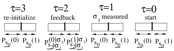
Figure 1: This Szilard engine is modeled by the CB net given by Eq.(59).

Define

$$\Delta H_{vol}=H({\,\underline{s}\,}_{0})-H({\,\underline{s}\,}_{2}|{\,\underline{\sigma}\,}_{1})\;.$$ (60)

The work done by the system when it changes its volume from $V_{0}$ at time $\tau=0$ to $V_{2}$ at time $\tau=2$ is

$${\cancel{\Delta}}W_{vol}=\int_{V_{0}}^{V_{2}}dV\;P=\int_{V_{0}}^{V_{2}}dV\;\frac{T}{V}=T\ln\frac{V_{2}}{V_{0}}=T\left\langle\ln\frac{P(s_{2}|\sigma_{1})}{P(s_{0})}\right\rangle=T\Delta H_{vol}\;.$$ (61)

(We assume an ideal gas so $PV=Nk_{B}T$ but $N=1$ and we are setting $k_{B}=1$ so $PV=T$)

The following table is easy to verify using standard identities in Shannon Information Theory (specially the chain rule identities).

$$\begin{array}[]{l|l|l|}&\hbox{ system }{\,\underline{s}}&\hbox{ system }{\,\underline{s}\,}+\hbox{ sensor }{\,\underline{\sigma}}\\ \hline\cr 1\leftarrow 0&H({\,\underline{s}\,}_{\tau}){|_{\tau=0}^{1}}=&H({\,\underline{s}\,}_{\tau},{\,\underline{\sigma}\,}_{\tau}){|_{\tau=0}^{1}}=\\ &=0&=-H({\,\underline{\sigma}\,}_{1}:{\,\underline{s}\,}_{0})+H({\,\underline{\sigma}\,}_{1})\\ \hline\cr 2\leftarrow 1&H({\,\underline{s}\,}_{\tau}){|_{\tau=1}^{2}}=&H({\,\underline{s}\,}_{\tau},{\,\underline{\sigma}\,}_{\tau}){|_{\tau=1}^{2}}=\\ &=-\Delta H_{vol}+H({\,\underline{s}\,}_{2}:{\,\underline{\sigma}\,}_{1})&=-\Delta H_{vol}+H({\,\underline{\sigma}\,}_{1}:{\,\underline{s}\,}_{0})\\ \hline\cr 3\leftarrow 2&H({\,\underline{s}\,}_{\tau}){|_{\tau=2}^{3}}=&H({\,\underline{s}\,}_{\tau},{\,\underline{\sigma}\,}_{\tau}){|_{\tau=2}^{3}}=\\ &=\Delta H_{vol}-H({\,\underline{s}\,}_{2}:{\,\underline{\sigma}\,}_{1})&=\Delta H_{vol}-H({\,\underline{\sigma}\,}_{1})\\ \hline\cr 0\leftarrow 3&H({\,\underline{s}\,}_{\tau}){|_{\tau=3}^{0}}=&H({\,\underline{s}\,}_{\tau},{\,\underline{\sigma}\,}_{\tau}){|_{\tau=3}^{0}}=\\ &=0&=0\\ \hline\cr\end{array}\;$$ (62)

The entropy change over a full cycle is zero, as expected. For some of the $\tau$, the entropy change $H({\,\underline{s}\,}_{\tau},\sigma_{\tau}){|_{\tau=0}^{\tau}}$ contains “Landauer erasure-work terms” $TH(\sigma_{1})$, “Maxwell volume-work terms” $T\Delta H_{vol}$, and even “correlation-energy terms” $TH({\,\underline{\sigma}\,}_{1}:{\,\underline{s}\,}_{0})$ (these measure a sort of internal energy), but they all manage to cancel each other out over a full cycle.

5.2 Q1 Case

In this case, we will abbreviate $\rho_{\tau}=\rho_{\tau;{\,\underline{s}\,}_{\tau},{\,\underline{\sigma}\,}_{\tau}}$ and $S_{\tau}(\cdot)=S_{\rho_{\tau}}(\cdot)$. Also, in this case, $X=(s,\sigma)$.

We begin by specifying the form of $\rho_{\tau}$ that we will assume for $\tau=0,1,2,3$.

We will assume that the sensor random variable ${\,\underline{\sigma}\,}_{\tau}$ is a classical random variable for all $\tau$. Hence, ${\,\underline{\sigma}\,}_{\tau}=({\,\underline{\sigma}\,}_{\tau})_{cl}$ for all $\tau$.

• At time $\tau=0$,

  $$\rho_{0}=\sum_{r_{0}}\sum_{\sigma_{0}}{\left[\begin{array}[]{c}\sum_{s_{0}}|X_{0}\rangle A(X_{0},r_{0})\end{array}\right]}{\left[\begin{array}[]{c}{\rm h.c.}\end{array}\right]}\;,$$ (63)

  where

  $$A(X_{0},r_{0})=A(s_{0},r_{0})\delta(\sigma_{0},0)\;,$$ (64)

  and

  $$\sum_{s_{0},r_{0}}|A(s_{0},r_{0})|^{2}=1\;.$$ (65)

  $\rho_{0}$ can be represented as a QB net as follows:

  $$\rho_{0}=\begin{array}[]{l}{\rm cl}_{{\,\underline{\sigma}\,}_{0}}\\ {\rm tr}_{{\,\underline{r}\,}_{0}}\end{array}{\left[\begin{array}[]{c}\ignorespaces\lx@xy@svg{\hbox{\raise 0.0pt\hbox{\kern 11.56664pt\hbox{\ignorespaces\ignorespaces\ignorespaces\hbox{\vtop{\kern 0.0pt\offinterlineskip\halign{\entry@#!@&&\entry@@#!@\cr&\\&\crcr}}}\ignorespaces{{{\hbox{\ellipsed@{11.56662pt}{9.74109pt}}}}\hbox{\kern-11.56664pt\raise 0.0pt\hbox{\hbox{\kern 6.0pt\raise-1.93666pt\hbox{$\textstyle{{\,\underline{s}\,}_{0}\ignorespaces\ignorespaces\ignorespaces\ignorespaces}$}}}}}\ignorespaces\ignorespaces\ignorespaces{}{}\ignorespaces{}{\hbox{\lx@xy@droprule}}\ignorespaces{\hbox{\kern 17.56664pt\raise 0.0pt\hbox{\hbox{\kern 0.0pt\raise 0.0pt\hbox{\lx@xy@tip{1}\lx@xy@tip{-1}}}}}}{\hbox{\lx@xy@droprule}}{\hbox{\lx@xy@droprule}}{{{\hbox{\ellipsed@{11.56662pt}{9.74109pt}}}}\hbox{\kern 17.56664pt\raise 0.0pt\hbox{\hbox{\kern 6.0pt\raise-1.93666pt\hbox{$\textstyle{{\,\underline{r}\,}_{0}}$}}}}}{{{\hbox{\ellipsed@{11.56662pt}{9.74109pt}}}}\hbox{\kern-11.56664pt\raise-25.48221pt\hbox{\hbox{\kern 6.0pt\raise-1.93666pt\hbox{$\textstyle{{\,\underline{\sigma}\,}_{0}}$}}}}}{\hbox{\kern 29.13327pt\raise-25.48221pt\hbox{\hbox{\kern 0.0pt\raise 0.0pt\hbox{$\textstyle{}$}}}}}\ignorespaces\ignorespaces\ignorespaces{}\ignorespaces{}\ignorespaces\ignorespaces\ignorespaces{\hbox{\kern 9.81664pt\raise-30.73776pt\hbox{{}\hbox{\kern 0.0pt\raise 0.0pt\hbox{\hbox{\kern 3.0pt\hbox{\hbox{\kern 0.0pt\raise-2.25555pt\hbox{$\scriptstyle{0}$}}}\kern 3.0pt}}}}}}\ignorespaces{}\ignorespaces}}}}\ignorespaces\end{array}\right]}{\left[\begin{array}[]{c}{\rm h.c.}\end{array}\right]}\;. \textstyle{{\,\underline{s}\,}_{0}\ignorespaces\ignorespaces\ignorespaces\ignorespaces} \textstyle{{\,\underline{r}\,}_{0}} \textstyle{{\,\underline{\sigma}\,}_{0}} \scriptstyle{0} \textstyle{{\,\underline{s}\,}_{0}\ignorespaces\ignorespaces\ignorespaces\ignorespaces} \textstyle{{\,\underline{r}\,}_{0}} \textstyle{{\,\underline{\sigma}\,}_{0}} \scriptstyle{0}$$ (66)

• At time $\tau=1$,

  $$\rho_{1}=\sum_{r_{0}}\sum_{\sigma_{1\;:\;0}}{\left[\begin{array}[]{c}\sum_{s_{1\;:\;0}}\begin{array}[]{r}|X_{1}\rangle A(X_{1}|X_{0})\\ A(X_{0},r_{0})\end{array}\end{array}\right]}{\left[\begin{array}[]{c}{\rm h.c.}\end{array}\right]}\;,$$ (67)

  where $A(X_{1}|X_{0})$ is an isometry.

  $\rho_{1}$ can be represented as a QB net as follows:

  $$\rho_{1}=\begin{array}[]{l}{\rm cl}_{{\,\underline{\sigma}\,}_{1}}\\ {\rm tr}_{{\,\underline{\sigma}\,}_{0}}\\ {\rm tr}_{{\,\underline{r}\,}_{0}}\end{array}{\left[\begin{array}[]{c}\ignorespaces\lx@xy@svg{\hbox{\raise 0.0pt\hbox{\kern 11.56664pt\hbox{\ignorespaces\ignorespaces\ignorespaces\hbox{\vtop{\kern 0.0pt\offinterlineskip\halign{\entry@#!@&&\entry@@#!@\cr&&&\\&&&\\&&&\crcr}}}\ignorespaces{{{\hbox{\ellipsed@{11.56662pt}{9.74109pt}}}}\hbox{\kern-11.56664pt\raise 0.0pt\hbox{\hbox{\kern 6.0pt\raise-1.93666pt\hbox{$\textstyle{{\,\underline{s}\,}_{1}}$}}}}}{\hbox{\kern 34.87212pt\raise 0.0pt\hbox{\hbox{\kern 0.0pt\raise 0.0pt\hbox{$\textstyle{}$}}}}}{{{\hbox{\ellipsed@{11.56662pt}{9.74109pt}}}}\hbox{\kern 58.1776pt\raise 0.0pt\hbox{\hbox{\kern 6.0pt\raise-1.93666pt\hbox{$\textstyle{\cancel{{\,\underline{s}\,}_{0}}\ignorespaces\ignorespaces\ignorespaces\ignorespaces\ignorespaces\ignorespaces\ignorespaces\ignorespaces}$}}}}}\ignorespaces\ignorespaces{{{}{}{}{}}}{}\ignorespaces{}{{}}\ignorespaces{{}}{{{{}{}{}{}}}}\ignorespaces{\hbox{\lx@xy@drawline@}}\ignorespaces{\hbox{\kern 46.17755pt\raise-15.0401pt\hbox{\hbox{\kern 0.0pt\raise 0.0pt\hbox{\lx@xy@tip{1}\lx@xy@tip{-1}}}}}}{{}}\ignorespaces{{{{}{}{}{}}}}\ignorespaces{\hbox{\lx@xy@drawline@}}{{}}\ignorespaces{{{}{}{}{}}}{\hbox{\lx@xy@drawline@}}\ignorespaces\ignorespaces\ignorespaces{}{}\ignorespaces{}{\hbox{\lx@xy@droprule}}\ignorespaces{\hbox{\kern 87.31087pt\raise 0.0pt\hbox{\hbox{\kern 0.0pt\raise 0.0pt\hbox{\lx@xy@tip{1}\lx@xy@tip{-1}}}}}}{\hbox{\lx@xy@droprule}}{\hbox{\lx@xy@droprule}}{{{\hbox{\ellipsed@{11.56662pt}{9.74109pt}}}}\hbox{\kern 87.31087pt\raise 0.0pt\hbox{\hbox{\kern 6.0pt\raise-1.93666pt\hbox{$\textstyle{{\,\underline{r}\,}_{0}}$}}}}}{\hbox{\kern 0.0pt\raise-22.26053pt\hbox{\hbox{\kern 0.0pt\raise 0.0pt\hbox{$\textstyle{}$}}}}}{{{\hbox{\ellipsed@{17.30548pt}{9.51942pt}}}}\hbox{\kern 17.56664pt\raise-22.26053pt\hbox{\hbox{\kern 6.0pt\raise-2.15834pt\hbox{$\textstyle{\scriptstyle\cancel{{\,\underline{s}\,}_{1},{\,\underline{\sigma}\,}_{1}}\ignorespaces\ignorespaces\ignorespaces\ignorespaces\ignorespaces\ignorespaces\ignorespaces\ignorespaces}$}}}}}\ignorespaces\ignorespaces{}{{{}{}{}{}}}\ignorespaces{}{{{{}{}{}{}}}}\ignorespaces{{{{}{}{}{}}}}{{}}\ignorespaces{\hbox{\lx@xy@drawline@}}\ignorespaces\ignorespaces\ignorespaces{\hbox{\kern 10.0966pt\raise-2.06984pt\hbox{{}\hbox{\kern 0.0pt\raise 0.0pt\hbox{\hbox{\kern 3.0pt\hbox{\hbox{\kern 0.0pt\raise-2.43056pt\hbox{$\scriptstyle{\delta}$}}}\kern 3.0pt}}}}}}\ignorespaces{\hbox{\kern 9.21432pt\raise-5.88564pt\hbox{\hbox{\kern 0.0pt\raise 0.0pt\hbox{\lx@xy@tip{1}\lx@xy@tip{-1}}}}}}{{{{}{}{}{}}}}\ignorespaces{{}}\ignorespaces{\hbox{\lx@xy@drawline@}}{{{{}{}{}{}}}}\ignorespaces{}{\hbox{\lx@xy@drawline@}}\ignorespaces\ignorespaces{}{{{}{}{}{}}}\ignorespaces{}{{{{}{}{}{}}}}\ignorespaces{{{{}{}{}{}}}}{{}}\ignorespaces\ignorespaces\ignorespaces\ignorespaces{\hbox{\kern 4.2776pt\raise-31.5901pt\hbox{{}\hbox{\kern 0.0pt\raise 0.0pt\hbox{\hbox{\kern 3.0pt\hbox{\hbox{\kern 0.0pt\raise-2.43056pt\hbox{$\scriptstyle{\delta}$}}}\kern 3.0pt}}}}}}\ignorespaces{\hbox{\kern 9.21432pt\raise-38.63542pt\hbox{\hbox{\kern 0.0pt\raise 0.0pt\hbox{\lx@xy@tip{1}\lx@xy@tip{-1}}}}}}{{{{}{}{}{}}}}\ignorespaces{{}}\ignorespaces{\hbox{\lx@xy@drawline@}}{{{{}{}{}{}}}}\ignorespaces{}{\hbox{\lx@xy@drawline@}}{\hbox{\kern 69.74423pt\raise-22.26053pt\hbox{\hbox{\kern 0.0pt\raise 0.0pt\hbox{$\textstyle{}$}}}}}{\hbox{\kern 98.8775pt\raise-22.26053pt\hbox{\hbox{\kern 0.0pt\raise 0.0pt\hbox{$\textstyle{}$}}}}}{{{\hbox{\ellipsed@{11.56662pt}{9.74109pt}}}}\hbox{\kern-11.56664pt\raise-44.52106pt\hbox{\hbox{\kern 6.0pt\raise-1.93666pt\hbox{$\textstyle{{\,\underline{\sigma}\,}_{1}}$}}}}}{\hbox{\kern 34.87212pt\raise-44.52106pt\hbox{\hbox{\kern 0.0pt\raise 0.0pt\hbox{$\textstyle{}$}}}}}{{{\hbox{\ellipsed@{11.56662pt}{9.74109pt}}}}\hbox{\kern 58.1776pt\raise-44.52106pt\hbox{\hbox{\kern 6.0pt\raise-1.93666pt\hbox{$\textstyle{{\,\underline{\sigma}\,}_{0}\ignorespaces\ignorespaces\ignorespaces\ignorespaces}$}}}}}\ignorespaces\ignorespaces{{{}{}{}{}}}{}\ignorespaces{}{{}}\ignorespaces{{}}{{{{}{}{}{}}}}\ignorespaces{\hbox{\lx@xy@drawline@}}\ignorespaces{\hbox{\kern 46.17755pt\raise-29.48096pt\hbox{\hbox{\kern 0.0pt\raise 0.0pt\hbox{\lx@xy@tip{1}\lx@xy@tip{-1}}}}}}{{}}\ignorespaces{{{{}{}{}{}}}}\ignorespaces{\hbox{\lx@xy@drawline@}}{{}}\ignorespaces{{{}{}{}{}}}{\hbox{\lx@xy@drawline@}}{\hbox{\kern 98.8775pt\raise-44.52106pt\hbox{\hbox{\kern 0.0pt\raise 0.0pt\hbox{$\textstyle{}$}}}}}\ignorespaces\ignorespaces\ignorespaces{}\ignorespaces{}\ignorespaces\ignorespaces\ignorespaces{\hbox{\kern 79.56087pt\raise-49.77661pt\hbox{{}\hbox{\kern 0.0pt\raise 0.0pt\hbox{\hbox{\kern 3.0pt\hbox{\hbox{\kern 0.0pt\raise-2.25555pt\hbox{$\scriptstyle{0}$}}}\kern 3.0pt}}}}}}\ignorespaces{}\ignorespaces}}}}\ignorespaces\end{array}\right]}{\left[\begin{array}[]{c}{\rm h.c.}\end{array}\right]}\;. \textstyle{{\,\underline{s}\,}_{1}} \textstyle{{\,\underline{r}\,}_{0}} \textstyle{\scriptstyle\cancel{{\,\underline{s}\,}_{1},{\,\underline{\sigma}\,}_{1}}\ignorespaces\ignorespaces\ignorespaces\ignorespaces\ignorespaces\ignorespaces\ignorespaces\ignorespaces} \scriptstyle{\delta} \scriptstyle{\delta} \textstyle{{\,\underline{\sigma}\,}_{1}} \textstyle{{\,\underline{\sigma}\,}_{0}\ignorespaces\ignorespaces\ignorespaces\ignorespaces} \scriptstyle{0} \textstyle{{\,\underline{s}\,}_{1}} \textstyle{{\,\underline{r}\,}_{0}} \textstyle{\scriptstyle\cancel{{\,\underline{s}\,}_{1},{\,\underline{\sigma}\,}_{1}}\ignorespaces\ignorespaces\ignorespaces\ignorespaces\ignorespaces\ignorespaces\ignorespaces\ignorespaces} \scriptstyle{\delta} \scriptstyle{\delta} \textstyle{{\,\underline{\sigma}\,}_{1}} \textstyle{{\,\underline{\sigma}\,}_{0}\ignorespaces\ignorespaces\ignorespaces\ignorespaces} \scriptstyle{0}$$ (68)

• At time $\tau=2$,

  $$\rho_{2}=\sum_{r_{0}}\sum_{\sigma_{2\;:\;0}}{\left[\begin{array}[]{c}\sum_{s_{2\;:\;0}}\begin{array}[]{r}|X_{2}\rangle A(X_{2}|X_{1})\\ A(X_{1}|X_{0})\\ A(X_{0},r_{0})\end{array}\end{array}\right]}{\left[\begin{array}[]{c}{\rm h.c.}\end{array}\right]}\;,$$ (69)

  where

  $$A(X_{2}|X_{1})=A(s_{2}|s_{1},\sigma_{1})\delta(\sigma_{2},\sigma_{1})\;$$ (70)

  and, for all $\sigma_{1}$,

  $$\sum_{s_{2}}{\left[\begin{array}[]{c}A(s_{2}|s_{1},\sigma_{1})\end{array}\right]}{\left[\begin{array}[]{c}{\rm h.c.}\\ s_{1}\rightarrow s_{1}^{\prime}\end{array}\right]}=\delta(s_{1},s_{1}^{\prime})\;.$$ (71)

  $\rho_{2}$ can be represented as a QB net as follows:

  $$\rho_{2}=\begin{array}[]{l}{\rm cl}_{{\,\underline{\sigma}\,}_{2}}\\ {\rm tr}_{{\,\underline{\sigma}\,}_{1\;:\;0}}\\ {\rm tr}_{{\,\underline{r}\,}_{0}}\end{array}{\left[\begin{array}[]{c}\ignorespaces\lx@xy@svg{\hbox{\raise 0.0pt\hbox{\kern 11.56664pt\hbox{\ignorespaces\ignorespaces\ignorespaces\hbox{\vtop{\kern 0.0pt\offinterlineskip\halign{\entry@#!@&&\entry@@#!@\cr&&&&&\\&&&&&\\&&&&&\crcr}}}\ignorespaces{{{\hbox{\ellipsed@{11.56662pt}{9.74109pt}}}}\hbox{\kern-11.56664pt\raise 0.0pt\hbox{\hbox{\kern 6.0pt\raise-1.93666pt\hbox{$\textstyle{{\,\underline{s}\,}_{2}}$}}}}}{\hbox{\kern 34.87212pt\raise 0.0pt\hbox{\hbox{\kern 0.0pt\raise 0.0pt\hbox{$\textstyle{}$}}}}}{{{\hbox{\ellipsed@{11.56662pt}{9.74109pt}}}}\hbox{\kern 58.1776pt\raise 0.0pt\hbox{\hbox{\kern 6.0pt\raise-1.93666pt\hbox{$\textstyle{\cancel{{\,\underline{s}\,}_{1}}\ignorespaces\ignorespaces\ignorespaces\ignorespaces}$}}}}}\ignorespaces\ignorespaces{{{}{}{}{}}}{}\ignorespaces{}{{}}\ignorespaces{{}}{{{{}{}{}{}}}}\ignorespaces{\hbox{\lx@xy@drawline@}}\ignorespaces{\hbox{\kern 46.17755pt\raise-15.0401pt\hbox{\hbox{\kern 0.0pt\raise 0.0pt\hbox{\lx@xy@tip{1}\lx@xy@tip{-1}}}}}}{{}}\ignorespaces{{{{}{}{}{}}}}\ignorespaces{\hbox{\lx@xy@drawline@}}{{}}\ignorespaces{{{}{}{}{}}}{\hbox{\lx@xy@drawline@}}{\hbox{\kern 104.61635pt\raise 0.0pt\hbox{\hbox{\kern 0.0pt\raise 0.0pt\hbox{$\textstyle{}$}}}}}{{{\hbox{\ellipsed@{11.56662pt}{9.74109pt}}}}\hbox{\kern 127.92183pt\raise 0.0pt\hbox{\hbox{\kern 6.0pt\raise-1.93666pt\hbox{$\textstyle{\cancel{{\,\underline{s}\,}_{0}}\ignorespaces\ignorespaces\ignorespaces\ignorespaces\ignorespaces\ignorespaces\ignorespaces\ignorespaces}$}}}}}\ignorespaces\ignorespaces{{{}{}{}{}}}{}\ignorespaces{}{{}}\ignorespaces{{}}{{{{}{}{}{}}}}\ignorespaces{\hbox{\lx@xy@drawline@}}\ignorespaces{\hbox{\kern 115.92178pt\raise-15.0401pt\hbox{\hbox{\kern 0.0pt\raise 0.0pt\hbox{\lx@xy@tip{1}\lx@xy@tip{-1}}}}}}{{}}\ignorespaces{{{{}{}{}{}}}}\ignorespaces{\hbox{\lx@xy@drawline@}}{{}}\ignorespaces{{{}{}{}{}}}{\hbox{\lx@xy@drawline@}}\ignorespaces\ignorespaces\ignorespaces{}{}\ignorespaces{}{\hbox{\lx@xy@droprule}}\ignorespaces{\hbox{\kern 157.0551pt\raise 0.0pt\hbox{\hbox{\kern 0.0pt\raise 0.0pt\hbox{\lx@xy@tip{1}\lx@xy@tip{-1}}}}}}{\hbox{\lx@xy@droprule}}{\hbox{\lx@xy@droprule}}{{{\hbox{\ellipsed@{11.56662pt}{9.74109pt}}}}\hbox{\kern 157.0551pt\raise 0.0pt\hbox{\hbox{\kern 6.0pt\raise-1.93666pt\hbox{$\textstyle{{\,\underline{r}\,}_{0}}$}}}}}{\hbox{\kern 0.0pt\raise-22.26053pt\hbox{\hbox{\kern 0.0pt\raise 0.0pt\hbox{$\textstyle{}$}}}}}{{{\hbox{\ellipsed@{17.30548pt}{9.51942pt}}}}\hbox{\kern 17.56664pt\raise-22.26053pt\hbox{\hbox{\kern 6.0pt\raise-2.15834pt\hbox{$\textstyle{\scriptstyle\cancel{{\,\underline{s}\,}_{2},{\,\underline{\sigma}\,}_{2}}\ignorespaces\ignorespaces\ignorespaces\ignorespaces\ignorespaces\ignorespaces\ignorespaces\ignorespaces}$}}}}}\ignorespaces\ignorespaces{}{{{}{}{}{}}}\ignorespaces{}{{{{}{}{}{}}}}\ignorespaces{{{{}{}{}{}}}}{{}}\ignorespaces{\hbox{\lx@xy@drawline@}}\ignorespaces\ignorespaces\ignorespaces{\hbox{\kern 10.0966pt\raise-2.06984pt\hbox{{}\hbox{\kern 0.0pt\raise 0.0pt\hbox{\hbox{\kern 3.0pt\hbox{\hbox{\kern 0.0pt\raise-2.43056pt\hbox{$\scriptstyle{\delta}$}}}\kern 3.0pt}}}}}}\ignorespaces{\hbox{\kern 9.21432pt\raise-5.88564pt\hbox{\hbox{\kern 0.0pt\raise 0.0pt\hbox{\lx@xy@tip{1}\lx@xy@tip{-1}}}}}}{{{{}{}{}{}}}}\ignorespaces{{}}\ignorespaces{\hbox{\lx@xy@drawline@}}{{{{}{}{}{}}}}\ignorespaces{}{\hbox{\lx@xy@drawline@}}\ignorespaces\ignorespaces{}{{{}{}{}{}}}\ignorespaces{}{{{{}{}{}{}}}}\ignorespaces{{{{}{}{}{}}}}{{}}\ignorespaces\ignorespaces\ignorespaces\ignorespaces{\hbox{\kern 4.2776pt\raise-31.5901pt\hbox{{}\hbox{\kern 0.0pt\raise 0.0pt\hbox{\hbox{\kern 3.0pt\hbox{\hbox{\kern 0.0pt\raise-2.43056pt\hbox{$\scriptstyle{\delta}$}}}\kern 3.0pt}}}}}}\ignorespaces{\hbox{\kern 9.21432pt\raise-38.63542pt\hbox{\hbox{\kern 0.0pt\raise 0.0pt\hbox{\lx@xy@tip{1}\lx@xy@tip{-1}}}}}}{{{{}{}{}{}}}}\ignorespaces{{}}\ignorespaces{\hbox{\lx@xy@drawline@}}{{{{}{}{}{}}}}\ignorespaces{}{\hbox{\lx@xy@drawline@}}{\hbox{\kern 69.74423pt\raise-22.26053pt\hbox{\hbox{\kern 0.0pt\raise 0.0pt\hbox{$\textstyle{}$}}}}}{{{\hbox{\ellipsed@{17.30548pt}{9.51942pt}}}}\hbox{\kern 87.31087pt\raise-22.26053pt\hbox{\hbox{\kern 6.0pt\raise-2.15834pt\hbox{$\textstyle{\scriptstyle\cancel{{\,\underline{s}\,}_{1},{\,\underline{\sigma}\,}_{1}}\ignorespaces\ignorespaces\ignorespaces\ignorespaces\ignorespaces\ignorespaces\ignorespaces\ignorespaces}$}}}}}\ignorespaces\ignorespaces{}{{{}{}{}{}}}\ignorespaces{}{{{{}{}{}{}}}}\ignorespaces{{{{}{}{}{}}}}{{}}\ignorespaces{\hbox{\lx@xy@drawline@}}\ignorespaces\ignorespaces\ignorespaces{\hbox{\kern 79.84084pt\raise-2.06984pt\hbox{{}\hbox{\kern 0.0pt\raise 0.0pt\hbox{\hbox{\kern 3.0pt\hbox{\hbox{\kern 0.0pt\raise-2.43056pt\hbox{$\scriptstyle{\delta}$}}}\kern 3.0pt}}}}}}\ignorespaces{\hbox{\kern 78.95856pt\raise-5.88564pt\hbox{\hbox{\kern 0.0pt\raise 0.0pt\hbox{\lx@xy@tip{1}\lx@xy@tip{-1}}}}}}{{{{}{}{}{}}}}\ignorespaces{{}}\ignorespaces{\hbox{\lx@xy@drawline@}}{{{{}{}{}{}}}}\ignorespaces{}{\hbox{\lx@xy@drawline@}}\ignorespaces\ignorespaces{}{{{}{}{}{}}}\ignorespaces{}{{{{}{}{}{}}}}\ignorespaces{{{{}{}{}{}}}}{{}}\ignorespaces\ignorespaces\ignorespaces\ignorespaces{\hbox{\kern 74.02184pt\raise-31.5901pt\hbox{{}\hbox{\kern 0.0pt\raise 0.0pt\hbox{\hbox{\kern 3.0pt\hbox{\hbox{\kern 0.0pt\raise-2.43056pt\hbox{$\scriptstyle{\delta}$}}}\kern 3.0pt}}}}}}\ignorespaces{\hbox{\kern 78.95856pt\raise-38.63542pt\hbox{\hbox{\kern 0.0pt\raise 0.0pt\hbox{\lx@xy@tip{1}\lx@xy@tip{-1}}}}}}{{{{}{}{}{}}}}\ignorespaces{{}}\ignorespaces{\hbox{\lx@xy@drawline@}}{{{{}{}{}{}}}}\ignorespaces{}{\hbox{\lx@xy@drawline@}}{\hbox{\kern 139.48846pt\raise-22.26053pt\hbox{\hbox{\kern 0.0pt\raise 0.0pt\hbox{$\textstyle{}$}}}}}{\hbox{\kern 168.62173pt\raise-22.26053pt\hbox{\hbox{\kern 0.0pt\raise 0.0pt\hbox{$\textstyle{}$}}}}}{{{\hbox{\ellipsed@{11.56662pt}{9.74109pt}}}}\hbox{\kern-11.56664pt\raise-44.52106pt\hbox{\hbox{\kern 6.0pt\raise-1.93666pt\hbox{$\textstyle{{\,\underline{\sigma}\,}_{2}}$}}}}}{\hbox{\kern 34.87212pt\raise-44.52106pt\hbox{\hbox{\kern 0.0pt\raise 0.0pt\hbox{$\textstyle{}$}}}}}{{{\hbox{\ellipsed@{11.56662pt}{9.74109pt}}}}\hbox{\kern 58.1776pt\raise-44.52106pt\hbox{\hbox{\kern 6.0pt\raise-1.93666pt\hbox{$\textstyle{{\,\underline{\sigma}\,}_{1}\ignorespaces\ignorespaces\ignorespaces\ignorespaces}$}}}}}\ignorespaces\ignorespaces{{{}{}{}{}}}{}\ignorespaces{}{{}}\ignorespaces{{}}{{{{}{}{}{}}}}\ignorespaces{\hbox{\lx@xy@drawline@}}\ignorespaces{\hbox{\kern 46.17755pt\raise-29.48096pt\hbox{\hbox{\kern 0.0pt\raise 0.0pt\hbox{\lx@xy@tip{1}\lx@xy@tip{-1}}}}}}{{}}\ignorespaces{{{{}{}{}{}}}}\ignorespaces{\hbox{\lx@xy@drawline@}}{{}}\ignorespaces{{{}{}{}{}}}{\hbox{\lx@xy@drawline@}}{\hbox{\kern 104.61635pt\raise-44.52106pt\hbox{\hbox{\kern 0.0pt\raise 0.0pt\hbox{$\textstyle{}$}}}}}{{{\hbox{\ellipsed@{11.56662pt}{9.74109pt}}}}\hbox{\kern 127.92183pt\raise-44.52106pt\hbox{\hbox{\kern 6.0pt\raise-1.93666pt\hbox{$\textstyle{{\,\underline{\sigma}\,}_{0}\ignorespaces\ignorespaces\ignorespaces\ignorespaces}$}}}}}\ignorespaces\ignorespaces{{{}{}{}{}}}{}\ignorespaces{}{{}}\ignorespaces{{}}{{{{}{}{}{}}}}\ignorespaces{\hbox{\lx@xy@drawline@}}\ignorespaces{\hbox{\kern 115.92178pt\raise-29.48096pt\hbox{\hbox{\kern 0.0pt\raise 0.0pt\hbox{\lx@xy@tip{1}\lx@xy@tip{-1}}}}}}{{}}\ignorespaces{{{{}{}{}{}}}}\ignorespaces{\hbox{\lx@xy@drawline@}}{{}}\ignorespaces{{{}{}{}{}}}{\hbox{\lx@xy@drawline@}}{\hbox{\kern 168.62173pt\raise-44.52106pt\hbox{\hbox{\kern 0.0pt\raise 0.0pt\hbox{$\textstyle{}$}}}}}\ignorespaces\ignorespaces\ignorespaces{}\ignorespaces{}\ignorespaces\ignorespaces\ignorespaces{\hbox{\kern 149.3051pt\raise-49.77661pt\hbox{{}\hbox{\kern 0.0pt\raise 0.0pt\hbox{\hbox{\kern 3.0pt\hbox{\hbox{\kern 0.0pt\raise-2.25555pt\hbox{$\scriptstyle{0}$}}}\kern 3.0pt}}}}}}\ignorespaces{}\ignorespaces}}}}\ignorespaces\end{array}\right]}{\left[\begin{array}[]{c}{\rm h.c.}\end{array}\right]}\;. \textstyle{{\,\underline{s}\,}_{2}} \textstyle{{\,\underline{r}\,}_{0}} \textstyle{\scriptstyle\cancel{{\,\underline{s}\,}_{2},{\,\underline{\sigma}\,}_{2}}\ignorespaces\ignorespaces\ignorespaces\ignorespaces\ignorespaces\ignorespaces\ignorespaces\ignorespaces} \scriptstyle{\delta} \scriptstyle{\delta} \textstyle{\scriptstyle\cancel{{\,\underline{s}\,}_{1},{\,\underline{\sigma}\,}_{1}}\ignorespaces\ignorespaces\ignorespaces\ignorespaces\ignorespaces\ignorespaces\ignorespaces\ignorespaces} \scriptstyle{\delta} \scriptstyle{\delta} \textstyle{{\,\underline{\sigma}\,}_{2}} \textstyle{{\,\underline{\sigma}\,}_{1}\ignorespaces\ignorespaces\ignorespaces\ignorespaces} \textstyle{{\,\underline{\sigma}\,}_{0}\ignorespaces\ignorespaces\ignorespaces\ignorespaces} \scriptstyle{0} \textstyle{{\,\underline{s}\,}_{2}} \textstyle{{\,\underline{r}\,}_{0}} \textstyle{\scriptstyle\cancel{{\,\underline{s}\,}_{2},{\,\underline{\sigma}\,}_{2}}\ignorespaces\ignorespaces\ignorespaces\ignorespaces\ignorespaces\ignorespaces\ignorespaces\ignorespaces} \scriptstyle{\delta} \scriptstyle{\delta} \textstyle{\scriptstyle\cancel{{\,\underline{s}\,}_{1},{\,\underline{\sigma}\,}_{1}}\ignorespaces\ignorespaces\ignorespaces\ignorespaces\ignorespaces\ignorespaces\ignorespaces\ignorespaces} \scriptstyle{\delta} \scriptstyle{\delta} \textstyle{{\,\underline{\sigma}\,}_{2}} \textstyle{{\,\underline{\sigma}\,}_{1}\ignorespaces\ignorespaces\ignorespaces\ignorespaces} \textstyle{{\,\underline{\sigma}\,}_{0}\ignorespaces\ignorespaces\ignorespaces\ignorespaces} \scriptstyle{0}$$ (72)

• At time $\tau=3$,

  $$\rho_{3}=\sum_{R_{3},r_{3}}\sum_{r_{0}}\sum_{\sigma_{3\;:\;0}}{\left[\begin{array}[]{c}\sum_{s_{3\;:\;0}}\begin{array}[]{r}|X_{3}\rangle A(X_{3},R_{3},r_{3}|X_{2})\\ A(X_{2}|X_{1})\\ A(X_{1}|X_{0})\\ A(X_{0},r_{0})\end{array}\end{array}\right]}{\left[\begin{array}[]{c}{\rm h.c.}\end{array}\right]}\;,$$ (73)

  where

  $$A(X_{3},R_{3},r_{3}|X_{2})=A_{{\,\underline{s}\,}_{0},{\,\underline{r}\,}_{0}}(s_{3},r_{3})\delta(\sigma_{3},0)A(R_{3}|s_{2},\sigma_{2})\;$$ (74)

  and $A(R_{3}|s_{2},\sigma_{2})$ is an isometry. Performing the sum over $R_{3}$, Eq.(73) reduces to

  $$\rho_{3}=\sum_{r_{3}}\sum_{\sigma_{3}}{\left[\begin{array}[]{c}\sum_{s_{3}}|X_{3}\rangle A_{{\,\underline{X}\,}_{0},{\,\underline{r}\,}_{0}}(X_{3},r_{3})\end{array}\right]}{\left[\begin{array}[]{c}{\rm h.c.}\end{array}\right]}\;.$$ (75)

  $\rho_{3}$ can be represented as a QB net as follows:

  $$\rho_{3}=\begin{array}[]{l}{\rm cl}_{{\,\underline{\sigma}\,}_{3}}\\ {\rm tr}_{{\,\underline{r}\,}_{3}}\end{array}{\left[\begin{array}[]{c}\ignorespaces\lx@xy@svg{\hbox{\raise 0.0pt\hbox{\kern 11.56664pt\hbox{\ignorespaces\ignorespaces\ignorespaces\hbox{\vtop{\kern 0.0pt\offinterlineskip\halign{\entry@#!@&&\entry@@#!@\cr&\\&\crcr}}}\ignorespaces{{{\hbox{\ellipsed@{11.56662pt}{9.74109pt}}}}\hbox{\kern-11.56664pt\raise 0.0pt\hbox{\hbox{\kern 6.0pt\raise-1.93666pt\hbox{$\textstyle{{\,\underline{s}\,}_{3}\ignorespaces\ignorespaces\ignorespaces\ignorespaces}$}}}}}\ignorespaces\ignorespaces\ignorespaces{}{}\ignorespaces{}{\hbox{\lx@xy@droprule}}\ignorespaces{\hbox{\kern 17.56664pt\raise 0.0pt\hbox{\hbox{\kern 0.0pt\raise 0.0pt\hbox{\lx@xy@tip{1}\lx@xy@tip{-1}}}}}}{\hbox{\lx@xy@droprule}}{\hbox{\lx@xy@droprule}}{{{\hbox{\ellipsed@{11.56662pt}{9.74109pt}}}}\hbox{\kern 17.56664pt\raise 0.0pt\hbox{\hbox{\kern 6.0pt\raise-1.93666pt\hbox{$\textstyle{{\,\underline{r}\,}_{3}}$}}}}}{{{\hbox{\ellipsed@{11.56662pt}{9.74109pt}}}}\hbox{\kern-11.56664pt\raise-25.48221pt\hbox{\hbox{\kern 6.0pt\raise-1.93666pt\hbox{$\textstyle{{\,\underline{\sigma}\,}_{3}}$}}}}}{\hbox{\kern 29.13327pt\raise-25.48221pt\hbox{\hbox{\kern 0.0pt\raise 0.0pt\hbox{$\textstyle{}$}}}}}\ignorespaces\ignorespaces\ignorespaces{}\ignorespaces{}\ignorespaces\ignorespaces\ignorespaces{\hbox{\kern 9.81664pt\raise-30.73776pt\hbox{{}\hbox{\kern 0.0pt\raise 0.0pt\hbox{\hbox{\kern 3.0pt\hbox{\hbox{\kern 0.0pt\raise-2.25555pt\hbox{$\scriptstyle{0}$}}}\kern 3.0pt}}}}}}\ignorespaces{}\ignorespaces}}}}\ignorespaces\end{array}\right]}{\left[\begin{array}[]{c}{\rm h.c.}\end{array}\right]}\;. \textstyle{{\,\underline{s}\,}_{3}\ignorespaces\ignorespaces\ignorespaces\ignorespaces} \textstyle{{\,\underline{r}\,}_{3}} \textstyle{{\,\underline{\sigma}\,}_{3}} \scriptstyle{0} \textstyle{{\,\underline{s}\,}_{3}\ignorespaces\ignorespaces\ignorespaces\ignorespaces} \textstyle{{\,\underline{r}\,}_{3}} \textstyle{{\,\underline{\sigma}\,}_{3}} \scriptstyle{0}$$ (76)

For $\tau=1,2$, define

$$\Delta S^{(\tau)}_{vol}=S_{0}({\,\underline{s}\,}_{0})-S_{\tau}({\,\underline{s}\,}_{\tau}|{\,\underline{\sigma}\,}_{1})\;$$ (77)

and

$${\cancel{\Delta}}W^{(\tau)}_{vol}=T\Delta S^{(\tau)}_{vol}\;.$$ (78)

The following table is easy to verify using standard identities in Shannon Information Theory (specially the chain rule identities).

$$\begin{array}[]{l|l|l|}&\hbox{ system }{\,\underline{s}}&\hbox{ system }{\,\underline{s}\,}+\hbox{ sensor }{\,\underline{\sigma}}\\ \hline\cr 1\leftarrow 0&S_{\tau}({\,\underline{s}\,}_{\tau}){|_{\tau=0}^{1}}=&S_{\tau}({\,\underline{s}\,}_{\tau},{\,\underline{\sigma}\,}_{\tau}){|_{\tau=0}^{1}}=\\ &=S_{1}({\,\underline{s}\,}_{1})-S_{0}({\,\underline{s}\,}_{0})&=-\Delta S^{(1)}_{vol}+H({\,\underline{\sigma}\,}_{1})\\ \hline\cr 2\leftarrow 1&S_{\tau}({\,\underline{s}\,}_{\tau}){|_{\tau=1}^{2}}=&S_{\tau}({\,\underline{s}\,}_{\tau},{\,\underline{\sigma}\,}_{\tau}){|_{\tau=1}^{2}}=\\ &=-\Delta S^{(2)}_{vol}+S_{2}({\,\underline{s}\,}_{2}:{\,\underline{\sigma}\,}_{1})+S_{0}({\,\underline{s}\,}_{0})+S_{1}({\,\underline{s}\,}_{1})&=-\Delta S^{(2)}_{vol}+\Delta S^{(1)}_{vol}\\ \hline\cr 3\leftarrow 2&S_{\tau}({\,\underline{s}\,}_{\tau}){|_{\tau=2}^{3}}=&S_{\tau}({\,\underline{s}\,}_{\tau},{\,\underline{\sigma}\,}_{\tau}){|_{\tau=2}^{3}}=\\ &=\Delta S^{(2)}_{vol}-S_{2}({\,\underline{s}\,}_{2}:{\,\underline{\sigma}\,}_{1})&=\Delta S^{(2)}_{vol}-H({\,\underline{\sigma}\,}_{1})\\ \hline\cr 0\leftarrow 3&S_{\tau}({\,\underline{s}\,}_{\tau}){|_{\tau=3}^{0}}=&S_{\tau}({\,\underline{s}\,}_{\tau},{\,\underline{\sigma}\,}_{\tau}){|_{\tau=3}^{0}}=\\ &=0&=0\\ \hline\cr\end{array}\;.$$ (79)

5.3 C2 Case

In this case, $x=(s,t)$, and $X=(x,\sigma)$.

Consider the following CB net

$$\ignorespaces\lx@xy@svg{\hbox{\raise 0.0pt\hbox{\kern 19.35547pt\hbox{\ignorespaces\ignorespaces\ignorespaces\hbox{\vtop{\kern 0.0pt\offinterlineskip\halign{\entry@#!@&&\entry@@#!@\cr&&&&\\&&&&\\&&&&\crcr}}}\ignorespaces{{{\hbox{\ellipsed@{19.35547pt}{9.8111pt}}}}\hbox{\kern-19.35547pt\raise 0.0pt\hbox{\hbox{\kern 6.0pt\raise-1.86667pt\hbox{$\textstyle{{\,\underline{s}\,}_{3},{\,\underline{t}\,}_{3}}$}}}}}{{{\hbox{\ellipsed@{11.56662pt}{9.74109pt}}}}\hbox{\kern 43.35547pt\raise 0.0pt\hbox{\hbox{\kern 6.0pt\raise-1.93666pt\hbox{$\textstyle{{\,\underline{s}\,}_{2}}$}}}}}{{{\hbox{\ellipsed@{11.56662pt}{9.74109pt}}}}\hbox{\kern 90.48874pt\raise 0.0pt\hbox{\hbox{\kern 6.0pt\raise-1.93666pt\hbox{$\textstyle{{\,\underline{s}\,}_{1}}$}}}}}{{{\hbox{\ellipsed@{11.56662pt}{9.74109pt}}}}\hbox{\kern 137.62201pt\raise 0.0pt\hbox{\hbox{\kern 6.0pt\raise-1.93666pt\hbox{$\textstyle{{\,\underline{s}\,}_{0}\ignorespaces\ignorespaces\ignorespaces\ignorespaces\ignorespaces\ignorespaces\ignorespaces\ignorespaces}$}}}}}\ignorespaces\ignorespaces{}{}\ignorespaces{}{{}}\ignorespaces{{}}{{}}\ignorespaces{\hbox{\lx@xy@drawline@}}\ignorespaces{\hbox{\kern 106.85492pt\raise-78.17542pt\hbox{\hbox{\kern 0.0pt\raise 0.0pt\hbox{\lx@xy@tip{1}\lx@xy@tip{-1}}}}}}{{}}\ignorespaces{{}}\ignorespaces{\hbox{\lx@xy@drawline@}}{{}}\ignorespaces{}{\hbox{\lx@xy@drawline@}}\ignorespaces\ignorespaces\ignorespaces{}{}\ignorespaces{}{\hbox{\lx@xy@droprule}}\ignorespaces\ignorespaces\ignorespaces{\hbox{\kern 112.06647pt\raise 5.43056pt\hbox{{}\hbox{\kern 0.0pt\raise 0.0pt\hbox{\hbox{\kern 3.0pt\hbox{\hbox{\kern 0.0pt\raise-2.43056pt\hbox{$\scriptstyle{\delta}$}}}\kern 3.0pt}}}}}}\ignorespaces{\hbox{\kern 113.62201pt\raise 0.0pt\hbox{\hbox{\kern 0.0pt\raise 0.0pt\hbox{\lx@xy@tip{1}\lx@xy@tip{-1}}}}}}{\hbox{\lx@xy@droprule}}{\hbox{\lx@xy@droprule}}{{{\hbox{\ellipsed@{19.35547pt}{9.8111pt}}}}\hbox{\kern 184.75528pt\raise 0.0pt\hbox{\hbox{\kern 6.0pt\raise-1.86667pt\hbox{$\textstyle{{\,\underline{s}\,}_{0},{\,\underline{t}\,}_{0}\ignorespaces\ignorespaces\ignorespaces\ignorespaces\ignorespaces\ignorespaces\ignorespaces\ignorespaces}$}}}}}\ignorespaces\ignorespaces\ignorespaces{}{{{}{}{}}}\ignorespaces{}{\hbox{\lx@xy@droprule}}\ignorespaces\ignorespaces\ignorespaces{\hbox{\kern 159.19974pt\raise 5.43056pt\hbox{{}\hbox{\kern 0.0pt\raise 0.0pt\hbox{\hbox{\kern 3.0pt\hbox{\hbox{\kern 0.0pt\raise-2.43056pt\hbox{$\scriptstyle{\delta}$}}}\kern 3.0pt}}}}}}\ignorespaces{\hbox{\kern 160.75528pt\raise 0.0pt\hbox{\hbox{\kern 0.0pt\raise 0.0pt\hbox{\lx@xy@tip{1}\lx@xy@tip{-1}}}}}}{\hbox{\lx@xy@droprule}}{\hbox{\lx@xy@droprule}}\ignorespaces\ignorespaces{}{{{}{}{}{}}}\ignorespaces{}{{{{}{}{}{}}}}\ignorespaces{{{{}{}{}{}}}}{{}}\ignorespaces{\hbox{\lx@xy@drawline@}}\ignorespaces\ignorespaces\ignorespaces{\hbox{\kern 151.79323pt\raise-29.58357pt\hbox{{}\hbox{\kern 0.0pt\raise 0.0pt\hbox{\hbox{\kern 3.0pt\hbox{\hbox{\kern 0.0pt\raise-2.43056pt\hbox{$\scriptstyle{\delta}$}}}\kern 3.0pt}}}}}}\ignorespaces{\hbox{\kern 157.61052pt\raise-36.8781pt\hbox{\hbox{\kern 0.0pt\raise 0.0pt\hbox{\lx@xy@tip{1}\lx@xy@tip{-1}}}}}}{{{{}{}{}{}}}}\ignorespaces{{}}\ignorespaces{\hbox{\lx@xy@drawline@}}{{{{}{}{}{}}}}\ignorespaces{}{\hbox{\lx@xy@drawline@}}{\hbox{\kern 0.0pt\raise-43.5522pt\hbox{\hbox{\kern 0.0pt\raise 0.0pt\hbox{$\textstyle{}$}}}}}{{{\hbox{\ellipsed@{11.56662pt}{9.74109pt}}}}\hbox{\kern 43.35547pt\raise-43.5522pt\hbox{\hbox{\kern 6.0pt\raise-1.93666pt\hbox{$\textstyle{{\,\underline{t}\,}_{2}}$}}}}}{{{\hbox{\ellipsed@{11.56662pt}{9.74109pt}}}}\hbox{\kern 90.48874pt\raise-43.5522pt\hbox{\hbox{\kern 6.0pt\raise-1.93666pt\hbox{$\textstyle{{\,\underline{t}\,}_{1}}$}}}}}{{{\hbox{\ellipsed@{11.56662pt}{9.74109pt}}}}\hbox{\kern 137.62201pt\raise-43.5522pt\hbox{\hbox{\kern 6.0pt\raise-1.93666pt\hbox{$\textstyle{{\,\underline{t}\,}_{0}\ignorespaces\ignorespaces\ignorespaces\ignorespaces}$}}}}}\ignorespaces\ignorespaces\ignorespaces{}{}\ignorespaces{}{\hbox{\lx@xy@droprule}}\ignorespaces\ignorespaces\ignorespaces{\hbox{\kern 112.06647pt\raise-38.12164pt\hbox{{}\hbox{\kern 0.0pt\raise 0.0pt\hbox{\hbox{\kern 3.0pt\hbox{\hbox{\kern 0.0pt\raise-2.43056pt\hbox{$\scriptstyle{\delta}$}}}\kern 3.0pt}}}}}}\ignorespaces{\hbox{\kern 113.62201pt\raise-43.5522pt\hbox{\hbox{\kern 0.0pt\raise 0.0pt\hbox{\lx@xy@tip{1}\lx@xy@tip{-1}}}}}}{\hbox{\lx@xy@droprule}}{\hbox{\lx@xy@droprule}}{\hbox{\kern 204.11075pt\raise-43.5522pt\hbox{\hbox{\kern 0.0pt\raise 0.0pt\hbox{$\textstyle{}$}}}}}{{{\hbox{\ellipsed@{11.56662pt}{9.74109pt}}}}\hbox{\kern-11.56664pt\raise-87.03441pt\hbox{\hbox{\kern 6.0pt\raise-1.93666pt\hbox{$\textstyle{{\,\underline{\sigma}\,}_{3}}$}}}}}{{{\hbox{\ellipsed@{11.56662pt}{9.74109pt}}}}\hbox{\kern 43.35547pt\raise-87.03441pt\hbox{\hbox{\kern 6.0pt\raise-1.93666pt\hbox{$\textstyle{{\,\underline{\sigma}\,}_{2}\ignorespaces\ignorespaces\ignorespaces\ignorespaces}$}}}}}\ignorespaces\ignorespaces\ignorespaces{}{}\ignorespaces{}\ignorespaces\ignorespaces\ignorespaces{\hbox{\kern 9.81664pt\raise-92.28996pt\hbox{{}\hbox{\kern 0.0pt\raise 0.0pt\hbox{\hbox{\kern 3.0pt\hbox{\hbox{\kern 0.0pt\raise-2.25555pt\hbox{$\scriptstyle{0}$}}}\kern 3.0pt}}}}}}\ignorespaces{}{{{\hbox{\ellipsed@{11.56662pt}{9.74109pt}}}}\hbox{\kern 90.48874pt\raise-87.03441pt\hbox{\hbox{\kern 6.0pt\raise-1.93666pt\hbox{$\textstyle{{\,\underline{\sigma}\,}_{1}\ignorespaces\ignorespaces\ignorespaces\ignorespaces\ignorespaces\ignorespaces\ignorespaces\ignorespaces\ignorespaces\ignorespaces\ignorespaces\ignorespaces}$}}}}}\ignorespaces\ignorespaces{}{}\ignorespaces{}{{}}\ignorespaces{{}}{{}}\ignorespaces{\hbox{\lx@xy@drawline@}}\ignorespaces{\hbox{\kern 62.71672pt\raise-50.746pt\hbox{\hbox{\kern 0.0pt\raise 0.0pt\hbox{\lx@xy@tip{1}\lx@xy@tip{-1}}}}}}{{}}\ignorespaces{{}}\ignorespaces{\hbox{\lx@xy@drawline@}}{{}}\ignorespaces{}{\hbox{\lx@xy@drawline@}}\ignorespaces\ignorespaces{}{}\ignorespaces{}{{}}\ignorespaces{{}}{{}}\ignorespaces{\hbox{\lx@xy@drawline@}}\ignorespaces{\hbox{\kern 59.72165pt\raise-8.859pt\hbox{\hbox{\kern 0.0pt\raise 0.0pt\hbox{\lx@xy@tip{1}\lx@xy@tip{-1}}}}}}{{}}\ignorespaces{{}}\ignorespaces{\hbox{\lx@xy@drawline@}}{{}}\ignorespaces{}{\hbox{\lx@xy@drawline@}}\ignorespaces\ignorespaces\ignorespaces{}{}\ignorespaces{}{\hbox{\lx@xy@droprule}}\ignorespaces\ignorespaces\ignorespaces{\hbox{\kern 64.9332pt\raise-81.60385pt\hbox{{}\hbox{\kern 0.0pt\raise 0.0pt\hbox{\hbox{\kern 3.0pt\hbox{\hbox{\kern 0.0pt\raise-2.43056pt\hbox{$\scriptstyle{\delta}$}}}\kern 3.0pt}}}}}}\ignorespaces{\hbox{\kern 66.48874pt\raise-87.03441pt\hbox{\hbox{\kern 0.0pt\raise 0.0pt\hbox{\lx@xy@tip{1}\lx@xy@tip{-1}}}}}}{\hbox{\lx@xy@droprule}}{\hbox{\lx@xy@droprule}}{{{\hbox{\ellipsed@{11.56662pt}{9.74109pt}}}}\hbox{\kern 137.62201pt\raise-87.03441pt\hbox{\hbox{\kern 6.0pt\raise-1.93666pt\hbox{$\textstyle{{\,\underline{\sigma}\,}_{0}}$}}}}}{\hbox{\kern 204.11075pt\raise-87.03441pt\hbox{\hbox{\kern 0.0pt\raise 0.0pt\hbox{$\textstyle{}$}}}}}\ignorespaces\ignorespaces\ignorespaces{}\ignorespaces{}\ignorespaces\ignorespaces\ignorespaces{\hbox{\kern 159.00528pt\raise-92.28996pt\hbox{{}\hbox{\kern 0.0pt\raise 0.0pt\hbox{\hbox{\kern 3.0pt\hbox{\hbox{\kern 0.0pt\raise-2.25555pt\hbox{$\scriptstyle{0}$}}}\kern 3.0pt}}}}}}\ignorespaces{}\ignorespaces}}}}\ignorespaces\;. \textstyle{{\,\underline{s}\,}_{3},{\,\underline{t}\,}_{3}} \textstyle{{\,\underline{s}\,}_{2}} \textstyle{{\,\underline{s}\,}_{1}} \textstyle{{\,\underline{s}\,}_{0}\ignorespaces\ignorespaces\ignorespaces\ignorespaces\ignorespaces\ignorespaces\ignorespaces\ignorespaces} \scriptstyle{\delta} \textstyle{{\,\underline{s}\,}_{0},{\,\underline{t}\,}_{0}\ignorespaces\ignorespaces\ignorespaces\ignorespaces\ignorespaces\ignorespaces\ignorespaces\ignorespaces} \scriptstyle{\delta} \scriptstyle{\delta} \textstyle{{\,\underline{t}\,}_{2}} \textstyle{{\,\underline{t}\,}_{1}} \textstyle{{\,\underline{t}\,}_{0}\ignorespaces\ignorespaces\ignorespaces\ignorespaces} \scriptstyle{\delta} \textstyle{{\,\underline{\sigma}\,}_{3}} \textstyle{{\,\underline{\sigma}\,}_{2}\ignorespaces\ignorespaces\ignorespaces\ignorespaces} \scriptstyle{0} \textstyle{{\,\underline{\sigma}\,}_{1}\ignorespaces\ignorespaces\ignorespaces\ignorespaces\ignorespaces\ignorespaces\ignorespaces\ignorespaces\ignorespaces\ignorespaces\ignorespaces\ignorespaces} \scriptstyle{\delta} \textstyle{{\,\underline{\sigma}\,}_{0}} \scriptstyle{0} \textstyle{{\,\underline{s}\,}_{3},{\,\underline{t}\,}_{3}} \textstyle{{\,\underline{s}\,}_{2}} \textstyle{{\,\underline{s}\,}_{1}} \textstyle{{\,\underline{s}\,}_{0}\ignorespaces\ignorespaces\ignorespaces\ignorespaces\ignorespaces\ignorespaces\ignorespaces\ignorespaces} \scriptstyle{\delta} \textstyle{{\,\underline{s}\,}_{0},{\,\underline{t}\,}_{0}\ignorespaces\ignorespaces\ignorespaces\ignorespaces\ignorespaces\ignorespaces\ignorespaces\ignorespaces} \scriptstyle{\delta} \scriptstyle{\delta} \textstyle{{\,\underline{t}\,}_{2}} \textstyle{{\,\underline{t}\,}_{1}} \textstyle{{\,\underline{t}\,}_{0}\ignorespaces\ignorespaces\ignorespaces\ignorespaces} \scriptstyle{\delta} \textstyle{{\,\underline{\sigma}\,}_{3}} \textstyle{{\,\underline{\sigma}\,}_{2}\ignorespaces\ignorespaces\ignorespaces\ignorespaces} \scriptstyle{0} \textstyle{{\,\underline{\sigma}\,}_{1}\ignorespaces\ignorespaces\ignorespaces\ignorespaces\ignorespaces\ignorespaces\ignorespaces\ignorespaces\ignorespaces\ignorespaces\ignorespaces\ignorespaces} \scriptstyle{\delta} \textstyle{{\,\underline{\sigma}\,}_{0}} \scriptstyle{0}$$ (80)

In this net:

$P_{{\,\underline{s}\,}_{0},{\,\underline{t}\,}_{0}}(s_{0},t_{0})$ is arbitrary. $P_{{\,\underline{s}\,}_{3},{\,\underline{t}\,}_{3}}(s_{3},t_{3})=P_{{\,\underline{s}\,}_{0},{\,\underline{t}\,}_{0}}(s_{3},t_{3})$.

For the first row of random variables ${\,\underline{s}\,}_{\tau}$: $P(s_{0}|s^{\prime}_{0},t^{\prime}_{0})=\delta(s_{0},s_{0}^{\prime})$, $P(s_{1}|s_{0})=\delta(s_{1},s_{0})$, and $P(s_{2}|\sigma_{1})$ is arbitrary.

For the second row of random variables ${\,\underline{t}\,}_{\tau}$: $P(t_{0}|s^{\prime}_{0},t^{\prime}_{0})=\delta(t_{0},t_{0}^{\prime})$, $P(t_{1}|t_{0})=\delta(t_{1},t_{0})$, and $P(t_{2}|\sigma_{1})$ is arbitrary.

For the third row of random variables ${\,\underline{\sigma}\,}_{\tau}$: $P(\sigma_{0})=\delta(\sigma_{0},0)$, $P(\sigma_{1}|s_{0})$ is arbitrary, $P(\sigma_{2}|\sigma_{1})=\delta(\sigma_{2},\sigma_{1})$, and $P(\sigma_{3})=\delta(\sigma_{3},0)$.

Define

$$\Delta H_{vol,{\,\underline{s}\,}} = H({\,\underline{s}\,}_{0})-H({\,\underline{s}\,}_{2}|{\,\underline{\sigma}\,}_{1}),$$ (81a)

$$\Delta H_{vol,{\,\underline{t}\,}} = H({\,\underline{t}\,}_{0})-H({\,\underline{t}\,}_{2}|{\,\underline{\sigma}\,}_{1}),$$ (81b)

$$\Delta H_{vol,{\,\underline{x}\,}} = \Delta H_{vol,{\,\underline{s}\,}}+\Delta H_{vol,{\,\underline{t}\,}}\;.$$ (81c)

Let

$${\cancel{\Delta}}W_{vol,{\,\underline{\mu}\,}}=T\Delta H_{vol,{\,\underline{\mu}\,}}\;$$ (82)

for ${\,\underline{\mu}\,}={\,\underline{s}\,},{\,\underline{t}\,},{\,\underline{x}\,}$.

The following table is easy to verify using standard identities in Shannon Information Theory (specially the chain rule identities).

$$\begin{array}[]{l|l|l|}&\hbox{ bi-system }{\,\underline{x}\,}=({\,\underline{s}\,},{\,\underline{t}\,})&\hbox{ bi-system }{\,\underline{x}\,}=({\,\underline{s}\,},{\,\underline{t}\,})+\hbox{ sensor }{\,\underline{\sigma}}\\ \hline\cr 1\leftarrow 0&H({\,\underline{x}\,}_{\tau}){|_{\tau=0}^{1}}=&H({\,\underline{x}\,}_{\tau},{\,\underline{\sigma}\,}_{\tau}){|_{\tau=0}^{1}}=\\ &=0&=-H({\,\underline{\sigma}\,}_{1}:{\,\underline{s}\,}_{0})+H({\,\underline{\sigma}\,}_{1})\\ \hline\cr 2\leftarrow 1&H({\,\underline{x}\,}_{\tau}){|_{\tau=1}^{2}}=&H({\,\underline{x}\,}_{\tau},{\,\underline{\sigma}\,}_{\tau}){|_{\tau=1}^{2}}=\\ &=\left\{\begin{array}[]{l}-\Delta H_{vol,{\,\underline{x}\,}}+H({\,\underline{x}\,}_{2}:{\,\underline{\sigma}\,}_{1})\\ +H({\,\underline{s}\,}_{0}:{\,\underline{t}\,}_{0})\end{array}\right.&=\left\{\begin{array}[]{l}-\Delta H_{vol,{\,\underline{x}\,}}+H({\,\underline{\sigma}\,}_{1}:{\,\underline{s}\,}_{0})\\ +H({\,\underline{s}\,}_{0}:{\,\underline{t}\,}_{0})\end{array}\right.\\ \hline\cr 3\leftarrow 2&H({\,\underline{x}\,}_{\tau}){|_{\tau=2}^{3}}=&H({\,\underline{x}\,}_{\tau},{\,\underline{\sigma}\,}_{\tau}){|_{\tau=2}^{3}}=\\ &=\left\{\begin{array}[]{l}\Delta H_{vol,{\,\underline{x}\,}}-H({\,\underline{x}\,}_{2}:{\,\underline{\sigma}\,}_{1})\\ -H({\,\underline{s}\,}_{0}:{\,\underline{t}\,}_{0})\end{array}\right.&=\left\{\begin{array}[]{l}\Delta H_{vol,{\,\underline{x}\,}}-H({\,\underline{\sigma}\,}_{1})\\ -H({\,\underline{s}\,}_{0}:{\,\underline{t}\,}_{0})\end{array}\right.\\ \hline\cr 0\leftarrow 3&H({\,\underline{x}\,}_{\tau}){|_{\tau=3}^{0}}=&H({\,\underline{x}\,}_{\tau},{\,\underline{\sigma}\,}_{\tau}){|_{\tau=3}^{0}}=\\ &=0&=0\\ \hline\cr\end{array}$$ (83)

Note that some of the entropy changes contain a new kind of term $TH({\,\underline{s}\,}_{0}:{\,\underline{t}\,}_{0})$, a “correlation-energy term” that measures a type of internal energy of the bi-partite system.

5.4 Q2 Case

In this case, we will abbreviate $\rho_{\tau}=\rho_{\tau;{\,\underline{s}\,}_{\tau},{\,\underline{t}\,}_{\tau},{\,\underline{\sigma}\,}_{\tau}}$ and $S_{\tau}(\cdot)=S_{\rho_{\tau}}(\cdot)$ Also, in this case, $x=(s,t)$, $X=(x,\sigma)$.

We begin by specifying the form of $\rho_{\tau}$ that we will assume for $\tau=0,1,2,3$. The form of $\rho_{\tau}$ is the same as that given for the Q1 case, except that instead of $X=(s,\sigma)$ we have $X=(s,t,\sigma)$.

For $\tau=1,2$, define

$$\Delta S^{(\tau)}_{vol,{\,\underline{s}\,}} = S_{\tau}({\,\underline{s}\,}_{0})-S_{\tau}({\,\underline{s}\,}_{\tau}|{\,\underline{\sigma}\,}_{1}),$$ (84a)

$$\Delta S^{(\tau)}_{vol,{\,\underline{t}\,}} = S_{\tau}({\,\underline{t}\,}_{0})-S_{\tau}({\,\underline{t}\,}_{\tau}|{\,\underline{\sigma}\,}_{1}),$$ (84b)

$$\Delta S^{(\tau)}_{vol,{\,\underline{x}\,}} = \Delta S^{(\tau)}_{vol,{\,\underline{s}\,}}+\Delta S^{(\tau)}_{vol,{\,\underline{t}\,}}\;.$$ (84c)

Let

$${\cancel{\Delta}}W^{(\tau)}_{vol,{\,\underline{\mu}\,}}=T\Delta S^{(\tau)}_{vol,{\,\underline{\mu}\,}}\;$$ (85)

for ${\,\underline{\mu}\,}={\,\underline{s}\,},{\,\underline{t}\,},{\,\underline{x}\,}$.

The following table is easy to verify using standard identities in Shannon Information Theory (specially the chain rule identities).

$$\begin{array}[]{l|l|l|}&\hbox{ bi-system }{\,\underline{x}\,}=({\,\underline{s}\,},{\,\underline{t}\,})&\hbox{ bi-system }{\,\underline{x}\,}=({\,\underline{s}\,},{\,\underline{t}\,})+\hbox{ sensor }{\,\underline{\sigma}}\\ \hline\cr 1\leftarrow 0&S_{\tau}({\,\underline{x}\,}_{\tau}){|_{\tau=0}^{1}}=&S_{\tau}({\,\underline{x}\,}_{\tau},{\,\underline{\sigma}\,}_{\tau}){|_{\tau=0}^{1}}=\\ &=S_{1}({\,\underline{x}\,}_{1})-S_{0}({\,\underline{x}\,}_{0})&=-\Delta S^{(1)}_{vol,{\,\underline{x}\,}}+H({\,\underline{\sigma}\,}_{1})\\ \hline\cr 2\leftarrow 1&S_{\tau}({\,\underline{x}\,}_{\tau}){|_{\tau=1}^{2}}=&S_{\tau}({\,\underline{x}\,}_{\tau},{\,\underline{\sigma}\,}_{\tau}){|_{\tau=1}^{2}}=\\ &=\left\{\begin{array}[]{l}-\Delta S^{(2)}_{vol,{\,\underline{x}\,}}+S_{2}({\,\underline{x}\,}_{2}:{\,\underline{\sigma}\,}_{1})\\ +S_{0}({\,\underline{s}\,}_{0}:{\,\underline{t}\,}_{0})+S_{0}({\,\underline{x}\,}_{0})-S_{1}({\,\underline{x}\,}_{1})\end{array}\right.&=\left\{\begin{array}[]{l}-\Delta S^{(2)}_{vol,{\,\underline{x}\,}}+\Delta S^{(1)}_{vol,{\,\underline{x}\,}}\\ +S_{0}({\,\underline{s}\,}_{0}:{\,\underline{t}\,}_{0})\end{array}\right.\\ \hline\cr 3\leftarrow 2&S_{\tau}({\,\underline{x}\,}_{\tau}){|_{\tau=2}^{3}}=&S_{\tau}({\,\underline{x}\,}_{\tau},{\,\underline{\sigma}\,}_{\tau}){|_{\tau=2}^{3}}=\\ &=\left\{\begin{array}[]{l}\Delta S^{(2)}_{vol,{\,\underline{x}\,}}-S_{2}({\,\underline{x}\,}_{2}:{\,\underline{\sigma}\,}_{1})\\ -S_{0}({\,\underline{s}\,}_{0}:{\,\underline{t}\,}_{0})\end{array}\right.&=\left\{\begin{array}[]{l}\Delta S^{(2)}_{vol,{\,\underline{x}\,}}-H({\,\underline{\sigma}\,}_{1})\\ -S_{0}({\,\underline{s}\,}_{0}:{\,\underline{t}\,}_{0})\end{array}\right.\\ \hline\cr 0\leftarrow 3&S_{\tau}({\,\underline{x}\,}_{\tau}){|_{\tau=3}^{0}}=&S_{\tau}({\,\underline{x}\,}_{\tau},{\,\underline{\sigma}\,}_{\tau}){|_{\tau=3}^{0}}=\\ &=0&=0\\ \hline\cr\end{array}$$ (86)

Note that just as in the C2 case, here too some entropy changes contain “correlation-energy terms” $TS_{0}({\,\underline{s}\,}_{0}:{\,\underline{t}\,}_{0})$ that measure a type of internal energy of the bi-partite system.

Appendix A Appendix: Very Brief Review of Pertinent
Classical Thermodynamics

People with diverse backgrounds might find the results of this paper useful. Some of them might be rusty or uncomfortable in their knowledge of classical thermodynamics. To help those people out, here is a brief review of some facts about classical thermodynamics that are pertinent to this paper.

As usual, $Q=$ heat, $E=U=$ internal energy, $W=$ work, $P=$ pressure, $V=$ volume, $S=$ entropy, $T=$ temperature, $F=$ free energy.

Let $X$ be any physical quantity pertaining to a system. If $X$ is an actual function of the thermodynamical state of the system (i.e., a “state function”), we will use $dX$ to denote a differential, infinitesimal contribution to $X$. If $X$ not a state function, we will use ${\cancel{d}}X$ to denote a non-differential, infinitesimal contribution to $X$.

We will also use finite analogues of $dX$ and ${\cancel{d}}X$. If $X$ is a state function, let $\Delta X$ denote a finite difference, a finite change in $X$. If $X$ is not a state function, let ${\cancel{\Delta}}X$ denote a finite contribution to $X$.

We will also use a subscript of ${\circlearrowleft}$ (for instance, as in $\Delta_{\circlearrowleft}X$) to indicate that a change or contribution occurs over a full cycle of a cyclic process.

The First Law of thermodynamics for a system $s$ is

$${\cancel{d}}Q_{s}=dE_{s}+{\cancel{d}}W_{s}\;.$$ (87)

I like to represent it by a 3-port “circuit diagram”

$$\lx@xy@svg{\hbox{\raise 0.0pt\hbox{\kern 5.5pt\hbox{\ignorespaces\ignorespaces\ignorespaces\hbox{\vtop{\kern 0.0pt\offinterlineskip\halign{\entry@#!@&&\entry@@#!@\cr&&\\&&\crcr}}}\ignorespaces{\hbox{\kern-5.5pt\raise 0.0pt\hbox{\hbox{\kern 0.0pt\raise 0.0pt\hbox{\hbox{\kern 3.0pt\raise 0.0pt\hbox{$\textstyle{\bullet\ignorespaces\ignorespaces\ignorespaces\ignorespaces}$}}}}}}}\ignorespaces\ignorespaces\ignorespaces\ignorespaces{}{\hbox{\lx@xy@droprule}}\ignorespaces\ignorespaces\ignorespaces{\hbox{\kern 14.6323pt\raise 7.44444pt\hbox{{}\hbox{\kern 0.0pt\raise 0.0pt\hbox{\hbox{\kern 3.0pt\hbox{\hbox{\kern 0.0pt\raise-2.5pt\hbox{$\scriptstyle{\displaystyle{\cancel{d}}Q_{s}}$}}}\kern 3.0pt}}}}}}\ignorespaces\ignorespaces\ignorespaces{\hbox{\kern 3.64996pt\raise-4.50694pt\hbox{{}\hbox{\kern 0.0pt\raise 0.0pt\hbox{\hbox{\kern 3.0pt\hbox{\hbox{\kern 0.0pt\raise-1.50694pt\hbox{$\scriptstyle{a}$}}}\kern 3.0pt}}}}}}\ignorespaces{\hbox{\kern 45.5pt\raise 0.0pt\hbox{\hbox{\kern 0.0pt\raise 0.0pt\hbox{\lx@xy@tip{1}\lx@xy@tip{-1}}}}}}{\hbox{\lx@xy@droprule}}{\hbox{\lx@xy@droprule}}{\hbox{\kern 45.5pt\raise 0.0pt\hbox{\hbox{\kern 0.0pt\raise 0.0pt\hbox{\hbox{\kern 3.0pt\raise 0.0pt\hbox{$\textstyle{\bullet\ignorespaces\ignorespaces\ignorespaces\ignorespaces\ignorespaces\ignorespaces\ignorespaces\ignorespaces}$}}}}}}}\ignorespaces\ignorespaces\ignorespaces\ignorespaces{}{\hbox{\lx@xy@droprule}}\ignorespaces\ignorespaces\ignorespaces{\hbox{\kern 51.0pt\raise-17.22221pt\hbox{{}\hbox{\kern 0.0pt\raise 0.0pt\hbox{\hbox{\kern 3.0pt\hbox{\hbox{\kern 0.0pt\raise-2.86945pt\hbox{$\scriptstyle{\displaystyle dE_{s}}$}}}\kern 3.0pt}}}}}}\ignorespaces\ignorespaces\ignorespaces{\hbox{\kern 41.99583pt\raise-23.99998pt\hbox{{}\hbox{\kern 0.0pt\raise 0.0pt\hbox{\hbox{\kern 3.0pt\hbox{\hbox{\kern 0.0pt\raise-2.43056pt\hbox{$\scriptstyle{b}$}}}\kern 3.0pt}}}}}}\ignorespaces{\hbox{\kern 51.0pt\raise-26.99998pt\hbox{\hbox{\kern 0.0pt\raise 0.0pt\hbox{\lx@xy@tip{1}\lx@xy@tip{-1}}}}}}{\hbox{\lx@xy@droprule}}{\hbox{\lx@xy@droprule}}\ignorespaces\ignorespaces\ignorespaces\ignorespaces{}{\hbox{\lx@xy@droprule}}\ignorespaces\ignorespaces\ignorespaces{\hbox{\kern 64.1684pt\raise 7.075pt\hbox{{}\hbox{\kern 0.0pt\raise 0.0pt\hbox{\hbox{\kern 3.0pt\hbox{\hbox{\kern 0.0pt\raise-2.86945pt\hbox{$\scriptstyle{\displaystyle{\cancel{d}}W_{s}}$}}}\kern 3.0pt}}}}}}\ignorespaces\ignorespaces\ignorespaces{\hbox{\kern 88.98537pt\raise-4.50694pt\hbox{{}\hbox{\kern 0.0pt\raise 0.0pt\hbox{\hbox{\kern 3.0pt\hbox{\hbox{\kern 0.0pt\raise-1.50694pt\hbox{$\scriptstyle{c}$}}}\kern 3.0pt}}}}}}\ignorespaces{\hbox{\kern 96.5pt\raise 0.0pt\hbox{\hbox{\kern 0.0pt\raise 0.0pt\hbox{\lx@xy@tip{1}\lx@xy@tip{-1}}}}}}{\hbox{\lx@xy@droprule}}{\hbox{\lx@xy@droprule}}{\hbox{\kern 96.5pt\raise 0.0pt\hbox{\hbox{\kern 0.0pt\raise 0.0pt\hbox{\hbox{\kern 3.0pt\raise 0.0pt\hbox{$\textstyle{\bullet}$}}}}}}}{\hbox{\kern 0.0pt\raise-34.44443pt\hbox{\hbox{\kern 0.0pt\raise 0.0pt\hbox{$\textstyle{}$}}}}}{\hbox{\kern 45.5pt\raise-34.44443pt\hbox{\hbox{\kern 0.0pt\raise 0.0pt\hbox{\hbox{\kern 3.0pt\raise 0.0pt\hbox{$\textstyle{\bullet}$}}}}}}}{\hbox{\kern 102.0pt\raise-34.44443pt\hbox{\hbox{\kern 0.0pt\raise 0.0pt\hbox{$\textstyle{}$}}}}}\ignorespaces}}}}\ignorespaces\;. \textstyle{\bullet\ignorespaces\ignorespaces\ignorespaces\ignorespaces} \scriptstyle{\displaystyle{\cancel{d}}Q_{s}} \scriptstyle{a} \textstyle{\bullet\ignorespaces\ignorespaces\ignorespaces\ignorespaces\ignorespaces\ignorespaces\ignorespaces\ignorespaces} \scriptstyle{\displaystyle dE_{s}} \scriptstyle{b} \scriptstyle{\displaystyle{\cancel{d}}W_{s}} \scriptstyle{c} \textstyle{\bullet} \textstyle{\bullet} \textstyle{\bullet\ignorespaces\ignorespaces\ignorespaces\ignorespaces} \scriptstyle{\displaystyle{\cancel{d}}Q_{s}} \scriptstyle{a} \textstyle{\bullet\ignorespaces\ignorespaces\ignorespaces\ignorespaces\ignorespaces\ignorespaces\ignorespaces\ignorespaces} \scriptstyle{\displaystyle dE_{s}} \scriptstyle{b} \scriptstyle{\displaystyle{\cancel{d}}W_{s}} \scriptstyle{c} \textstyle{\bullet} \textstyle{\bullet}$$ (88)

When considering more than one system, one can draw a 3-port circuit like Eq.(88) for each system. Given several systems, any pair of them, say $s_{1}$ and $s_{2}$, might be in thermal contact, or in mechanical contact. Thermal contact (a wall that allows heat to flow across it from $s_{1}$ to $s_{2}$ or vice versa) can be indicated by drawing a line connecting the two $a$ ports of the 3-port diagrams of $s_{1}$ and $s_{2}$. Mechanical contact (a wall between $s_{1}$ and $s_{2}$ that is impermeable but free to move, thus making the volume of one system larger and the other smaller) can be indicated by drawing a line connecting the two $c$ ports of the 3-port diagrams of $s_{1}$ and $s_{2}$. In a sequence of steps called a “process”, the thermal and mechanical contacts can change as a function of time.

Here are some simple processes often considered in thermodynamics.

• System $s$ and bath $b$

  First Law:

    (89)

  Second Law:

  $$dS_{s}+dS_{b}\geq 0\;$$ (90)

  Extra Constraints:

  $${\cancel{d}}Q_{b}=TdS_{b}\hbox{ (definition of heat bath)}\;$$ (91a)

  $${\cancel{d}}Q_{b}+{\cancel{d}}Q_{s}=0\hbox{ (thermal contact)}\;$$ (91b)

    (91c)

  (This is a circuit diagram of Eqs.(12c) and (12d) at constant temperature).

  Claim 12

  $$dS_{s}\geq\frac{{\cancel{d}}Q_{s}}{T}\;.$$ (92)

  (Thus, the entropy of the system increases by as much or more than the heat/temperaure absorbed by system) and

  $${\cancel{d}}W_{s}\leq-dF_{s}\;.$$ (93)

  (Thus, the drop in free energy of the system is an upper bound to the amount of work the system can do.)

  For a cycle, $\Delta_{\circlearrowleft}S_{s}=0$ so ${\cancel{\Delta}}_{\circlearrowleft}Q_{s}\leq 0$. (No perpetuum mobile of the first kind.)

  proof:

  $$0\leq dS_{s}+dS_{b}=dS_{s}+\frac{{\cancel{d}}Q_{b}}{T}=dS_{s}-\frac{{\cancel{d}}Q_{s}}{T}\;.$$ (94)

  Eq.(93) follows from the following facts:

  $$\left\{\begin{array}[]{l}-dF_{s}=TdS_{s}-dE_{s}\\ {\cancel{d}}W_{s}={\cancel{d}}Q_{s}-dE_{s}\\ TdS_{s}\geq{\cancel{d}}Q_{s}\end{array}\right.\;.$$ (95)

  
  

  QED

• Hot bath $h$ and Cold Bath $c$

  First Law:

    (96)

  Second Law:

  $$dS_{h}+dS_{c}\geq 0\;$$ (97)

  Extra Constraints:

  $${\cancel{d}}Q_{h}=T_{h}dS_{h}\hbox{ (definition of heat bath)}\;$$ (98a)

  $${\cancel{d}}Q_{c}=T_{c}dS_{c}\hbox{ (definition of heat bath)}\;$$ (98b)

  $${\cancel{d}}Q_{h}+{\cancel{d}}Q_{c}=0\hbox{ (thermal contact)}\;$$ (98c)

  $$T_{h}>T_{c}\;.$$ (98d)

  Claim 13

  ${\cancel{d}}Q_{c}=-{\cancel{d}}Q_{h}\geq 0$. (Thus, heat flows from hot bath to cold one).

  proof:

  $$0\leq\frac{{\cancel{d}}Q_{h}}{T_{h}}+\frac{{\cancel{d}}Q_{c}}{T_{c}}={\cancel{d}}Q_{c}\left(\frac{-1}{T_{h}}+\frac{1}{T_{c}}\right)={\cancel{d}}Q_{c}\left(\frac{T_{h}-T_{c}}{T_{h}T_{c}}\right)\;.$$ (99)

  
  

  QED

• Heat Engine

  First Law:

    (100)

  Second Law:

  $$dS_{h}+dS_{s}+dS_{c}=0\;$$ (101)

  (Equality because assume quasi-static process)

Extra Constraints:

$${\cancel{d}}Q_{h}=T_{h}dS_{h}\hbox{ (definition of heat bath)}\;$$ (102a)

$${\cancel{d}}Q_{c}=T_{c}dS_{c}\hbox{ (definition of heat bath)}\;$$ (102b)

$${\cancel{d}}Q_{h}+{\cancel{d}}Q_{s}+{\cancel{d}}Q_{c}=0\hbox{ (thermal contact)}\;$$ (102c)

$$T_{h}>T_{c}\;$$ (102d)

$$\Delta_{\circlearrowleft}S_{s}=\Delta_{\circlearrowleft}E_{s}=0\hbox{ (one cycle)}\;$$ (102e)

Claim 14

$$\frac{{\cancel{\Delta}}_{\circlearrowleft}Q_{c}}{T_{c}}=-\left(\frac{{\cancel{\Delta}}_{\circlearrowleft}Q_{h}}{T_{h}}\right)\;$$ (103)

$$\frac{{\cancel{\Delta}}_{\circlearrowleft}W_{s}}{{\cancel{\Delta}}_{\circlearrowleft}Q_{c}}=\frac{T_{h}-T_{c}}{T_{c}}=\mbox{ efficiency}\;$$ (104)

proof:

$$\frac{{\cancel{\Delta}}_{\circlearrowleft}Q_{c}}{T_{c}}=\Delta_{\circlearrowleft}S_{c}=-\Delta_{\circlearrowleft}S_{h}=-\left(\frac{{\cancel{\Delta}}_{\circlearrowleft}Q_{h}}{T_{h}}\right)\;.$$ (105)

$${\cancel{\Delta}}_{\circlearrowleft}W_{s}={\cancel{\Delta}}_{\circlearrowleft}Q_{s}-\Delta_{\circlearrowleft}E_{s}={\cancel{\Delta}}_{\circlearrowleft}Q_{s}=-{\cancel{\Delta}}_{\circlearrowleft}Q_{h}-{\cancel{\Delta}}_{\circlearrowleft}Q_{c}=\left(\frac{T_{h}-T_{c}}{T_{c}}\right){\cancel{\Delta}}_{\circlearrowleft}Q_{c}\;$$ (106)

QED

As shown in Fig.2, the cycle of a Carnot engine consists of a rectangle in the $T,S$ plane. The system $s$ must first be brought (via an isentropic, adiabatic step) to the temperature of the hot bath $b_{h}$ (or the cold bath $b_{c}$), before it is put in contact with that bath or else there would be a temperature difference between the system and that bath which would make the process not quasi-static.

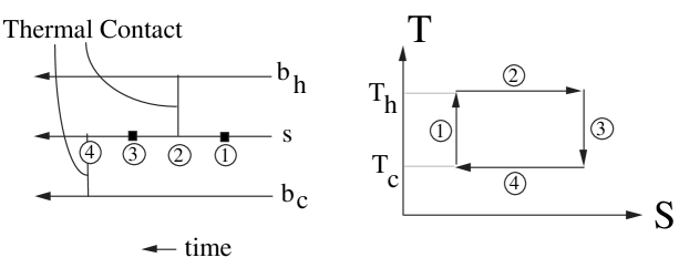
Figure 2: Cycle of a Carnot Engine. Steps 1 (baking $s$) and 3 (cooling $s$) are isentropic, whereas steps 2 and 4 are isothermal.

Appendix B Appendix: Time Reversal of C1 Case

A simple exercise in time reversal is to find the time reversal of the CB net given by Eq.(59), what we called the C1 case of Szilard’s engine. Recall $X=(s,\sigma)$. In our model,

$$P_{{\,\underline{X}\,}_{0}}(X_{0})=\delta_{\sigma_{0}}^{0}P_{{\,\underline{s}\,}_{0}}(s_{0})\;,$$ (107a)

$$P_{{\,\underline{X}\,}_{1}|{\,\underline{X}\,}_{0}}(X_{1}|X_{0})=\delta_{s_{0}}^{s_{1}}P_{{\,\underline{\sigma}\,}_{1}|{\,\underline{s}\,}_{0}}(\sigma_{1}|s_{0})\;,$$ (107b)

and

$$P_{{\,\underline{X}\,}_{2}|{\,\underline{X}\,}_{1}}(X_{2}|X_{1})=\delta_{\sigma_{2}}^{\sigma_{1}}P_{{\,\underline{s}\,}_{2}|{\,\underline{\sigma}\,}_{1}}(s_{2}|\sigma_{1})\;.$$ (107c)

Using Eqs.(107), it is easy to show that

$$P_{{\,\underline{X}\,}^{*}_{2}}(X_{2})=P_{{\,\underline{X}\,}_{2}}(X_{2})=P_{{\,\underline{s}\,}_{2}|{\,\underline{\sigma}\,}_{1}}(s_{2}|\sigma_{2})\sum_{s_{0}}P_{{\,\underline{\sigma}\,}_{1}|{\,\underline{s}\,}_{0}}(\sigma_{2}|s_{0})P_{{\,\underline{s}\,}_{0}}(s_{0})\;,$$ (108a)

$$P_{{\,\underline{X}\,}^{*}_{1}|{\,\underline{X}\,}^{*}_{2}}(X_{1}|X_{2})=P_{{\,\underline{X}\,}_{1}|{\,\underline{X}\,}_{2}}(X_{1}|X_{2})=\delta_{\sigma_{2}}^{\sigma_{1}}\frac{P_{{\,\underline{\sigma}\,}_{1}|{\,\underline{s}\,}_{0}}(\sigma_{2}|s_{1})P_{{\,\underline{s}\,}_{0}}(s_{1})}{\sum_{s_{1}}(num)}\;,$$ (108b)

and

$$P_{{\,\underline{X}\,}^{*}_{0}|{\,\underline{X}\,}^{*}_{1}}(X_{0}|X_{1})=P_{{\,\underline{X}\,}_{0}|{\,\underline{X}\,}_{1}}(X_{0}|X_{1})=\delta_{s_{1}}^{s_{0}}\delta_{\sigma_{0}}^{0}\;.$$ (108c)

Thus the time reversed process has the following CB net

$$\ignorespaces\lx@xy@svg{\hbox{\raise 0.0pt\hbox{\kern 11.56664pt\hbox{\ignorespaces\ignorespaces\ignorespaces\hbox{\vtop{\kern 0.0pt\offinterlineskip\halign{\entry@#!@&&\entry@@#!@\cr&&\\&&\crcr}}}\ignorespaces{{{\hbox{\ellipsed@{11.56662pt}{10.39249pt}}}}\hbox{\kern-11.56664pt\raise 0.0pt\hbox{\hbox{\kern 6.0pt\raise-2.58806pt\hbox{$\textstyle{{\,\underline{s}\,}^{*}_{0}}$}}}}}{{{\hbox{\ellipsed@{11.56662pt}{10.39249pt}}}}\hbox{\kern 35.56664pt\raise 0.0pt\hbox{\hbox{\kern 6.0pt\raise-2.58806pt\hbox{$\textstyle{{\,\underline{s}\,}^{*}_{1}\ignorespaces\ignorespaces\ignorespaces\ignorespaces}$}}}}}\ignorespaces\ignorespaces\ignorespaces{{{}{}{}{}{}}}{{{}{}{}{}{}}}\ignorespaces{}{\hbox{\lx@xy@droprule}}\ignorespaces\ignorespaces\ignorespaces{\hbox{\kern 10.0142pt\raise 5.43056pt\hbox{{}\hbox{\kern 0.0pt\raise 0.0pt\hbox{\hbox{\kern 3.0pt\hbox{\hbox{\kern 0.0pt\raise-2.43056pt\hbox{$\scriptstyle{\delta}$}}}\kern 3.0pt}}}}}}\ignorespaces{\hbox{\kern 11.56975pt\raise 0.0pt\hbox{\hbox{\kern 0.0pt\raise 0.0pt\hbox{\lx@xy@tip{1}\lx@xy@tip{-1}}}}}}{\hbox{\lx@xy@droprule}}{\hbox{\lx@xy@droprule}}{{{\hbox{\ellipsed@{11.56662pt}{10.39249pt}}}}\hbox{\kern 82.6999pt\raise 0.0pt\hbox{\hbox{\kern 6.0pt\raise-2.58806pt\hbox{$\textstyle{{\,\underline{s}\,}^{*}_{2}}$}}}}}{{{\hbox{\ellipsed@{11.56662pt}{10.39249pt}}}}\hbox{\kern-11.56664pt\raise-44.78497pt\hbox{\hbox{\kern 6.0pt\raise-2.58806pt\hbox{$\textstyle{{\,\underline{\sigma}\,}^{*}_{0}}$}}}}}{{{\hbox{\ellipsed@{11.56662pt}{10.39249pt}}}}\hbox{\kern 35.56664pt\raise-44.78497pt\hbox{\hbox{\kern 6.0pt\raise-2.58806pt\hbox{$\textstyle{{\,\underline{\sigma}\,}^{*}_{1}\ignorespaces\ignorespaces\ignorespaces\ignorespaces}$}}}}}\ignorespaces\ignorespaces\ignorespaces{{{}{}{}{}{}}}{{{}{}{}{}{}}}\ignorespaces{}\ignorespaces\ignorespaces\ignorespaces{\hbox{\kern 9.81975pt\raise-50.04053pt\hbox{{}\hbox{\kern 0.0pt\raise 0.0pt\hbox{\hbox{\kern 3.0pt\hbox{\hbox{\kern 0.0pt\raise-2.25555pt\hbox{$\scriptstyle{0}$}}}\kern 3.0pt}}}}}}\ignorespaces{}{{{\hbox{\ellipsed@{11.56662pt}{10.39249pt}}}}\hbox{\kern 82.6999pt\raise-44.78497pt\hbox{\hbox{\kern 6.0pt\raise-2.58806pt\hbox{$\textstyle{{\,\underline{\sigma}\,}^{*}_{2}\ignorespaces\ignorespaces\ignorespaces\ignorespaces\ignorespaces\ignorespaces\ignorespaces\ignorespaces\ignorespaces\ignorespaces\ignorespaces\ignorespaces}$}}}}}\ignorespaces\ignorespaces\ignorespaces{{{}{}{}{}{}}}{{{}{}{}{}{}}}\ignorespaces{}{\hbox{\lx@xy@droprule}}\ignorespaces\ignorespaces\ignorespaces{\hbox{\kern 57.14748pt\raise-39.35442pt\hbox{{}\hbox{\kern 0.0pt\raise 0.0pt\hbox{\hbox{\kern 3.0pt\hbox{\hbox{\kern 0.0pt\raise-2.43056pt\hbox{$\scriptstyle{\delta}$}}}\kern 3.0pt}}}}}}\ignorespaces{\hbox{\kern 58.70302pt\raise-44.78497pt\hbox{\hbox{\kern 0.0pt\raise 0.0pt\hbox{\lx@xy@tip{1}\lx@xy@tip{-1}}}}}}{\hbox{\lx@xy@droprule}}{\hbox{\lx@xy@droprule}}\ignorespaces\ignorespaces\ignorespaces{{{}{}{}{}{}}}{{{}{}{}{}{}}}\ignorespaces{}{\hbox{\lx@xy@droprule}}\ignorespaces{\hbox{\kern 94.26654pt\raise-10.39249pt\hbox{\hbox{\kern 0.0pt\raise 0.0pt\hbox{\lx@xy@tip{1}\lx@xy@tip{-1}}}}}}{\hbox{\lx@xy@droprule}}{\hbox{\lx@xy@droprule}}\ignorespaces\ignorespaces{{{}{}{}{}{}}}{{{}{}{}{}{}}}\ignorespaces{}{{{{}{}{}{}{}}}}\ignorespaces{{{{}{}{}{}{}}}}{{{{}{}{}{}{}}}}\ignorespaces{\hbox{\lx@xy@drawline@}}\ignorespaces{\hbox{\kern 55.07909pt\raise-7.55011pt\hbox{\hbox{\kern 0.0pt\raise 0.0pt\hbox{\lx@xy@tip{1}\lx@xy@tip{-1}}}}}}{{{{}{}{}{}{}}}}\ignorespaces{{{{}{}{}{}{}}}}\ignorespaces{\hbox{\lx@xy@drawline@}}{{{{}{}{}{}{}}}}\ignorespaces{{{}{}{}{}{}}}{\hbox{\lx@xy@drawline@}}\ignorespaces}}}}\ignorespaces\;. \textstyle{{\,\underline{s}\,}^{*}_{0}} \textstyle{{\,\underline{s}\,}^{*}_{1}\ignorespaces\ignorespaces\ignorespaces\ignorespaces} \scriptstyle{\delta} \textstyle{{\,\underline{s}\,}^{*}_{2}} \textstyle{{\,\underline{\sigma}\,}^{*}_{0}} \textstyle{{\,\underline{\sigma}\,}^{*}_{1}\ignorespaces\ignorespaces\ignorespaces\ignorespaces} \scriptstyle{0} \textstyle{{\,\underline{\sigma}\,}^{*}_{2}\ignorespaces\ignorespaces\ignorespaces\ignorespaces\ignorespaces\ignorespaces\ignorespaces\ignorespaces\ignorespaces\ignorespaces\ignorespaces\ignorespaces} \scriptstyle{\delta} \textstyle{{\,\underline{s}\,}^{*}_{0}} \textstyle{{\,\underline{s}\,}^{*}_{1}\ignorespaces\ignorespaces\ignorespaces\ignorespaces} \scriptstyle{\delta} \textstyle{{\,\underline{s}\,}^{*}_{2}} \textstyle{{\,\underline{\sigma}\,}^{*}_{0}} \textstyle{{\,\underline{\sigma}\,}^{*}_{1}\ignorespaces\ignorespaces\ignorespaces\ignorespaces} \scriptstyle{0} \textstyle{{\,\underline{\sigma}\,}^{*}_{2}\ignorespaces\ignorespaces\ignorespaces\ignorespaces\ignorespaces\ignorespaces\ignorespaces\ignorespaces\ignorespaces\ignorespaces\ignorespaces\ignorespaces} \scriptstyle{\delta}$$ (109)

Appendix C Appendix: Binary Symmetric Channels

In this appendix, we will discuss some of the properties of binary symmetric channels. Many results in classical Shannon Information Theory simplify considerably when they are specialized to binary symmetric channels. For instance, the channel capacity is trivial to calculate for such channels.[19]

Throughout this appendix, we will assume $\alpha,\beta,\gamma,\ell\in[0,1]$.

Define the complement of $\alpha$ by

$$\overline{\alpha}=1-\alpha\;,$$ (110)

and the symmetric product of $\alpha$ and $\beta$ by

$$\alpha*\beta=\alpha\beta+\overline{\alpha}\;\overline{\beta}\;.$$ (111)

As shown in Fig.3, the symmetric product has a simple geometrical interpretation in terms of areas contained in the unit square.

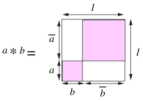
Figure 3: The symmetric product $a*b$ equals the shaded area within the unit square.

One can easily check that the symmetric product is commutative and associative:

$$\alpha*\beta = \beta*\alpha$$ (112a)

$$\alpha*(\beta*\gamma) = (\alpha*\beta)*\gamma\;.$$ (112b)

Other useful properties of the symmetric product are

$$\overline{\alpha}*\beta=1-\alpha*\beta=\overline{\alpha*\beta}\;,$$ (113)

and

$$\alpha*0 = \overline{\alpha}$$ (114a)

$$\alpha*1 = \alpha$$ (114b)

$$\alpha*\frac{1}{2} = \frac{1}{2}\;.$$ (114c)

Define a symmetric matrix by

$$M(\alpha)=\left[\begin{array}[]{cc}\alpha&\overline{\alpha}\\ \overline{\alpha}&\alpha\end{array}\right]\;,$$ (115)

and a symmetric vector by

$$\vec{v}(\ell)=\left[\begin{array}[]{c}\ell\\ \overline{\ell}\end{array}\right]\;.$$ (116)

One can easily check that

$$M(\alpha)\vec{v}(\ell)=\vec{v}(\alpha*\ell)\;,$$ (117)

and

$$M(\beta)M(\alpha)=M(\beta*\alpha)\;.$$ (118)

Define the binary entropy function $h(\alpha)$ by

$$h(\alpha)=-\alpha\ln\alpha-\overline{\alpha}\ln\overline{\alpha}\;.$$ (119)

A binary symmetric channel is defined as the classical Bayesian net ${\,\underline{y}\,}\leftarrow{\,\underline{x}\,}$, where the transition matrix $P_{{\,\underline{y}\,}|{\,\underline{x}\,}}$ is of the form

$$P_{{\,\underline{y}\,}|{\,\underline{x}\,}}=\begin{array}[]{c|cc}&\stackrel{{\scriptstyle x}}{{\scriptstyle 0}}&\stackrel{{\scriptstyle\rightarrow}}{{\scriptstyle 1}}\\ \hline\cr\scriptstyle\downarrow\;0&P(y|x)\\ \scriptstyle y\;1&\\ \end{array}=M(\alpha)\;.$$ (120)

This transition matrix is often represented by the diagram

$$\lx@xy@svg{\hbox{\raise 0.0pt\hbox{\kern 5.5pt\hbox{\ignorespaces\ignorespaces\ignorespaces\hbox{\vtop{\kern 0.0pt\offinterlineskip\halign{\entry@#!@&&\entry@@#!@\cr&&\\&&\crcr}}}\ignorespaces{\hbox{\kern-5.5pt\raise 0.0pt\hbox{\hbox{\kern 0.0pt\raise 0.0pt\hbox{\hbox{\kern 3.0pt\raise 0.0pt\hbox{$\textstyle{0}$}}}}}}}{\hbox{\kern 29.5pt\raise 0.0pt\hbox{\hbox{\kern 0.0pt\raise 0.0pt\hbox{\hbox{\kern 3.0pt\raise 0.0pt\hbox{$\textstyle{}$}}}}}}}{\hbox{\kern 59.5pt\raise 0.0pt\hbox{\hbox{\kern 0.0pt\raise 0.0pt\hbox{\hbox{\kern 3.0pt\raise 0.0pt\hbox{$\textstyle{0\ignorespaces\ignorespaces\ignorespaces\ignorespaces\ignorespaces\ignorespaces\ignorespaces\ignorespaces}$}}}}}}}\ignorespaces\ignorespaces\ignorespaces\ignorespaces{}{\hbox{\lx@xy@droprule}}\ignorespaces\ignorespaces\ignorespaces{\hbox{\kern 51.26105pt\raise 4.50694pt\hbox{{}\hbox{\kern 0.0pt\raise 0.0pt\hbox{\hbox{\kern 3.0pt\hbox{\hbox{\kern 0.0pt\raise-1.50694pt\hbox{$\scriptstyle{\alpha}$}}}\kern 3.0pt}}}}}}\ignorespaces{\hbox{\kern 5.50002pt\raise 0.0pt\hbox{\hbox{\kern 0.0pt\raise 0.0pt\hbox{\lx@xy@tip{1}\lx@xy@tip{-1}}}}}}{\hbox{\lx@xy@droprule}}{\hbox{\lx@xy@droprule}}\ignorespaces\ignorespaces\ignorespaces{}\ignorespaces\ignorespaces{\hbox{\lx@xy@drawline@}}\ignorespaces\ignorespaces\ignorespaces{\hbox{\kern 53.4495pt\raise-9.72246pt\hbox{{}\hbox{\kern 0.0pt\raise 0.0pt\hbox{\hbox{\kern 3.0pt\hbox{\hbox{\kern 0.0pt\raise-2.25555pt\hbox{$\scriptstyle{1-\alpha}$}}}\kern 3.0pt}}}}}}\ignorespaces{\hbox{\kern 5.50002pt\raise-33.36142pt\hbox{\hbox{\kern 0.0pt\raise 0.0pt\hbox{\lx@xy@tip{1}\lx@xy@tip{-1}}}}}}\ignorespaces\ignorespaces{\hbox{\lx@xy@drawline@}}\ignorespaces{\hbox{\lx@xy@drawline@}}{\hbox{\kern-5.5pt\raise-36.44443pt\hbox{\hbox{\kern 0.0pt\raise 0.0pt\hbox{\hbox{\kern 3.0pt\raise 0.0pt\hbox{$\textstyle{1}$}}}}}}}{\hbox{\kern 29.5pt\raise-36.44443pt\hbox{\hbox{\kern 0.0pt\raise 0.0pt\hbox{\hbox{\kern 3.0pt\raise 0.0pt\hbox{$\textstyle{}$}}}}}}}{\hbox{\kern 59.5pt\raise-36.44443pt\hbox{\hbox{\kern 0.0pt\raise 0.0pt\hbox{\hbox{\kern 3.0pt\raise 0.0pt\hbox{$\textstyle{1\ignorespaces\ignorespaces\ignorespaces\ignorespaces\ignorespaces\ignorespaces\ignorespaces\ignorespaces}$}}}}}}}\ignorespaces\ignorespaces\ignorespaces\ignorespaces{}{\hbox{\lx@xy@droprule}}\ignorespaces\ignorespaces\ignorespaces{\hbox{\kern 51.26105pt\raise-40.95137pt\hbox{{}\hbox{\kern 0.0pt\raise 0.0pt\hbox{\hbox{\kern 3.0pt\hbox{\hbox{\kern 0.0pt\raise-1.50694pt\hbox{$\scriptstyle{\alpha}$}}}\kern 3.0pt}}}}}}\ignorespaces{\hbox{\kern 5.50002pt\raise-36.44443pt\hbox{\hbox{\kern 0.0pt\raise 0.0pt\hbox{\lx@xy@tip{1}\lx@xy@tip{-1}}}}}}{\hbox{\lx@xy@droprule}}{\hbox{\lx@xy@droprule}}\ignorespaces\ignorespaces\ignorespaces{}\ignorespaces\ignorespaces{\hbox{\lx@xy@drawline@}}\ignorespaces\ignorespaces\ignorespaces{\hbox{\kern 53.2991pt\raise-26.64433pt\hbox{{}\hbox{\kern 0.0pt\raise 0.0pt\hbox{\hbox{\kern 3.0pt\hbox{\hbox{\kern 0.0pt\raise-2.25555pt\hbox{$\scriptstyle{1-\alpha}$}}}\kern 3.0pt}}}}}}\ignorespaces{\hbox{\kern 5.34668pt\raise-3.0pt\hbox{\hbox{\kern 0.0pt\raise 0.0pt\hbox{\lx@xy@tip{1}\lx@xy@tip{-1}}}}}}\ignorespaces\ignorespaces{\hbox{\lx@xy@drawline@}}\ignorespaces{\hbox{\lx@xy@drawline@}}\ignorespaces}}}}\ignorespaces\;. \textstyle{0} \textstyle{0\ignorespaces\ignorespaces\ignorespaces\ignorespaces\ignorespaces\ignorespaces\ignorespaces\ignorespaces} \scriptstyle{\alpha} \scriptstyle{1-\alpha} \textstyle{1} \textstyle{1\ignorespaces\ignorespaces\ignorespaces\ignorespaces\ignorespaces\ignorespaces\ignorespaces\ignorespaces} \scriptstyle{\alpha} \scriptstyle{1-\alpha} \textstyle{0} \textstyle{0\ignorespaces\ignorespaces\ignorespaces\ignorespaces\ignorespaces\ignorespaces\ignorespaces\ignorespaces} \scriptstyle{\alpha} \scriptstyle{1-\alpha} \textstyle{1} \textstyle{1\ignorespaces\ignorespaces\ignorespaces\ignorespaces\ignorespaces\ignorespaces\ignorespaces\ignorespaces} \scriptstyle{\alpha} \scriptstyle{1-\alpha}$$ (121)

Note that the binary symmetric channel with $P_{{\,\underline{y}\,}|{\,\underline{x}\,}}=M(\alpha)$ is doubly stochastic (the rows and columns of $M(\alpha)$ sum to one). It also satisfies

$$H({\,\underline{y}\,}|{\,\underline{x}\,}) = (P_{\,\underline{x}\,}(0)+P_{\,\underline{x}\,}(1))\left(\alpha\ln\frac{1}{\alpha}+\overline{\alpha}\ln\frac{1}{\overline{\alpha}}\right)$$ (122a)

$$= h(\alpha)\;.$$ (122b)

Claim 15

$$h(\alpha*\ell)\geq h(\ell)\;.$$ (123)

proof: As explained in Ref.[14], if $T_{{\,\underline{y}\,}|{\,\underline{x}\,}}$ is a doubly stochastic transition matrix, then the monotonicity of the relative entropy implies that

$$H(T_{{\,\underline{y}\,}|{\,\underline{x}\,}}P_{\,\underline{x}\,})\geq H(P_{\,\underline{x}\,})\;.$$ (124)

Now set $T_{{\,\underline{y}\,}|{\,\underline{x}\,}}=M(\alpha)$ and $P_{\,\underline{x}\,}=\vec{v}(\ell)$
QED

Consider the model for the C1 case of the Szilard engine which was described in Section 5.1. Let us specialize that model by further assuming that $P_{{\,\underline{s}\,}_{0}}=\vec{v}(\ell)$, $P_{{\,\underline{\sigma}\,}_{1}|{\,\underline{s}\,}_{0}}=M(\alpha)$ and $P_{{\,\underline{s}\,}_{2}|{\,\underline{\sigma}\,}_{1}}=M(\beta)$. Then the table given by Eq.(62) can be expressed in terms of the probabilities $\ell$, $\alpha$ and $\beta$ as follows:

$$\begin{array}[]{l|l|l|}&\hbox{ system }{\,\underline{s}}&\hbox{ system }{\,\underline{s}\,}+\hbox{ sensor }{\,\underline{\sigma}}\\ \hline\cr 1\leftarrow 0&H({\,\underline{s}\,}_{\tau}){|_{\tau=0}^{1}}=&H({\,\underline{s}\,}_{\tau},{\,\underline{\sigma}\,}_{\tau}){|_{\tau=0}^{1}}=\\ &=0&=h(\alpha)\\ \hline\cr 2\leftarrow 1&H({\,\underline{s}\,}_{\tau}){|_{\tau=1}^{2}}=&H({\,\underline{s}\,}_{\tau},{\,\underline{\sigma}\,}_{\tau}){|_{\tau=1}^{2}}=\\ &=h(\beta*\alpha*\ell)-h(\ell)&=h(\beta)+h(\alpha*\ell)-h(\alpha)-h(\ell)\\ \hline\cr 3\leftarrow 2&H({\,\underline{s}\,}_{\tau}){|_{\tau=2}^{3}}=&H({\,\underline{s}\,}_{\tau},{\,\underline{\sigma}\,}_{\tau}){|_{\tau=2}^{3}}=\\ &=-h(\beta*\alpha*\ell)+h(\ell)&=-h(\beta)-h(\alpha*\ell)+h(\ell)\\ \hline\cr 0\leftarrow 3&H({\,\underline{s}\,}_{\tau}){|_{\tau=3}^{0}}=&H({\,\underline{s}\,}_{\tau},{\,\underline{\sigma}\,}_{\tau}){|_{\tau=3}^{0}}=\\ &=0&=0\\ \hline\cr\end{array}$$ (125)

References

- [1] J. C. Maxwell, Theory of Heat (Appleton, London, 1871)
- [2] L. Szilard, Z. Phys. 53, 840 (1929)
- [3] R. Landauer, IBM J. Res. Develop. 5, 183 (1961)
- [4] C. H. Bennett, Int. J. Theor. Phys. 21, 905 (1982)
- [5] T. Sagawa , M. Ueda, “Second Law of Thermodynamics with Discrete Quantum Feedback Control”, arXiv:0710.0956
- [6] T. Sagawa , M. Ueda, “Minimal Energy Cost for Thermodynamic Information Processing: Measurement and Information Erasure”, arXiv:0809.4098
- [7] T. Sagawa , M. Ueda, “Generalized Jarzynski Equality under Nonequilibrium Feedback Control”, arXiv:0907.4914
- [8] S. Toyabe, T. Sagawa , M. Ueda , E. Muneyuki, M. Sano, “Experimental demonstration of information-to-energy conversion and validation of the generalized Jarzynski equality”, arXiv:1009.5287
- [9] T. Sagawa , M. Ueda, “Nonequilibrium thermodynamics of feedback control”, arXiv:1105.3262
- [10] T. Sagawa, “Second Law-Like Inequalities with Quantum Relative Entropy: An Introduction”, arXiv:1202.0983
- [11] K. Funo, Y. Watanabe, M. Ueda, “Thermodynamic Work Gain from Entanglement”, arXiv:1207.6872
- [12] R.R. Tucci, “Counterexamples to the Theory of Thermodynamics With Feedback Proposed By Sagawa and Ueda”, to be published in arXiv.
- [13] R.R. Tucci, “An Introduction to Quantum Bayesian Networks for Mixed States”, arXiv:1204.1550
- [14] R.R. Tucci, “Some Quantum Information Inequalities from a Quantum Bayesian Networks Perspective”, arXiv:1208.1503
- [15] A. Wehrl, Rev. Mod. Phys. 50, 221 (1978)
- [16] R. P. Feynman, Statistical Mechanics: A Set Of Lectures, (Benjamin/Cummings Publishing Company, 1972)
- [17] C. Jarzynski, Phys. Rev. Lett. 78, 2690 (1997); Phys. Rev. E 56, 5018 (1997)
- [18] A.W. Joshi, Elements of Group Theory for Physicists, Second Edition, (Wiley Eastern Limited, New Delhi, 1977)
- [19] T. M. Cover , J. A. Thomas, Elements of Information Theory (John Wiley , Sons, 1991)