Mass transport perspective on an accelerated exclusion process:
Analysis of augmented current and unit-velocity phases

Abstract

In an accelerated exclusion process (AEP), each particle can “hop” to its adjacent site if empty as well as “kick” the frontmost particle when joining a cluster of size $\ell\leq\ell_{\text{max}}$. With various choices of the interaction range, $\ell_{\text{max}}$, we find that the steady state of AEP can be found in a homogeneous phase with augmented currents (AC) or a segregated phase with holes moving at unit velocity (UV). Here we present a detailed study on the emergence of the novel phases, from two perspectives: the AEP and a mass transport process (MTP). In the latter picture, the system in the UV phase is composed of a condensate in coexistence with a fluid, while the transition from AC to UV can be regarded as condensation. Using Monte Carlo simulations, exact results for special cases, and analytic methods in a mean field approach (within the MTP), we focus on steady state currents and cluster sizes. Excellent agreement between data and theory is found, providing an insightful picture for understanding this model system.

I Introduction

Unraveling rich behaviors emerging from simple ingredients in systems driven far from equilibrium is a continuous pursuit in theoretical physics. Non-trivial flux of physical quantities, or current, captures the macroscopic feature of the complex system and is often closely governed by the intrinsic dynamics. There are numerous examples where the steady state current depends sensitively on the constituents in the system through both long-range and short-range interactions such as queueing in traffic and pedestrians Schadschneider et al. (2010), transport of biomolecules Alberts et al. (2004); Epshtein and Nudler (2003); Jin et al. (2010); Lipowsky et al. (2006) and minerals Barrer (1978).

One of the venerable models, the totally asymmetric simple exclusion process (TASEP) not only provides many interesting mathematically exact results of non-equilibrium statistical mechanics Spitzer (1970); Derrida et al. (1992, 1993); Schütz and Domany (1992); Schütz (2001), it also brings insights to potentially important applications in, for example, protein synthesis MacDonald et al. (1968); MacDonald and Gibbs (1969); Klumpp (2011); Chou et al. (2011) and regulating vehicular traffic Chowdhury et al. (2000). Closely related is the zero-range process (ZRP) in which particles hop between sites with rates determined by the origin site occupancy. The mapping between ZRP and an ordinary TASEP proved illuminating in our later discussions. ZRP also finds its versatility in studying granular materials as well as phase separation in one-dimensional systems Evans and Hanney (2005).

Inspired by assisted hopping in transcription Epshtein and Nudler (2003); Jin et al. (2010), we introduced a new variant of TASEP recently Dong et al. (2012), the “accelerated exclusion process” (AEP), to characterize interactions beyond nearest neighbors among particles. Violating detailed balance, AEP is non-equilibrium in nature and involves a few surprising phenomena. Let us briefly recapitulate the dynamic rules of TASEP before turning to the novel features of AEP: In each update attempt of TASEP, a particle in a discrete one-dimensional (1D) lattice of $L$ sites is chosen at random to hop into its neighboring site (provided that is vacant) with rate $\gamma$ (typically chosen as unity). Both periodic and open boundary conditions (particles enter and exit with rates $\alpha$ and $\beta$ respectively) have been studied extensively Spitzer (1970); Derrida et al. (1992, 1993); Schütz and Domany (1992); Schütz (2001). The non-equilibrium steady states of an ordinary TASEP are well-understood. For example, the current-density relationship is given by $J_{\text{TASEP}}=\rho(1-\rho)$, in the thermodynamic limit.

In the AEP with periodic boundary condition, $N$ particles are placed in a ring of $L$ sites and follow the same rules as in TASEP. In addition, when a particle hops to a cluster of particles of size $\ell\leq\ell_{\text{max}}$, it simultaneously “kicks” the frontmost particle of that cluster one site forward. There is no avalanche, as the “kicked” particle does not trigger another kick. When $\ell_{\text{max}}=0$, AEP reduces to an ordinary TASEP. A schematic of AEP is shown in Fig. 1(a).

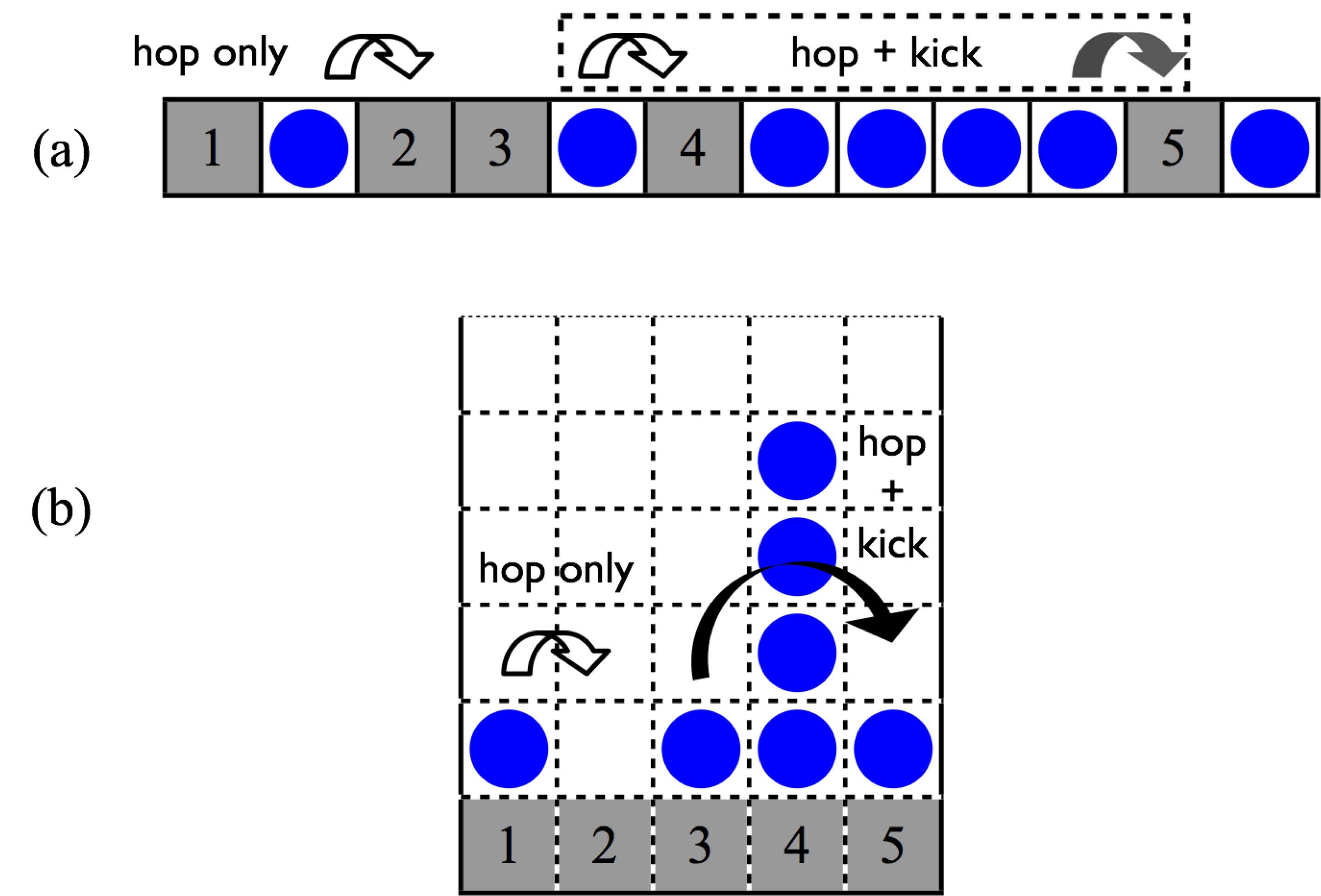
Figure 1: (a) AEP with $\ell_{\text{max}}=4$. A particle can hop (hollow arrows) to its unoccupied right neighboring site and kick (grey arrow) a second particle when joining a cluster of size $\ell\leq\ell_{\text{max}}$. (b) Mapping AEP in (a) to MTP. The ball in stack 3, if chosen, lands immediately in stack 5 ( hop and kick ), while the one in stack 1 lands in stack 2 ( hop ).

In this article, we focus our attention on the non-equilibrium steady states of this AEP and explore the interplay amongst the overall density $\rho\equiv N/L$, $\ell_{\text{max}}$ and current $J(\rho;\ell_{\text{max}})$. Due to “kicking,” a number of novel features arise in the AEP. Given that the contribution to the current can be either 1 (a hop) or 2 (a hop and a kick) Dong et al. (2012), the system is naturally expected to display an augmented current (AC). In this state, the system is homogeneous and we may anticipate that $J_{\text{AC}}$ lies between $J_{\text{TASEP}}$ and $2\times J_{\text{TASEP}}$. It is intriguing that, at high densities ($\rho>1/2$), $J_{\text{AC}}$ can exceed $2\times J_{\text{TASEP}}$. Meanwhile, for low densities, the kicking action results in “facilitated” or “cooperative motion” Antal and Schütz (2000); Gabel et al. (2010); Gabel and Redner (2011), where the average velocity of the particles, $v$, can be increased by adding particles to the system. Clearly absent in the ordinary TASEP, this phenomenon can be characterized by $\partial_{\rho}v>0$ or a positive curvature in $J$: $\partial_{\rho}^{2}J>0$ Antal and Schütz (2000); Gabel et al. (2010); Gabel and Redner (2011). Furthermore, for moderate values of $\ell_{\text{max}}$ and at high densities, the system exhibits an inhomogeneous state in which the particles “condense” into a macroscopic, “solid” cluster, in coexistence with a “fluid” of density $\sim 1/2$. Surprisingly, the (average) current is just $1-\rho=H/L$, where $H$ is the number of holes in the system. Thus, the fluid can be regarded as a loosely bound set of holes, moving together with unit velocity (UV). These two different states of the system will be referred to as the AC and the UV phases, respectively. As the overall density $\rho$ is increased with fixed $\ell_{\text{max}}$, we observe a discontinuous jump in $J(\rho;\ell_{\text{max}})$, from a non-trivial $J_{\text{AC}}(\rho)$ to the simple $J_{\text{UV}}=1-\rho$. Our goal is to understand these remarkable phenomena.

Although AEP is originally cast in the language of an exclusion process, both the intuitive picture and the analysis for predicting the aforementioned features turn out to be much easier when viewed in an equivalent representation, the mass transport process (MTP). In the next Section, we present a detailed description of the AEP-MTP mapping, which is a simple generalization of the TASEP-ZRP mapping. In this setting, the exact master equation can be easily written. Following a brief summary of simulation results in Section III, we provide theoretical considerations for the properties of AC and UV phases in Sections IV and V, respectively. In Section VI, we venture a phase diagram for this system. We conclude and provide an outlook for further quests in Section VII.

II Accelerated Exclusion as a Mass Transport Process

Regarded as particles traversing a 1D ring, AEP allows particle to move only when it is adjacent to a hole. The configuration of the system, $\mathcal{C}$, can be characterized by the set of site occupancies, $\{n_{i}\},i=1,...,L$, with $n$ being 0 or 1. Alternatively and more conveniently, AEP can be formulated as a mass transport process (MTP) Kafri et al. (2002) in which we regard the particles in front of each hole as “balls” stored in a “stack.” Each hole in AEP becomes a stack in MTP, labeled by $\alpha=1,...H$. The $\ell_{\alpha}$ balls in stack $\alpha$ correspond to the cluster of particles between the $\alpha^{\text{th}}$ and $(\alpha+1)^{\text{th}}$ hole. Each stack may be occupied by any number of (indistinguishable) balls: $\ell_{\alpha}=0,1,...,N$. An equivalent specification of $\mathcal{C}$ can thus be the set $\left\{\ell_{\alpha}\right\}$ instead.

The mapping from AEP in Fig. 1(a) to MTP is shown in Fig. 1(b). The dynamic rules of AEP thus become: In each update attempt, a random stack $\alpha$ is chosen. If it is empty ($\ell_{\alpha}=0$), another attempt is made. Otherwise, one of the balls in the chosen stack hops to the next stack and if $\ell_{\alpha+1}\in\left[1,\ell_{\max}\right]$, the ball takes a second hop immediately, landing in stack $(\alpha+2)$. For instance, the “hop and kick” scenario in Fig. 1(a) becomes a hop from stack 3 to 5 in Fig. 1(b). When $\ell_{\text{max}}=0$, it returns to an ordinary TASEP.

Clearly, $N=\Sigma_{\alpha}\ell_{\alpha}$ is conserved. These rules are summarized in the master equation for $P\left(\mathcal{C};t\right)$ in Eq. (1). One of the advantages of MTP representation is that $\left\{\ell_{\alpha}\right\}$ provides directly the cluster size distribution in the AEP, a measure which we can use to characterize the AC and UV phases quantitatively.

The only non-trivial aspect of this mapping is $J$, the overall particle current. In each update attempt, a random site is chosen for AEP, while in MTP is a stack. Thus, the time scale differs by a factor of $H/L$. In particular, if we compute the average number of particle movements in MTP, it must be multiplied by $H/L=1-\rho$ when compared to $J$ in AEP.

We proceed to formulating the dynamic rules as a master equation. To facilitate this task, we define the characteristic functions

$$\chi\left(\ell\right) \equiv 1~{}~{}\text{if}~{}\ell\in\left[1,\ell_{\max}\right];~{}~{}0~{}~{}\text{otherwise}.$$

$$\overline{\chi}(\ell) \equiv 1-\chi(\ell)$$

Note that $\ell_{\max}$ is an implicit parameter in these functions. The master equation governing the evolution of $P\left(\mathcal{C};t\right)$, namely the probability to find the system in configuration $\mathcal{C}=\left\{\ell_{a}\right\}$ in $t$ attempts after some initial configuration, for $H>2$ is:

$$\begin{split}P\left(\mathcal{C}^{\prime};t+1\right)=&\sum_{\mathcal{C}}\dfrac{1}{H}\sum_{\alpha=1}^{H}P\left(\mathcal{C};t\right)\left[\prod\limits_{\beta\neq\alpha,\alpha+1,\alpha+2}\delta\left(\ell_{\beta}^{\prime},\ell_{\beta}\right)\right]\delta\left(\ell_{\alpha}^{\prime},\ell_{\alpha}-1\right)\times\\ &\times\left\{\delta\left(\ell_{\alpha+1}^{\prime},\ell_{\alpha+1}\right)\delta\left(\ell_{\alpha+2}^{\prime},\ell_{\alpha+2}+1\right)\chi\left(\ell_{\alpha+1}\right)+\delta\left(\ell_{\alpha+1}^{\prime},\ell_{\alpha+1}+1\right)\delta\left(\ell_{\alpha+2}^{\prime},\ell_{\alpha+2}\right)\overline{\chi}\left(\ell_{\alpha+1}\right)\right\}\end{split}$$ (1)

Here, $\delta$ is the Kronecker delta. For $H=1$, there is just one stack in MTP, leaving AEP trivial. For $H=2$, the problem is easily solvable and hints at the significant role of $\ell_{\max}$. The next case ($H=3$) is the first non-trivial one and the exact solution in the $L\rightarrow\infty,\ell_{\max}\rightarrow\infty$ limit provides valuable insight into the UV phase. We show the details of $H=2$ and 3 in Appendices A and B.

The configuration space $\left\{\ell_{\alpha}\right\}$ consists of the lattice points in an $(H-1)$-dimensional hyper-tetrahedron. The easiest way to visualize this is its standard embedding in $H$-dimension, i.e., a (linear) space joining the following $H$ points: $(N,0,...,0),...,(0,...,0,N)$. For $H=3$ and 4, the configuration space is just an equilateral triangle and the standard regular tetrahedron, respectively.

In general, this dynamics does not obey detailed balance, so that finding an explicit stationary distribution, $P^{*}\left(\mathcal{C}\right)$, is not simple Zia and Schmittmann (2007); Hill and Kedem (1966). To have some understanding of the system behavior, we will exploit the approximation schemes presented below, before which let us comment briefly on some general properties of our system.

Two extreme cases are noteworthy. One is $\ell_{\max}=0$, which is simply the ordinary TASEP. Dropping the $\chi$ term, Eq.(1) reduces to

$$\begin{split}P_{\text{TASEP}}\left(\mathcal{C}^{\prime};t+1\right)=\sum_{\mathcal{C}}\frac{1}{H}\sum_{\alpha=1}^{H}P_{\text{TASEP}}\left(\mathcal{C};t\right)\times~{}~{}~{}\\ \times\delta\left(\ell_{\alpha}^{\prime},\ell_{\alpha}-1\right)\delta\left(\ell_{\alpha+1}^{\prime},\ell_{\alpha+1}+1\right)\prod\limits_{\beta\neq\alpha,\alpha+1}\delta\left(\ell_{\beta}^{\prime},\ell_{\beta}\right)\end{split}$$ (2)

Though this dynamics also violates detailed balance, it does satisfy the “pairwise balance” condition Spitzer (1970), so that $P_{\text{TASEP}}^{\ast}\left(\mathcal{C}\right)\propto 1$. The opposite extreme is $\ell_{\max}\rightarrow\infty$, or simply $\ell_{\max}>L$ or $N$. $\overline{\chi}\left(\ell\right)$ reduces to $\delta\left(\ell\right)$ so that $\left\{...\right\}$ in Eq. (1) becomes:

$$\begin{split}\{&\delta\left(\ell_{\alpha+1}^{\prime},\ell_{\alpha+1}\right)~{}~{}~{}\delta\left(\ell_{\alpha+2}^{\prime},\ell_{\alpha+2}+1\right)\overline{\delta}\left(\ell_{\alpha+1},0\right)+\\ +&\delta\left(\ell_{\alpha+1}^{\prime},\ell_{\alpha+1}+1\right)\delta\left(\ell_{\alpha+2}^{\prime},\ell_{\alpha+2}\right)\delta\left(\ell_{\alpha+1},0\right)\}\end{split}$$ (3)

where $\overline{\delta}\equiv 1-\delta$. This important limit exemplifies the AC phase and will be examined more closely below.

Returning to the general case, one can compute the average of any quantity ${\cal Q}$ in the stationary state assuming $P^{\ast}$ is known:

$$\left\langle{\cal Q}\right\rangle\equiv\sum{\cal Q}P^{\ast}$$

where the sum is taken over $\left\{n_{i}\right\}$ or $\left\{\ell_{\alpha}\right\}$, whichever is more convenient. In particular, the average particle current in steady state is given by:

$$\begin{split}J\left(\rho;\ell_{\max}\right)&=\left\langle n_{1}\left(1-n_{2}\right)\left(1+n_{3}\right)\right\rangle\\ &~{}~{}~{}~{}~{}-\left\langle n_{1}\left(1-n_{2}\right)\prod\limits_{m=0}^{\ell_{\max}}n_{3+m}\right\rangle\\ &=\left(1-\rho\right)\left\langle\overline{\delta}\left(\ell_{1},0\right)\left[1+\chi\left(\ell_{2}\right)\right]\right\rangle\end{split}$$ (4)

Note that we have invoked translational invariance of $P^{\ast}$ in writing these expressions. If the reader is concerned that this invariance may be (spontaneously) broken, as in the UV phase, then $J=\sum_{\left\{n\right\}}\left\langle...\right\rangle/L=$ $\sum_{\left\{\ell\right\}}\left\langle...\right\rangle/H$ may be used instead. Also, the second line is the result of having one (two) hop(s) for a particle-hole-hole(particle-hole-particle) triplet. In MTP, whenever stack 1 is chosen, a ball will hop, with an additional hop if the target stack has the requisite number of balls.

III Simulation results

We exploit the random sequential updating scheme and simulate AEP with a typical lattice of $L=1000$. Initializing the system with $N$ particles on successive lattice sites, we make $N$ attempts to update in every Monte Carlo step (MCS) so that each particle has on average one chance to hop. The contribution to the current from both hops and kicks are instantly accounted for. The typical length of our simulations is $\tau=5\times 10^{5}$ MCS. We start data collection after $2\times 10^{5}$ MCS to ensure that the system has reached steady state and all measurements are averaged over $3\times 10^{5}$ MCS thereafter unless otherwise specified.

Figure 2: (Color online) Comparison amongst $J_{\text{AC}}$ from Monte Carlo simulation, $J_{\text{TASEP}}$, $2J_{\text{TASEP}}$, a naïve mean field approximation and an improved mean field approximation through MTP (MTP-MF). The result from MTP-MF in Eq. (11) (blue solid line) provides remarkable agreement with the simulation.

Figure 3: (Color online) Curvature of $J(\rho)$ from simulation (circles), a naïve mean field approximation (blue dotted line) and MTP-MF (blue solid line).

First let us examine the AC phase. We note that not only is $J$ always larger than $J_{\text{TASEP}}$ except at $\rho=0$ and 1, it even surpasses $2J_{\text{TASEP}}$ when $\rho>1/2$, as shown in Fig. 2. The simulation (red circles) is for $\ell_{\text{max}}=1000$ and thus all hops lead to kicks. The system is always in the AC phase regardless of the density, which may lead one to believe that $J_{\text{AC}}$ should be close to $2J_{\text{TASEP}}=2\rho\left(1-\rho\right)$, since a typical particle will hop two sites instead of just one. This rough estimate is reasonably good for high densities, as Fig. 2 (black dot-dash line) indicates. Using the most naïve mean field approximation, we can start from the exact expression Eq. (4) and let $\ell_{\max}\rightarrow\infty$. This leads us to $\rho\left(1-\rho^{2}\right)$. Surprisingly, this provides a much poorer overall picture (blue dotted line in Figs. 2 and 3). Furthermore, there is some inflection at low density where the curvature of $J_{\text{AC}}(\rho)$ is positive, indicating an “accelerated region.” This is illustrated in Fig. 3.

Utilizing the MTP picture, we provide a mean field theory (MTP-MF) in Section IV to describe the AC phase, which yields exceptional agreement with simulation data, shown in solid blue line in Figs. 2 and 3. This approach leads to a remarkably good description of all phenomena presented here. Moreover, it provides a viable explanation for why the estimate $\rho\left(1-\rho^{2}\right)$ fails. The details are presented in Section IV.

The emergence of the UV phase depends on the appropriate choice of $\ell_{\text{max}}$. In all of our simulations where $L=1000$, there exists a UV phase for $10\lesssim\ell_{\text{max}}\lesssim 950$. We show a few typical $\ell_{\text{max}}$’s in Fig. 4. When the system enters UV, $J$ becomes independent of $\ell_{\text{max}}$ and is simply $(1-\rho)$, indicating the holes are moving at average speed 1. It is therefore both more effective and illuminating to switch to the reference frame of moving holes: Starting from a full system with one giant cluster of particles, i.e. $H=0$, as more and more holes are injected to the system, we find the system settles into a cluster of particles in one part and a half-filled region in the other part of the system. Exploiting both AEP and MTP frameworks, we explicate the emergence of such “phase separation” in Section V.

Figure 4: (Color online) Transition from AC to UV for $\ell_{\text{max}}=20$ (red circles), 100 (green squares) and 500 (yellow triangles).

IV Augmented Current Phase: Mean Field Description

In this section, we focus on the stationary state of the AC branch, in which the system is homogeneous and the density profile is just $\rho$. Now, if we let $\ell_{\max}>L$, then the system be in AC for all $\rho$’s. In the MTP representation, the rule is especially straightforward: Every hop into an occupied stack makes a further hop. Thus, the probability that a stack is occupied

$$f\equiv\left\langle\overline{\delta}\left(\ell_{1},0\right)\right\rangle$$

will play a central role. Further, we find it useful to study the more detailed distribution

$$P^{*}\left(\ell\right)\equiv\left\langle\delta\left(\ell,\ell_{1}\right)\right\rangle$$

i.e., the probability that a stack contains precisely $\ell$ particles. Of course, $f=\sum_{\ell>0}P^{*}\left(\ell\right)$ implies

$$1-f=P^{*}\left(0\right).$$ (5)

IV.1 Steady state occupations

Although it is not possible to derive an exact master equation for $P\left(\ell;t\right)\equiv\sum\delta\left(\ell,\ell_{1}\right)P\left(\mathcal{C};t\right)$ from Eq. (1), we will exploit a mean field approach to find $P^{\ast}\left(\ell\right)$. To maintain a steady state, a given stack must gain and lose a ball with equal probability in any attempt. In other words, we can find $P^{\ast}$ by balancing the average rates of gain and loss.

Clearly, the probability that an occupied stack ($\ell\geq 1$) loses a ball is $P^{\ast}\left(\ell\right)$ (with the trivial factor of $1/H$ suppressed). Meanwhile, the stack can gain one ball (i.e., $\ell-1\rightarrow\ell$) if both stacks upstream are occupied. Injecting the mean field approximation, we estimate this condition by $f^{2}$. If the chosen stack is empty, there is an additional way it can gain, from its immediate upstream neighbor if occupied. Thus, the balance equations read:

$$\left(f^{2}+f\right)P^{\ast}\left(0\right) = P^{\ast}\left(1\right)$$

$$f^{2}P^{\ast}\left(\ell\right) = P^{\ast}\left(\ell+1\right);\,\ell>0.\,\,$$

Strictly, we should account for the upper limit $\ell\leq N$. If we neglect such finite size size effects, the normalization constraint is $\Sigma_{\ell=0}^{\infty}P^{\ast}\left(\ell\right)=1$, leading us to an explicit expression for the stationary distribution:

$$P^{\ast}\left(\ell>0\right) = \left(1+f\right)f^{2\ell-1}P^{\ast}\left(0\right)$$ (6)

$$P^{\ast}\left(0\right) = 1-f$$ (7)

Note that Eq. (7) is entirely consistent with Eq. (5).

Next, let us relate $f$ to the density $\rho$. Computing $\left\langle\ell\right\rangle$ is straightforward: $f/\left(1-f^{2}\right)$. But this average occupation must be $N/H=\rho/\left(1-\rho\right)$, leading to

$$f^{2}+\frac{H}{N}f=1$$ (8)

Instead of a cumbersome algebraic expression for $f\left(\rho\right)$, let us define $\eta$ by

$$\sinh\eta\equiv\frac{H}{2N}=\frac{1-\rho}{2\rho}$$ (9)

and recognize $\left(1-f^{2}\right)/f=f^{-1}-f$, so that

$$f=e^{-\eta}$$ (10)

or explicitly, $f=\exp\left\{-\sinh^{-1}\dfrac{1-\rho}{2\rho}\right\}$ . Not surprisingly, $f$ is a monotonically increasing function of $\rho$.

In the next subsection, we exploit these results to find the current-density relationship and explore some consequences.

IV.2 Currents and velocities

In MTP, an occupied stack ($f>0$) contributes one (or two) hop depending on whether the next stack is empty (or occupied), the probability of which is associated with $\left(1-f\right)$ (or $f$). Within our approximate scheme, the total contribution is $f\left[\left(1-f\right)+2f\right]=f\left(1+f\right)$. Together with the $H/L$ factor to scale from MTP to AEP, we conclude that the mean field approximation for the particle current is

$$J_{\text{AC}}^{\text{MTP-MF}}\left(\rho\right)=\left(1-\rho\right)f\left(1+f\right)$$ (11)

This simple approximation provides an excellent prediction, with no fit parameters. The solid blues line in Figs. 2 and 3 show its remarkable agreement with our simulation data.

Recall $\rho\left(1-\rho^{2}\right)$, the “naïve mean field approximation” for $J\left(\rho\right)$, which is far from simulation data (see Fig. 2 except near $\rho=0,1$). What is the difference between the two approaches - that one performs so much better? Comparing Eq. (11) with $\rho\left(1-\rho^{2}\right)$, we see the difference to be simply $f\left(1+f\right)$ instead of $\rho\left(1+\rho\right)$. Since $f$ is an estimate of the probability of successive holes not being nearest neighbors, the failure of $\rho$ here implies that it underestimates much of the clustering of the particles,. The remedy provided by MTP can be cast as a simple and intuitive picture, for which we coin the phrase “abhorrence of empty stacks.” Since an empty stack can be filled by hops from two (upstream) stacks, it is far less likely to remain empty, compared to the situation in the ordinary TASEP. It is easy to check that $f-\rho$ is positive for $\rho\in\left(0,1\right)$ and peaks at $\thicksim 0.12$ (around $\rho\thicksim 0.57$). In other words, $f$ is more successful at accounting for the scarcity of empty stacks, consecutive holes in AEP language (at moderate densities).

Now let us consider “velocity.” There are two notions of velocity associated with $J\left(\rho\right)$. One is the average particle velocity, $v=J/\rho$. From Eq. (11), we obtain a simple expression:

$$v^{\text{MTP-MF}}=J/\rho=\left(1-f^{2}\right)\left(1+f\right)$$ (12)

Since particles never hop backwards, this $v$ is necessarily positive, approaching $1$ (or $0$) in the limit $\rho\rightarrow 0$ (or $1$).

The other notion of velocity is $\partial_{\rho}J$. Similar to the group velocity for waves, $\partial_{\rho}J$ is sensitive to collective behavior such as the motion of fluctuations or disturbances. Thus, it is negative at high densities, corresponding to holes moving “backwards” (the simplest case being the single-hole system). An unusual and notable feature of AEP is “cooperative motion” Antal and Schütz (2000); Gabel et al. (2010); Gabel and Redner (2011). In an ordinary TASEP, adding a particle to the system always reduces both $v$ and $\partial_{\rho}J$. In AEP, by contrast, there is a regime in which particles “cooperate” and move faster when more are present: Namely both $\partial_{\rho}v$ and $\partial_{\rho}^{2}J$ can be positive. Both simulation data and $\partial_{f}v^{\text{MTP-MF}}=\left(1+f\right)\left(1-3f\right)$ display such a regime. Similarly, this behavior is also present in $\partial_{\rho}^{2}J$, studied in Antal and Schütz (2000); Gabel et al. (2010); Gabel and Redner (2011) and easily discerned as curvature shown in Fig. 3. Given the agreement in Fig. 2, it is not surprising that the MTP-MF is also successful at predicting the phenomenon of cooperative motion.

Additionally, let us comment on two other features associated with the current $J_{\text{AC}}^{\text{MTP-MF}}\left(\rho\right)$. It is clear from Eq. (8) that, at $\rho=0.5$, we have $N=H$ and so $f\left(1+f\right)=1$. Inserting this result into Eq. (11), we conclude that $J_{\text{AC}}^{\text{MTP-MF}}\left(0.5\right)=0.5$. This is larger than simulation data by about $1\%$, a difference which may be attributed to either statistical errors in the data or MTP-MF’s failure to capture certain correlations. Since our system does not obey explicit particle-hole symmetry, it is unclear if $J=0.5$ is merely a curious coincidence or an indication of some hidden symmetry. Of course, this is the “maximal” value of $2J_{\text{TASEP}}$, but again, this coincidence may also be accidental. Finally, we note that both the data and $J_{\text{AC}}^{\text{MTP-MF}}$ exceeds $2J_{\text{TASEP}}$ for much of $\rho>1/2$, both peaking around $\rho\cong 0.54$. Apart from the mathematical analysis, we have not developed a good intuitive picture for explaining these observations.

IV.3 Cluster size distribution

Exploiting the MTP-MF further, we can compare the result in Eq. (6) with measurements of the cluster size distribution (CSD). In Fig. 5, we show simulation data for $N=600$ and 900, both with $\ell_{\max}=1000$. It is clear that the distributions are consistent with exponentials. Further, if we construct ratios of the successive values, we find the average over a range (where the scatter of the data is small) to be $0.556$ and $0.895$, respectively. For comparison, using Eqs. (9, 10) to compute $f^{2}$, we find the values being $0.519$ and $0.895$, respectively. Another point for comparison is $P^{\ast}\left(0\right)$, for which the simulation data provide $0.291$ and $0.0582$ versus $0.279$ and $0.0540$ from Eqs. (7, 9, 10), respectively. Such agreement leads us to conclude that the MTP-MF approach indeed captures the essence of the AC phase.

Figure 5: (Color online) Cluster size distributions in AC phase. $\ell_{\text{max}}=L=1000$ with $N=$ 600 (magenta diamond) and 900 (black triangle), respectively. Theoretical predictions are not shown explicitly for clarity. The agreement between them and data are comparable to those in Figs. 2 and 3.

V Unit Velocity Phase: Perspectives from both AEP and MTP

In this section, we focus on the UV branch, in which the system is inhomogeneous and exhibits an approximately half-filled region in coexistence with a fully occupied domain. The presence of this phase depends crucially on having a moderate $\ell_{\max}$. The most remarkable feature of this phase is that the average particle current is exactly $(1-\rho)$, shown in Fig. 4. In other words, the average speed of the holes (or the “disturbances” ) is precisely $1$, independent of particles being added to, or removed from, the system (until a phase boundary is reached). In both AEP and MTP representations, there exist simple descriptions which provide an intuitive and appealing picture for why such an unusual state can persist. The following subsections are devoted to each of these perspectives. Before presenting the details, note that such a state spontaneously breaks the translational symmetry underpinning the dynamics. Interestingly, this broken symmetry is manifested in slightly different forms in the two representations. We will comment on this difference in each of the subsections below.

V.1 A “hole train” in AEP

In the language of the original exclusion process, this phase is best understood if we focus on how the holes move. When we choose the particle at site $k-1$ and find that it can hop to a hole at site $k$, we can regard this process as choosing the hole and exchanging it with the partner particle. Next, we should ask if there is a (particle) cluster of length $\ell$ occupying the sites from $k+1$ on. When $\ell\in\left[1,\ell_{\max}\right]$, we also move the hole at $k+\ell+1$ to $k+\ell$. In other words, when a hole moves, it will pull the next hole (“downstream”), provided the gap between them lies in $\left[1,\ell_{\max}\right]$. We should remind the reader that the second hole does not pull a third one.

Since this phase is present only in the high density regime, it is natural to first consider systems with the lowest values of $H$. These provide us the necessary picture to understand the existence of a UV phase. A system with a single hole evolves trivially: The hole “swims upstream” with unit average velocity, since every attempt to move it is successful. The $H=2$ case is somewhat more interesting. Deferring the details to Appendix A, we state the principal results here. It is straightforward to enumerate, for any $L$ and $\ell_{\max}$, all possible stationary states, through which the important role played by $\ell_{\max}$ is revealed. Most significantly, for moderate $\ell_{\max}/L$, the two holes form a tightly bound pair. To be precise, the gap between them can be either $0$ or $1$, with equal probability. Let us emphasize that this is an absorbing state. Starting with any initial separation, the two holes will eventually drift together, form the bound state, and never become unbound thereafter. Since the “leading” hole always moves when it is chosen, the pair moves with unit average velocity.

The first non-trivial case is $H=3$. For a finite system with arbitrary $\ell_{\max}$, an exact solution is not yet available. Nevertheless, we can gain some insight into the UV behavior through an exact result in the limit $L\rightarrow\infty$ followed by $\ell_{\max}\rightarrow\infty$ (details in Appendix B). Here, the leading pair remains tightly bound, as the third hole cannot affect the leading hole. Denoting the gap between the second and the third hole by $m$, we know that the third hole can trail behind the second by $m\geq 0$, so that the complete description of the system lies in the following probabilities. Let $p_{0,1}\left(m\right)$ be the probability that the gap between the first hole pair is $0$ or $1$, with the third hole trailing by $m$ sites. We illustrate examples of $p_{0}\left(5\right)$ and $p_{1}\left(4\right)$ in Fig. 6. As shown in Appendix B, we find (apart from $m=0,1$)

$$p_{0,1}\left(m\right)\propto\zeta^{m}$$ (13)

where $\zeta=2-\sqrt{2}\cong 0.586$. In other words, the third hole is “loosely” bound, with an exponential tail of a characteristic length $\mu\equiv-1/\left(\ln\zeta\right)\cong 1.87$. The intuitive picture is clear: The first pair advances with UV, with the third hole being “pulled along,” at a typical distance $\mu$ behind the second. It is natural to label such a triplet a “hole train” with the first pair being the “engine”Dong et al. (2012).

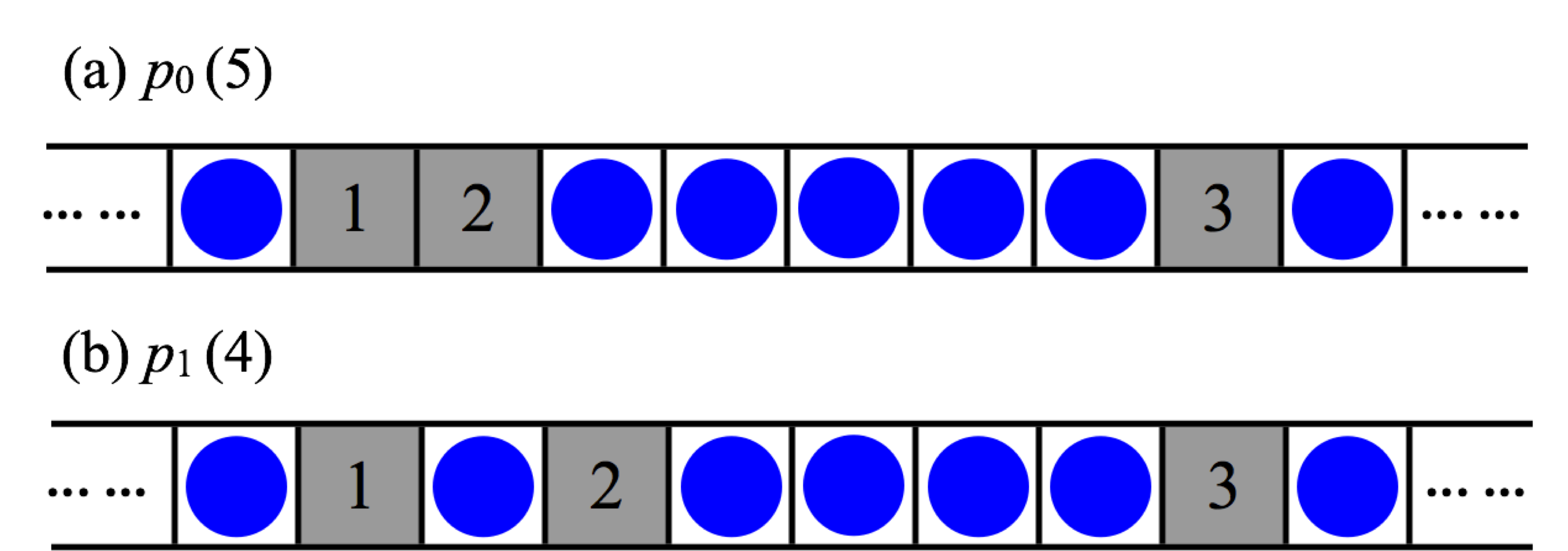
Figure 6: Sketch of a “hole-train” with $H=3$: (a) Two leading holes are consecutive with the third trailing by $m=5$. The probability of this scenario is denoted as $p_{0}(5)$. (b) Two leading holes have one particle in between, with the third trailing by $m=4$, denoted as $p_{1}(5)$.

Continuing this line of thought, we see that, in the limit posed above, the first pair will always form an “engine” which advances with UV, unaffected by how many holes trail behind them. While we do not have exact solutions for the general case, we can argue why the holes should be bound and the image of a train is quite reasonable. In particular, consider the last hole – the “caboose” in the parlance of freight trains – and the penultimate hole, which we will refer to as “X.” If X is chosen and moves, it will pull the caboose along (provided the gap in-between is non-zero). The gap remains the same. On the other hand, if the caboose moves, the gap decreases. Only when X is pulled along by the hole upstream from it does the gap increase. Although these considerations appear to imply that the gap between penultimate and final holes performs a typical random walk, we point out that the entire train length does not increase even when this gap increases. Thus, we argue that this mechanism can “hold the train together.” Accepting this scenario, we see that adding or removing holes to the system merely changes the total length of the train. Meanwhile, since the engine advances with UV, the whole train also moves as such, leading to an $H$-independent velocity. In the following section, we present a more tenable and quantitative argument for the existence of this hole train, as well as an estimate of its average density ($\thicksim 0.5$) in the language of MTP.

Before proceeding, let us comment on two other aspects of the AEP perspective. First, although a typical snapshot of our system clearly violates translational invariance, this symmetry is restored quite quickly ($O\left(L\right)$ MCS) since the hole-train moves at UV. To be precise, if we measure the occupation at a specific site, it will settle at $\rho$ within such times. If, on the other hand, we tag a particular hole and measure the occupation in one of its nearest neighbor sites, then the results will expose the inhomogeneity inherent in the system. Restoration of the symmetry (in finite systems) would take much longer than $O\left(L\right)$ MCS, a subject well beyond the scope of this work. Second, in a finite periodic lattice, the average distance between the caboose and the engine, $\Delta$, is finite. For systems with $\Delta\gg\ell_{\max}$ , the caboose does not affect the (lead hole in the) engine. Thus, the integrity of the engine remains intact and moves the entire train with UV. As holes are added or removed, $\Delta$ becomes smaller or larger, respectively. When enough holes are added, or if $\ell_{\max}$ is raised, then $\Delta$ can approach $\ell_{\max}$, the caboose can destroy the engine, and the train can become unbound. In a nutshell, this is the mechanism for the transition from UV to AC, as the overall density is lowered (e.g., Fig. 4). We will return to this picture in Section VI.

V.2 Condensation in MTP

As for the AC phase, the MTP representation provides us with a more quantitative picture. The solid particle cluster plays the role of the condensate in non-trivial ZRP’s. With a finite (and small enough) $\ell_{\max}$, it is possible for one stack to contain more balls than $\ell_{\max}$. Such a stack can gain balls in two possible ways, much like how an empty stack can be filled above. Meanwhile all stacks can lose a ball in just one way. Thus, the number in this stack will grow, until a steady state is reached. It is natural to refer to this behavior as “condensation” and this stack (or the balls in this stack) as the “condensate.” To make contact with the previous subsection, note that there are $\Delta$ balls in the condensate stack. Needless to say, each of the remaining $H-1$ stacks is likely to hold very few balls. In the language of ZRP, the state of the other stacks is referred to as “a fluid.” Here, we recognize them as the hole train. Further, this picture allows us to appreciate better why the hole train remains bound. First, the train length is monotonically related to the fluid density, becoming longer/shorter when the condensate loses/gains balls. Second, the only way to redress the imbalance (two gains vs. one loss) for the condensate is when the fluid density remains relatively low, i.e., a set of stacks with few balls in each. This scenario corresponds to a bound train.

Turning to a more quantitative description of the steady state, we denote the occupation probability within the train by $f_{\text{train}}$. A good estimate for it comes from the balance of the gain/loss contributions from the condensate, namely

$$f_{\text{train}}+f_{\text{train}}^{2}=1$$ (14)

The predicted value, $f_{\text{train}}=\left(\sqrt{5}-1\right)/2$, is not very illuminating. Instead, by comparing with Eq. (8), we find a more insightful relation:

$$H_{\text{train}}=N_{\text{train}}$$ (15)

namely, $\rho_{\text{train}}=0.5$, implying a train length is $2H_{\text{train}}$. This result also indicates that the typical distance from one hole to the next in the train is around $2$, a picture entirely consistent with the result $\mu\thicksim 2$ in the $H=3$ case.

Meanwhile, since the train consists of $H-1$ stacks, we arrive at $H_{\text{train}}\cong H$. Further, we have $N_{\text{train}}+\Delta=N=L-H$ so that the size of the condensate is given by:

$$\Delta\cong L-2H=L\left(2\rho-1\right)$$ (16)

All these predictions are borne out relatively well in simulations. For example, in Fig. 7, we show the CSD’s for $N=600$ and $900$ with $\ell_{\text{max}}=100$. Clearly, the condensate sizes are seen to fluctuate around $200$ and $800$ respectively, as predicted by Eq. (16). The properties of the fluid/hole-train, as revealed by the small clusters not shown in Fig. 7, are essentially the same in both cases. For small clusters the distribution indeed decays exponentially, with ratios of the successive values being $0.406$ and $0.412$, respectively. These are somewhat higher than $f_{\text{train}}^{2}\cong 0.382.$ Given that our theory is based on a mean field approximation, we speculate that the difference are due to non-trivial correlations, the study of which is beyond the scope of this work.

So far, the analysis is focused on the average behavior of the fluid and the condensate. Since our approach considers the single-stack occupation, we can apply it to the condensate and exploit a self-consistent way to predict $P^{\ast}_{\text{con}}\left(\Lambda\right)$, the probability for the condensate to have $\Lambda$ balls in the steady state. Note that, unlike $\Delta$, $\Lambda$ is a variable here. In such a configuration, the fluid has only $N-\Lambda$ balls, which allows us to estimate $\tilde{f}$ (the occupation probability of a stack in the fluid) as a function of $\Lambda$. Using Eqs.  (9,10), we find $\tilde{f}\left(\Lambda\right)=\exp\left\{-\sinh^{-1}\frac{H-1}{2\left(N-\Lambda\right)}\right\}$ while $\tilde{f}\left(\Delta\right)$ is just $f_{\text{train}}$. We can now use $\tilde{f}$ to estimate the rate at which the fluid supplies a ball to the condensate, namely, $\tilde{f}^{~{}2}+\tilde{f}$. Denoting this rate by

$$g\left(\Lambda\right)\equiv\tilde{f}^{~{}2}+\tilde{f}$$ (17)

we find an expression similar to Eq. (IV.1)

$$g\left(\Lambda\right)P^{\ast}_{\text{con}}\left(\Lambda\right)=P^{\ast}_{\text{con}}\left(\Lambda+1\right),$$ (18)

since the condensate loses at unit rate. It is straightforward to check that $g\left(\Lambda\right)$ is a monotonically decreasing function and is unity at $\Lambda=\Delta$. Thus, $P^{\ast}_{\text{con}}\left(\Delta+1\right)=P^{\ast}_{\text{con}}\left(\Delta\right)\equiv\hat{P}$ are the peak values of the distribution and can be conveniently used to start the recursive evaluation of two sequences: $P^{\ast}_{\text{con}}\left(\Delta+1+k\right)$ and $P^{\ast}_{\text{con}}\left(\Delta-k\right)$ with $k>0$. Furthermore, even though $g$ appears to depend on both control parameters $\left(H,N\right)$, it actually is a function of a single (shifted and scaled) variable

$$\xi\equiv\frac{\Lambda-\Delta}{H-1}=\frac{\Lambda-N+H}{H-1}.$$ (19)

For completeness, we provide the explicit expression:

$$g\left(\Lambda;H,N\right)=1-\frac{\xi}{1-\xi}\exp\left\{-\sinh^{-1}\frac{1}{2\left(1-\xi\right)}\right\}$$ (20)

Now, we can express $\ln P^{\ast}_{\text{con}}$ as a sum over $\ln g:$

$$\ln P^{\ast}_{\text{con}}\left(\Delta+1+k\right) = \ln\hat{P}-\sum\ln g\left(\xi\right)$$ (21)

$$\ln P^{\ast}_{\text{con}}\left(\Delta-k\right) = \ln\hat{P}+\sum\ln g\left(\xi\right)$$ (22)

where the sums run over $\xi$ being integer multiples of $1/\left(H-1\right)$, up to $\pm k$. Although we cannot evaluate this sum, we can extract its properties for large $H$ and $k$ of $O\left(1\right)$ (i.e., small $\xi$’s). To leading order, the resultant $\ln P^{\ast}_{\text{con}}$ is a function of $k^{2}/H$. In other words, the condensate size distribution (at this level of approximation) is universal in the following sense: Although its explicit dependence is $P^{\ast}_{\text{con}}\left(\Lambda;N,H\right)$, it can be cast in scaling form, $P^{\ast}_{\text{con}}\propto\Phi\left(x\right)$, where $\Phi$ is a universal function of the scaled variable

$$x\equiv\frac{\Lambda-N+H}{\sqrt{H}}.$$ (23)

Such behavior is similar to Gaussian distributions, which are universal apart from a displacement and a rescaling. A detailed study of $\Phi$ is in progress and will be reported elsewhere. Here, let us present the numerical results from Eqs. (21,22) for the cases above. The agreement with the two data sets are again remarkably good (Fig.7). We note the slight discrepancies in the $\Delta=200$ case, and believe that they are the consequences of the fluid section being longer ($H$ being $400$ instead of $100$). Surely, for systems with larger fluid components, the fluctuations therein will be more serious. Obviously a careful study and analysis of such fluctuations and correlations will be necessary if the goal is to go beyond mean field theory.

Figure 7: (Color online) Cluster size distributions in UV phase. $\ell_{\text{max}}=100$, $L=1000$. Circles are simulation data and the solid line is the result from MTP-MF. (a) $N=600$. (b) $N=900$.

To summarize, we see that a quantitatively coherent picture of the hole train emerges when viewed in the MTP representation. Here, the hole-train corresponds to the fluid, while the solid cluster in the rest of the lattice corresponds to the condensate. Translational symmetry in the MTP is spontaneously broken, as the condensate resides in one of the $H$ stacks. However, unlike in the AEP picture, this condensate does not move with UV from stack to stack. Symmetry restoration must proceed by evaporation and re-condensation. Such a process is expected to take considerably longer than the $O\left(L\right)$ MCS in the AEP representation, while its detailed nature is being investigated DMp . The results here allow us to take the thermodynamics limit: $L,N,H,\ell_{\max}\rightarrow\infty$ with finite

$$\rho=N/L;~{}~{}\lambda=\ell_{\max}/L.$$ (24)

Provided $\lambda<2\rho-1$, it is possible for a hole train to form, occupying a finite fraction ($2-2\rho$) of the ring. The gap between the engine and the caboose, corresponding to the size of the condensate, fills the remaining fraction: $2\rho-1$. This result clearly implies that the UV phase cannot exist for $\rho<1/2$.

VI Transitions between AC and UV

In this section, let us consider the transition between the two phases and map out a phase diagram in the $\rho-\ell_{\max}$ plane. First, note that the thermodynamic limit cannot be studied rigorously, especially since the exact steady state distribution, $P^{\ast}\left({\cal C}\right)$, is not known. If this limit does not exist, then the standard term “phase” should be used with some caution. Second, the standard approach to phase transitions involves taking this limit with the stationary state, i.e., the limit $t\rightarrow\infty$ is taken first, while simulations are based on running finite systems ($L<\infty$) for finite times ($\tau<\infty$). Therefore, we can only make some estimates and offer some rough arguments here. Obviously, more convincing conclusions can be drawn from a thorough finite-size scaling analysis (See e.g. Cardy (1988)), a task beyond the scope of this paper. Finally, we should comment on the order parameter, i.e., how we characterize the phases. By studying mainly the current $J$, we have implicitly chosen (the operators in) Eq. (4) here. Yet, as discussed in the previous two sections, the phases may be better characterized by the presence/absence of a macroscopic cluster. Thus, another possibility is to study the distribution of the size of the largest cluster, which we denote by $Q\left(s\right)$. Deep in the AC phase, $Q$ should be similar to $P^{\ast}\left(\ell\right)$ for large $\ell$. From Eqs. (6,10), we therefore expect $Q\left(s\right)\rightarrow e^{-2\eta s}$. On the other hand, deep in UV, this cluster is the caboose-engine gap or the condensate, so that $Q\left(s\right)$ is just $P^{\ast}_{\text{con}}\left(\Lambda\right)$. Indeed, most of our theoretical arguments for the phase transition presented below will be based on the properties of $Q$.

Since we are dealing with non-equilibrium steady state, there is no widely accepted notion of a “free energy” even if we managed to find an explicit $P^{\ast}\left(\mathcal{C}\right)$. Thus, we cannot follow the standard route, defining a first order transition through a jump in its derivative. Alternatively, we can define such a point dynamically, given that our system is formulated as a stochastic process. A reasonable choice is, for example, that set of control parameters with which the system settles for equally long periods in each of the phases while switching between them occasionally (“tunneling” ). If computer power/time is unlimited, we can measure $s\left(t\right)$ for arbitrarily long periods and compile a histogram for $Q\left(s\right)$. If our analytic power is strong enough, we can access the exact steady state $Q$. For a range of parameters, $Q$ should be sharply bimodal, allowing us to locate special points where the modes are equally probable. However, as both approaches are quite limited at present, we can offer only rough estimates and reasonable arguments for a “phase diagram” here. Three regimes are expected to be present: pure AC, pure UV, and “mixed” (AC+UV). The best way to characterize these regimes is through lifetimes. Specifically, deep in the pure regimes, the system settles relatively quickly into one phase, regardless of initial conditions. By contrast, in the mixed regime, once it settles into AC or UV (typically through judicious choice of initial conditions), that state can persist for extraordinarily long times. In particular, it is possible for these lifetimes to scale exponentially with the system size, $L$. In that case, such a regime rightly deserves the label “bistable” .

We emphasize that there are three independent control parameters in the simple AEP. They can be $L$, $\rho$, and $\lambda$, or $N$, $H$, and $\ell_{\max}$, for example. Also, a variety of “thermodynamic limits” can be taken, depending on the order that different quantities are sent to infinity. In addition, for simulations, the initial condition and length of runs will be important to consider. Enumerating all possibilities is exceedingly difficult, if not impossible. Here, we will focus mainly on the parameters used in our simulations ($L=1000$ and a wide range of $\rho$ and $\ell_{\max}$) and provide some arguments from our analysis for other situations.

It is clear that if we use a totally inhomogeneous system (all particles clustered together) as an initial condition, then we are likely to find the pure UV regime, as well as to explore the boundary between the mixed and pure AC regimes. Indeed, all the simulation data presented above are collected under these conditions. As indicated in the previous section, in AEP, UV is associated with a “hole-train” of typical length $2H$, which will be destroyed if the caboose wanders within $\ell_{\max}$ of the engine. Thus, UV is unstable if $\ell_{\max}\geq L-2H$. This provides an estimate for the critical density associated with the boundary with the pure AC phase Dong et al. (2012):

$$\ell_{\max}=L\left(2\rho_{cA}-1\right)$$ (25)

To be explicit, a system with $\rho<\rho_{cA}\cong\frac{1+\lambda}{2}$ will settle into AC only. This boundary is shown as the dashed (blue) line in Fig. 8 (with $L=1000$). Although the agreement with data (red circles) is reasonably acceptable, this estimate can be improved by incorporating some fluctuations. In MTP, the caboose-engine gap appears as the condensate size, $\Lambda$, which fluctuates around $\Delta$. Thus, $\Lambda$ can reach $\ell_{\max}$ with a small probability, $P_{\text{con}}^{\ast}\left(\ell_{\max}\right)$, even if $\Delta$ may not be near $\ell_{\max}$. Now, we may argue that, in a run of $\tau$ MCS, rare events with probability $1/\tau$ can occur. Exploiting this connection and approximating the scaling form for $P_{\text{con}}^{\ast}\left(\Lambda\right)$ by a Gaussian, we see that the UV can become unstable if $\Delta-\ell_{\max}\thicksim O\left(\sqrt{H\ln\tau}\right)$. Inserting $\tau\sim 10^{6}$ used in our simulations, we find that Eq. (25) is slightly modified. As an illustration, we plot

$$\ell_{\max}=L\left(2\rho_{cA}-1\right)-\sqrt{L(1-\rho_{cA})\ln\tau}.$$ (26)

Shown as the solid (blue) line in Fig. 8, it is arguably an improvement. If this result is upheld in a more rigorous analysis, we may conclude that if the thermodynamic limit is taken first, there is a non-trivial region in the $\rho$-$\lambda$ plane associated with AC+UV bistability, while Eq. (25) marks its border with the pure AC regime.

Next, we explore the stability of the AC phase. In simulations, this phase will be more favored by distributing particles uniformly on the lattice initially. In this manner, we expect to find another boundary, beyond which the system never settles in AC. Deferring a systematic investigation, we simply provide a few examples in Fig. 8 (red diamonds). Theoretically, our approach is similar to the one above: What is the probability for the largest cluster to reach $\ell_{\max}$ particles? Within our approximate scheme, this is given by $P^{\ast}\left(\ell_{\max}\right)$, and using Eqs. (6,9,10), we arrive at $\exp\left(-2\eta\ell_{\max}\right)$. Applying the connection to runs of length $\tau$, we obtain

$$2\eta_{cU}\ell_{\max}\thicksim\ln\tau$$ (27)

where $\eta_{cU}$ is related to the critical density associated with the boundary UV regime in Eq. (9):

$$\sinh\eta_{cU}=\frac{1-\rho_{cU}}{2\rho_{cU}}$$ (28)

The resultant is also plotted in Fig. 8 (dot-dash blue line). While the discrepancies between this estimate and data is larger than those above, we may conclude that this approach is a viable first step. In particular, we believe that a major difference between these two cases lies in the following. For a system in UV to tunnel to AC, the condensate stack needs to wander all the way down to $\ell_{\max}$. We can formulate this problem of finding the lifetime as a first passage time of a single walker arriving at a particular destination. By contrast, in the reverse process, tunneling from AC to UV requires only one of the stacks to wander up to $\ell_{\max}$, corresponding to finding the first time that any one of the $H$ walkers arrives at the destination. Clearly, the latter problem is more complex, especially since the walkers are not entirely independent. To improve on Eq. (27) will be a worthy next step.

Figure 8: (Color online) Phase diagram in $\rho$-$\ell_{\text{max}}$ plane. Symbols are from simulations. Phase boundaries are results from Eqs. (25,26,28) (dash, solid and dot-dash), respectively.

To summarize, we presented a plausible phase diagram associated with the discontinuous transitions observed in simulations, consisting of three regimes. In two of these regimes, the system appears to evolve to a unique steady state: AC or UV. In between, our simulations show that the system can settle into either state, depending on, e.g., initial conditions. We conjecture that our system supports the phenomenon of bistability, namely, the time scales for switching between these states grow exponentially with they system size. In other words, we expect the behavior here to resemble that in equilibrium systems with long range interactions (See., e.g., Kac (1959) and more recently Grewe and Klein (1977); Vollmayr-Lee and Luijten (2001)). To prove or disprove this conjecture will likely be accomplished through careful observations of hysteresis along with a finite size scaling analysis.

VII Summary and outlook

In this article, we investigated an accelerated exclusion process (AEP) on a ring where particles hop when the neighboring site is empty, as well as kick another one forward when joining a cluster of particles of size $\ell\leq\ell_{\text{max}}$. Through Monte Carlo simulations, we discovered that, with various choices of density $\rho$ and interaction range $\ell_{\text{max}}$, the system may be found in an augmented current phase or a unit-velocity phase. The behavior this AEP exhihibits, both dynamic and static, are much richer than the standard TASEP. Focusing on the steady state, we expand the findings reported in Ref. Dong et al. (2012) and seek a comprehensive theoretical framework for understanding these novel features. The apparent inadequacy of a naïve mean field approach prompted us to seek alternative routes. Treating AEP as a mass transport process (MTP) of balls contained in stacks and may jump either one stack ( “hop” only ) or two ( “hop and kick” ), we provide a more intuitive picture of both phases and the transition between them. In this representation, a mean field approximation scheme is formulated to compute several key quantities. With no fit parameters, the predictions agree remarkably well with results from simulations.

For the AC phase, we found an expression for the particle current, $J_{\text{AC}}^{\text{MTP-MF}}=(1-\rho)f(1+f)$, with $f$ being the probability of an occupied stack (equivalently, the frequency of isolated holes in AEP), given explicitly by Eqs. (9,10). This result enabled us to quantitatively estimate both $J$ and the “acceleration” in the facilitated region. Additionally, it provided an intuitive picture for the scarcity of hole pairs, which leads to more “kicks” and augmented currents.

Once the system is in the UV phase, $J$ is simply $(1-\rho)$ regardless of $\ell_{\text{max}}$, indicating the holes in the system are traveling at unit velocity. This intriguing result can be appreciated from the AEP and MTP representations with different insights. In the language of AEP, the system in UV is composed of a “hole-train” of length $2H$, led by an “engine” composed of a tightly bound hole-pair. The complement of the hole train is a cluster of particles of size $\Delta=L-2H$. In the language of the MTP, the hole train and cluster is, respectively, the fluid and the condensate. We also computed the leading term in $P_{\text{con}}^{\ast}$, which enabled us to understand the average sizes of the condensate as well as its fluctuations. Preliminary studies of scaling behavior and a universal distribution are encouraging and further investigations are in progress.

Deferring charting a precise phase diagram the AC and UV phases to our further quests, we reported the essentials in the formation of condensates, thus infer the phase boundary using $\rho$ and $\ell_{\text{max}}$ as order parameters. Starting as a “solid” (all balls in one stack) or a “liquid” (balls distributed through all stacks) leads the system to favor UV or AC. Various factors, including the initial conditions, affect where the system eventually settles and how long it remains, hence we conjecture the two different phase boundaries presented in Fig. 8 with support from our simulations.

Although this study provided valuable insights into the AEP, there are many avenues to improve on both simulations and theory, in order to advance a better understanding of its behavior. Examples mentioned above include explorations of the dependence on $L$ and $\tau$, finite size scaling analysis, and a careful study of clusters’ evolution and the size distributions. On the theoretical front, we should account for some correlations in the system, for example, by considering the joint distribution $P\left(\ell_{1},\ell_{2}\right)$ in the MTP. A more refined phase diagram than our Fig. 8 would be most desirable. In particular, we may expect that the discontinuous jumps give way to a continuous, second-order like, phase transition. Subsequently, all the standard issues associated with such a transition can be explored, from critical exponents and universality classes to scaling and renormalization group analyses. Beyond static properties, we envisage many interesting dynamic questions. In addition to investigations already in progress DMp , it would be instructive to study time series and power spectra of various quantities, since they can expose the details of correlations in time. For example, we may study microscopic currents associated with entry and exit times from the condensate. While the latter is expected to be simply Poisson distributed, the former may be more complex, as it is connected to the fluctuations of the entire fluid. In particular, the correlations of entry/exit times should provide information on propagation of fluctuations (through the fluid).

Beyond the system studied here, there are natural generalizations, such as having two or more particles being activated and $\ell$-dependent kicking probabilities. Another natural generalization is the AEP with open boundary conditions, with a variety of injection/extraction possibilities. Mapping out the equivalent of the open TASEP phase diagram fully will be an arduous, but rewarding task. We may introduce inhomogeneous hopping rates modeling blockages or adsorption/desorption along the entire chain. Further afield, we may wish to consider systems with many species, or many lanes (“quasi-1D” ), as well as in higher dimensions. Yet another important task for the future is to see to what extent the features of AEP are present in more realistic models of systems in nature that display assisted hopping. Finally, we hope that AEP will be a new window for understanding not only exclusion processes, but also non-equilibrium statistical mechanics in general.

VIII Acknowledgements

We acknowledge insightful discussions with H. Hilhorst, K. Mallick, S. Redner, B. Schmittmann, and J.M.J. van Leeuwen. We are especially grateful to D. Mukamel for communicating privately their findings DMp , many of which are similar to ours. This research is supported in part by the US National Science Foundation through grants DMR-1244666 and DMR-1248387.

Appendix A Exact solution for $H=2$

For $H=2$, the system is sufficiently trivial that we can simply enumerate all possibilities, denoted as a pair of integers in parenthesis. In the MTP representation, we need to consider only the number of balls in one stack, $\ell\in\left[0,N\right]$. The other stack contains $N-\ell$. Furthermore, there are at most three intervals in $\left[0,N\right]$, in which the rules are different.

If $\ell_{\max}\geq N$, then every ball moves two steps (returning to the original stack), so that every “interior” (i.e., $\ell\in\left[1,N-1\right]$) configuration stays the same. Meanwhile, each of the two “boundary” configurations decays as $2^{-t}$, since choosing the filled stack will lead to a stationary one. Though it appears to be stationary in the MTP representation, the AEP current is always $2$ no matter which particle-hole pair is exchanged. It is natural, therefore, for us to give such a state the label AC. Since every initial condition corresponds to such a state, the system is always in AC.

If $N>\ell_{\max}\geq N/2$, then we can have a non-maximal “interior region” ($N-\ell_{\max}<\ell<\ell_{\max}$) of stationary configurations, as in the previous paragraph. If the initial condition is in this region, the system is again AC. However, if the system starts in one of the two “boundary regions,” then it will evolve as follows. Such a configuration consists of one stack with $\ell>\ell_{\max}$ balls and the other with $N-\ell\leq\ell_{\max}$. If the latter is occupied, then a ball leaving the first stack will make two hops and return to the original stack. Thus, this stack either gains a ball or remains the same, so that $\ell$ tends to drift upwards. In other words, the system performs a biased random walk towards the boundary until it reaches the configuration: $\left(N,0\right)$. From there, it can only reach $\left(N-1,1\right)$. From this point, the system jumps between these two configurations, i.e., a stationary state we recognize as the tightly bound pair (the “engine”) discussed in Section V A. It is clear (and straightforward to prove) that such a system should be labeled by UV. Thus, a system with initial conditions in these “boundary regions” simply evolves towards a UV stationary state.

Finally, if $N/2>\ell_{\max}$, the configurations in the “interior region” ($\ell_{\max}<\ell<N-\ell_{\max}$) consist of both stacks having more than $\ell_{\max}$ balls. Now, balls just move from one stack to the other, so that the system performs an unbiased random walk in $\ell$. When it reaches one of the “boundary regions,” it converts to performing a biased random walk as above. Thus, such system will always end in a UV stationary state.

To summarize, the $H=2$ case, though seemingly trivial, provides the essentials of the AC and UV “phases.” The simplest “phase diagram” emerges: A domain in $N$-$\ell_{\max}$ plane with pure AC, one with pure UV, as well as a third where both AC and UV can be the end state (depending on initial conditions).

Appendix B Solution for $H=3$ in a special limit

Clearly there are more possibilities for the $H=3$ case and they would be more complicated. Enumerating them and providing exact solutions in each scenario remain to be completed. Here, let us consider a special limit, $L\rightarrow\infty$ followed by $\ell_{\max}\rightarrow\infty$. The former limit implies that the caboose cannot affect the engine, which remains a tightly bound pair. The latter ensures that the engine can affect the caboose, which can lag behind by an arbitrary number ($m\geq 0$) of sites. In this scenario, we only need to consider $p_{0}\left(m\right)$ and $p_{1}\left(m\right)$, the probability that the gap between the first pair is $0$ and $1$, respectively, with the caboose trailing by $m$ (see Fig.6). In the stationary state, these satisfy:

$$\begin{split}2p_{0}\left(m\right)&=p_{0}\left(m+1\right)+p_{1}\left(m\right)\left(1-\delta_{m0}\right)\\ &~{}~{}~{}~{}+\delta_{m0}p_{0}\left(0\right)+\delta_{m1}p_{1}\left(0\right)\\ 3p_{1}\left(m\right)&=p_{0}\left(m\right)+p_{1}\left(m+1\right)\\ &~{}~{}~{}~{}+p_{1}\left(m-1\right)\left(1-\delta_{m0}\right)+\delta_{m0}p_{1}\left(0\right)\end{split}$$ (29)

A simplification occurs when we sum the two sets (balancing the currents between the $p_{0}$’s and the $p_{1}$’s):

$$\sum_{m\geq 0}p_{0}\left(m\right)=\sum_{m\geq 0}p_{1}\left(m\right)=\frac{1}{2}$$ (30)

the last “=” being the result of normalization. To obtain the individual $p$’s, we consider the generating functions:

$$G_{\bullet}\left(z\right)=\sum_{m\geq 0}z^{m}p_{\bullet}\left(m\right)$$ (31)

and verify that they satisfy

$$\left(\begin{array}[]{cc}1-2z&z\\ 1&1-z\end{array}\right)\left(\begin{array}[]{c}G_{0}\\ G_{1}\end{array}\right)=\left(\begin{array}[]{c}\left(1-z\right)\left[zp_{1}\left(0\right)+p_{0}\left(0\right)\right]\\ p_{0}\left(0\right)+\left(1+z\right)p_{1}\left(0\right)\end{array}\right),$$

where the second line expresses the balance of total fluxes between $m$ and $m+1$. Thus, we have, e.g.,

$$G_{0}=\frac{\left(1-z\right)^{2}\left[p_{0}\left(0\right)+zp_{1}\left(0\right)\right]-z\left[p_{0}\left(0\right)+\left(1+z\right)p_{1}\left(0\right)\right]}{2\left(z-\hat{z}\right)\left(z-1/2\hat{z}\right)}$$ (32)

where $\hat{z}=1-1/\sqrt{2}$. Since $G_{0}$ cannot be singular at $\hat{z}<1$, the numerator must vanish there and leads to a relation between $p_{0}\left(0\right)$ and $p_{1}\left(0\right)$:

$$\left(1-\hat{z}\right)^{2}\left[p_{0}\left(0\right)+\hat{z}p_{1}\left(0\right)\right)]-\hat{z}\left[p_{0}\left(0\right)+\left(1+\hat{z}\right)p_{1}\left(0\right)\right]=0$$ (33)

A second relation between them comes from Eq. (30),

$$1/2=G_{0}\left(1\right)=p_{0}\left(0\right)+2p_{1}\left(0\right)$$ (34)

and allows us to arrive at:

$$p_{0}\left(0\right) = \frac{11-6\sqrt{2}}{14}\approx 0.1796$$ (35)

$$p_{1}\left(0\right) = \frac{3\sqrt{2}-2}{14}\approx 0.1602.$$ (36)

Instead of writing explicit expressions for all the $p$’s, let us exploit a shortcut to the asymptotic behavior, namely, subtract (33) from the numerator in (32) and cancel the $\left(z-\hat{z}\right)$ in the denominator. The result is that $G_{0}\left(z\right)$ must be of the form

$$G_{0}\left(z\right)=\frac{A+Bz+Cz^{2}}{1-2\hat{z}z}$$ (37)

where $A,B,C$ are constants that can be explicitly computed. From here we find that, for all $m\geq 2$,

$$p_{0}\left(m\right)=\zeta^{m}\left\{A+B/\zeta+C/\zeta^{2}\right\}$$ (38)

where $\zeta\equiv 2\hat{z}=2-\sqrt{2}$. A similar expression can be derived for $p_{1}(m)$. Thus we see that the third hole is bound with an exponential tail, of characteristic length $-1/\ln\zeta\approx 1.8697$.

The exact average of $m$, the distance between the engine and the caboose, can also be calculated via

$$\left<m\right> = \dfrac{d\left[G_{0}(z)+G_{1}(z)\right]}{dz}|_{z=1}$$ (39)

$$= \frac{8+9\sqrt{2}}{14}\approx 1.4806,$$

a result slightly smaller than the characteristic length of the exponential tail, $-1/\ln\zeta$.

As a cross check, we compute the average current explicitly, via

$$p_{0}\left(0\right)+2p_{0}\left(1\right)+2p_{0}\left(2\right)+...+3p_{1}\left(0\right)+5p_{1}\left(1\right)+5p_{1}\left(2\right)+...$$

which is

$$2\sum_{m=0}p_{0}\left(m\right)+5\sum_{m=0}p_{1}\left(m\right)-p_{0}\left(0\right)-2p_{1}\left(0\right)=3$$

by Eqs. (30, 34). Since $H=3$, this result shows the UV property explicitly.

Needless to say, if we reverse the order of limits ($\ell_{\max}\rightarrow\infty$ followed by $L$ $\rightarrow\infty$), then the system will be only in the AC phase, even though the exact $P^{\ast}$ is yet to be obtained explicitly.

References

- Schadschneider et al. (2010) A. Schadschneider, D. Chowdhury, and K. Nishinari, Stochastic Transport in Complex Systems (Elsevier Science, 2010).
- Alberts et al. (2004) B. Alberts et al., Molecular Biology of the Cell, 4th ed. (Garland Science, New York, 2004).
- Epshtein and Nudler (2003) V. Epshtein and E. Nudler, Science 300, 801 (2003).
- Jin et al. (2010) J. Jin, L. Bai, D. S. Johnson, R. M. Fulbright, M. L. Kireeva, M. Kashlev, and M. D. Wang, Nat. Struct. Mol. Biol. 17, 745 (2010).
- Lipowsky et al. (2006) R. Lipowsky, Y. Chai, S. Klumpp, S. Liepelt, and M. J. I. Müller, Physica A 372, 34 (2006).
- Barrer (1978) R. M. Barrer, Zeolites and clay minerals as sorbents and molecular sieves (Academic Press, London, 1978).
- Spitzer (1970) F. Spitzer, Adv. Math. 5, 246 (1970).
- Derrida et al. (1992) B. Derrida, E. Domany, and D. Mukamel, J. Stat. Phys. 69, 667 (1992).
- Derrida et al. (1993) B. Derrida, M. R. Evans, V. Hakim, and V. Pasquier, J. Phys. A 72, 277 (1993).
- Schütz and Domany (1992) G. M. Schütz and E. Domany, J. Stat. Phys. 69, 667 (1992).
- Schütz (2001) G. M. Schütz, Phase transitions and critical phenomena, edited by C. Domb and J. Lebowitz, Vol. 19 (Academic Press, 2001).
- MacDonald et al. (1968) C. MacDonald, J. Gibbs, and A. Pipkin, Biopolymers 6, 1 (1968).
- MacDonald and Gibbs (1969) C. MacDonald and J. Gibbs, Biopolymers 7, 707 (1969).
- Klumpp (2011) S. Klumpp, J. Stat. Phys 142, 1252 (2011).
- Chou et al. (2011) T. Chou, K. Mallick, and R. K. P. Zia, Rep. Prog. Phys. 74, 116601 (2011).
- Chowdhury et al. (2000) D. Chowdhury, L. Santen, and A. Schadschneider, Physics Reports 329, 199 (2000).
- Evans and Hanney (2005) M. R. Evans and T. Hanney, J. Phys. A 38, R195 (2005).
- Dong et al. (2012) J. J. Dong, S. Klumpp, and R. K. P. Zia, Phys. Rev. Lett. 109, 130602 (2012).
- Antal and Schütz (2000) T. Antal and G. M. Schütz, Phys. Rev. E 62, 83 (2000).
- Gabel et al. (2010) A. Gabel, P. L. Krapivsky, and S. Redner, Phys. Rev. Lett. 105, 210603 (2010).
- Gabel and Redner (2011) A. Gabel and S. Redner, J. Stat. Mech.: Theo. Exp. 2011, P06008 (2011).
- Kafri et al. (2002) Y. Kafri, E. Levine, D. Mukamel, G. M. Schütz, and J. Török, Phys. Rev. Lett. 89, 035702 (2002).
- Zia and Schmittmann (2007) R. K. P. Zia and B. Schmittmann, J. Stat. Mech.: Theo. Exp. 2007, P07012 (2007).
- Hill and Kedem (1966) T. L. Hill and O. Kedem, J. Theor. Biol. 10, 399 (1966).
- (25) O. Hirschberg and D. Mukamel, to be published.
- Cardy (1988) J. L. Cardy, ed., Finite-size scaling (North-Holland, Amsterdam, 1988).
- Kac (1959) M. Kac, Phys. Fluids 2 (1959).
- Grewe and Klein (1977) N. Grewe and W. Klein, J. Math. Phys. 18, 1729 (1977).
- Vollmayr-Lee and Luijten (2001) B. P. Vollmayr-Lee and E. Luijten, Phys. Rev. E 63, 031108 (2001).
- Toom (1980) A. L. Toom, Stable and attractive trajectories in multicomponent systems, edited by R. L. Dobrushin and Y. G. Sinai, Multicomponent Random Systems. Advances in Probability, Vol. 6 (Dekker, New York, 1980).