Dynamical Models and Tracking Regret
in Online Convex Programming

Abstract

This paper describes a new online convex optimization method which incorporates a family of candidate dynamical models and establishes novel tracking regret bounds that scale with the comparator’s deviation from the best dynamical model in this family. Previous online optimization methods are designed to have a total accumulated loss comparable to that of the best comparator sequence, and existing tracking or shifting regret bounds scale with the overall variation of the comparator sequence. In many practical scenarios, however, the environment is nonstationary and comparator sequences with small variation are quite weak, resulting in large losses. The proposed Dynamic Mirror Descent method, in contrast, can yield low regret relative to highly variable comparator sequences by both tracking the best dynamical model and forming predictions based on that model. This concept is demonstrated empirically in the context of sequential compressive observations of a dynamic scene and tracking a dynamic social network.

1 Introduction

In a variety of large-scale streaming data problems, ranging from motion imagery formation to network analysis, dynamical models of the environment play a key role in performance. Classical stochastic filtering methods such as Kalman or particle filters or Bayesian updates (Bain & Crisan, 2009) readily exploit dynamical models for effective prediction and tracking performance. However, classical methods are also limited in their applicability because (a) they typically assume an accurate, fully known dynamical model and (b) they rely on strong assumptions regarding a generative model of the observations. Some techniques have been proposed to learn the dynamics (Xie et al., 1994; Theodor & Shaked, 1996), but the underlying model still places heavy restrictions on the nature of the data. Performance analysis of these methods usually does not address the impact of “model mismatch”, where the generative models are incorrectly specified.

A contrasting class of prediction methods is based on an “individual sequence” or “universal prediction” (Merhav & Feder, 1998) perspective; these strive to perform provably well on any individual observation sequence. In particular, online convex programming methods (Nemirovsky & Yudin, 1983; Beck & Teboulle, 2003; Zinkevich, 2003; Cesa-Bianchi & Lugosi, 2006) rely on the gradient of the instantaneous loss of a predictor to update the prediction for the next data point. The aim of these methods is to ensure that the per-round performance approaches that of the best offline method with access to the entire data sequence. This approach allows one to sidestep challenging issues associated with statistically dependent or non-stochastic observations, misspecified generative models, and corrupted observations. This framework is limited as well, however, because performance bounds are typically relative to either static or piecewise constant comparators and do not adequately reflect adaptivity to a dynamic environment.

This paper describes a novel framework for prediction in the individual sequence setting which incorporates dynamical models – effectively a novel combination of state updating from stochastic filter theory and online convex optimization from universal prediction. We establish tracking regret bounds for our proposed algorithm, Dynamic Mirror Descent (DMD), which scale with the deviation of a comparator sequence from a sequence evolving with a known dynamic. These bounds simplify to previously shown bounds, when there are no dynamics. We further establish tracking regret bounds for another algorithm, Dynamic Fixed Share (DFS), which scale with the deviation of a comparator sequence from a sequence evolving with the best sequence of dynamical models. While our methods and theory apply in a broad range of settings, we are particularly interested in the setting where the dimensionality of the parameter to be estimated is very high relative to the data volume. In this regime, the incorporation of both dynamical models and sparsity regularization plays a key role. With this in mind, we focus on a class of methods which incorporate regularization as well as dynamical modeling. The role of regularization, particularly sparsity regularization, is increasingly well understood in batch settings and has resulted in significant gains in ill-posed and data-starved settings (Banerjee et al., 2008; Ravikumar et al., 2010; Candès et al., 2006; Belkin & Niyogi, 2003).

In our experiments, we consider reconstructing motion imagery from sequential observations collected with a compressive camera and estimating the dynamic social network underlying over 200 years of U.S. Senate roll-call data. There has been significant recent interest in using models of temporal structure to improve time series estimation from compressed sensing observations (Angelosante et al., 2009; Vaswani & Lu, 2010) or for time-varying networks (Snijders, 2001; Kolar et al., 2010); the associated algorithms, however, are typically batch methods poorly suited to large quantities of streaming data. This paper strives to bridge that gap.

2 Problem formulation

Let ${\mathsf{X}}$ denote the domain of our observations, and let $\Theta$ denote a convex feasible set. Given sequentially arriving observations $\bm{x}\in{\mathsf{X}}^{\infty}$, we wish to construct a sequence of predictions $\widehat{\bm{\theta}}=({\widehat{\theta}}_{1},{\widehat{\theta}}_{2},\ldots)\in\Theta^{\infty}$, where ${\widehat{\theta}}_{t}$ may depend only on the currently available observations $\bm{x}_{t-1}=(x_{1},\ldots,x_{t-1})$. We pose our problem as a dynamic game between a Forecaster and the Environment. At time $t$, the Forecaster computes a prediction, ${\widehat{\theta}}_{t}$ and the Environment generates the observation $x_{t}$. The Forecaster then experiences the loss $\ell_{t}({\widehat{\theta}}_{t})$, defined as follows. Let ${\cal F}$ and ${\cal R}$ denote families of convex functions, and let $f_{t}(\cdot){\triangleq}f(\cdot,x_{t})\in{\cal F}$ be a cost function measuring the accuracy of the prediction ${\widehat{\theta}}_{t}$ with respect to the datum $x_{t}$. Similarly, let $r(\cdot)\in{\cal R}$ be a regularization term which does not change over time; for instance, $r$ might promote sparsity or other low-dimensional structure in the potentially high-dimensional space $\Theta$. The loss at time $t$ is

$$\ell_{t}(\cdot){\triangleq}f_{t}(\cdot)+r(\cdot)$$

where

$$\ell_{t}\in{\cal L}{\triangleq}\{\ell=f+r:f\in{\cal F},r\in{\cal R}\}.$$

The task facing the Forecaster is to create a new prediction ${\widehat{\theta}}_{t+1}$ based on the previous prediction and the new observation, with the goal of minimizing loss at the next time step. We characterize the efficacy of $\widehat{\bm{\theta}}_{T}{\triangleq}({\widehat{\theta}}_{1},{\widehat{\theta}}_{2},\ldots,{\widehat{\theta}}_{T})\in\Theta^{T}$ relative to a comparator sequence $\bm{\theta}_{T}{\triangleq}(\theta_{1},\theta_{2},\ldots,\theta_{T})\in\Theta^{T}$ as follows:

Definition 1 (Regret).

The regret of $\widehat{\bm{\theta}}_{T}$ with respect to a comparator $\bm{\theta}_{T}\in\Theta^{T}$ is

$$R_{T}(\bm{\theta}_{T}){\triangleq}\sum_{t=1}^{T}\ell_{t}({\widehat{\theta}}_{t})-\sum_{t=1}^{T}\ell_{t}(\theta_{t}).$$

Previous work proposed algorithms which yielded regret of $O(\sqrt{T})$ for static comparators, where $\theta_{t}=\theta$ for all $t$. Our goal is to develop an online convex optimization algorithm with low regret relative to a broad family of time-varying comparator sequences. In particular, our main result is an algorithm which incorporates a dynamical model, denoted $\Phi_{t}$, which admits a regret bound of the form $O(\sqrt{T}[1+\sum_{t}\|\theta_{t+1}-\Phi_{t}(\theta_{t})\|])$. This bound scales with the compartor sequence’s deviation from the dynamical model $\Phi_{t}$ – a stark contrast to previous tracking regret bounds which are only sublinear for comparators which change slowly with time or at a small number of distinct time instances.

3 Static, tracking, shifting, and adaptive regret

In much of the online learning literature, the comparator sequence is constrained to be static or time-invariant. In this paper we refer to the regret with respect to a static comparator as static regret:

Definition 2 (Static regret).

The static regret of $\widehat{\bm{\theta}}_{T}$ is

$$R_{T}{\triangleq}\sum_{t=1}^{T}\ell_{t}({\widehat{\theta}}_{t})-\min_{\theta\in\Theta}\sum_{t=1}^{T}\ell_{t}(\theta).$$

Static regret bounds are useful in characterizing how well an online algorithm performs relative to, say, a loss-minimizing batch algorithm with access to all the data simultaneously. More generally, static regret bounds compare the performance of the algorithm against a static point, $\theta^{*}$, which can be chosen with full knowledge of the data.

However, this form of analysis fails to illuminate the performance of online algorithms in dynamic settings where a static comparator is inappropriate. Performance relative to a temporally-varying or dynamic comparator sequence has been studied previously in the literature in the context of tracking regret, shifting regret (Herbster & Warmuth, 2001; Cesa-Bianchi et al., 2012), and the closely-related concept of adaptive regret (Littlestone & Warmuth, 1994; Hazan & Seshadhri, 2009).

In particular, tracking regret compares the output of the online algorithm to a sequence of points $\theta_{1}^{*},\theta_{2}^{*},...,\theta_{T}^{*}$ which can be chosen collectively with full knowledge of the data. This is a fair comparison for a batch algorithm that detects and fits to drift in the data, instead of fitting a single point. Frequently, in order to bound tracking regret there needs to be a measure of the complexity of the sequence $\theta_{1}^{*},\theta_{2}^{*},...,\theta_{T+1}^{*}$. Typically, this complexity is characterized via a measure of the temporal variability of the sequence, such as

$$V(\bm{\theta}_{T}){\triangleq}\sum_{t=1}^{T}\|\theta_{t+1}-\theta_{t}\|.$$

If this complexity is allowed to be very high, we could imagine that the comparator series would fit the series of losses closely and hence generalize poorly. Conversely if this complexity is restricted to be 0, the tracking regret becomes equivalent to static regret. Tracking and shifting regret are the same concept, although the term shifting regret is used more in the “experts” setting, while tracking regret tends to be a more generic term.

Adaptive regret is a related concept to tracking regret. Instead of measuring accumulated regret over the entire series, however, adaptive regret measures accumulated loss over an arbitrary time interval of length $\tau$, and measures performance against a static comparator chosen optimally on this interval:

$$R_{\tau}{\triangleq}\max_{[r,s]\subset[1,T];s+1-r\leq\tau}\left[\sum_{t=r}^{s}\ell_{t}({\widehat{\theta}}_{t})-\min_{\theta\in\Theta}\sum_{t=r}^{s}\ell_{t}(\theta)\right]$$

This is a valuable metric as it assures that a process will have low loss not just globally, but also at any given moment. Intuitively we can see that an algorithm with low adaptive regret on any interval should also have low tracking regret and vice versa. The relationship between the two has been formally shown (Cesa-Bianchi et al., 2012).

In this paper, we present tracking/shifting regret bounds which rely on a much more general notion of the complexity of a comparator sequence. In particular, we could measure the complexity of a sequence in terms of how much it deviates from a given dynamical model, denoted $\Phi_{t}$:

$$V_{\Phi}(\bm{\theta}_{T}){\triangleq}\sum_{t=1}^{T}\|\theta_{t+1}-\Phi_{t}(\theta_{t})\|.$$ (1)

Ultimately, we consider a family of dynamical models, and we measure the complexity of a comparator in terms of how much it deviates from the best sequence of dynamical models in this family. (These concepts will be formalized and detailed in the next two sections.)

It is intuitively satisfying that this measure appears in the bound. Firstly, if the comparator actually follows the dynamics, we would imagine this complexity to be very small, leading to low tracking regret. This fact holds whether $\Phi_{t}$ is part of the generative model for the observations or not. Secondly, we can get a dynamic analog of static regret, where we enforce $V_{\Phi}(\bm{\theta}_{T})=0$. This is equivalent to saying that the batch comparator is fitting the best single trajectory using $\Phi_{t}$ instead of the best single point. Using this, we would recover a bound analogous to a static regret bound in a stationary setting.

Concurrent related work considers online algorithms where the data sequence is described by a “predictable process” (Rakhlin & Sridharan, 2012). By knowing a good estimate for the underlying process, they can create a prediction sequence that follows accordingly, reducing overall loss. However, they express their results in terms of a static regret bound (i.e., regret with respect to a static comparator) with a variation term that expresses the deviation of the input data from the underlying process. In contrast, we make no assumptions about the data itself, but instead on the comparator series, and form tracking regret bounds.

4 Online convex optimization

One common approach to forming the predictions ${\widehat{\theta}}_{t}$, Mirror Descent (MD) (Nemirovsky & Yudin, 1983; Beck & Teboulle, 2003), consists of solving the following optimization problem:

$${\widehat{\theta}}_{t+1}=\mathop{\!\arg\min}_{\theta\in\Theta}\eta_{t}\langle\nabla\ell_{t}({\widehat{\theta}}_{t}),\theta\rangle+D(\theta\|{\widehat{\theta}}_{t}),$$ (2)

where $\nabla\ell_{t}(\theta)$ denotes an arbitrary subgradient of $\ell_{t}$ at $\theta$, $D(\theta\|{\widehat{\theta}}_{t})$ is the Bregman divergence between $\theta$ and ${\widehat{\theta}}$, and $\eta_{t}\geq 0$ is a step size parameter. Let $\psi$ denote a continuously differentiable function that is $\sigma$-strongly convex with respect to a norm $\|\cdot\|$ on the set $\Theta$ for some $\sigma>0$; the Bregman divergence associated with $\psi$ is defined as

$$D(\theta_{1}\|\theta_{2})= D_{\psi}(\theta_{1}\|\theta_{2})$$ (3a)

$${\triangleq} \psi(\theta_{1})-\psi(\theta_{2})-\langle\nabla\psi(\theta_{2}),\theta_{1}-\theta_{2}\rangle$$ (3b)

$$\equiv D(\theta_{3}\|\theta_{2})+D(\theta_{1}\|\theta_{3})$$

$$+\langle\nabla\psi(\theta_{2})-\nabla\psi(\theta_{3}),\theta_{3}-\theta_{1}\rangle$$ (3c)

for all $\theta_{1},\theta_{2},\theta_{3}\in\Theta$, and the strong convexity of $\psi$ implies

$$D(\theta_{1}\|\theta_{2})\geq\frac{\sigma}{2}\|\theta_{1}-\theta_{2}\|^{2}.$$

The MD approach is a generalization of online learning algorithms such as online gradient descent (Zinkevich, 2003) and weighted majority (Littlestone & Warmuth, 1994). Several recently proposed methods consider the data-fit term separately from the regularization term (Duchi et al., 2010; Xiao, 2010; Langford et al., 2009). For instance, consider Composite Objective Mirror Descent (COMD) (Duchi et al., 2010):

$${\widehat{\theta}}_{t+1}=\mathop{\!\arg\min}_{\theta\in\Theta}\eta_{t}\langle\nabla f_{t}({\widehat{\theta}}_{t}),\theta\rangle+\eta_{t}r(\theta)+D(\theta\|{\widehat{\theta}}_{t}).$$ (4)

This formulation is helpful when the regularization function $r(\theta)$ promotes sparsity in $\theta$, and helps ensure that the individual ${\widehat{\theta}}_{t}$ are indeed sparse, rather than approximately sparse as are the solutions to the MD formulation. The regret of this approach has previously been characterized as follows:

Theorem 3 (Static regret for COMID (Duchi et al., 2010)).

Let $G_{f}{\triangleq}\max_{\theta\in\Theta,f\in{\cal F}}\|\nabla f(\theta)\|$, $D_{\rm max}=\max_{\theta_{1},\theta_{2}\in\Theta}D(\theta_{1}\|\theta_{2})$ and assume that $\theta{\triangleq}\theta_{1}=\theta_{2}=\cdots=\theta_{T}$. If $r({\widehat{\theta}}_{1})=0$ and $\eta_{t}=(2\sigma D_{\rm max})^{1/2}/(G_{f}\sqrt{T})$, then

$$R_{T}(\bm{\theta}_{T})\leq G_{f}(2TD_{\rm max}/\sigma)^{1/2}.$$

5 Dynamical models in online convex programming

Unlike the bound in Theorem 3, tracking or shifting regret (Cesa-Bianchi & Lugosi, 2006; Cesa-Bianchi et al., 2012) bounds typically consider piecewise constant comparators, where $\theta_{t}-\theta_{t-1}=0$ for all but $m$ values of $t$, where $m$ is a constant, or yield regret bounds which scale with $\sum_{t}\|\theta_{t}-\theta_{t-1}\|$. In this paper, we develop tracking regret bounds which are small for much broader classes of dynamic comparator sequences.

In particular, we propose the following alternative to (2) and (4), which we call Dynamic Mirror Descent (DMD). Let $\Phi_{t}:\Theta\mapsto\Theta$ denote a predetermined dynamical model, and set

$${\widetilde{\theta}}_{t+1} =\mathop{\!\arg\min}_{\theta\in\Theta}\eta_{t}\langle\nabla f_{t}({\widehat{\theta}}_{t}),\theta\rangle+\eta_{t}r(\theta)+D(\theta\|{\widehat{\theta}}_{t})$$ (5a)

$${\widehat{\theta}}_{t+1} =\Phi_{t}({\widetilde{\theta}}_{t+1})$$ (5b)

By including $\Phi_{t}$ in the process, we effectively search for a predictor which (a) attempts to minimize the loss and (b) which is close to ${\widetilde{\theta}}_{t}$ under the transformation of $\Phi_{t}$. This is similar to a stochastic filter which alternates between using a dynamical model to update the “state”, and then uses this state to perform the filtering action. A key distinction of our approach, however, is that we make no assumptions about $\Phi_{t}$’s relationship to the observed data.

Our approach effectively includes dynamics into the COMID approach. Indeed, for a case with no dynamics, so that $\Phi_{t}(\theta)\equiv\theta$ for all $\theta$ and $t$, our method is equivalent to COMID. Rather than considering COMID, we might have used other online optimization algorithms, such as the Regularized Dual Averaging (RDA) method (Xiao, 2010), which has been shown to achieve similar performance with more regularized solutions. However, to the best of our knowledge, no tracking or shifting regret bounds have been derived for dual averaging methods (regularized or otherwise). Recent results on the equivalence of COMID and RDA (McMahan, 2011) suggest that the bounds derived here might also hold for a variant of RDA, but proving this remains an open problem.

Our main result uses the following definitions:

$$G_{\ell}{\triangleq} \max_{\theta\in\Theta,\ell\in{\cal L}}\|\nabla\ell(\theta)\|$$

$$M{\triangleq} \frac{1}{2}\max_{\theta\in\Theta}\|\nabla\psi(\theta)\|$$

$$D_{\rm max}{\triangleq} \max_{\theta,\theta^{\prime}\in\Theta}D(\theta^{\prime}\|\theta),$$

$$\mbox{and }\Delta_{\Phi_{t}}{\triangleq} \max_{\theta,\theta^{\prime}\in\Theta}D(\Phi\theta\|\Phi\theta^{\prime})-D(\theta\|\theta^{\prime}),$$

Theorem 4.

Let $\Phi_{t}$ be a dynamical model such that $\Delta_{\Phi_{t}}\leq 0$. Let the sequence $\widehat{\bm{\theta}}_{T}$ be as in (5b), and let $\bm{\theta}_{T}$ be an arbitrary sequence in $\Theta^{T}$. Then the Dynamic Mirror Descent (DMD) algorithm using a non-increasing series $\eta_{t+1}\leq\eta_{t}$ gives

$$R_{T}(\bm{\theta}_{T})\leq\frac{D_{\rm max}}{\eta_{T+1}} +\frac{4M}{\eta_{T}}V_{\Phi_{t}}(\bm{\theta}_{T})+\frac{G_{\ell}^{2}}{2\sigma}\sum_{t=1}^{T}\eta_{t}$$ (6)

$$\mbox{with}\hskip 7.22743ptV_{\Phi_{t}}(\bm{\theta}_{T}) {\triangleq}\sum_{t=1}^{T}\|\theta_{t+1}-\Phi_{t}(\theta_{t})\|$$ (7)

where $V_{\Phi_{t}}(\bm{\theta}_{T})$ measures variations or deviations of the comparator sequence $\bm{\theta}_{T}$ from the dynamical model $\Phi_{t}$.

Note that when $\Phi_{t}$ corresponds to an identity operator, the bound in Theorem 4 corresponds to existing tracking or shifting regret bounds (Cesa-Bianchi & Lugosi, 2006; Cesa-Bianchi et al., 2012). The condition that $\Delta_{\Phi_{t}}\leq 0$ is similar to requiring that $\Phi_{t}$ be a contraction mapping. This restriction is important; without it, any poor prediction made at one time step could be magnified by repeated application of the dynamics. Additive models and matrix multiplications with all eigenvalues less than or equal to unity satisfy this restriction. Notice also that if $\Phi_{t}=I$ for all $t$, the theorem gives a novel tracking regret bound for COMID. To prove Theorem 4, we employ the following lemma, which is proven in Section 9.

Lemma 5.

Let the sequence $\widehat{\bm{\theta}}_{T}$ be as in (5b), and let $\bm{\theta}_{T}$ be an arbitrary sequence in $\Theta^{T}$; then

$$\ell_{t}({\widehat{\theta}}_{t})-\ell_{t}(\theta_{t})\leq\frac{1}{\eta_{t}}\left[D(\theta_{t}\|{\widehat{\theta}}_{t})-D(\theta_{t+1}\|{\widehat{\theta}}_{t+1})\right]$$

$$+\frac{\Delta_{\Phi_{t}}}{\eta_{t}}+\frac{4M}{\eta_{t}}\|\theta_{t+1}-\Phi_{t}(\theta_{t})\|+\frac{\eta_{t}}{2\sigma}G_{\ell}^{2}.$$

Proof of Theorem 4: The proof is a matter of summing the bounds of Lemma 5 over time. For simplicity denote $D_{t}{\triangleq}D(\theta_{t}\|{\widehat{\theta}}_{t})$ and $V_{t}{\triangleq}\|\theta_{t+1}-\Phi_{t}(\theta_{t})\|$. Then

$$R_{T}(\bm{\theta}_{T})\leq \sum_{t=1}^{T}\left(\frac{D_{t}}{\eta_{t}}-\frac{D_{t+1}}{\eta_{t+1}}\right)+\frac{G_{\ell}^{2}}{2\sigma}\sum_{t=1}^{T}\eta_{t}$$

$$+D_{\max}\sum_{t=1}^{T}\left(\frac{1}{\eta_{t+1}}-\frac{1}{\eta_{t}}\right)+\sum_{t=1}^{T}\frac{4M}{\eta_{t}}V_{t}$$

$$\leq \frac{D_{\max}}{\eta_{T+1}}+\frac{4M}{\eta_{T}}V_{\Phi_{t}}(\bm{\theta}_{T})+\frac{G_{\ell}^{2}}{2\sigma}\sum_{t=1}^{T}\eta_{t}. \Box$$

We set $\eta_{t}$ using the doubling trick (Cesa-Bianchi & Lugosi, 2006) whereby time is divided into increasingly longer segments, and on each interval a temporary time horizon is fixed, known, and used to determine an optimal step size (generally proportional to the inverse of the square root of the time horizon). This approach yields the regret bound:

$$R(\bm{\theta}_{T})=O(\sqrt{T}[1+V_{\Phi_{t}}(\bm{\theta}_{T})])$$

This proof shares some ideas with the tracking regret bounds of (Zinkevich, 2003), but uses properties of the Bregman Divergence to eliminate some terms, while additionally incorporating dynamics.

6 Prediction with a family of dynamical models

DMD in the previous section uses a single dynamical model. In practice, however, we do not know the best dynamical model to use, or the best model may change over time in nonstationary environments.

To address this challenge, we assume a finite set of candidate dynamical models $\{\Phi^{(1)}_{t},\Phi^{(2)}_{t},\ldots\Phi^{(N)}_{t}\}$, and describe a procedure which uses this collection to adapt to nonstationarities in the environment. In particular, we establish tracking regret bounds for a comparator class with different dynamical models on different time intervals. This class, $\Theta_{m}$, can be described as all predictors defined on $m+1$ segments $[t_{i},t_{i+1}-1]$ with time points $1=t_{1}<\cdots<t_{m+2}=T+1$. For a given $\bm{\theta}_{T}\in\Theta_{m}$ and $k=1,\ldots,m+1$, let

$$V {}^{(m+1)}(\bm{\theta}_{T}){\triangleq}$$

$$\min_{t_{2},\ldots,t_{m+1}}\sum_{k=1}^{m+1}\min_{i_{k}\in\{1,\ldots,N\}}\sum_{t=t_{k}}^{t_{k+1}-1}\|\theta_{t+1}-\Phi^{(i_{k})}_{t}(\theta_{t})\|$$

denote the deviation of the sequence $\bm{\theta}_{T}$ from the best series of $m+1$ dynamical models.

Let ${\widehat{\theta}}_{t}^{(i)}$ denote the output of the DMD algorithm of Section 5 using dynamical model $\Phi^{(i)}_{t}$. Then tracking regret can be expressed as:

$$R_{T}(\Theta_{m})= \underbrace{\sum_{t=1}^{T}\ell_{t}({\widehat{\theta}}_{t})-\min_{i_{1},\ldots,i_{T}}\sum_{t=1}^{T}\ell_{t}\left({\widehat{\theta}}_{t}^{(i_{t})}\right)}_{T_{1}}$$

$$+ \underbrace{\min_{i_{1},\ldots,i_{T}}\sum_{t=1}^{T}\ell_{t}\left({\widehat{\theta}}_{t}^{(i_{t})}\right)-\min_{\bm{\theta}\in\Theta_{m}}\sum_{t=1}^{T}\ell_{t}(\theta_{t})}_{T_{2}}$$ (8)

where the minimization in the second term of $T_{1}$ and first term of $T_{2}$ is with respect to sequences of dynamical models with at most $m$ switches, such that $\sum_{t=1}^{T}\mathbf{1}_{[i_{t}\neq i_{t+1}]}\leq m$. In (8), $T_{1}$ corresponds to the tracking regret of our algorithm relative to the best sequence of dynamical models within the DMD framework, and $T_{2}$ is the regret of that sequence relative to the best comparator in the class $\Theta_{m}$.

We choose ${\widehat{\theta}}_{t}$ by using the Fixed Share (FS) forecaster on the DMD estimates of (5), ${\widehat{\theta}}_{t}^{(i)}$. In FS, each expert (here, each candidate dynamical model) is assigned a weight that is inversely proportional to its cumulative loss at that point yet with some weight shared amongst all the experts, so that an expert with very small weight can quickly regain weight to become the leader (Cesa-Bianchi & Lugosi, 2006). Our estimate is:

$$\widetilde{w}_{i,t}= w_{i,t-1}\exp(-\eta_{r}\ell_{t}({\widehat{\theta}}_{t}^{(i)}))$$ (9)

$$w_{i,t}= (\lambda/N)\textstyle\sum_{j=1}^{N}\widetilde{w}_{j,t}+(1-\lambda)\widetilde{w}_{i,t}$$ (10)

$${\widehat{\theta}}_{t}= \sum_{i=1}^{N}w_{i,t}{\widehat{\theta}}_{t}^{(i)}/\sum_{i=1}^{N}w_{i,t}.$$ (11)

Following (Cesa-Bianchi & Lugosi, 2006), we have

$$T_{1}\leq\frac{m+1}{\eta_{r}}\log N+\frac{1}{\eta_{r}}\log\frac{1}{\lambda^{m}(1-\lambda)^{(T-m-1)}}+\frac{\eta_{r}}{8}T$$

and $T_{2}$ can be bounded using the method described in Section 5 on each time interval $[t_{k},t_{k+1}-1]$ and summing over the $m+1$ intervals, yielding

$$T_{2}\leq\frac{(m+1)D_{\rm max}}{\eta_{T+1}}+\frac{4M}{\eta_{T}}V^{(m+1)}(\bm{\theta}_{T})+\frac{G_{\ell}^{2}}{2\sigma}\sum_{t=1}^{T}\eta_{t}.$$

Letting $\eta_{r}=\eta_{t}=1/\sqrt{T}$, the overall expected tracking regret is thus

$$R_{T}( \bm{\theta}_{T})=O\Big{(}\sqrt{T}\Big{[}(m+1)(\log N+D_{\rm max})$$

$$+\log\frac{1}{\lambda^{m}(1-\lambda)^{(T-m-1)}}+4MV^{(m+1)}(\bm{\theta}_{T})\Big{]}\Big{)}.$$

The last term in this bound measures the deviation of a comparator in $\Theta_{m}$ from the best series of dynamical models over $m+1$ segments (where $m$ does not scale with $T$). Here $\lambda$ is usually chosen to be $\frac{m}{T}$ where $m$ is an upper bound on the number of switches, independent of $T$. Again, if $T$ is not known in advance the doubling trick can be used. Note that $V^{(m+1)}(\bm{\theta}_{T})\leq V_{\Phi_{t}^{(i)}}(\bm{\theta}_{T})$ for any fixed $i\in\{1,\ldots,N\}$, thus this approach generally yields lower regret than using a fixed dynamical model. However, we incur some loss by not knowing the optimal number of switches $m$ or when the switching times are; these are accounted for in $T_{1}$.

We use the Fixed Share algorithm as a means to amalgamate estimates with different dynamics, however other methods could be used with various tradeoffs. The Fixed Share algorithm, for instance, has linear complexity with low regret, but with respect to a comparator class with fixed number of switches. Other algorithms can accommodate larger classes of experts, or not assume knowledge of the number of switches, but come at the price of higher regret or complexity as explained in (Gyorgy et al., 2012).

7 Experiments and results

To demonstrate the performance of Dynamic Mirror Descent (DMD) combined with the Fixed share algorithm (which we call Dynamic Fixed Share (DFS)), we consider two scenarios: reconstruction of a dynamic scene (i.e., video) from sequential compressed sensing observations, and tracking connections in a dynamic social network.

7.1 Compressive video reconstruction

To test DMD, we construct a video which contains an object moving in a 2-dimensional plane; the $t^{\rm th}$ frame is denoted $\theta_{t}$ (a $150\times 150$ image stored as a length-$22500$ vector) which takes values between 0 and 1. The corresponding observation is $x_{t}=A_{t}\theta_{t}+n_{t},$ where $A_{t}$ is a random $500\times 22500$ matrix and $n_{t}$ corresponds to measurement noise. This model coincides with several compressed sensing architectures (Duarte et al., 2008). We used white Gaussian noise with variance 1.

Our loss function uses $f_{t}(\theta)=\frac{1}{2}\|x_{t}-A_{t}\theta\|_{2}^{2}$ and $r(\theta)=\tau\|\theta\|_{1}$, where $\tau>0$ is a tuning parameter. We construct a family of $N=9$ dynamical models, where $\Phi_{t}^{(i)}(\theta)$ shifts the frame, $\theta$, one pixel in a direction corresponding to an angle of $2\pi i/(N-1)$ as well as a “dynamic” corresponding to no motion. (With the static model, DMD reduces to COMID.) The true video sequence uses different dynamical models over $t=\{1,...,240\}$ and $t=\{241,...,500\}$. Finally, we use $\psi(\cdot)=\|\cdot\|^{2}_{2}$ so the Bregman Divergence $D(x\|y)=\|x-y\|^{2}_{2}$ is the usual squared Euclidean distance. The DFS forecaster uses $\lambda=0.01$.

Figure 1: Tracking dynamics using DFS and comparing individual models for directional (N, S, E, etc.) motion. Before $t=240$ the NE motion dynamic model incurs small loss, where as after $t=240$ the SE motion does well, and DFS successfully tracks this change.

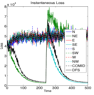
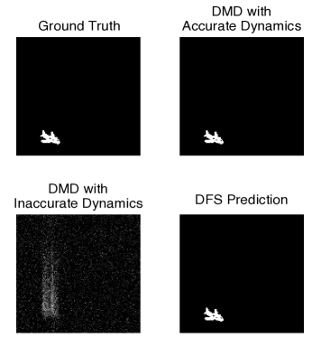
Figures 1 and 2 show the impact of using DFS. We see that DFS switches between dynamical models rapidly and outperforms all of the individual predictions, including COMID, used as a baseline, to show the advantages of incorporating knowledge of the dynamics.

Figure 2: Instantaneous predictions at $t=480$. Top Left: $\theta_{t}$. Top Right: ${\widehat{\theta}}^{(SE)}_{t}$. Bottom Left: ${\widehat{\theta}}_{t}^{(E)}$. Bottom Right: ${\widehat{\theta}}_{t}$. The prediction made with the prevailing motion is an accurate representation of the ground truth, while the prediction with the wrong dynamic is an unclear picture. The DFS algorithm correctly picks out the cleaner picture.

7.2 Tracking dynamic social networks

Dynamical models have a rich history in the context of social network analysis (Snijders, 2001), but we are unaware of their application in the context of online learning algorithms. To show how DMD can bridge this gap, we track the influence matrix of seats in the US Senate from 1795 to 2011 using roll call data (http://www.voteview.com/dwnl.htm). At time $t$, we observe the “yea” or “nay” vote of each Senator, which we represent with a $+1$ or $-1$. When a Senator’s vote is unavailable (for instance, before a state joined the union), we use a $0$. We form a length $p=100$ vector of these votes indexed by the Senate seat, and denote this $x_{t}$.

Following (Ravikumar et al., 2010), we form a loss function using a negative log Ising model pseudolikelihood to sidestep challenging issues associated with the partition function of the Ising model likelihood. For a social network with $p$ agents, $\theta_{t}\in[-1,1]^{p\times p}$, where $(\theta_{t})_{ab}$ corresponds to the correlation in voting patterns between agents $a$ and $b$ at time $t$. Let ${\cal V}$ denote the set of agents, ${\cal V}\backslash a$ the set of all agents except $a$, $x_{a}$ the vote of agent $a$, and $\theta_{a}{\triangleq}\{\theta_{ab}:b\in{\cal V}\}$. Our loss function is

$$\varphi^{(a)}_{t}(\theta_{a}){\triangleq} \log\left[\exp\left(2\theta_{aa}x_{a}+2\textstyle\sum_{b\in{\cal V}\backslash a}\theta_{ab}x_{a}x_{b}\right)+1\right]$$

$$f^{(a)}(\theta_{a};x){\triangleq} -2\theta_{aa}x_{a}-2\textstyle\sum_{b\in{\cal V}\backslash a}\theta_{ab}x_{a}x_{b}+\varphi^{(a)}_{t}(\theta_{a})$$

$$f(\theta;x)= \textstyle\sum_{a\in{\cal V}}f^{(a)}(\theta_{a};x)$$

and $r(\theta)=\tau\|\theta\|_{1}$, where $\tau>0$ is a tuning parameter; this loss is convex in $\theta$. We set $\psi(\theta)=\frac{1}{2}\|\theta\|^{2}_{2}$ and use a dynamical model inspired by (Snijders, 2001), where if $|\theta_{ac^{*}}\theta_{bc^{*}}|>|\theta_{ab}|$, with $c^{*}=\mathop{\!\arg\max}_{c}|\theta_{ac}\theta_{bc}|$, then:

$$(\Phi_{t}^{(i)}(\theta))_{ab}=(1-\alpha_{i})\theta_{ab}+\alpha_{i}\theta_{ac^{*}}\theta_{bc^{*}}.$$

Otherwise, ${\widehat{\theta}}^{(i)}_{ab}={\widetilde{\theta}}^{(i)}_{ab}$. The intuition is that if two members of the network share a strong common connection, they will become connected in time. We set $\alpha_{i}\in\{0,.001,.002,.003,.004\}$ for the different dynamical models. We set $\tau=.1$ and again set $\eta$ using the doubling trick with time horizons at set at increasing powers of 10. As in (Langford et al., 2009), we find that regularizing (e.g., thresholding) every 10 steps, instead of at each time step, allows for the values to grow above the threshold for meaningful relationships to be found.

Figure 3: Tracking a dynamic social network. Losses for different dynamical models and the DFS predictions; $\alpha=0$ corresponds to COMID.

Figure 4: Losses for individual senators. Low losses correspond to predictable, consistent voting behavior, while higher loss means less predictable

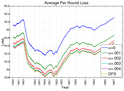
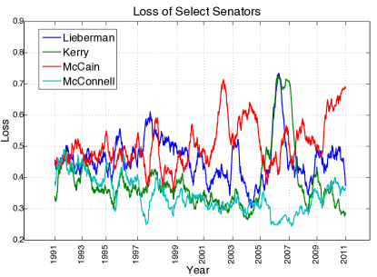
Figure 3 shows the average per round loss of each model, and the DFS estimator over a 30 year time window. We see that applying the dynamical model improves performance relative to COMID ($\alpha_{i}=0$) and that DFS aggregates the predictions successfully. Figure 4 shows the moving average losses for a few Senators, where high loss corresponds to behavior unexpected in the model. Notice that John Kerry (D-MA) has generally low loss, spikes around 2006, and then drops again before a reelection campaign in 2008.

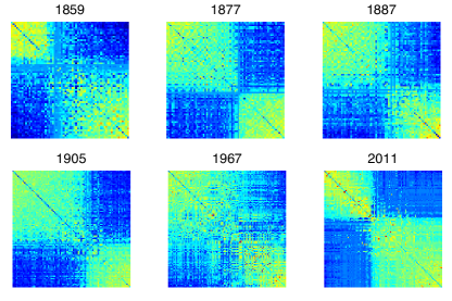
Looking at the network estimates of DFS across time (as in Figure 5) we can see tight factions forming in the mid- to late-1800s (post Civil War), followed by a time when the factions dissipate in the mid-1900s during the Civil Rights Movement. Finally, we see factions again forming in more recent times. The seats are sorted separately for each matrix to emphasize groupings, which align with known political factions.

Figure 5: Influence matrices for select years spanning Civil War and Civil Rights Movement to present, showing formation of factions. Warmer colors (reds and greens) correspond to higher influence and colder (blue) corresponds to lower influence. (Best viewed in color)

8 Conclusion and future directions

In this paper we have proposed a novel online optimization method, called Dynamic Mirror Descent (DMD), which incorporates dynamical model state updates. There is no assumption that there is a “true” known underlying dynamical model, or that the best dynamical model is unchanging with time. The proposed Dynamic Fixed Share (DFS) algorithm adaptively selects the most promising dynamical model from a family of candidates at each time step. Recent work on shifting or tracking regret bounds for online convex optimization further suggest that the techniques developed in this paper may also be useful for bounding adaptive regret or developing methods for automatically tuning step-size parameters (Cesa-Bianchi et al., 2012). In experiments with real and simulated data, DMD shows strong tracking behavior even when underlying dynamical models are switching.

9 Proofs

Proof of Lemma 5:

The optimality condition of (5a) implies

$$\langle\nabla f_{t}( {\widehat{\theta}}_{t})+\nabla r({\widetilde{\theta}}_{t+1}),{\widetilde{\theta}}_{t+1}-\theta_{t}\rangle\leq$$

$$\frac{1}{\eta_{t}}\langle\nabla\psi({\widehat{\theta}}_{t})-\nabla\psi({\widetilde{\theta}}_{t+1}),{\widetilde{\theta}}_{t+1}-\theta_{t}\rangle.$$ (13)

Using this condition we can bound the instantaneous regret as follows:

$$f_{t} ({\widehat{\theta}}_{t})-f_{t}(\theta_{t})+r({\widehat{\theta}}_{t})-r(\theta_{t})$$

$$= f_{t}({\widehat{\theta}}_{t})-f_{t}(\theta_{t})+r({\widehat{\theta}}_{t})-r({\widetilde{\theta}}_{t+1})+r({\widetilde{\theta}}_{t+1})-r(\theta_{t})$$

$$\leq \langle\nabla f_{t}({\widehat{\theta}}_{t}),{\widehat{\theta}}_{t}-\theta_{t}\rangle+\langle\nabla r({\widehat{\theta}}_{t}),{\widehat{\theta}}_{t}-{\widetilde{\theta}}_{t+1}\rangle$$

$$+\langle\nabla r({\widetilde{\theta}}_{t+1}),{\widetilde{\theta}}_{t+1}-\theta_{t}\rangle$$ (14a)

$$\leq \frac{1}{\eta_{t}}\langle\nabla\psi({\widehat{\theta}}_{t})-\nabla\psi({\widetilde{\theta}}_{t+1}),{\widetilde{\theta}}_{t+1}-\theta_{t}\rangle$$

$$+\langle\nabla f_{t}({\widehat{\theta}}_{t})+\nabla r({\widehat{\theta}}_{t}),{\widehat{\theta}}_{t}-{\widetilde{\theta}}_{t+1}\rangle$$ (14b)

$$= \frac{1}{\eta_{t}}\left[D(\theta_{t}\|{\widehat{\theta}}_{t})-D(\theta_{t+1}\|{\widehat{\theta}}_{t+1})\right]$$

$$+T_{3}+T_{4}/\eta_{t}+T_{5}/\eta_{t}\hskip 18.06749pt\text{where,}$$ (14c)

$$T_{3}{\triangleq} -\frac{1}{\eta_{t}}D({\widetilde{\theta}}_{t+1}\|{\widehat{\theta}}_{t})+\langle\nabla\ell_{t}({\widehat{\theta}}_{t}),{\widehat{\theta}}_{t}-{\widetilde{\theta}}_{t+1}\rangle$$

$$T_{4}{\triangleq} \left[D(\Phi_{t}(\theta_{t})\|\Phi_{t}({\widetilde{\theta}}_{t+1}))-D(\theta_{t}\|{\widetilde{\theta}}_{t+1})\right]\leq\Delta_{\Phi_{t}}$$

$$T_{5}{\triangleq} \left[D(\theta_{t+1}\|{\widehat{\theta}}_{t+1})-D(\Phi_{t}(\theta_{t})\|{\widehat{\theta}}_{t+1})\right].$$

Here, (14a) follows from the convexity of $f_{t}$ and $r$, (14b) follows from the optimality condition of (5a), and (14c) follows from (3c) and adding and subtracting terms using the equivalence (5b). Each of term can be bounded, and then combined to complete the proof.

$$T_{3}\leq -\frac{\sigma}{2\eta_{t}}\|{\widetilde{\theta}}_{t+1}-{\widehat{\theta}}_{t}\|^{2}$$

$$+\frac{\sigma}{2\eta_{t}}\|{\widetilde{\theta}}_{t+1}-{\widehat{\theta}}_{t}\|^{2}+\frac{\eta_{t}}{2\sigma}G_{\ell}^{2}=\frac{\eta_{t}}{2\sigma}G_{\ell}^{2}$$ (15a)

$$T_{5}= \psi(\theta_{t+1})-\langle\nabla\psi({\widehat{\theta}}_{t+1}),\theta_{t+1}-{\widehat{\theta}}_{t+1}\rangle$$

$$-\psi(\Phi_{t}(\theta_{t}))+\langle\nabla\psi({\widehat{\theta}}_{t+1}),\Phi_{t}(\theta_{t})-{\widehat{\theta}}_{t+1}\rangle$$

$$= \psi(\theta_{t+1})-\psi(\Phi_{t}(\theta_{t}))-\langle\nabla\psi({\widehat{\theta}}_{t+1}),\theta_{t+1}-\Phi_{t}(\theta_{t})\rangle$$

$$\leq 4M\|\theta_{t+1}-\Phi_{t}(\theta_{t})\|$$ (15b)

where (15a) is due to the strong convexity of the Bregman Divergence and Young’s inequality and (15b) is due to the convexity of $\psi$ and the Cauchy-Schwarz inequality. Combining these inequalities with (14c) gives the Lemma as it is stated. $\Box$

References

- Angelosante et al. (2009) Angelosante, D., Giannakis, G. B., and Grossi, E. Compressed sensing of time-varying signals. In Int’l Conf. on Dig. Sig. Proc., 2009.
- Bain & Crisan (2009) Bain, A. and Crisan, D. Fundamentals of Stochastic Filtering. Springer, 2009.
- Banerjee et al. (2008) Banerjee, O., El Ghaoui, L., and d’Aspremont, A. Model selection through sparse maximum likelihood estimation for multivariate Gaussian or binary data. J. Mach. Learn. Res., 9:485–516, 2008.
- Beck & Teboulle (2003) Beck, A. and Teboulle, M. Mirror descent and nonlinear projected subgradient methods for convex programming. Operations Research Letters, 31:167–175, 2003.
- Belkin & Niyogi (2003) Belkin, M. and Niyogi, P. Laplacian eigenmaps for dimensionality reduction and data representation. Neural Comput., 15(6):1373–1396, June 2003.
- Candès et al. (2006) Candès, E., Romberg, J., and Tao, T. Stable signal recovery from incomplete and inaccurate measurements. Communications on Pure and Applied Mathematics, 59(8):1207–1223, 2006.
- Cesa-Bianchi & Lugosi (2006) Cesa-Bianchi, N. and Lugosi, G. Prediction, Learning and Games. Cambridge University Press, New York, 2006.
- Cesa-Bianchi et al. (2012) Cesa-Bianchi, N., Gaillard, P., Lugosi, G., and Stoltz, G. A new look at shifting regret. arXiv:1202.3323, 2012.
- Duarte et al. (2008) Duarte, M. F., Davenport, M. A., Takhar, D., Laska, J. N., Sun, T., Kelly, K. F., and Baraniuk, R. G. Single pixel imaging via compressive sampling. IEEE Sig. Proc. Mag., 25(2):83–91, 2008.
- Duchi et al. (2010) Duchi, J., Shalev-Shwartz, S., Singer, Y., and Tewari, A. Composite objective mirror descent. In Conf. on Learning Theory (COLT), 2010.
- Gyorgy et al. (2012) Gyorgy, A., Linder, T., and Lugosi, G. Efficient tracking of large classes of experts. IEEE Transaction on Information Theory, 58:6709–6725, November 2012.
- Hazan & Seshadhri (2009) Hazan, E. and Seshadhri, C. Efficient learning algorithms for changing environments. In Proc. Int. Conf on Machine Learning (ICML), pp. 393–400, 2009.
- Herbster & Warmuth (2001) Herbster, M. and Warmuth, M. K. Tracking the best linear predictor. Journal of Machine Learning Research, 35(3):281–309, 2001.
- Kolar et al. (2010) Kolar, M., Song, L., Ahmed, A., and Xing, E. P. Estimating time-varying networks. Annals of Applied Statistics, 4(1):94–123, 2010.
- Langford et al. (2009) Langford, J., Li, L., and Zhang, T. Sparse online learning via truncated gradient. J. Mach. Learn. Res., 10:777–801, 2009.
- Littlestone & Warmuth (1994) Littlestone, N. and Warmuth, M. K. The weighted majority algorithm. Inf. Comput., 108(2):212–261, 1994.
- McMahan (2011) McMahan, B. A unified view of regularized dual averaging and mirror descent with implicit updates. arXiv:1009.3240v2, 2011.
- Merhav & Feder (1998) Merhav, N. and Feder, M. Universal prediction. IEEE Trans. Info. Th., 44(6):2124–2147, October 1998.
- Nemirovsky & Yudin (1983) Nemirovsky, A. S. and Yudin, D. B. Problem complexity and method efficiency in optimization. John Wiley & Sons, New York, 1983.
- Rakhlin & Sridharan (2012) Rakhlin, A. and Sridharan, K. Online learning with predictable sequences. arXiv:1208.3728, 2012.
- Ravikumar et al. (2010) Ravikumar, P., Wainwright, M. J., and Lafferty, J. D. High-dimenstional Ising model selection using -regularized logistic regression. Annals of Statistics, 38:1287–1319, 2010.
- Snijders (2001) Snijders, T. A. B. The statistical evaluation of social network dynamics. Sociological Methodology, 31(1):361–395, 2001.
- Theodor & Shaked (1996) Theodor, Y. and Shaked, U. Robust discrete-time minimum-variance filtering. IEEE Trans. Sig. Proc., 44(2):181–189, 1996.
- Vaswani & Lu (2010) Vaswani, N. and Lu, W. Modified-CS: Modifying compressive sensing for problems with partially known support. IEEE Trans. Sig. Proc., 58:4595–4607, 2010.
- Xiao (2010) Xiao, L. Dual averaging methods for regularized stochastic learning and online optimization. J. Mach. Learn. Res., 11:2543–2596, 2010.
- Xie et al. (1994) Xie, L., Soh, Y. C., and de Souza, C. E. Robust Kalman filtering for uncertain discrete-time systems. IEEE Trans. Autom. Control, 39:1310–1314, 1994.
- Zinkevich (2003) Zinkevich, M. Online convex programming and generalized infinitesimal gradient descent. In Proc. Int. Conf. on Machine Learning (ICML), pp. 928–936, 2003.