Proceedings of CKM 2012, the 7th International Workshop on the CKM Unitarity Triangle, University of Cincinnati, USA, 28 September - 2 October 2012

Search for $B\rightarrow\nu\overline{\nu}$ and related modes with the BABAR detector

Alessandro Rossi, on behalf of BABAR collaboration
Instituto Nazionale di Fisica Nucleare - Sezione di Perugia
06123 Perugia, ITALY

1 Introduction

In the Standard Model (SM), a weak decay such as $B^{0}\rightarrow\nu\overline{\nu}(+\gamma$) can only occur through second-order diagrams like those shown in Fig. 1. All these processes are highly suppressed within the SM.

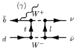
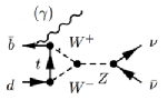
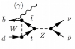
Figure 1: The lowest-order SM Feynman graphs for $B^{0}\rightarrow$ invisible (+ $\gamma$) decays: a) box diagram, b) and c) weak annihilation diagrams.

Like all purely leptonic $B$ decays, they contain a $b\rightarrow d$ transition plus an internal quark annihilation that further suppresses the amplitude with respect to rare semileptonic decays. In addition, helicity suppression factors proportional to $m_{\nu}^{2}$ make the $\nu\overline{\nu}$ channel completely undetectable in the SM scenario. For the $\nu\overline{\nu}\gamma$ channel the latter factor is not present, resulting in SM branching fraction expectations at the $10^{-10}$ level [1]. Several new physics models predict enhancements of these branching ratios up to values close to the experimental detection: a phenomenological model allows for associated neutralino production from $B^{0}$ decays with a branching fraction in the $10^{-7}$ to $10^{-6}$ range [2]. Also, models with large extra dimensions can have the effect of producing significant, although small, rates for invisible $B^{0}$ decays [3, 4, 5].

The data used in this analysis were collected with the BABAR detector at the PEP-II $e^{+}e^{-}$ collider at SLAC. The data sample corresponds to a luminosity of 424 fb^-1 accumulated at the $\mathchar 28935\relax(4S)$ resonance and contains $(471\pm 3)\times 10^{6}$ $B\overline{B}$ pair events. For background studies we also used 45 fb^-1 collected at a center-of-mass (CM) energy about 40 MeV below the $B\overline{B}$ threshold (off peak). A detailed description of the BABAR detector is presented in Ref. [6].

More details on these analysis may be found in Ref. [7].

2 Reconstruction and selection

The detection of invisible $B$ decays uses the fact that $B$ mesons are created in pairs, due to flavor conservation in $e^{+}e^{-}$ interactions. We reconstruct events in which a $\overline{B}^{0}$ decays to $D^{(*)+}\ell^{-}\overline{\nu}$ (referred to as the “tag side”), then look for consistency with an invisible decay or a decay to a single photon of the other neutral $B$ (referred to as the “signal side”).

In the signal event selection we consider events with no charged tracks besides those from the $\overline{B}^{0}\rightarrow D^{(*)+}\ell^{-}\overline{\nu}$ candidate. In order to reject background events where one charged or neutral particle is lost along the beam pipe, the cosine of the polar angle of the missing momentum in the CM frame ($\cos\theta^{*}_{miss}$) is required to lie in the $[-0.9,0.9]$ range.

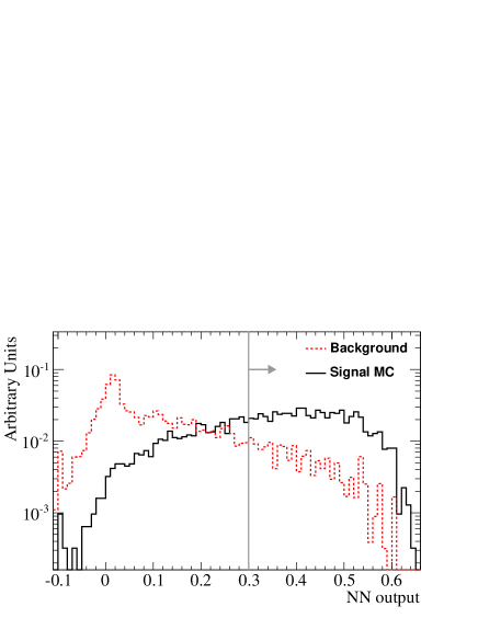
Figure 2: Distributions of the NN output for simulated $B^{0}$ $\rightarrow$ invisible events with a $D$ meson on the tag side. The black solid line is the signal while the red dashed line is the background. The solid gray vertical line defines the NN output signal region.

For the $B^{0}\rightarrow$ invisible decay, in events where the $D$ meson on the tag side decays into $K^{-}\pi^{+}\pi^{-}$, two additional selection criteria are also applied: on the sum of the angles between the Kaon and each one of the two $\pi$s and on the sum of the angles between the lepton and each one of the two $\pi$s. To reconstruct $B^{0}\rightarrow$ invisible$+\gamma$ events, one remaining photon candidate with energy greater than 1.2 $\mathrm{\,Ge\kern-1.00006ptV}$ in the CM frame is also required.

An artificial neural network (NN) is used to provide further discrimination between signal and background events. Events with a $D$ or a $D^{*}$ meson on the tag side are split in two different categories and a different NN was used for each sub-sample. For the $B^{0}\rightarrow$ invisible decay 9 and 6 variables are used for $D$ and $D^{*}$ sub-samples, respectively, while for the $B^{0}\rightarrow$ invisible$+\gamma$ decay we used 6 and 4 variables. These variables are mainly kinematical and refer to the tag side reconstruction. The two most important are the cosine of the angle between the $B$ meson and the $D^{(*)}\ell$ pair, defined as

$$\cos\theta_{B,D^{(*)-}\ell^{+}}=\frac{2\,E_{B}E_{{D^{(*)-}\ell^{+}}}-m^{2}_{{B}}-m^{2}_{{D^{(*)-}\ell^{+}}}}{2\,|\vec{p}_{B}||\vec{p}_{{D^{(*)-}\ell^{+}}}|},$$ (1)

and $M_{miss}^{tag}$ (defined as the invariant mass of the event after the $D^{(*)-}\ell^{+}$ pair is subtracted). In the $B^{0}\rightarrow$ invisible$+\gamma$ analysis, we additionally use the energy of the photon on the signal side, evaluated in the laboratory frame. In Fig. 2, the output of the NN for simulated $B^{0}\rightarrow$ invisible with a $D$ meson on the tag side, and the corresponding signal region, are shown.

After the NN selection, the $D$ meson invariant mass ($m_{D}$) and the difference between the reconstructed $D^{*}$ invariant mass and the PDG $D^{0}$ mass ($\Delta m$) are used to define a

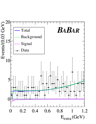
Figure 3: Results of the maximum likelihood fit of $E_{\rm extra}$ for $B^{0}\rightarrow$ invisible (left) and $B^{0}\rightarrow$ invisible$+\gamma$ (right).

signal region and a sideband region for the $D$ tag and $D^{*}$ tag samples, respectively. The signal region is defined as a $\pm$15 ${\mathrm{\,Me\kern-1.00006ptV\!/}c^{2}}$ window around the PDG value for $m_{D}$, and as 0.139 $<\Delta m<$ 0.148 ${\mathrm{\,Ge\kern-1.00006ptV\!/}c^{2}}$. The excluded regions are used as sidebands.

The neutral energy that remains after all tag side tracks and neutral clusters have been accounted for is denoted as $E_{\rm extra}$. For $B^{0}\rightarrow$ invisible$+\gamma$, the energy of the highest-energy photon remaining in the event (the signal photon candidate) is also removed from the $E_{\rm extra}$ computation. The $E_{\rm extra}$ signal region is defined by imposing an upper bound at 1.2 $\mathrm{\,Ge\kern-1.00006ptV}$.

We construct probability density functions (PDFs) for the $E_{\rm extra}$ distribution for signal ($\mathcal{P}_{\rm sig}$) and background ($\mathcal{P}_{\rm bkg}$) using detailed MC simulations for signal and data from the $m_{D}$ and $\Delta m$ sidebands for background. The two PDFs are combined into an extended maximum likelihood function $\mathcal{L}$, defined as a function of the free parameters $N_{\rm sig}$ and $N_{\rm bkg}$, the number of signal and background events, respectively. The photon reconstruction algorithm has a lower cluster energy cut of 30 $\mathrm{\,Me\kern-1.00006ptV}$, and as a consequence, the $E_{\rm extra}$ distribution is not continuous. To account for this effect, the likelihood is composed of two distinct parts, one for $E_{\rm extra}>30$ $\mathrm{\,Me\kern-1.00006ptV}$ and one for $E_{\rm extra}=0$ $\mathrm{\,Me\kern-1.00006ptV}$.

The negative log-likelihood is then minimized with respect to $N_{\rm sig}$ and $N_{\rm bkg}$ in the data sample. The resulting fitted values for $N_{\rm sig}$ and $N_{\rm bkg}$ are given in Table 1. Figure 3 shows the $E_{\rm extra}$ distributions for $B^{0}\rightarrow$ invisible and $B^{0}\rightarrow$ invisible$+\gamma$ with the fit superimposed.

Mode	$N_{\rm sig}$	$N_{\rm bkg}$
$B^{0}\rightarrow$ invisible	$-22\pm 9$	$334\pm 21$
$B^{0}\rightarrow$ invisible$+\gamma$	$-3.1\pm 5.2$	$113\pm 12$

Table 1: Fitted yields of signal and background events in data. The uncertainties are statistical.

Using detailed Monte Carlo simulations of $B^{0}\rightarrow$ invisible and $B^{0}\rightarrow$ invisible$+\gamma$ events, we determine our signal efficiency to be $(17.8\pm 0.2)\times 10^{-4}$ for $B^{0}\rightarrow$ invisible and $(16.0\pm 0.2)\times 10^{-4}$ for $B^{0}\rightarrow$ invisible$+\gamma$, where the uncertainties are statistical.

Source	$B^{0}\rightarrow$ invisible	$B^{0}\rightarrow$ invisible$+\gamma$	Source	$B^{0}\rightarrow$ invisible	$B^{0}\rightarrow$ invisible$+\gamma$
Normalization Errors			Efficiency Errors
$B$-counting	$0.6\%$	$0.6\%$	Tagging Efficiency	$3.5\%$	$3.5\%$
Yield Errors (events)			$m_{D}$ $(\Delta m)$ Selection	$1\%$	$1.3\%$
Background Param.	$15.8$	$6.5$	Preselection	$3\%$	$2.4\%$
Signal Param.	$2.0$	$1.2$	Neural Network	$6.1\%$	$8.2\%$
Fit Technique	–	$1.0$	Single Photon	–	$1.8\%$
$E_{\rm extra}$ Shape	$0.1$	$1.8$	TOTAL	$7.7\%$	$9.5\%$
TOTAL	$15.9$	$6.9$

Table 2: Summary of the systematic uncertainties.

The systematic uncertainty on the signal efficiency is dominated by data-MC discrepancies in the distribution of the variables used as input to the NN while the main systematic uncertainty on the signal yield is dominated by the background parametrization uncertainties. The total systematic uncertainty on the signal selection efficiency is 7.7% for $B^{0}\rightarrow$ invisible decay and 9.5% for $B^{0}\rightarrow$ invisible$+\gamma$ decay and the total systematic errors on the signal yield are 16 and 7 events for $B^{0}\rightarrow$ invisible and $B^{0}\rightarrow$ invisible$+\gamma$, respectively. All systematic uncertainties are summarized in Table 2.

3 Conclusions

A Bayesian approach is used to set 90% confidence level (CL) upper limits on the branching fractions for $B^{0}\rightarrow$ invisible and $B^{0}\rightarrow$ invisible$+\gamma$. Flat prior probabilities are assumed for positive values of both branching fractions. Gaussian likelihoods are adopted for signal yields. The Gaussian widths are fixed to the sum in quadrature of the statistical and systematic yield errors. We extract a posterior PDF using Bayes’ theorem, including in the calculation the effect of systematic uncertainties associated with the efficiencies and the normalizations, modeled by Gaussian PDFs. Given the observed yields in Table 1, the 90% CL upper limits are

$$\mathcal{B}(B^{0}\rightarrow{\rm invisible}) < 2.4\times 10^{-5}$$

$$\mathcal{B}(B^{0}\rightarrow{\rm invisible}+\gamma) < 1.7\times 10^{-5}$$

at 90% CL. These limits supercede our earlier results [8], which used a small fraction of our present dataset, and the recent Belle result [9].

References

- [1] S. Adler et al. (BNL-787 Collaboration), Phys. Rev. Lett. 84, 3768 (2007);
- [2] A. Dedes, H. Dreiner, and P. Richardson, Phys. Rev. D 65, 015001 (2002).
- [3] K. Agashe, N. G. Deshpande, and G.-H. Wu, Phys. Lett. B 489, 367 (2000).
- [4] K. Agashe and G.-H. Wu, Phys. Lett. B 498, 230 (2001).
- [5] H. Davoudiasl, P. Langacker, and M. Perelstein, Phys. Rev. D 65, 105015 (2002).
- [6] B. Aubert et al. (BABAR Collaboration), Nucl. Instrum. Meth. A 479 (2002).
- [7] J. P. Lees et al. (BABAR Collaboration), Phys. Rev. D 86, 051105 (2012).
- [8] B. Aubert et al. (BABARCollaboration), Phys. Rev. Lett. 93, 091802 (2004);
- [9] C. L. Hsu et al. [Belle Collaboration], Phys. Rev. D 86, 032002 (2012).