Modeling high energy cosmic rays mass composition data via mixtures of multivariate skew-t distributions

Abstract

We consider multivariate skew-t distributions for modeling composition data of high energy cosmic rays. The model has been validated with simulated data for different primary nuclei and hadronic models focusing on the depth of maximum $X_{\mathrm{max}}$ and number of muons $N_{\mu}$ observables. Further, we consider mixtures of multivariate skew-t distributions for cosmic ray mass composition determination and event-by-event classification. With respect to other approaches in the field, it is based on analytical calculations and allows to incorporate different sets of constraints provided by the present hadronic models. We present some applications to simulated data sets generated with different nuclear abundances assumptions. As it does not fully rely on the hadronic model predictions, the method is particularly suited to the current experimental scenario in which evidences of discrepancies of the measured data with respect to the models have been reported for some shower observables, such as the number of muons at ground level.

1 Introduction

The nuclear composition of cosmic ray particles is a crucial observable to explore the origin of such radiation at energies above $10^{18}$ eV. Different theoretical models have been advanced in this direction predicting a given flux from each nuclear component. The measurement of the relative abundances as a function of the primary energy at least for groups of nuclear components therefore provide a deep insight in the field and contribute to significantly constrain the present theories.

At energies above the knee the measurement of the mass must necessarily be based on indirect techniques, making use of shower parameters sensitive to the primary mass. Among these, the depth $X_{\mathrm{max}}$ at which the longitudinal development has its maximum and the number of muons $N_{\mu}$ reaching ground level are the most powerful observables. A recent review of the mass composition methods and experimental results over the entire energy spectrum range is presented in [1].
At present, different statistical methods are employed depending on whether the composition information has to be reconstructed on an event-by-event basis. For instance this results to be extremely helpful when studying possible correlations of the shower arrival direction with given astrophysical objects, in proton-Air cross section analysis or in the search of gamma ray or neutrino events in the hadronic background. In all these situations pattern recognition methods, e.g. neural networks as in [2, 3, 4], linear discriminant analysis [5], supervised clustering algorithms as in [4], are typically adopted. To determine the nuclear composition on average, binned likelihood methods, as in [6], or unfolding analyses, as in [7], are preferred.

The presence of stochastic shower-to-shower fluctuations and the experimental resolution currently achieved in the measurement of the shower parameters impose a limit on the number of mass groups to be determined in both kind of analyses, typically less than five.

All these methods directly compare the observed data with mixtures of distributions generated with detailed Monte Carlo simulations of the shower development in atmosphere for each nucleus. The only parameters to be optimized are the component weights.

Shower simulations strongly rely on theoretical models of the hadronic interactions extrapolated at energies well beyond those reached in modern accelerators. Among them we cite Qgsjet01 [8], QgsjetII [9], Sibyll [10] and Epos [11]. Surprisingly, most of the shower observables measured so far at such extreme energies are well described or at least bracketed by the hadronic model predictions, i.e. see [1]. Furthermore, the discrepancies among different models will be significantly reduced with incoming model releases accounting for recent LHC measurements, for instance see [12]. Recently, however, a significant discrepancy between measured data and Monte Carlo simulations has been reported in the muon number estimator both for vertical [13] and for very inclined showers [14]. The origin of such discrepancy is currently under investigation.

This scenario motivates the development of a statistical model of the shower observables and an unsupervised approach, incorporating the valid constraints provided by the hadronic models, for mass composition fitting and classification purposes. These represent the main goals of the present study, which is organized as follows.

In Section 2 we explored the possibility of modeling all shower observables, focusing our attention on the depth of maximum $X_{\mathrm{max}}$ and the number of muons $N_{\mu}$, by using a multivariate skew-t distribution. This and similar classes of skew distributions are receiving a growing attention in model-based clustering over the last few years, i.e. see the works by Lee and Mc Lachlan [15], Vrbik and McNicholas [16], Franczak et al [17] and Azzalini and Genton [18], due to their flexibility to model non-gaussian asymmetric data and the possibility of developing elegant and relatively computationally straightforward mixture solutions in the EM framework. The validation of the model with Monte Carlo shower simulations is reported in paragraph 2.1.
In Section 3.1 we describe the clustering algorithm adopted for composition determination. It is mainly based on the work by McNicholas et al [16] for what concerns the analytical solutions to fit mixtures of multivariate skew-t distributions using the EM algorithm. With respect to the latter work we introduced in Section 3.2 a procedure to account for different kind of constraints in the optimization directly derived from shower simulations. Finally, in Section 4 we applied the method to sample data sets simulated with different nuclear abundance assumptions. The achieved fitting and classification performances are presented and discussed.

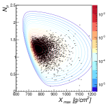
(a) p

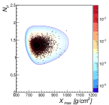
(b) He

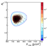
(c) Li

(d) C

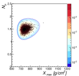
(e) N

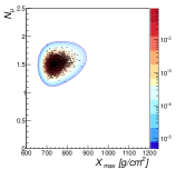
(f) O

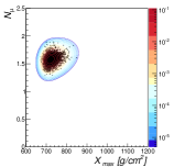
(g) Si

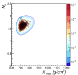
(h) Ca

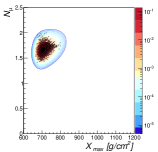
(i) Fe

Figure 1: $X_{\mathrm{max}}$-$N_{\mu}$ distribution for different primary nuclei at $10^{19}$ eV predicted by the Epos1.99 model.

2 Modeling the distribution of cosmic ray shower observables

The fluctuations observed in the shower observables for a given primary nucleus and energy are related to the stocastic fluctuations in the position of the first interaction point in the top layers of the atmosphere and in the secondary interactions occuring along the shower development. The latter can be considered as Gaussian distributed, given the large number of particles involved, while an exponential distribution is assumed for the interaction probability. The resulting distribution is asymmetric with a given degree of skewness depending on the considered parameters. It turns out from these considerations that a suitable distribution describing the fluctuation of a single shower observable $x$ is a convolution of the exponential and gaussian distributions (exponentially modified gaussian (EMG)) [19]:

$$f(x)=\frac{1}{2\lambda}\exp{\left(-\frac{x-\mu}{\lambda}+\frac{\sigma^{2}}{2\lambda^{2}}\right)}\left[1+\operatorname{erf}\left(\frac{x-\mu}{\sigma\sqrt{2}}-\frac{\sigma}{\lambda\sqrt{2}}\right)\right]$$ (2.1)

where $\lambda$ is the attenuation parameter of the exponential function, $\mu$ and $\sigma$ the mean and width parameters of the gaussian function, and $erf$ the standard error function. The above model is based on physical considerations and provides a good representation of both simulated and real data. However, to our knowledge, little efforts have been carried out to describe the joint distribution of several shower observables and no analytical solutions exists to fit a mixture of EMG distributions. For this reason in this work we propose a different model, based on the multivariate skew-t (MST) distribution, to describe the fluctuations of $m$ shower observables $\mathbf{x}$. It is as flexible as model 2.1 in reproducing the skewness observed in the shower observables and, as we will show in section 3.1, it has the great advantage that a closed form exists for mixture fitting with the EM algorithm.

Based on [25, 26, 16], we say that a random vector $\mathbf{X}$ follows a $q$-variate skew-$t$ distribution $f(\mathbf{x};\mbox{\boldmath$\phi$})$ with location vector $\mu$, covariance matrix $\Sigma$, skewness vector $\delta$ and $\nu$ degrees of freedom if it can be represented by

$$\mathbf{X}=\mbox{\boldmath$\delta$}|U|+\mathbf{U}_{0}$$

where $\mathbf{U}_{0}|u,w\sim N_{p}(\mbox{\boldmath$\mu$}+\mbox{\boldmath$\delta$}|u|,\mbox{\boldmath$\Sigma$}/w)$, $U|w\sim N(0,1/w)$ and $W\sim\Gamma(\nu/2,\nu/2)$. The joint distribution of $\mathbf{X},U$ and $W$ is given by:

$$f(\mathbf{x},u,w)=Cw^{R-1}e^{-wS}$$ (2.2)

where $\Gamma(\cdot)$ is the Gamma function and:

$$S= \frac{1}{2}[(\mathbf{x}-\mbox{\boldmath$\mu$}-\mbox{\boldmath$\delta$}|u|)^{T}\mbox{\boldmath$\Sigma$}^{-1}(\mathbf{x}-\mbox{\boldmath$\mu$}-\mbox{\boldmath$\delta$}|u|)+u^{2}+\nu]$$

$$R= (\nu+p+1)/2$$

$$C= (\nu/2)^{\nu/2}\left[(2\pi)^{\frac{p+1}{2}}|\mbox{\boldmath$\Sigma$}|^{1/2}\Gamma(\nu/2)\right]^{-1}\,.$$

Integrating out $u$ and $w$ from the joint distribution we get the expression of the multivariate skew-t distribution:

$$f(\mathbf{x};\mbox{\boldmath$\phi$})=2C\Gamma(R)\frac{D^{\frac{1}{2}-R}}{\sqrt{a}}I_{1}\left(R,\frac{b}{\sqrt{Da}}\right)$$ (2.3)

where:

$$a =\frac{1}{2}(1+\mbox{\boldmath$\delta$}^{\prime}\mbox{\boldmath$\Sigma$}^{-1}\mbox{\boldmath$\delta$})$$

$$b =-\frac{1}{2}(\mathbf{x}-\mbox{\boldmath$\mu$})^{\prime}\mbox{\boldmath$\Sigma$}^{-1}\mbox{\boldmath$\delta$}$$

$$c =\frac{1}{2}(\mathbf{x}-\mbox{\boldmath$\mu$})^{\prime}\mbox{\boldmath$\Sigma$}^{-1}(\mathbf{x}-\mbox{\boldmath$\mu$})+\nu/2$$

$$D =c-b^{2}/a$$

$$I_{1}(E,\alpha)=\int_{\alpha}^{\infty}(1+x^{2})^{-E}dx= \frac{\pi\Gamma(2E-1)}{\Gamma(E)^{2}2^{2E-1}}-\alpha\;_{2}F_{1}\{1/2,E,3/2,-\alpha^{2}\}$$

in which ${}_{2}F_{1}$ denotes the generalized Gauss hypergeometric function, given by:

$${}_{2}F_{1}(x,y;z;1)=\frac{\Gamma(z)\Gamma(z-x-y)}{\Gamma(z-x)\Gamma(z-y)}\,.$$

Finally, $\phi$ denotes the overall parameter of the distribution, that is $\mbox{\boldmath$\phi$}=(\mbox{\boldmath$\mu$},\mbox{\boldmath$\Sigma$},\mbox{\boldmath$\delta$},\nu)$.

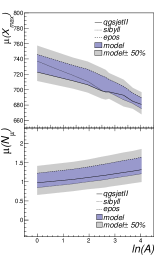
(j) $\mu$ constraints

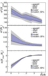
(k) $\Sigma$ constraints

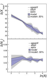
(l) $\delta$ constraints

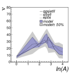
(m) $\nu$ constraints

Figure 2: Constraint region on the MST parameters from hadronic models as a function of the logarithm of the primary mass $A$.

2.1 Model validation

The model presented in the previous section has been validated with shower simulations generated with Conex v2r2.3 tool [20, 21] for three different hadronic models (QgsjetII [9], Sibyll 2.1 [10], Epos 1.99 [11]) and a large set of primary nuclei ($p$, $He$, $C$, $N$, $O$, $Si$, $Ca$, $Fe$). A fixed primary energy was assumed in the simulation, ranging from $10^{17}$ to 10²⁰ eV in step of $\log_{10}E$=0.5, and a zenith range from 0^∘ to 90^∘. We restrict the analysis to the shower depth of maximum $X_{\mathrm{max}}$ and the number of muons $N_{\mu}$ at ground level above 1 GeV which represent the most sensitive observables to the primary composition.
In Fig. 1 we report the distribution of the two parameters obtained from Epos simulations for different primary nuclei at an energy of $10^{19}$ eV. The agreement with the MST model is remarkable. Similar plots are obtained for the other two hadronic models (not shown here). In Fig. 2 the fitted values of the MST parameters are reported for the three hadronic interaction models as a function of the logarithm of the nuclear mass. Although $\mu$ and $\Sigma$ do not directly represent the mean and covariance of the distribution, it is noteworthy to retrieve the expected behavior of the means, decreasing with the mass for $X_{\mathrm{max}}$ and increasing for $N_{\mu}$, and of the variances, decreasing with the nuclear mass. Interestingly, the skewness is found to decrease with the nuclear mass for the depth of maximum variable while assumes nearly constant values for the muon component.

3 A mixture model for mass composition analysis

In this section we describe the mixture model we designed for mass composition analysis. It has been developed in C++ with links to the Root tool [27] for numerical integration routines and to the R statistical tool [29] via the RInside/Rcpp interface [28] for multivariate mathematical functions.

Assume we are provided with a set of $N$ cosmic ray data observations ${\underset{\sim}{\mathbf{X}}}=(\mathbf{x}_{1},\ldots,\mathbf{x}_{N})$ coming from different nuclear species, where $\mathbf{x}_{i}=(X_{\mathrm{max_{i}}},N_{\mu_{\mathrm{i}}})$. In this case, the distribution of the random vector $\mathbf{X}$ can be modeled via a mixture $f(\mathbf{x};\mbox{\boldmath$\theta$})$ of $K$ multivariate skew-$t$ distributions:

$$f(\mathbf{x};\mbox{\boldmath$\theta$})=\sum_{k=1}^{K}\pi_{k}f(\mathbf{x};\mbox{\boldmath$\phi$}_{k})$$ (3.1)

where $\pi_{k}$ are the mixture weights (satisfying $\pi_{k}>0$ and $\sum_{k=1}^{K}\pi_{k}=1$, composition abundances), $f(\mathbf{x};\mbox{\boldmath$\phi$}_{k})$ denotes the density of the $k$ component (2.3) where $\mbox{\boldmath$\phi$}_{k}=(\mbox{\boldmath$\mu$}_{k},\mbox{\boldmath$\Sigma$}_{k},\mbox{\boldmath$\delta$}_{k},\nu_{k})$ denotes the parameters of the $k$th component and $\mbox{\boldmath$\theta$}=\{\mbox{\boldmath$\phi$}_{1},\ldots,\mbox{\boldmath$\phi$}_{k},\pi_{1},\ldots,\pi_{k}\}$ denotes the overall parameter of the mixture.

According to the maximum likelihood approach, the parameters $\theta$ in (3.1) can be estimated by maximizing the log-likelihood function:

$$\log\mathcal{L}(\mbox{\boldmath$\theta$};{\underset{\sim}{\mathbf{X}}})=\log\prod_{i=1}^{N}f(\mathbf{x}_{i};\theta)=\sum_{i=1}^{N}\log f(\mathbf{x}_{i};\theta)\,.$$ (3.2)

The maximization has to be carried out numerically as no analytical solution exists. However it has been shown in [16] that a closed form solution can be obtained using the EM algorithm. In next section we briefly summarize the parameter estimation procedure.

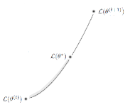
Figure 3: Sketch showing the situation of violating constraints. At iteration (t) constraints are assumed to be satisfied, while at the next iteration (t+1) they are violated. Given the ascent and continuous property of the likelihood in the EM it will exist a point (*) in between the two steps in which the violation occurs. The idea consists of retrieving such point and limit the EM update in the dashed gray region before.

3.1 EM parameter estimation

In the EM framework [24], the $N$ observed data $\mathbf{x}$=($\mathbf{x}_{1}$,…,$\mathbf{x}_{N}$) are considered incomplete and $\mathbf{U}=(u_{1},\ldots,u_{N})$ and $\mathbf{W}=(w_{1},\ldots,w_{N})$ are unobservable latent variables. We introduce the missing data ${\underset{\sim}{\mathbf{Z}}}=(\mathbf{z}_{1},\ldots,\mathbf{z}_{N})$ such that $\mathbf{z}_{i}=(z_{1i},\ldots,z_{Ki})$ (i=1,…N) with $z_{ki}$=1 if $\mathbf{x}_{i}$ comes from the $k$-th component and $z_{ik}$=0 otherwise. The set $({\underset{\sim}{\mathbf{X}}},{\underset{\sim}{\mathbf{Z}}},\mathbf{U},\mathbf{W})$ denotes the complete-data. Thus the complete-data log-likelihood $\mathcal{L}_{c}(\mbox{\boldmath$\theta$})$ can be expressed as:

$$\log\mathcal{L}_{c}(\mbox{\boldmath$\theta$}) =\log\mathcal{L}_{1}(\pi_{1},\ldots,\pi_{K})+\log\mathcal{L}_{2}(\mbox{\boldmath$\mu$}_{1},\mbox{\boldmath$\Sigma$}_{1},\mbox{\boldmath$\delta$}_{1},\ldots,\mbox{\boldmath$\mu$}_{K},\mbox{\boldmath$\Sigma$}_{K},\mbox{\boldmath$\delta$}_{K})+\log\mathcal{L}_{3}(\nu_{1},\ldots,\nu_{K})$$

where

$$\log\mathcal{L}_{1}= \sum_{k=1}^{K}\sum_{i=1}^{N}z_{ki}\log\pi_{k}$$

$$\log\mathcal{L}_{2}= \sum_{k=1}^{K}\sum_{i=1}^{N}\frac{z_{ki}}{2}[\log|\mbox{\boldmath$\Sigma$}_{k}^{-1}|-\log(2\pi)+w_{i}(\mathbf{x}_{i}-\mbox{\boldmath$\mu$}_{k}-\mbox{\boldmath$\delta$}_{k}u_{i})^{T}\mbox{\boldmath$\Sigma$}_{k}^{-1}(bx_{i}-\mbox{\boldmath$\mu$}_{k}-\mbox{\boldmath$\delta$}_{k}u_{i})]$$

$$\log\mathcal{L}_{3}= \sum_{k=1}^{K}\sum_{i=1}^{N}z_{ki}\{-\frac{1}{2}[(p-1)\log w_{i}+w_{i}u_{i}^{2}]+$$

$$\quad+\frac{\nu_{k}}{2}[w_{i}-\log(\nu_{k}/2)]+\log\Gamma(\nu_{k}/2)+(\nu_{k}/2-1)\log w_{i}\}$$

The EM algorithm is first initialized by choosing a starting approximation $\mbox{\boldmath$\theta$}^{(0)}$ for the model parameters and then proceeds by iterating two consecutive steps until convergence. At a given iteration $t$ the $E$ step computes the expected value $Q(\mbox{\boldmath$\theta$}|\mbox{\boldmath$\theta$}^{(t)})$ of the complete log-likelihood, which is maximized in the $M$ step with respect to $\theta$ to obtain a new parameter estimate $\mbox{\boldmath$\theta$}^{(t+1)}$. The following expectations are required to compute $Q(\mbox{\boldmath$\theta$}|\mbox{\boldmath$\theta$}^{(t)})$:

$$\mathbb{E}(Z_{ki}|\mathbf{x}_{i}) =\frac{\pi_{k}^{(t)}f(\mathbf{x}_{i}|\mbox{\boldmath$\theta$}_{k}^{(t)})}{\sum_{k=1}^{K}\pi_{k}^{(t)}f_{k}(\mathbf{x}_{i}|\mbox{\boldmath$\theta$}_{k}^{(t)})}\equiv\tau_{ki}$$

$$\mathbb{E}(Z_{ki}W_{k}|\mathbf{x}_{i}) =P(Z_{ki}=1|\mathbf{x}_{i})\mathbb{E}(W_{k}|x_{i})\equiv P(Z_{ki}=1|\mathbf{x}_{i})e_{1,ki}$$

$$\mathbb{E}(Z_{ki}|U_{k}|W_{k}|\mathbf{x}_{i}) =P(Z_{ki}=1|\mathbf{x}_{i})\mathbb{E}(|U_{k}|W_{k}|\mathbf{x}_{i})\equiv P(Z_{ki}=1|\mathbf{x}_{i})e_{2,ki}$$

$$\mathbb{E}(Z_{ki}U_{k}^{2}W_{k}|\mathbf{x}_{i}) =P(Z_{ki}=1|\mathbf{x}_{i})\mathbb{E}(U_{k}^{2}W_{k}|\mathbf{x}_{i})\equiv P(Z_{ki}=1|\mathbf{x}_{i})e_{3,ki}$$

$$\mathbb{E}(Z_{ki}\log W_{k}|\mathbf{x}_{i}) =P(Z_{ki}=1|\mathbf{x}_{i})\mathbb{E}(\log W_{k}|\mathbf{x}_{i})\equiv P(Z_{ki}=1|\mathbf{x}_{i})e_{4,ki}$$

An analytical calculation of the above expectation terms $e_{1,ki}$, $e_{2,ki}$, $e_{3,ki}$, $e_{4,ki}$ has been recently provided in [16]. Maximizing $Q(\mbox{\boldmath$\theta$}|\mbox{\boldmath$\theta$}^{(t)})$, i.e. setting the derivatives with respect to $\theta$ equal to zero, yields the update estimates of the model parameters at the $t+1$ iteration:

$$\footnotesize\pi_{k}^{(t+1)}= \frac{\sum_{i=1}^{N}\tau_{ki}^{(t)}}{N}$$

$$\mu_{k}^{(t+1)}= \frac{\sum_{i=1}^{N}\tau_{ki}^{(t)}(\mathbf{x}_{i}e_{1,ki}^{(t)}-\delta_{k}e_{2,ki}^{(t)})}{\sum_{i=1}^{N}\tau_{ki}^{(t)}e_{1,ik}^{(t)}}$$

$$\Sigma_{k}^{(t+1)}= \frac{1}{\sum_{i=1}^{N}\tau_{ki}^{(t)}}\{\sum_{i=1}^{N}\tau_{ki}^{(t)}[(\mathbf{x}_{i}-\mbox{\boldmath$\mu$}_{k}^{(t)})(\mathbf{x}_{i}-\mbox{\boldmath$\mu$}_{k}^{(t)})^{T}e_{1,ik}^{(t)}-$$

$$-e_{2,ik}^{(t)}\delta_{k}^{(t)}(\mathbf{x}_{i}-\mbox{\boldmath$\mu$}_{k}^{(t)})^{T}-(\mathbf{x}_{i}-\mbox{\boldmath$\mu$}_{k}^{(t)})\delta_{k}^{(t)}e_{2,ik}^{(t)}+$$

$$+e_{3,ki}^{(t)}\delta_{k}^{(t)}\delta_{k}^{(t)T}\}$$

$$\delta_{k}^{(t+1)}= \frac{\sum_{i=1}^{N}\tau_{ki}^{(t)}e_{2,ki}^{(t)}(\mathbf{x}_{i}-\mbox{\boldmath$\mu$}_{k}^{(t)})}{\sum_{i=1}^{N}\tau_{ki}^{(t)}e_{3,ki}^{(t)}}$$

$$(\log(\nu_{k}^{(t+1)}/2) -\psi(\nu_{k}^{(t+1)}/2)+1)\sum_{i=1}^{N}\tau_{ki}^{(t)}+\sum_{i=1}^{N}\tau_{ki}^{(t)}(e_{4,ki}^{(t)}-e_{1,ki}^{(t)})$$

The $\nu$ update does not exist in closed form and have to be either estimated by solving numerically the above equation or specified in advance. The above update rules guarantee a monotonic increase of the log-likelihood.

3.2 EM constrained

In the case of the mass composition identification of cosmic rays a set of parameter constraints can be derived from physical considerations as well as from predictions obtained with the Heitler model [22, 23] or with the current hadronic models. We report in Fig. 2 the mean $\mu$, covariance matrix $\Sigma$, skewness $\delta$ and degree of freedom $\nu$ parameters as a function of the logarithm of the nuclear mass $\ln(A)$ at an energy of 10¹⁹ eV. The numerical values are obtained by fitting a single MST distribution to our simulated samples. The three black lines correspond to three different hadronic models, the purple area to the region constrained by the three models. As one can see, hadronic models provide stringent lower and upper bounds on the mixture parameters. If we therefore specify in advance the primary masses $A_{k}$ of the mixture groups to be determined from data and order them according to their primary mass ($A_{k}<A_{k+1}$) we can define the following sets of constraints holding for all shower observables:

• Mean constraints: $a_{\mu_{kj}}\leq\mu_{kj}-\mu_{(k+1)j}\leq b_{\mu_{kj}}$, $\forall k$, $j$=1,…,$q$ where $\mu_{kj}$ denotes the $j$th component of the mean vector $\mbox{\boldmath$\mu$}_{k}$, for suitable constants $a_{\mu_{kj}}$, $b_{\mu_{kj}}$.
  As a consequence of the higher interaction cross section of heavy nuclei with the air molecules with respect to light ones, an ordering constraint of the kind $\mu_{j}^{k}\lessgtr\mu_{j}^{k+1}$ is established among each nuclear component means at the same primary energy, e.g. $\mu_{X_{\mathrm{max}}}^{k}<\mu_{X_{\mathrm{max}}}^{k+1}$ or $\mu_{N_{\mu}}^{k}>\mu_{N_{\mu}}^{k+1}$ and so on for other observables. A more stringent constraint, requiring the difference of each component means within a given bound [$a_{\mu_{j}}^{k}$,$b_{\mu_{j}}^{k}$], is provided by the hadronic models.

• Variance constraints: $\sigma_{kjj}>\sigma_{(k+1)jj}$, $a_{\sigma_{kjj}}\leq\sigma_{kjj}\leq b_{\sigma_{kjj}}$ $\forall k$, $j$=1,…,$q$ where $\sigma_{kjj}$ denotes the $j$th diagonal component of the covariance matrix $\mbox{\boldmath$\Sigma$}_{k}$, for suitable constants $a_{\sigma_{kjj}}$, $b_{\sigma_{kjj}}$.
  Due to the larger number of nucleons involved in the interactions, heavy nuclei exhibit smaller shower-to-shower fluctuations in all shower observables compared to light nuclei at the same primary energy, e.g. $\sigma_{X_{\mathrm{max}}}^{k}<\sigma_{X_{\mathrm{max}}}^{k+1}$ and $\sigma_{N_{\mu}}^{k}<\sigma_{N_{\mu}}^{k+1}$. Moreover, hadronic models provides also a constraint bound [$a_{\sigma_{kj}}$,$b_{\sigma_{kj}}$] for each mixture component.

• Skewness and degrees of freedom constraints: $a_{\delta_{kj}}\leq\delta_{kj}\leq b_{\delta_{kj}}$, $a_{\nu_{k}}\leq\nu_{k}\leq b_{\nu_{k}}$ $\forall k$, $j$=1,…,$q$ where $\delta_{kj}$ denotes the $j$th component of the skewness vector $\mbox{\boldmath$\delta$}_{k}$, with $a_{\delta_{kj}}$, $b_{\delta_{kj}}$, $a_{\nu_{kj}}$, $b_{\nu_{kj}}$ constants.
  Useful bound regions on the skewness parameters $\delta$ and $\nu$ are provided by the hadronic models.

When analyzing simulated or real data a larger tolerance region with respect to that defined by the models should be considered for several reasons. First we need to account for possible discrepancies of the data with respect to model predictions. Moreover, if we consider the non-null experimental resolution achieved in the measurement of the shower observables and that the nuclear species are not considered alone in analysis but instead grouped in few general groups (i.e. light-$A$, intermediate-$A$ and heavy-$A$) the variance to be considered for each group $k$ is effectively larger. In Fig. 2 the tolerance region is represented by the gray area defined assuming a $\pm$50% bound with respect to the model constraint region. To incorporate the above constraints in the parameter space of the statistical model we consider the case of a given parameter $\mathbf{\theta}$ violating its constraints at a given iteration $t+1$. At the previous iteration the constraints are assumed to be satisfied. This situation is sketched in Fig. 3. Due to the the continuous and monotonic properties of the likelihood function in the EM we can trace back the exact point $\mathbf{\theta}^{*}$ in which the constraint is violated after the $(t+1)$ update by introducing the following notation:

$$\mathbf{\theta}^{*}=(1-\alpha)\mathbf{\theta}^{(t)}+\alpha\mathbf{\theta}^{(t+1)}$$ (3.3)

with $\alpha$ real values in the range [0,1]. When $\alpha$=0 the parameter estimated at iteration $t$ is obtained, while the update at iteration $t+1$ is obtained when $\alpha$=1. The constraint violation occurs at an intermediate value $\alpha$=$\alpha^{*}$. We note that when $\mathbf{\theta}^{(t+1)}$ satisfies the constraints $\mathbf{\theta}^{*}$ satisfies the constraints $\forall\alpha$. To effectively constrain the EM update it is sufficient to choose an arbitrary $\alpha<\alpha^{*}$, e.g. $\alpha^{*}$/$s$ ($s>1$). In practice we are slowing down the EM algorithm with $s$ controlling the slow-down rate. For the different types of constraints discussed above we have:

• Mean constraint:
  $\alpha^{*}=\underset{j,k}{\min}\left\{\frac{(\mu_{(k+1)j}^{(t)}-\mu_{kj}^{(t)})+a_{\mu_{kj}}}{(\mu_{(k+1)j}^{(t)}-\mu_{kj}^{(t)})-(\mu_{(k+1)j}^{(t+1)}-\mu_{kj}^{(t+1)})}\right\}$, $\alpha^{*}=\underset{j,k}{\min}\left\{\frac{(\mu_{(k+1)j}^{(t)}-\mu_{kj}^{(t)})+b_{\mu_{kj}}}{(\mu_{(k+1)j}^{(t)}-\mu_{kj}^{(t)})-(\mu_{(k+1)j}^{(t+1)}-\mu_{kj}^{(t+1)})}\right\}$

• Variance constraint:
  $\alpha^{*}=\underset{j,k}{\min}\left\{\left[1-\frac{\sigma_{(k+1)jj}^{(t+1)}-\sigma_{kjj}^{(t+1)}}{\sigma_{(k+1)jj}^{(t)}-\sigma_{kjj}^{(t)}}\right]^{-1}\right\}$
  

  $\alpha^{*}=\underset{j}{\min}\left\{\frac{a_{\sigma_{kjj}}-\sigma_{kjj}^{(t)}}{\sigma_{kjj}^{(t+1)}-\sigma_{kjj}^{(t)}}\right\}$, $\alpha^{*}=\underset{j}{\min}\left\{\frac{b_{\sigma_{kjj}}-\sigma_{kjj}^{(t)}}{\sigma_{kjj}^{(t+1)}-\sigma_{kjj}^{(t)}}\right\}$    $\forall k$

• Skewness constraint:
  $\alpha^{*}=\underset{j}{\min}\left\{\frac{a_{\delta_{kj}}-\delta_{kj}^{(t)}}{\delta_{kj}^{(t+1)}-\delta_{kj}^{(t)}}\right\}$, $\alpha^{*}=\underset{j}{\min}\left\{\frac{b_{\delta_{kj}}-\delta_{kj}^{(t)}}{\delta_{kj}^{(t+1)}-\delta_{kj}^{(t)}}\right\}$    $\forall k$

• Degrees of freedom constraint:
  $\alpha^{*}=\left(\frac{a_{\nu_{k}}-\nu_{k}^{(t)}}{\nu_{k}^{(t+1)}-\nu_{k}^{(t)}}\right)$, $\alpha^{*}=\left(\frac{b_{\nu_{k}}-\nu_{k}^{(t)}}{\nu_{k}^{(t+1)}-\nu_{k}^{(t)}}\right)$    $\forall k$

4 Method application to data

In this section we report the fit results (parameter estimation accuracy and classification performances) obtained over random sets ($N_{samples}$=100) of simulated data, generated with the Epos 1.99 model for a reference energy of 10¹⁹ eV. Two kind of samples have been produced with the following specifications:

• Set I: 1000 two-dimensional observations of 3 nuclei ($p$, $N$, $Fe$) with relative abundances set to 0.5, 0.2, 0.3 respectively.

• Set II: 1000 two-dimensional observations of 5 nuclei ($p$, $He$, $N$, $Si$, $Fe$) with relative abundances set to 0.4, 0.1, 0.1, 0.1, 0.3 respectively. Each observation has been convoluted with a gaussian distribution of width $\sigma_{det}$ to take into account the effect of a non-zero experimental resolution. We assumed realistic resolutions for the two variables, namely $\sigma_{det}(X_{\mathrm{max}})$= 20 g/cm² and a comparable resolution for the number of muons $\sigma_{det}(N_{\mu})$= 3%.

The fit of the data are repeated in three different conditions. In a first case we assume that the hadronic models are giving a reasonable representation of the data, hence we fixed all mixture parameters and determine the component fractions. This case, denoted as $\pi$ fit in the following, corresponds to what has been typically done so far when analyzing real cosmic ray data. In a second case, denoted as $(\pi+\mu)$ fit, we assume that the models are not “trustable” in the mean parameters while continue to provide a reasonable description of the data for what concerns the shape of the shower observable distributions. This situation presumably corresponds to what has been recently observed in real data for the muon number observable. We therefore fitted the means and component weights and leave the other parameters fixed. Finally in the third case, denoted as $(\pi+\mu+\Sigma+\delta)$ fit, we released all parameters in the fit but the number of degrees of freedom which is specified in advance.

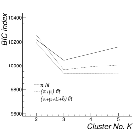
(n) Data Set I

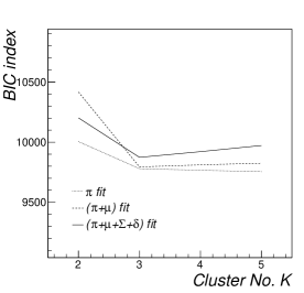
(o) Data Set II

Figure 4: BIC index computed for data sample I (left panel) and II (right panel) as a function of the number of components $K$ for the three fitting assumptions: $\pi$ fit (dotted lines), $\pi$+$\mu$ (dashed lines), $\pi$+$\mu$+$\Sigma$+$\delta$ fit (solid lines).

The parameters are initialized with multiple random starting values ($\sim$100) generated in the constrained space. The best starting values in terms of the maximum log-likelihood achieved are then used for the final fit estimate.
Each optimization is considered to have converged if at a given iteration stage it satisfies the Aitken criterion [30], namely when $\mathcal{L}_{\infty}^{(t+1)}$-$\mathcal{L}^{(t+1)}<\epsilon$ ($\epsilon$=10^-6), where $\mathcal{L}^{(t+1)}$ is the log-likelihood at iteration $t+1$ and $\mathcal{L}_{\infty}^{(t+1)}$ is the asymptotic log-likelihood at iteration $t+1$ [31]:

$$\mathcal{L}_{\infty}^{(t+1)}=\mathcal{L}^{(t)}+\frac{\mathcal{L}^{(t+1)}-\mathcal{L}^{(t)}}{1-a^{(t)}}\;\;\;\;$$ (4.1)

with $a^{(t)}=(\mathcal{L}^{(t+1)}-\mathcal{L}^{(t)})/(\mathcal{L}^{(t)}-\mathcal{L}^{(t-1)})$ Aitken acceleration at iteration $t$.

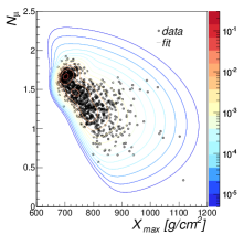
(p) Fit - Data Set I

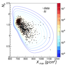
(q) Fit - Data Set II

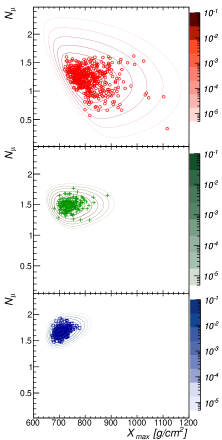
(r) Fit components - Data Set I

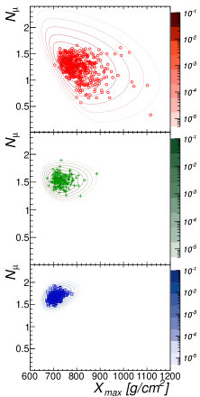
(s) Fit components - Data Set II

Figure 5: Fit results for a data sample generated from set I (left panel) and II (right panel) for the full fit ($\pi$+$\mu$+$\Sigma$+$\delta$) assumption. Top panels: Contour plots of the 3-component MST mixture model fitted to data (empty black dots); Bottom panels: Contour plots of each fitted MST component (red=$p$, green=$N$, blue=$Fe$). Colored dots indicate the true observations from each mass group (see text).

4.1 Choice of the number of components

Several criteria are available in literature to estimate the number of clusters in the data. However, none of these generally leads to definite results, i.e. on the same data set different criteria can predict a different number of optimal clusters, and a user decision is anyway required according to the particular requirements of the analysis. In our case the goal is to provide a best fit of the data with the minimum number of components and the best performances, in terms of classification and mass abundance reconstruction, at least for the light-heavy groups or eventually for three category groups (light-intermediate-heavy).
It is however instructive to test at least one of the available criteria on the market to our problem, for example the Bayesian Information Criterion (bic). The bic index is defined as the maximized value of the likelihood $\log\hat{\mathcal{L}}$ plus a penalty term accounting for possible overfitting of the data as the number of components (model parameters) increases:

$$\mbox{{bic}}=-2\log\hat{\mathcal{L}}+k\log N$$ (4.2)

where $k$ the number of degrees of freedom of the model, e.g. the number of free parameters, and $N$ the number of observations. According to this definition, the model with the larger bic value is the one to be preferred. We report in Fig. 4 the BIC index computed for data sample I (left panel) and II (right panel) for the three fitting assumptions, respectively reported with dotted, dashed and solid lines. As one can see, the criterion effectively manages to predict the real number of components present in the first data sample. Further, it clearly evidences that both data samples cannot be efficiently described with a 2-component model and that 3 components are sufficient to provide an accurate description of data generated by a larger number of components, as in the second data set. We will therefore report in next section the fitting results relative to a 3 component fit.

	$\mathbf{\pi}$ Fit			($\mathbf{\pi}$+$\mathbf{\mu}$) Fit			($\mathbf{\pi}$+$\mathbf{\mu}$+$\mathbf{\Sigma}$+$\mathbf{\delta}$) Fit
Par	Component			Component			Component
$\pi$	0.51	0.19	0.30	0.50	0.20	0.30	0.50	0.22	0.28
$\mu_{1}$	745.86	716.13	689.51	751.11	715.39	689.71	751.38	709.23	688.96
$\mu_{2}$	1.23	1.47	1.65	1.23	1.45	1.64	1.22	1.46	1.65
$\sigma_{11}$	310.56	175.88	90.19	310.56	175.88	90.19	518.71	237.59	84.18
$\sigma_{22}$	0.027	0.0066	0.0047	0.027	0.0066	0.0047	0.032	0.0064	0.0044
$\sigma_{12}$	-2.19	0.03	0.08	-2.19	0.03	0.08	-3.47	-0.52	0.17
$\delta_{1}$	69.84	33.38	23.09	69.84	33.38	23.09	66.15	41.78	24.42
$\delta_{2}$	0.01	0.03	0.03	0.01	0.03	0.03	0.02	0.03	0.03
$\nu$	6.23	27.07	20.46	6.23	27.07	20.46	6.23	27.07	20.46
$\mathcal{L}$	-4964.39			-4487.93			-4947.89
$\varepsilon_{tot}$	0.92			0.91			0.91
$\varepsilon$	0.93	0.82	0.97	0.91	0.81	0.97	0.90	0.87	0.94

Table 1: Fit results for data set I

	$\mathbf{\pi}$ Fit			($\mathbf{\pi}$+$\mathbf{\mu}$) Fit			($\mathbf{\pi}$+$\mathbf{\mu}$+$\mathbf{\Sigma}$+$\mathbf{\delta}$) Fit
Par	Component			Component			Component
$\pi$	0.47	0.20	0.34	0.49	0.18	0.33	0.53	0.18	0.29
$\mu_{1}$	745.86	716.13	689.51	743.79	710.56	690.34	741.39	703.41	691.91
$\mu_{2}$	1.23	1.47	1.65	1.25	1.48	1.64	1.28	1.50	1.65
$\sigma_{11}$	310.56	175.88	90.19	310.56	175.88	90.19	518.71	209.70	113.42
$\sigma_{22}$	0.027	0.0066	0.0047	0.027	0.0066	0.0047	0.033	0.0066	0.0046
$\sigma_{12}$	-2.19	0.03	0.08	-2.19	0.03	0.08	-3.43	-0.45	0.17
$\delta_{1}$	69.84	33.38	23.09	69.84	33.38	23.09	64.27	37.27	21.08
$\delta_{2}$	0.01	0.03	0.03	0.01	0.03	0.03	-0.001	0.03	0.03
$\nu$	6.23	27.07	20.46	6.23	27.07	20.46	6.23	27.07	20.46
$\mathcal{L}$	-4886.3			-4881.5			-4870.27
$\varepsilon_{tot}$	0.86			0.88			0.87
$\varepsilon$	0.87	0.66	0.97	0.92	0.65	0.97	0.94	0.64	0.93

Table 2: Fit results for data set II

4.2 Fitting performances

In Fig. 5 we report the results obtained by fitting a 3-components MST mixture model ($p$+$N$+$Fe$) to one particular sample generated from data set I (left panels) and data set II (right panels). For simplicity we present the results relative to the full fit situation, as the fit results obtained with the other two assumptions are visually similar, and report the values of the fitted parameters with the three fitting assumptions in Tables 1 and 2. The colored lines represent the contour plots of the fitted model. We consider 3 general groups to be fitted: light (1$\leq$A$\leq$4), intermediate (12$\leq$A$\leq$28) and heavy (28$<$A$\leq$56). Lower panels show separately the three groups present in the data with the fitted components superimposed (light: red lines, intermediate: green, heavy: blue). As can be seen in both cases the fit nicely converges towards the expected solution defined by fitting a single MST model to each component alone.
To evaluate the performances achieved for composition reconstruction we report in Figures 3(a) and 3(c) the values of the fitted fractions averaged over the $N_{samples}$ generated samples for three mass groups and fitting conditions ($\pi$ fit: filled dots, $\pi$+$\mu$ fit: empty dots, $\pi$+$\mu$+$\Sigma$+$\delta$ fit: empty squares). The histograms shown with solid lines indicate the true composition fractions. The error bars refer to the obtained fraction RMS. For both data sets the method is able to resolve with good accuracy the three mass groups, with a slightly larger deviation for data set II with respect to the expected values, due to the helium and silicon contamination. Such small bias is however within the uncertainties of the method, found of the order of 0.05 on the reconstructed fractions.

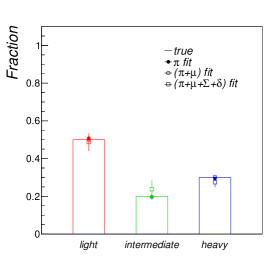
(a) Composition Fit - Data Set I

(b) Classification - Data Set I

(c) Composition Fit - Data Set II

(d) Classification Fit - Data Set II

Figure 6: Performance of composition abundance reconstruction and classification for data set I (upper panels) and II (bottom panels) for the three fitting conditions ($\pi$ fit: filled dots, ($\pi$+$\mu$) fit: empty dots, ($\pi$+$\mu$+$\Sigma$+$\delta$) fit: empty squares) and 3-component groups (light: red, intermediate: green, heavy: blue).

4.3 Classification performances

The fitted model can be used also for classification scopes. Each observation $i$ is assigned to the mixture component $k$ according to the maximum a posteriori probability $\tau_{ik}$. We can therefore compute for both data sets the efficiency $\varepsilon$ achieved for classification. We consider here, as above, the same 3 groups to be identified: light (1$\leq$A$\leq$4), intermediate (12$\leq$A$\leq$28) and heavy (28$<$A$\leq$56). In Tables 1 and 2 we reported the results for each mixture component separately in the case of the data sample analyzed in previous paragraph.
The average classification performances achieved in both data sets are reported in Figures 3(b) and 3(d) for the three groups (light: red, intermediate: green, heavy: blue). In data set I an overall classification efficiency $\varepsilon\sim$0.9 is observed for all fitting cases with a slightly larger error rate for the intermediate component ($\sim$20%). In data set II we have a considerably larger contamination coming from other species with respect to that used to fit the data and hence the event-by-event classification performances are significantly deteriorated for the intermediate component, with typical error rates of $\sim$40%. However, focusing on the two extreme mass groups to be determined, we still manage to achieve a good classification with efficiencies around 90%.
The obtained misclassification errors are comparable with typical results obtained with completely supervised methods, such as neural networks, in [4].

5 Summary

In the present paper we proposed a new model, based on the multivariate skew-$t$ function, to describe the joint distribution of cosmic ray shower observables at high energies. We have tested our model with simulated data for a large set of nuclei, focusing the attention on the depth of shower maximum and number of muons variables, which are the most discriminating in composition studies. We also developed a constrained clustering algorithm to reconstruct the mass composition information of the data, on an event-by-event basis as well as on average (relative abundances). That is a very complicated task given the limited sensitivity of the shower observables to the primary mass and the strong group superposition due to shower-to-shower fluctuations. The designed algorithm allows to include different types of constraints coming from the hadronic model predictions.
We tested the algorithm over samples of data generated with different relative abundances. In the ideal case of perfect measurement precision and negligible contaminations from other species with respect to that used to fit the data we achieved good classification performances, with error rates around 10%, comparable to that found with supervised methods (i.e. neural networks) in [4]. Component abundances and means can be reconstructed with good accuracy too.
The classification performances drop off considerably in a more complicated situation in which a significant contamination from other nuclear species is present together with additive data fluctuations due to the experimental resolution. In this situation the discrimination of the data into three general groups (light-intermediate-heavy) is still feasible, with typical accuracy in the relative abundances $\sim$0.05 depending on the degree of group contaminations.
The algorithm, as it is, can be applied to more than two shower observables (i.e. signal rise time or asymmetries, muon production depth, …) in a very straightforward way. The application to real cosmic ray data is easily done to, as we demonstrated in the case of data sample II, eventually explicitly including the effect of the real experimental resolution in the Monte Carlo templates and simplifying the model by ignoring the correlations relative to variables measured with different detectors.

References

- [1] K.H. Kampert and M. Unger, Measurements of the cosmic ray composition with air shower experiments, Astroparticle Physics 35 (2012) 660.
- [2] A.K.O. Tiba, G.A. Medina-Tanco, S.J. Sciutto, Neural Networks as a Composition Diagnostic for Ultra-high Energy Cosmic Rays, 2005 [arXiv:astro-ph/0502255].
- [3] M.Ambrosio et al, Comparison between methods for the determination of the primary cosmic ray mass composition from the longitudinal profile of atmospheric cascades, Astroparticle Physics 24 (2005) 355.
- [4] S. Riggi et al, Identification of the primary mass of inclined cosmic ray showers from depth of maximum and number of muons parameters, (2012) [arXiv:1212.0218]
- [5] P. Abreu et al, Search for ultrahigh energy neutrinos in highly inclined events at the Pierre Auger Observatory, Physical Review D 84 (2011) 122005.
- [6] D. D’Urso for the Pierre Auger Collaboration, A Monte Carlo exploration of methods to determine the UHECR composition with the Pierre Auger Observatory, in Proc. of 31st International Cosmic Ray Conference (2009) [arXiv:0906.2319].
- [7] T. Antoni at al, KASCADE measurements of energy spectra for elemental groups of cosmic rays: Results and open problems, Astroparticle Physics 24 (2005) 1; W.D. Apel et al, Energy spectra of elemental groups of cosmic rays: Update on the KASCADE unfolding analysis, Astroparticle Physics 31 (2009) 86.
- [8] N.N. Kalmykov et al, Quark-gluon-string model and EAS simulation problems at ultra-high energies, Nucl. Phys. B Proc. Suppl. 52 (1997) 17.
- [9] S. Ostapchenko, Nonlinear screening effects in high energy hadronic interactions, Phys. Rev. D 74 (2006), 014026.
- [10] R.S. Fletcher et al, SIBYLL: An event generator for simulation of high energy cosmic ray cascades, Phys. Rev. D 50 (1994) 5710; J.Engel et al, Nucleus-nucleus collisions and interpretation of cosmic-ray cascades, Phys. Rev. D 46 (1992) 5013.
- [11] K. Werner, The hadronic interaction model EPOS, Nucl. Phys. B Proc. Suppl. 175-176 (2008) 81.
- [12] T. Pierog, LHC results and High Energy Cosmic Ray Interaction Models, in Proc. of 23rd European Cosmic Ray Symposium (2012).
- [13] J. Allen for the Pierre Auger Collaboration, Interpretation of the signals produced by showers from cosmic rays of 1019 eV observed in the surface detectors of the Pierre Auger Observatory, in Proc. of 32nd International Cosmic Ray Conference (2011).
- [14] G. Rodriguez for the Pierre Auger Collaboration, Reconstruction of inclined showers at the Pierre Auger Observatory: implications for the muon content, in Proc. of 32nd International Cosmic Ray Conference (2011).
- [15] S. Lee and G.J. McLachlan, On the fitting of mixtures of multivariate skew t-distributions via the EM algorithm, (2012) [arXiv:1109.4706].
- [16] I. Vrbik, P.D. McNicholas, Analytic calculations for the EM algorithm for multivariate skew-t mixture models, Stat. and Prob. Letters 82 (2012) 1169.
- [17] B.C. Franczak, R.P. Browne and P.D. McNicholas, Mixtures of Shifted Asymmetric Laplace Distributions, (2012) [arXiv:1207.1727]
- [18] A. Azzalini and M.G. Genton, Robust likelihood methods based on the skew-t and related distributions, International Statistical Review 76 (2008) 106.
- [19] R. Ulrich, Introduction to cross section measurements using extensive air showers, in Proceeding of the 12th International Conference on Elastic and Diffractive Scattering (2007).
- [20] T. Pierog et al, First results of fast one-dimensional hybrid simulation of EAS using CONEX, Nucl. Phys. B Proc. Suppl. 151 (2006) 159.
- [21] N.N. Kalmykov et al, One-dimensional hybrid approach to extensive air shower simulation, Astroparticle Physics 26 (2007) 420.
- [22] W. Heitler, The Quantum Theory of Radiation, third ed., Oxford University Press, London, 1954, p. 386.
- [23] J. Matthews, A Heitler model of extensive air showers, Astroparticle Physics 22 (2005) 387.
- [24] A.P. Dempster, A.P., N.M. Laird, D.B. Rubin, Maximum Likelihood from Incomplete Data via the EM Algorithm, Journal of the Royal Statistical Society Series B, 39 (1997) 1.
- [25] S. Pyne et al, Automated high-dimensional flow cytometric data analysis, Proceedings of the National Academy of Sciences 106 (2009) 8519.
- [26] K. Wang et al, Handling Significant Scale Difference for Object Retrieval in a Supermarket, in Proceedings of Conference of Digital Image Computing: Techniques and Applications. IEEE Computer Society, Los Alamitos, California (2009) 526.
- [27] R. Brun and F. Rademakers, Proceedings AIHENP’96 Workshop, Lausanne, Sep. 1996, Nucl. Instr. and Meth. A 389 (1997) 81. See also http://root.cern.ch/
- [28] D. Eddelbuettel and R. François, Journal of Statistical Software 40 (2011) 1.
- [29] R Core Team (2012). R: A language and environment for statistical computing. R Foundation for Statistical Computing, Vienna, Austria. ISBN 3-900051-07-0, URL http://www.R-project.org/.
- [30] A.C. Aitken, On Bernoulli’s numerical solution of algebraic equations, Proceedings of the Royal Society of Edinburgh 46 (1926) 289.
- [31] D. Böhning et al, The distribution of the likelihood ratio for mixtures of densities from the one-parameter exponential family, Annals of the Institute of Statistical Mathematics 46 (1994) 373.