Deterministic Solution of the Boltzmann Equation Using Discontinuous Galerkin Discretizations in Velocity Space

Abstract

We present a new deterministic approach for the solution of the Boltzmann kinetic equation based on nodal discontinuous Galerkin (DG) discretizations in velocity space. In the new approach the collision operator has the form of a bilinear operator with pre-computed kernel; its evaluation requires $O(n^{5})$ operations at every point of the phase space where $n$ is the number of degrees of freedom in one velocity dimension. The method is generalized to any molecular potential. Results of numerical simulations are presented for the problem of spatially homogeneous relaxation for the hard spheres potential. Comparison with the method of Direct Simulation Monte Carlo (DSMC) showed excellent agreement.

1 Introduction

Being central to gas dynamics the Boltzmann equation has the capacity to describe gas flows in regimes from continuum to rarefied. Its descriptive power is derived from the microscopic probabilistic representation of gas by a space and time dependent velocity distribution function of a large collection of particles. The particles interact according to known potentials producing a change in the distribution function that is modelled by the five fold (three velocity and two spatial integrals) Boltzmann collision integral. The Boltzmann equation is one of the most intensely studied subjects over the last fifty years. Analytic solutions to this equation have been constructed for simple geometries and in special cases of molecular potentials. However, the complexity of the equation suggests that solutions to applications arising in engineering and physics with complex boundaries and complex gas-to-gas and gas-to-surface interactions can only be computed approximately, using numerical techniques. The costs associated with the direct evaluation of the collision integral, however, are very high even with the most advanced discretization methods. As a result, the Boltzmann equation is rarely solved directly in multidimensional applications. Instead, alternative techniques such as direct simulation Monte Carlo (DSMC) methods, see e.g., [1], are used for simulating engineering applications. However statistical noise that is inherent to DSMC methods makes it cumbersome to couple these methods to deterministic models, for example, to the Navier-Stokes equations. Time dependent problems represent an additional challenge since the stochastic noise can propagate and perturb the continuum solution. Also, DSMC methods may become prohibitively expensive for the simulation of the low speed flows where the flow velocity is less than the mean molecular thermal velocity. It requires a very large statistical sample in this case to keep the statistical noise from overpowering the signal. To overcome these difficulties several simplified deterministic approaches were developed. In particular, Lattice-Boltzmann methods [2], the discrete velocity methods [3], the method of model kinetic equations [4, 5], the method of moments and the extended hydrodynamics approach [6] are used to obtain approximate deterministic solutions to the Boltzmann equation. However, analytical error evaluation of these models is not straightforward. It is therefore important to develop methods capable to solve the full Boltzmann equation directly. Such methods can be used both for validation and for obtaining solutions where approximate techniques fail to be accurate.

Historically, however, one can count only a handful of successful attempts at the solution of the full Boltzmann equation. In [7] Tcheremissine presented an approach for fast evaluation of the collision integral based on a uniform discrete ordinate velocity discretization. In this approach the collision integral is written in the form of an eight fold integral (six velocity and two spatial integrals) using Dirac delta-function formalism. Conservation of mass, momentum and energy is achieved by using a special interpolation of the velocity distribution function at the off-grid values of post-collision velocities. The efficient evaluation of the multidimensional integral is accomplished using quasi-stochastic Korobov integration. Tcheremissine’s approach was successfully applied to simulations of the Boltzmann equation in more than one spatial dimensions [8, 9, 10] (however, see also [11]). On the other hand, being not fully deterministic method, its accuracy is not easy to evaluate. In particular, it is anticipated that accuracy of Korobov schemes deteriorates on non-smooth solutions, such as ones arising in problems with gas-to-surface interactions. In [12] Bobylev and Rjasanow developed a convolution formulation for the collision operator using Fourier transform. Their approach avoids interpolation of the solution in the off-grid points. Efficiency is achieved by using fast Fourier transform to evaluate integrals in velocity variable. However, Fourier decomposition of the distribution function is expected to require a large number of spectral degrees of freedom to accurately capture bimodal solutions that often appear in shock waves. Thus the methods based on the Fourier transform (as well as methods using other globally supported basis functions) will not be easily adaptable for such problems. An approach based on the uniform piece-wise constant approximation of the distribution function was proposed by Aristov, see e.g., [13]. By exploring the simple form of the discrete distribution function and re-ordering quadrature rules the author transforms the discrete collision integral to the form of a bilinear operator. Moreover, the author establishes analytical expressions for components of the kernel of the collision integral in the case of hard spheres potential, e.g., [11, 13]. Other examples of solutions of the Boltzmann equations include [14, 15, 16] and most recently [17, 18, 19, 20, 21, 22].

In [23, 24] it was shown that high order DG approximations in velocity space can be very accurate in preserving mass, momentum and energy in the discrete solution even if the solution is rough. In addition, DG methods are well suited for adaptive techniques and parallel implementation. This motivated the authors to develop a nodal DG discretization to the full Boltzmann equation. Our nodal DG basis in the velocity space is constructed from Lagrange basis functions on Gauss quadrature nodes [25]. The resulting discretized form of the kinetic transport equation is equivalent to the discrete ordinate method. Using some well-known identities we rewrite the Galerkin projection of the Boltzmann collision operator in the form of a bilinear operator with a symmetric pre-computed kernel. To the knowledge of the authors, this form of the collision operator first appeared in the context of the method of moments, see, e.g., [26]. Its importance for the direct discretization of the Boltzmann equation was first recognized by Pareschi and Perthame [27] (see also [14]) who noticed that the resulting scheme requires $O(n^{6})$ multiplications, where $n$ is the number of degrees of freedom in one velocity dimension. This is considerably less multiplications than in other spectral techniques (see the discussion in [28, 22]). While our form of the collision operator is equivalent to that of [27], our approach requires only $O(n^{5})$ multiplications. The savings come from the fact that we use locally supported basis functions and that the resulting pre-computed kernels are sparse. Preliminary results on this method appeared in [21]. In this work we establish some useful symmetry properties of the collision kernel, perform additional study of the algorithm computational complexity and accuracy and present a comparison of the new deterministic method with the DSMC method [29] for the problem of spatially homogeneous relaxation.

The paper is organized as follows. Section 2 presents the kinetic framework and the Boltzmann equation. Section 3 describes the nodal DG discretization in the velocity space. The symmetric form of the Galerkin projection of the Boltzmann collision operator is introduced in Section 4. The fully discrete form of the collision operator is discussed in Section 5. The results of numerical simulations for the problem of spatially homogeneous relaxation are given in Section 6.

2 The Boltzmann equation

In the kinetic approach the gas is described using the molecular velocity distribution function $f(t,\vec{x},\vec{v})$ which is defined by the following property: $f(t,\vec{x},\vec{v})d\vec{x}\,d\vec{v}$ gives the number of molecules that are contained in the box with the volume $d\vec{x}$ around point $\vec{x}$ whose velocities are contained in a box of volume $d\vec{v}$ around point $\vec{v}$. Here by $d\vec{x}$ and $d\vec{v}$ we denote the volume elements $dx\,dy\,dz$ and $du\,dv\,dw$, correspondingly. Evolution of the molecular distribution function is governed by the Boltzmann equation, which in the case of one component atomic gas has the form (see, for example [30, 31])

$$\frac{\partial}{\partial t}f(t,\vec{x},\vec{v})+\vec{v}\cdot\nabla_{x}f(t,\vec{x},\vec{v})=I[f](t,\vec{x},\vec{v}).$$ (1)

Here $I[f](t,\vec{x},\vec{v})$ is the molecular collision operator. In most instances, it is sufficient to only consider binary collisions between molecules. In this case the collision operator takes the form

$$I[f](t,\vec{x},\vec{v})=\int_{\mathbb{R}^{3}}\int_{0}^{2\pi}\int_{0}^{b_{\ast}}(f(t,\vec{x},\vec{v}^{\prime})f(t,\vec{x},\vec{v}^{\prime}_{1})-f(t,\vec{x},\vec{v})f(t,\vec{x},\vec{v}_{1}))|\vec{g}|b\,db\,d\varphi\,d\vec{v}_{1},$$ (2)

where $\vec{v}$ and $\vec{v}_{1}$ are the pre-collision and $\vec{v}^{\prime}$ and $\vec{v}^{\prime}_{1}$ are the post-collision velocities of a pair of particles, $\vec{g}=\vec{v}-\vec{v}_{1}$, $b$ is the distance of closest approach (the separation of the unperturbed trajectories) and $\varphi$ is the angle between the collision plane and some reference plane. Evaluation of the collision operator represents a considerable difficulty in the numerical solution of the Boltzmann equation. In the following sections we will develop a high-order method for discretization of the Boltzmann equation in the velocity variable and design an algorithm for computing the collision operator based on this discretization.

3 Discontinuous Galerkin velocity discretization

Let us describe the DG velocity discretization that will be employed. We select a rectangular parallelepiped in the velocity space that is sufficiently large so that contributions of the molecular distribution function to first few moments outside of this parallelepiped are negligible. In most cases, some a-priori knowledge about the problem is available and such parallelepiped can be selected. We partition this region into rectangular parallelepipeds $K_{j}$. In this paper, only uniform partitions are considered; the advantages of using uniform partitions are explained in the next section. However, most of the approach carry over to non-uniform partitions and extensions to hierarchical and overlapping meshes are straightforward. On each element $K_{j}$, $j=1,\ldots,M$ we introduce a finite dimensional functional basis $\phi(\vec{u})^{j}_{i}$, $i=1,\ldots s$. Notice that in general different approximation spaces can be used on different $K_{j}$. Thus the number of basis functions $s$ may be different for different velocity cells. However, the implementation of the method presented in this paper uses the same basis functions on all element to save on computational storage.

We define numbers $s_{u}$, $s_{v}$, and $s_{w}$ that determine the orders of the polynomial basis functions in components of velocity $u$, $v$, and $w$, respectively. Let $K_{j}=[u^{j}_{L},u^{j}_{R}]\times[v^{j}_{L},v^{j}_{R}]\times[w^{j}_{L},w^{j}_{R}]$. The basis functions are constructed as follows. We introduce nodes of the Gauss quadratures of orders $s_{u}$, $s_{v}$, and $s_{w}$ on each of the intervals $[u^{j}_{L},u^{j}_{R}]$, $[v^{j}_{L},v^{j}_{R}]$, and $[w^{j}_{L},w^{j}_{R}]$, respectively. Let these nodes be denoted $\kappa^{j,u}_{i}$, $i=1,s_{u}$, $\kappa^{j,v}_{i}$, $i=1,s_{v}$, and $\kappa^{j,w}_{i}$, $i=1,s_{w}$. We define one-dimensional Lagrange basis functions as follows, see e.g., [25],

$$\phi^{j;u}_{i}(u)=\prod_{{l=1,s^{u}}\atop{l\neq i}}\frac{\kappa^{j,u}_{l}-u}{\kappa^{j,u}_{l}-\kappa^{j,u}_{i}}\,,\quad\phi^{j;v}_{i}(v)=\prod_{{m=1,s^{v}}\atop{m\neq i}}\frac{\kappa^{j,v}_{m}-v}{\kappa^{j,v}_{m}-\kappa^{j,v}_{i}}\,,\quad\phi^{j;w}_{i}(w)=\prod_{{n=1,s^{w}}\atop{m\neq i}}\frac{\kappa^{j,w}_{n}-u}{\kappa^{j,w}_{n}-\kappa^{j,w}_{i}}\,.$$ (3)

The three-dimensional basis functions are defined as $\phi^{j}_{i}(\vec{v})=\phi^{j;u}_{l}(u)\phi^{j;v}_{m}(v)\phi^{j;w}_{n}(w)$, where $i=1,\ldots,s=s_{u}s_{v}s_{w}$ is the index running through all combinations of $l$, $n$, and $m$. (In the implementation discussed in this paper, $i$ is computed using the following formula $i=(l-1)*s_{v}*s_{w}+(m-1)*s_{w}+n$.)

Lemma 3.1.

The following identities hold for basis functions $\phi^{j}_{i}(\vec{v})$:

$$\int_{K_{j}}\phi^{j}_{p}(\vec{v})\phi^{j}_{q}(\vec{v})\,d\vec{v}=\frac{\Delta\vec{v}^{j}}{8}\omega_{p}\delta_{pq},\qquad\int_{K_{j}}\vec{v}\phi^{j}_{p}(\vec{v})\phi^{j}_{q}(\vec{v})\,d\vec{v}=\frac{\Delta\vec{v}^{j}}{8}\vec{v}^{j}_{p}\omega_{p}\delta_{pq},$$ (4)

where $\Delta\vec{v}^{j}=(u^{j}_{R}-u^{j}_{L})(v^{j}_{R}-v^{j}_{L})(w^{j}_{R}-w^{j}_{L})$, $\omega_{p}:=\omega^{s_{u}}_{l}\omega^{s_{v}}_{m}\omega^{s_{w}}_{n}$, and $\omega^{s_{u}}_{l}$, $\omega^{s_{v}}_{m}$, and $\omega^{s_{w}}_{n}$ are the weights of the Gauss quadratures of orders $s_{u}$, $s_{v}$, and $s_{w}$, respectively and indices $l$, $n$, and $m$ of one dimensional basis functions correspond to the three-dimensional basis function $\phi^{j}_{p}(\vec{v})=\phi^{j;u}_{l}(u)\phi^{j;v}_{m}(v)\phi^{j;w}_{n}(w)$, and the vector $\vec{v}^{j}_{p}=(\kappa^{j,u}_{l},\kappa^{j,v}_{m},\kappa^{j,w}_{n})$.

The lemma follows by re-writing the three-dimensional integral as an iterative integral and by reviewing the integrals of products of one-dimensional basis functions. The orthogonality of one-dimensional basis functions in each variable follows by replacing the one-dimensional integrals with Gauss quadratures on $s^{u}$ nodes (similarly, $s^{v}$ ans $s^{w}$ nodes) and recalling that these quadratures are precise on polynomials of degrees at most $2s^{u}-1$ (similarly, $2s^{v}-1$ and $2s^{w}-1$) and by recalling that the constructed basis functions vanish on all nodes but one at which they are equal to one.

We assume that on each $K_{j}$ the solution to the Boltzmann equation is sought in the form

$$f(t,\vec{x},\vec{v})|_{K_{j}}=\sum_{i=1,s}f_{i;j}(t,\vec{x})\phi^{j}_{i}(\vec{v})$$ (5)

The discontinuous Galerkin (DG) velocity discretization that we shall study results by substituting the representation (5) into (1) and multiplying the result by a test basis function and integrating over $K_{j}$. Repeating this for all $K_{j}$ and using the identities (4) we arrive at

$$\partial_{t}f_{i;j}(t,\vec{x})+\vec{v}^{j}_{i}\cdot\nabla_{x}f_{i;j}(t,\vec{x})=I_{\phi^{j}_{i}}$$ (6)

where $I_{\phi^{j}_{i}}$ is the projection of the collision operator on the basis function $\phi^{j}_{i}(\vec{v})$:

$$I_{\phi^{j}_{i}}=\frac{8}{\omega_{i}\Delta\vec{v}^{j}}\int_{K_{j}}\phi^{j}_{i}(\vec{v})I[f](t,\vec{x},\vec{v})\,d\vec{v}\,.$$ (7)

Notice that our velocity discretization is still incomplete because we have to specify how to evaluate the projection of the integral collision term. This is described in the next section. We however want to emphasize the simplicity of the obtained discrete velocity formulation. Indeed, the transport part of (6) has the complexity of a discrete ordinate formulation. A formulation with similar properties has been presented in Gobbert and Cale [32]. Their Galerkin formulation, however, uses global basis functions of high order Hermite’s polynomials. Formulation (5) therefore extends their approach.

4 Reformulation of the Galerkin projection of the collision operator

We will now introduce the formalism that will be used for evaluating the DG projection of the collision operator. We notice that $\phi^{j}_{i}(\vec{v})$ can be extended by zero to the entire $\mathbb{R}^{3}$. Then

$$I_{\phi^{j}_{i}}=\frac{8}{\omega_{i}\Delta\vec{v}^{j}}\int_{R^{3}}\phi^{j}_{i}(\vec{v})\int_{R^{3}}\int_{0}^{2\pi}\int_{0}^{b_{\ast}}(f(t,\vec{x},\vec{v}^{\prime})f(t,\vec{x},\vec{v}_{1}^{\prime})-f(t,\vec{x},\vec{v})f(t,\vec{x},\vec{v}_{1}))|\vec{g}|b\,db\,d\varepsilon\,d\vec{v}_{1}\,d\vec{v}\,.$$ (8)

Using symmetry properties of the collision operator (e.g., [30], Section 2.4), we can replace the last expression with

$$I_{\phi^{j}_{i}}=\frac{8}{\omega_{i}\Delta\vec{v}^{j}}\int_{R^{3}}\int_{R^{3}}\frac{1}{2}\int_{0}^{2\pi}\int_{0}^{b_{\ast}}(\phi^{j}_{i}(\vec{v}^{\prime})+\phi^{j}_{i}(\vec{v}^{\prime}_{1})-\phi^{j}_{i}(\vec{v})-\phi^{j}_{i}(\vec{v}_{1}))f(t,\vec{x},\vec{v})f(t,\vec{x},\vec{v}_{1})|\vec{g}|b\,db\,d\varepsilon\,d\vec{v}_{1}\,d\vec{v}\,.$$ (9)

The first principles of the kinetic theory imply that changes in $f(t,\vec{x},\vec{v})$ and $f(t,\vec{x},\vec{v}_{1})$ with respect to $\vec{x}$ are extremely small at distances of a few $b^{\ast}$, see e.g., [6], Section 3.1.4. We will neglect these changes and therefore will assume that values of $\vec{x}$ in $f(t,\vec{x},\vec{v})$ and $f(t,\vec{x},\vec{v}_{1})$ are independent of the impact parameters $b$ and $\epsilon$. With this assumption, $f(t,\vec{x},\vec{v})$ and $f(t,\vec{x},\vec{v}_{1})$ can be removed from under the integrals in $b$ and $\epsilon$ in (9) to obtain

$$I_{\phi^{j}_{i}} =\frac{8}{\omega_{i}\Delta\vec{v}^{j}}\int_{R^{3}}\int_{R^{3}}f(t,\vec{x},\vec{v})f(t,\vec{x},\vec{v}_{1})\frac{|\vec{g}|}{2}\int_{0}^{2\pi}\int_{0}^{b_{\ast}}(\phi^{j}_{i}(\vec{v}^{\prime})+\phi^{j}_{i}(\vec{v}^{\prime}_{1})-\phi^{j}_{i}(\vec{v})-\phi^{j}_{i}(\vec{v}_{1}))b\,db\,d\varepsilon\,d\vec{v}_{1}\,d\vec{v}$$

$$=\frac{8}{\omega_{i}\Delta\vec{v}^{j}}\int_{R^{3}}\int_{R^{3}}f(t,\vec{x},\vec{v})f(t,\vec{x},\vec{v}_{1})A(\vec{v},\vec{v}_{1};\phi^{j}_{i})d\vec{v}_{1}\,d\vec{v},$$ (10)

where

$$A(\vec{v},\vec{v}_{1};\phi^{j}_{i})=\frac{|\vec{g}|}{2}\int_{0}^{2\pi}\int_{0}^{b_{\ast}}(\phi^{j}_{i}(\vec{v}^{\prime})+\phi^{j}_{i}(\vec{v}^{\prime}_{1})-\phi^{j}_{i}(\vec{v})-\phi^{j}_{i}(\vec{v}_{1}))b\,db\,d\varepsilon\,.$$ (11)

We notice that because $A(\vec{v},\vec{v}_{1};\phi^{j}_{i})$ is independent of time, it can be pre-computed and stored to be used in many individual simulations as long as the velocity discretization is the same. Integrals in (11) can be computed with good accuracy for an arbitrary potential.

The form (4), (11) of the discrete collision operator was first used by Pareschi and Perthame in [27] to achieve efficiency in a spectral Fourier discretization of the Boltzmann equation. In [14, 28, 22] explicit formulas were developed for the components of the Fourier discretization of the collision kernel for hard spheres and Maxwell molecules. This form of the collision operator was also used in connection to the method of moments. In [26] the form (4), (11) was used to develop differential estimates on even moments of the solution. A similar formalism is presented in detail in [6] in connection to the development of macroscopic approximations to the Boltzmann equation. In particular, in [6] expressions for collision kernels corresponding to globally polynomial moments are obtained in closed form for Maxwell molecules. Expressions for hard spheres are presented in [33]. In [34] and [33] the latter formulas are used in the context of Lattice-Boltzmann method to construct a closure that is based on the full Boltzmann collision operator. Also, in [35] a general algorithm is proposed to systematically develop values for moments of the collision operator for any collision potential. Most recently, the symmetric form of the collision operator was used in simulations of full Boltzmann equation in [22, 20]. However, a very similar form of the collision operator appears in [13, 7]. In particular, in [7] a formalism of Dirac delta-functions is employed in the context of a discrete ordinate approximation of the collision integral. We argue that the Galerkin velocity approach presented here can be generalized to obtain the approach of [7] by selecting appropriate trial ad test spaces and taking appropriate limits.

The following properties of $A(\vec{v},\vec{v}_{1};\phi^{j}_{i})$ will be employed in our numerical method.

Lemma 4.1.

Let operator $A(\vec{v},\vec{v}_{1};\phi^{j}_{i})$ be defined by (11) with all gas particles having the same mass and the potential of the particles interaction being spherically symmetric. Then $A(\vec{v},\vec{v}_{1};\phi^{j}_{i})$ is symmetric with respect to $\vec{v}$ and $\vec{v}_{1}$, that is

$$A(\vec{v},\vec{v}_{1};\phi^{j}_{i})=A(\vec{v}_{1},\vec{v};\phi^{j}_{i}),\qquad\forall\vec{v},\vec{v}_{1}\in\mathbb{R}^{3}.$$ (12)

Also,

$$A(\vec{v},\vec{v};\phi^{j}_{i})=0,\qquad\forall\vec{v}\in\mathbb{R}^{3}.$$ (13)

The proof of the lemma is in A.

Next lemma states that $A(\vec{v},\vec{v}_{1};\phi^{j}_{i})$ is invariant with respect to a shift in velocity space.

Lemma 4.2.

Let operator $A(\vec{v},\vec{v}_{1};\phi^{j}_{i})$ be defined by (11) and let the potential of molecular interaction be dependent only on the distance between the particles. Then $\forall\xi\in\mathbb{R}^{3}$

$$A(\vec{v}+\vec{\xi},\vec{v}_{1}+\vec{\xi};\phi^{j}_{i}(\vec{v}-\vec{\xi}))=A(\vec{v},\vec{v}_{1};\phi^{j}_{i})\,.$$ (14)

The proof of the lemma is in A.

We notice that Lemma 4.2 allows to significantly reduce the required memory storage for operator $A(\vec{v},\vec{v}_{1};\phi^{j}_{i})$ in the case of a uniform rectangular elements and the same basis functions on each element. In this case, information about $A(\vec{v},\vec{v}_{1};\phi^{j}_{i})$ needs to be stored for a single cell only. Values of $A(\vec{v},\vec{v}_{1};\phi^{j}_{i})$ for the rest of the cells may be restored using its invariance with respect to a constant shift. Of course, strictly speaking, this can only be done on an infinite partition of the entire velocity space. However, one can still successfully apply the invariance property on finite partitions provided that the support of the solution is well contained inside the velocity domain.

The next lemma is a generalization of Lemma 4.2 in the sense that it allows for more general transformations of the velocity space. To formulate the lemma, we need to recall the following definition. Consider the Euclidean space of vectors $\mathbb{R}^{3}$ with the norm defined the usual way $|\vec{v}|=\sqrt{\vec{v}\cdot\vec{v}}=\sqrt{u^{2}+v^{2}+w^{2}}$. A linear operator $S:\mathbb{R}^{3}\to\mathbb{R}^{3}$ is called a linear isometry if for any vector $\vec{v}\in\mathbb{R}^{3}$,

$$|S\vec{v}|=|\vec{v}|.$$

Thus a linear isometry maps a vector into a vector of equal length. Note that this means that an isometry conserves distance between any two points. It follows, in particular, that an isometry over the entire $\mathbb{R}^{3}$ will transform lines into lines and spheres into spheres of the same radius. It will also preserve angles between lines. The most useful examples of isometries for us will be translations, rotations and reflections of $\mathbb{R}^{3}$. We will show next that operator $A(\vec{v},\vec{v}_{1};\phi^{j}_{i})$ is invariant under the action of an isometry, as is expressed by the next theorem.

Lemma 4.3.

Let operator $A(\vec{v},\vec{v}_{1};\phi^{j}_{i})$ be defined by (11) and the potential of molecular interaction be dependent only on the distance between the particles. Let $S:\mathbb{R}^{3}\to\mathbb{R}^{3}$ be a linear isometry of $\mathbb{R}^{3}$. Then

$$A(S\vec{v},S\vec{v}_{1};\phi^{j}_{i}(S^{-1}\vec{u}))=A(\vec{v},\vec{v}_{1};\phi^{j}_{i})$$ (15)

The proof of the lemma is in A.

5 Discrete velocity form of the collision integral

The numerical approximation of (4) follows by replacing the velocity distribution function with the DG approximation (5) and the integrals in (4) with Gauss quadratures using the nodes $\vec{v}^{j}_{p}$. The resulting approximation of the collision operator takes the form

$$I_{\phi^{j}_{i}} =\frac{8}{\omega_{i}\Delta\vec{v}^{j}}\sum_{j^{\ast}=1}^{M}\sum_{i^{\ast}=1}^{s}\sum_{j^{\prime}=1}^{M}\sum_{i^{\prime}=1}^{s}f_{i^{\ast};j^{\ast}}(t,\vec{x})f_{i^{\prime};j^{\prime}}(t,\vec{x})A^{j^{\ast}j^{\prime}j}_{i^{\ast}i^{\prime}i}\,.$$ (16)

Here the quantities

$$A^{j^{\ast}j^{\prime}j}_{i^{\ast}i^{\prime}i}=\frac{\Delta\vec{v}^{j^{\ast}}\omega_{i^{\ast}}}{8}\frac{\Delta\vec{v}^{j^{\prime}}\omega_{i^{\prime}}}{8}A(\vec{v}^{j^{\ast}}_{i^{\ast}},\vec{v}^{j^{\prime}}_{i^{\prime}};\phi^{j}_{i})$$ (17)

are independent of time and are computed only once for each DG velocity discretization using adaptive quadratures based on Simpson’s rule. It should be noted, however, that $A(\vec{v},\vec{v}_{1};\phi^{j}_{i})$ is not a locally supported function. In particular, if one of the vectors $\vec{v}$ or $\vec{v}_{1}$ falls in the support of $\phi^{j}_{i}$ then $A(\vec{v},\vec{v}_{1};\phi^{j}_{i})=O(|\vec{g}|)$, as $|\vec{g}|\to\infty$. If neither $\vec{v}$ nor $\vec{v}_{1}$ is in the support of $\phi^{j}_{i}$, then $A(\vec{v},\vec{v}_{1};\phi^{j}_{i})$ is decreasing as $|\vec{g}|\to\infty$. However, it does not equal zero, no matter how large is $|\vec{g}|$. Because of this, additional considerations must be employed in order to limit the number of entries $A^{j^{\ast}j^{\prime}j}_{i^{\ast}i^{\prime}i}$ that will be stored. In our approach, two strategies are employed. The first strategy eliminates all values of $A^{j^{\ast}j^{\prime}j}_{i^{\ast}i^{\prime}i}$ whose magnitudes fall below the levels of expected errors in the adaptive quadratures. The second strategy eliminates values of $A^{j^{\ast}j^{\prime}j}_{i^{\ast}i^{\prime}i}$ that correspond to pairs $\vec{v}^{j^{\ast}}_{i^{\ast}}$ and $\vec{v}^{j^{\prime}}_{i^{\prime}}$ for which $|\vec{v}^{j^{\ast}}_{i^{\ast}}-\vec{v}^{j^{\prime}}_{i^{\prime}}|$ is greater than some specified diameter. While the rationale for the first strategy is self-explanatory, the second strategy can be justified by the fact that solutions to the Boltzmann equations decrease rapidly at infinity. They can generally be assumed to be zero outside of a ball of the diameter of several thermal velocities with the center at the stream velocity. Because in most cases, thermal velocity can be estimated without knowing much about the final solution, one can limit $A^{j^{\ast}j^{\prime}j}_{i^{\ast}i^{\prime}i}$ to only those pairs of $\vec{v}^{j^{\ast}}_{i^{\ast}}$ and $\vec{v}^{j^{\prime}}_{i^{\prime}}$ that are contained in such ball.

Table 1 illustrates the growth rate of the number of non-zero entries in $A^{j^{\ast}j^{\prime}j}_{i^{\ast}i^{\prime}i}$ for a single basis function $\phi^{j}_{i}$. The dimensionless velocity domain is the cube with sides $[-3,3]$ in each dimension. Two cases of DG basis are considered. The first one corresponds to DG approximations by constants given by $s_{u}=s_{v}=s_{w}=1$. The second one corresponds to DG approximations by quadratic polynomials given by $s_{u}=s_{v}=s_{w}=3$. Different number of velocity cells were used. Velocity pairs separated farther than $3$ units were neglected. Threshold for adaptive quadrature error was set at $10^{-8}$.

The top row of Table 1 corresponds to the numbers of degrees of freedom, $N$, in each velocity dimension. For example, if $s_{u}=s_{v}=s_{w}=3$ and the velocity grid has $M=5$ velocity cells in each dimension we obtain the number of degrees of freedom in each dimension to be $N=s_{u}M=15$. The number of non-zero components of $A^{j^{\ast}j^{\prime}j}_{i^{\ast}i^{\prime}i}$ are listed in rows two and four. Estimated orders of growth are shown in rows three and five. It is observed that the number of non-zero components grows approximately as $O(N^{5})$ in both piece-wise constant and piece-wise quadratic cases. This is considerably smaller than the expected growth rate of $O(N^{6})$ obtained by counting of all possible pairs of pre-collision velocities. The reduction in size of $A^{j^{\ast}j^{\prime}j}_{i^{\ast}i^{\prime}i}$ can be attributed to the locality of the DG basis functions. Indeed when basis functions are locally supported, most of pairs $\vec{v}^{j^{\ast}}_{i^{\ast}}$ and $\vec{v}^{j^{\prime}}_{i^{\prime}}$ produce a collision sphere that does not overlap with the support of the basis function $\phi^{j}_{i}$. As a result, the corresponding values of $A^{j^{\ast}j^{\prime}j}_{i^{\ast}i^{\prime}i}$ for all such combinations are zero.

Nodes per dimension, $N$	9	15	21	27	33
Components, $s_{u}=1$	11278	143804	781002	2693240	7261854
Order, $s_{u}=1$	4.98	5.03	4.93	4.94
Components, $s_{u}=3$	39022	459455	2355130	8142006	21915065
Order, $s_{u}=3$	4.83	4.86	4.94	4.93

Table 1: The growth of the number of non-zero components of $A^{j^{\ast}j^{\prime}j}_{i^{\ast}i^{\prime}i}$ for a single basis function $\phi^{j}_{i}$ with respect to the numbers of velocity nodes and the estimated orders of growth.

It is however unlikely that $O(N^{5})$ can be further reduced by, say, a more elaborate choice of the DG basis. Each evaluation of the Boltzmann collision equation in its original form requires the knowledge of $f(t,\vec{x},\vec{v})$ at about $N^{5}$ pairs of velocity points. Indeed, to evaluate the collision operator one has to consider $N^{3}$ different selections of the second pre-collision velocity and to pair each selection with about $N^{2}$ combinations of impact parameters to produce on the order of $N^{5}$ various combinations of $\vec{v}$, $\vec{v}_{1}$, $\vec{v}^{\prime}$ and $\vec{v}^{\prime}_{1}$ that are averaged in (2). This suggests that (4) maintains the same information as the direct discretization of the full collision operator. Because of this, it is unlikely that the complexity $O(N^{5})$ can be further reduced without restricting the collision operator itself.

It can be seen that the number of non-zero components is larger in the case of $s_{u}=3$ than in the case of $s_{u}=1$ for the same number of degrees of freedom, $N$. This is explained by the fact that supports of the basis functions are larger in the case of $s=3$. Therefore, more pairs of velocities produce non-negligible integrals.

By multiplying the amount of storage required for one basis function, $O(N^{5})$, by the total number of basis functions, $N^{3}$, one estimates the total amount of storage for $A^{j^{\ast}j^{\prime}j}_{i^{\ast}i^{\prime}i}$ to grow as $O(N^{8})$. However, this number can be reduces back to $O(N^{5})$ by using uniform partitions and Lemmas 4.2 and 4.3. Indeed, by identifying ways to map combinations of triples $\vec{v}^{j^{\ast}}_{i^{\ast}}$, $\vec{v}^{j^{\prime}}_{i^{\prime}}$ and $\phi^{j}_{i}$ into each other via linear isometries, a small subgroup of unique records in $A^{j^{\ast}j^{\prime}j}_{i^{\ast}i^{\prime}i}$ can be determined. Only this subgroup needs to be computed and stored. Records for the rest of the triples can be restored using (14) and (15).

In the simulations presented in this paper, the velocity domain was partitioned into uniform rectangular parallelepipeds and the same Lagrange basis functions were used on each element. One can notice that in this case, all cells can be obtained from a single cell by a constant shift. One also notices that basis functions and nodes can be obtained from the basis functions and the nodes of that selected cell using the substitution described in Lemma 4.2. It follows then that records can be restored from the records of the canonical cell using (14) and that only records of the canonical cell need to be stored. Of course, in the case of a finite partition some shifts will produce values of the velocity that are not on the grid. However, if the support of the solution is well contained inside the domain, such values can be ignored in the summation of (16). Finally, if the nodes and basis functions have rotational symmetries within the element, more isometries can be considered and the storage for $A^{j^{\ast}j^{\prime}j}_{i^{\ast}i^{\prime}i}$ can be further reduced. However, it will still be proportional to $N^{5}$ even if more symmetries are found.

Because the components of $A^{j^{\ast}j^{\prime}j}_{i^{\ast}i^{\prime}i}$ are independent of each other, their evaluation can be parallelized using hundreds of processors. In the simulations presented in this paper up to $320$ processors were used with MPI parallelization algorithms. While the current implementation allows, in principal, to evaluate up to $N=100$ degrees of freedom in one dimension and for larger values of $s_{u}$, this has not been done due to the limited available computer resources.

Times to compute (16) for a single time step on a single 2.3 MHz processor are presented in Table 2. One can notice that the computation time grows as $O(N^{8})$. This is not at all surprising since the the $O(N^{5})$ operations for evaluation of collision operator need to be repeated at $O(N^{3})$ velocity nodal points. The computational time grows at slightly higher rate for $s=1$ than for $s=3$. This can be explained by the fact that in the case of $s=1$, $A^{j^{\ast}j^{\prime}j}_{i^{\ast}i^{\prime}i}$ is only stored at one node in the center of the grid $s=1$ as compared to 27 nodes in the case of $s=3$. The rest of the values are restored by Lemma 4.2 in both cases. However, in the case of $s=1$ the application of Lemma 4.2 involves significantly more memory copying. Because memory copying is expensive, this causes computational time for $s=1$ grow at a faster rate. It is however believed that summation routines can be re-formulated so as to minimize the memory copying, see e.g. [36]. However, even with the efficient summation the growth rate of $O(N^{8})$ is believed to be intrinsic to the method and therefore is expected to quickly saturate the computational resources. However, it will be seen in the next section that the method yields reasonable calculation times on a single processor for values of $N$ up to $33$. Because of the fast growth of computational time it is expected that somewhere from $10^{3}$ to $10^{4}$ processors will be required to reach the value of $N=100$. Because the method involves very little data exchange, we expect that parallelization of the algorithm will be very efficient. However, the main savings are expected from the construction of efficient Galerkin basis so as to minimize the total number of degrees of freedom while maintaining accuracy. Construction of such approximations will be the topic of the authors’ future work.

Number of nodes, $N$	9	15	21
Processor time in seconds, $s_{u}=1$	0.14	8.63	134.07
Order, $s_{u}=1$	8.05	8.15
Processor time in seconds, $s_{u}=3$	0.65	35.17	486.82
Order, $s_{u}=3$	7.81	7.81

Table 2: Time in seconds to advance one temporal step.

6 Spatially homogeneous relaxation

To illustrate the work of the algorithm we present results of simulations of relaxation of monoatomic gas from perturbed states. Two problems are considered: relaxation of two equilibrium streams and relaxation of a discontinuous initial stage. The molecular collision was modelled using hard spheres potential in both problems. Two instances of DG discretizations were compared: approximations by piece-wise constants, corresponding to $s_{u}=s_{v}=s_{w}=1$, and by piece-wise quadratic approximations, corresponding to $s_{u}=s_{v}=s_{w}=3$. The time discretization in all simulations is by fifth order Adams-Bashforth method. The data for the Adams-Bashforth method is obtained using the fifth order Runge-Kutta method.

In the first problem the initial data is the sum of two Maxwellian distributions with mass densities, bulk velocities and temperatures of $\rho_{1}=6.634$E$-6$ kg/m³, $\vec{\bar{v}}_{1}=(967.78,0,0)$ m/s, and $T_{1}=300$ K and $\rho_{2}=1.99$E$-5$ kg/m³, $\vec{\bar{v}}_{2}=(322.59,0,0)$ m/s, and $T_{2}=1100$ K correspondingly. The spatially homogeneous relaxation is simulated for about 120 $\mu$s. The mean time between collisions for the steady state solution is estimated to be about 5.4 $\mu$s. The solution appeared to reach the steady state at about 45 $\mu$s.

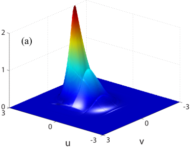
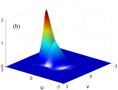
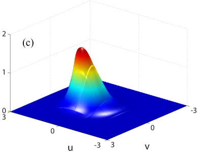
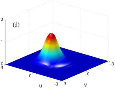
Figure 1: Relaxation of two Maxwellian streams using piece-wise quadratic DG approximations. Sections of the solution by plane $w=0$ are shown. The solutions correspond to $s_{u}=s_{v}=s_{w}=3$ and 7 cells in each velocity direction. (a) $t=0$ $\mu$s, (b) $t=1.3$ $\mu$s, (c) $t=7.6$ $\mu$s, and (d) $t=39.2$ $\mu$s.

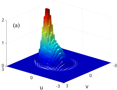
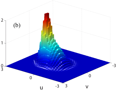
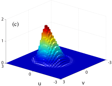
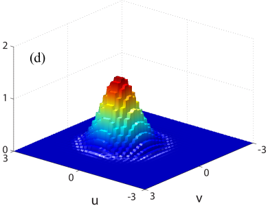
Figure 2: Relaxation of two Maxwellian streams using piece-wise constant DG approximations. Sections of the solution by plane $w=0$ are shown. The solutions correspond to $s_{u}=s_{v}=s_{w}=1$ and 33 cells in each velocity direction: (a) $t=0$ $\mu$s; (b) $t=1.3$ $\mu$s; (c) $t=7.6$ $\mu$s; and (d) $t=39.2$ $\mu$s.

In Figures 1 and 2 solutions to the relaxation of the two Maxwellian streams are shown. Simulations corresponding to $s_{u}=s_{v}=s_{w}=3$, $M=7$ are shown in Figure 1 and the simulation for $s_{u}=s_{v}=s_{w}=1$, $M=33$ in Figure 2. One-dimensional sections of the solution by planes $v=0$ and $w=0$ are shown in Figure 3. In Figure 3(a) the DG approximations of the initial data are given and in Figure 3(b) the approximations of the steady state are given. Both the piece-wise constant and the piece-wise quadratic case appear to capture the relaxation process successfully.

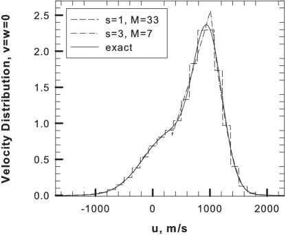
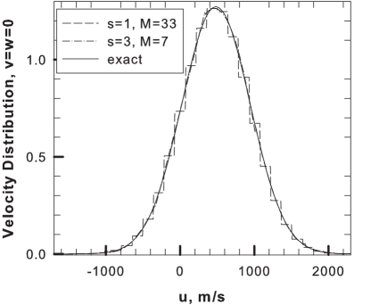
(a)	(b)

Figure 3: Cross sections of the solution to the problem of relaxation of two Maxwellian streams by planes $v=0$ and $w=0$. DG approximations with $s_{u}=s_{v}=s_{w}=1$, $M=27$ and $s_{u}=s_{v}=s_{w}=3$, $M=7$ are compared. (a) Approximations of the initial data. (b) Approximations of the steady state.

DG solutions were compared with the solutions obtained by established DSMC solvers [29]. In Figure 4(a) the ratios of directional temperatures $T_{x}$ and $T_{y}$ to the average temperature $T_{\mathrm{avg}}=T/3$ are shown. The solution reaches equilibrium state at about 45 $\mu$s. The DG approximation shows an excellent agreement with the DSMC solution. In Figure 4(b) relative errors in the solution temperature are presented for $s_{u}=s_{v}=s_{w}=3$, $M=5,7$ and $s_{u}=s_{v}=s_{w}=1$, $M=15,27$. In our DG approach no special enforcement of conservation laws is used. Rather, it is expected that similar to [24, 23] a satisfactory conservation can be achieved by using sufficiently refined DG approximations. It can be observed that for $s_{u}=s_{v}=s_{w}=33$, $M=7$ the temperature is computed correctly within three digits of accuracy. It was observed also that piece-wise constant approximations perform significantly better in this problem. This finding is consistent with [23] where it was found that piece-wise constant DG approximations are converging faster than high order DG approximations on smooth solutions. It is however expected that high order methods will be superior on the solutions that are not numerically smooth, e.g., due to truncation errors in spatially inhomogeneous problems.

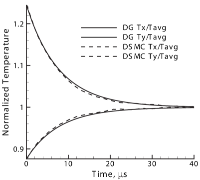
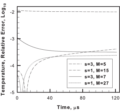
(a)	(b)

Figure 4: Relaxation of two Maxwellian streams. (a) Comparison of the DG solution to the DSMC solution by I. Boyd [29]. Ratios $T_{x}/T_{\mathrm{avg}}$ and $T_{y}/T_{\mathrm{avg}}$ are plotted. Here $T_{x}$ and $T_{y}$ are directional temperatures and $T_{\mathrm{avg}}=T/3$, where $T$ is the temperature of the exact solution. (b) Relative errors in the solutions temperature. Piece-wise quadratic and piece-wise constant DG approximations are compared. The piece-wise constant approximations are more accurate in this problem.

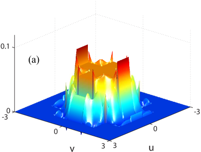
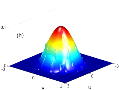
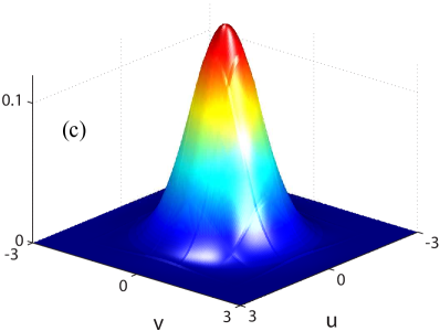
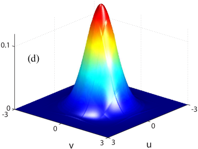
Figure 5: Relaxation of two artificial streams using piece-wise quadratic DG approximations. Sections of the solution by plane $w=0$ are shown. The solutions correspond to $s_{u}=s_{v}=s_{w}=3$ and 7 cells in each velocity direction. (a) $t=0$ ns, (b) $t=0.5$ ns, (c) $t=2.1$ ns, and (d) $t=4.5$ ns.

Our second problem is concerned with the relaxation of two artificial streams with discontinuous initial data. Specifically, the initial distribution is a sum of two functions of the form

$$f_{\mathrm{X}}(\vec{v})=\left\{\begin{array}[]{lr}\rho h,&\mbox{if}\ |\vec{v}-\vec{\bar{v}}|\leq r\,,\\ 0,&\mbox{if}\ |\vec{v}-\vec{\bar{v}}|>r\,,\end{array}\right.\ ,\quad r=(T/5R)^{1/2},\ \mbox{and}\ h=(15\sqrt{5}/4\pi)(R/T)^{3/2}.$$

Here $\rho$, $\vec{\bar{v}}$ and $T$ are given parameters. It is a straightforward exercise to verify that $\rho$, $\vec{\bar{v}}$ and $T$ coincide with the mass density, bulk velocity and temperature of the distribution $f_{\mathrm{X}}(\vec{v})$, correspondingly. The gas is argon. The values of the macroparameters for the two artificial streams are $\rho_{1}=0.332$ kg/m³, $\vec{\bar{v}}_{1}=(106.0,0,0)$ m/s, $T_{1}=300$ K and $\rho_{2}=0.332$ kg/m³, $\vec{\bar{v}}_{2}=(-106.0,0,0)$ m/s, $T_{2}=300$ K. Graphs of two-dimensional cross-sections of the initial distribution by plane $w=0$ are given in Figures 5(a) and 6(a). The mean time between molecular collisions is estimated to be about $0.39$ ns. The simulations are performed for $190$ ns. In Figure 5 the simulations are presented using piece-wise quadratic approximations, $s_{u}=s_{v}=s_{w}=3$, on $M=7$ cells in each velocity dimension and in Figure 6 using piece-wise constant approximations, $s_{u}=s_{v}=s_{w}=1$, on $M=27$ cells in each velocity dimension. One can see that the simulations are consistent in capturing the process of relaxation. The approximation artifacts visible in Figure 5(a) are caused by insufficient resolution. These artifacts subside as the distribution functions relaxes and gets smoother.

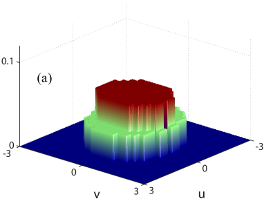
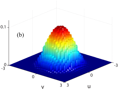
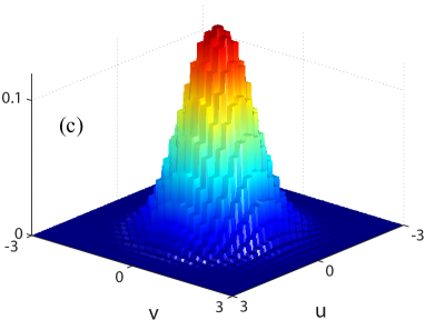
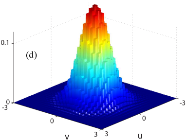
Figure 6: Relaxation of two artificial streams using piece-wise constant DG approximations. Sections of the solution by plane $w=0$ are shown. The solutions correspond to $s_{u}=s_{v}=s_{w}=1$ and 27 cells in each velocity direction. (a) $t=0$ ns; (b) $t=0.5$ ns; (c) $t=2.1$ ns; and (d) $t=4.5$ ns.

In Figure 7(b) the conservation of temperature in the DG solutions is given in the cases of $s_{u}=s_{v}=s_{w}=1$ and $s_{u}=s_{v}=s_{w}=3$. One can notice that the approximations of discontinuous initial data are less accurate and also that the piece-wise constant DG approximations perform inferior to the piece-wise quadratic approximations. This observation is consistent with studies performed in [23]. It is believed that the fast convergence of the piece-wise constant approximations in the problem of relaxation of two Maxwellian distributions was due to the solution smoothness and to the fact that kinetic solutions exponentially decrease at infinity. As can be seen from the second example, accuracy of integration in piece-wise constant approximations deteriorates dramatically if the approximated solution is not smooth. One can see that growth of numerical errors in piece-wise constant DG approximations is fastest at the initial stages of the relaxation, when the solution is still far from being smooth. As the solution is getting smoother, however, the accuracy of quadrature rules increases and the conservation laws are satisfied with a better accuracy. As a result, we observe almost no change in the errors once the solutions reaches the steady state.

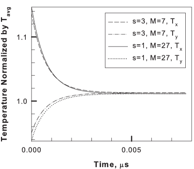
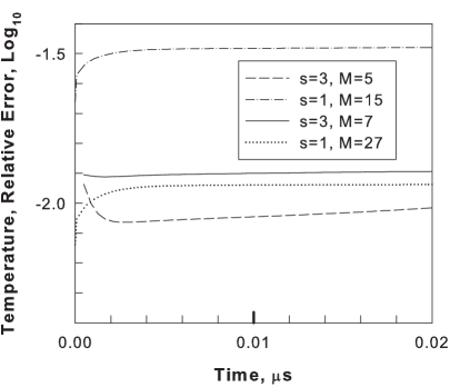
(a)	(b)

Figure 7: Relaxation of two artificial streams. (a) Ratios $T_{x}/T_{\mathrm{avg}}$ and $T_{y}/T_{\mathrm{avg}}$ are shown. Here $T_{x}$ and $T_{y}$ are directional temperatures and $T_{\mathrm{avg}}=T/3$. (b) Relative error in the solutions temperature. Piece-wise constant and piece-wise quadratic DG approximations are compared. Fast growth of error occurs in the piece-wise constant approximation at the initial stages of relaxation.

7 Conclusion

We developed a discontinuous Galerkin discretization of the Boltzmann equation in the velocity space using a symmetric bilinear form of the Galerkin projection of the collision operator. The time-independent kernel of the bilinear operator carries the information about the geometry of the velocity discretization and about the collision model. Properties of the kernel were studies and several practical statements about the kernel symmetry were formulated. Evaluation of the kernel was implemented using an MPI parallelization algorithm that scales to a large number of processors. The discontinuous Galerkin approach was applied to the problem of spatially homogeneous relaxation. Discretizations with up to $M=33$ degrees of freedom per velocity dimension were successfully tested on a single processor. DG solutions to the problem of spatially homogeneous relaxation showed excellent agreement with the solutions obtained by established DSMC codes. The solutions conserve mass momentum and temperature with a good accuracy.

The main obstacles to increasing the velocity resolution to hundreds of nodes per velocity dimension are the large amount of components per velocity basis function in the pre-computed collision kernel and the large number of resulting arithmetic operations to evaluate the collision integral. These numbers were demonstrated to grow as $O(n^{5})$ and $O(n^{8})$, respectively for a single spatial cell. To overcome this problem, the authors are developing algorithms for parallelization of the evaluation of the collision integral to up to thousands of processors. An additional improvement is expected by constructing efficient Galerkin basis so as to minimise the total number of degrees of freedom in velocity variable. The discrete Galerkin form of the Boltzmann equation offers unique insights to the numerical properties of its solution. In the future, the authors will explore the eigenstructure of the bilinear discrete collision kernel and connect the new knowledge to the familiar numerical properties of the solutions to the Boltzmann equation. It is anticipated that this study will lead to the construction of more efficient approximation techniques.

Appendix A Proofs of Theorems 4.1–4.3

Lemma 4.1.

Let operator $A(\vec{v},\vec{v}_{1};\phi^{j}_{i})$ be defined by (11) with all gas particles having the same mass and the potential of the particles interaction being spherically symmetric. Then $A(\vec{v},\vec{v}_{1};\phi^{j}_{i})$ is symmetric with respect to $\vec{v}$ and $\vec{v}_{1}$, that is

$$A(\vec{v},\vec{v}_{1};\phi^{j}_{i})=A(\vec{v}_{1},\vec{v};\phi^{j}_{i}),\qquad\forall\vec{v},\vec{v}_{1}\in\mathbb{R}^{3}.$$

Also,

$$A(\vec{v},\vec{v};\phi^{j}_{i})=0,\qquad\forall\vec{v}\in\mathbb{R}^{3}.$$

Proof.

Formula (13) follows immediately from (11) by noticing that if $\vec{v}=\vec{v}_{1}$ then $\vec{g}=0$. Therefore, (11) is automatically zero.

To prove (12) we recall that in the case when all particles have the same mass, the interchange of pre-collision velocities $\vec{v}$ and $\vec{v}_{1}$ will result in the interchange of post collision velocities $\vec{v}^{\prime}$ and $\vec{v}^{\prime}_{1}$. In particular, no different post-collision velocities result from the interchange of $\vec{v}$ and $\vec{v}_{1}$. The statement follows by noticing the symmetry of the expression under the integral (12) is both pairs of velocities.

For a more “mathematical” proof one may recall that in the case of a spherically symmetric potential the pre-collision velocities $\vec{v}$ and $\vec{v}_{1}$ and the post-collision velocities $\vec{v}^{\prime}$ and $\vec{v}^{\prime}$ of the molecules are located on a sphere with the center at $(\vec{v}+\vec{v}_{1})/2$ and the radius of $|\vec{g}|/2$, see for example [31]. Furthermore, from some geometrical and physical considerations on concludes that $\vec{v}$, $\vec{v}_{1}$, $\vec{v}^{\prime}$ and $\vec{v}^{\prime}$ form a plain rectangle. Then the statement follows by observing that the rectangle is determined by $\vec{v}$ and $\vec{v}_{1}$ in a unique way.) ∎

Lemma 4.2.

Let operator $A(\vec{v},\vec{v}_{1};\phi^{j}_{i})$ be defined by (11) and let the potential of molecular interaction be dependent only on the distance between the particles. Then $\forall\xi\in\mathbb{R}^{3}$

$$A(\vec{v}+\vec{\xi},\vec{v}_{1}+\vec{\xi};\phi^{j}_{i}(\vec{v}-\vec{\xi}))=A(\vec{v},\vec{v}_{1};\phi^{j}_{i})\,.$$

Proof.

Consider $A(\vec{v}+\vec{\xi},\vec{v}_{1}+\vec{\xi};\phi^{j}_{i}(\vec{v}-\vec{\xi}))$. We clarify that these notations mean that vectors $\vec{v}$ and $\vec{v}_{1}$ in (11) are replaced with $\vec{v}+\vec{\xi}$ and $\vec{v}_{1}+\vec{\xi}$ correspondingly and that basis function $\phi^{j}_{i}(\vec{v})$ is replaced with a “shifted” function $\phi^{j}_{i}(\vec{v}-\vec{\xi})$. We notice that the relative speed of the molecules with velocities $\vec{v}+\vec{\xi}$ and $\vec{v}_{1}+\vec{\xi}$ is still $\vec{g}=\vec{v}+\vec{\xi}-(\vec{v}_{1}+\vec{\xi}_{1})=\vec{v}-\vec{v}_{1}$. Since the potential of molecular interaction depends only on the distance between the particles and in particular it does not depend on the particles individual velocities, the post-collision velocities will be $\vec{v}^{\prime}+\vec{\xi}$ and $\vec{v}^{\prime}_{1}+\vec{\xi}$. The rest of the statement follows a direct substitution:

$$A(\vec{v} +\vec{\xi},\vec{v}_{1}+\vec{\xi};\phi^{j}_{i}(\vec{v}-\vec{\xi}))$$

$$=\frac{|\vec{g}|}{2}\int_{0}^{2\pi}\int_{0}^{b_{\ast}}(\phi^{j}_{i}((\vec{v}^{\prime}+\vec{\xi})-\vec{\xi})+\phi^{j}_{i}((\vec{v}^{\prime}_{1}+\vec{\xi})-\vec{\xi})-\phi^{j}_{i}((\vec{v}+\vec{\xi})-\vec{\xi})-\phi^{j}_{i}((\vec{v}_{1}+\vec{\xi})-\vec{\xi})b\,db\,d\varepsilon\,$$

$$=\frac{|\vec{g}|}{2}\int_{0}^{2\pi}\int_{0}^{b_{\ast}}(\phi^{j}_{i}(\vec{v}^{\prime})+\phi^{j}_{i}(\vec{v}^{\prime}_{1})-\phi^{j}_{i}(\vec{v})-\phi^{j}_{i}(\vec{v}_{1}))b\,db\,d\varepsilon\,$$

$$=A(\vec{v},\vec{v}_{1};\phi^{j}_{i})\,.$$

∎

Lemma 4.3.

Let operator $A(\vec{v},\vec{v}_{1};\phi^{j}_{i})$ be defined by (11) and let the potential of molecular interaction be dependent only on the distance between the particles. Let $S:\mathbb{R}^{3}\to\mathbb{R}^{3}$ be a linear isometry of $\mathbb{R}^{3}$. Then

$$A(S\vec{v},S\vec{v}_{1};\phi^{j}_{i}(S^{-1}\vec{u})=A(\vec{v},\vec{v}_{1};\phi^{j}_{i})\,.$$

Proof.

We begin with a remark that will be helpful to highlight the mathematical structure of the proof. In kinetic theory there is a connection between the velocity space and the physical space in that velocity vectors are describing motion in the physical space and that displacement vectors in physical space are naturally identified with points in the velocity space. By identifying this connection, we implicitly introduce an angle and orientation preserving affine transformation that maps the first axis of the positive coordinate triple in the physical space to the first axis of the positive coordinate triple in the velocity space, the second axis into the second one and the third axis into the third one. As a result, we obtain a way to map vectors from the physical space to the velocity space and vice-versa. Connection between physical and velocity spaces can also be seen in definition (11). Indeed, post-collision velocities $\vec{v}^{\prime}$ and $\vec{v}^{\prime}_{1}$ are functions of the pre-collision velocities, $\vec{v}$ and $\vec{v}_{1}$, the impact parameters $b$ and $\varepsilon$ and the collision model. While the former belongs to the velocity space, the latter belongs to the physical space. Moreover, to define parameters $b$ of the molecular shortest approach distance and $\varepsilon$ of the relative angle of the collision plane, we must move the vector of relative velocity $\vec{g}=\vec{v}-\vec{v}_{1}$ into the physical space, e.g., [30], Section 1.3. Specifically, we define $b$ as the distance from the center of the second molecule to the line coming through the center of the first molecule in the direction of their relative velocity $\vec{g}$. Also, the parameter $\varepsilon$ is the angle between the collision plane formed by the image of the vector $\vec{g}$ in the physical space and the centers of the colliding molecules and a reference coordinate plane. Thus, to evaluate (11) we need to map vectors between physical and velocity spaces many times. Applying this reasoning to the statement of the theorem in question, we notice that the left side of (15) is evaluated relative to velocities $S\vec{v}$ and $S\vec{v}_{1}$ while the right side relative to velocities $\vec{v}$ and $\vec{v}_{1}$. Therefore separate sets of impact parameters are introduced for each case. What we are intended to show is that the result is the same for both cases.

Applying definition (11) to the left side of (15) we have

$$A(S\vec{v}, S\vec{v}_{1};\phi^{j}_{i}(S^{-1}\vec{u}))$$

$$=\frac{|\vec{\tilde{g}}|}{2}\int_{0}^{2\pi}\int_{0}^{b_{\ast}}[\phi^{j}_{i}(S^{-1}(S\vec{v})^{\prime}))+\phi^{j}_{i}(S^{-1}(S\vec{v}_{1})^{\prime})-\phi^{j}_{i}(S^{-1}S\vec{v})-\phi^{j}_{i}(S^{-1}S\vec{v}_{1})]\tilde{b}\,d\tilde{b}\,d\tilde{\varepsilon}\,$$

$$=\frac{|\vec{g}|}{2}\int_{0}^{2\pi}\int_{0}^{b_{\ast}}[\phi^{j}_{i}(S^{-1}(S\vec{v})^{\prime})+\phi^{j}_{i}(S^{-1}(S\vec{v}_{1})^{\prime})-\phi^{j}_{i}(\vec{v})-\phi^{j}_{i}(\vec{v}_{1})]\tilde{b}\,d\tilde{b}\,d\tilde{\varepsilon}\,,$$ (18)

where $\vec{\tilde{g}}=S\vec{v}-S\vec{v}_{1}$ and $\tilde{b}$ and $\tilde{\varepsilon}$ are the impact parameters defined in the local coordinate system of the molecules with velocities $S\vec{v}$ and $S\vec{v}_{1}$. Notice that because $S$ is linear, we have $\vec{\tilde{g}}=S\vec{v}-S\vec{v}_{1}=S(\vec{v}-\vec{v}_{1})=S\vec{g}$. Also, $S$ is an isometry, therefore, $|\vec{\tilde{g}}|=|S\vec{g}|=|\vec{g}|$.

Let us now describe the local coordinate systems that are introduced for both pairs of molecules: the pair with velocities $S\vec{v}$ and $S\vec{v}_{1}$ and the pair with velocities $\vec{v}$ and $\vec{v}_{1}$. Let us consider the molecules with velocities $S\vec{v}$ and $S\vec{v}_{1}$, first. According to the formalism described above, we define $\tilde{b}$ as the distance from molecule with velocity $S\vec{v}_{1}$ to the line passing through the center of molecule with velocity $S\vec{v}$ in the direction of $\vec{\tilde{g}}$. We let the coordinate system be introduced for the pair of colliding molecules with velocities $S\vec{v}$ and $S\vec{v}_{1}$ so that its origin located at the center of the molecule with velocity $S\vec{v}$ and its $\tilde{\xi}_{1}$ axis directed along $\vec{\tilde{g}}$. Then the parameter $\tilde{b}$ is the distance to the $\tilde{\xi}_{1}$ axis. The parameter $\tilde{\varepsilon}$ of the angle of the collision plane is defined relevant to a reference plane. We let axes $\tilde{\xi}_{2}$ and $\tilde{\xi}_{3}$ be selected to make a right triple and designate the plane $\tilde{\xi}_{1}\tilde{\xi}_{2}$ as the reference plane. We note that the collision plane contains the $\tilde{\xi}_{1}$ axis and let the angle $\tilde{\varepsilon}$ between the reference plane and the collision plane be measured from $\tilde{\xi}_{2}$ axis toward the $\tilde{\xi}_{3}$ axis. Notice that these assumptions do not limit the generality of the argument because any admissible parametrization should produce the correct value of the integral above.

We will now show that a choice of the parameter $\varepsilon$ can be made in a local system of coordinates corresponding to the pair of molecules colliding with velocities $\vec{v}$ and $\vec{v}_{1}$, such that $\vec{v}^{\prime}=S^{-1}(S\vec{v})^{\prime}$ and $\vec{v}^{\prime}_{1}=S^{-1}(S\vec{v}_{1})^{\prime}$ as long as $b=\tilde{b}$ and $\varepsilon=\tilde{\varepsilon}$. We let the origin of the second set of coordinates be located at the center of molecule with velocity $\vec{v}$ and its ${\xi}_{1}$ axis directed along ${\vec{g}}$. Then parameter $b$ gives the distance from the molecule with velocity $\vec{v}_{1}$ to the axis $\xi_{1}$. We define axes ${\xi}_{2}$ and ${\xi}_{3}$ to be the images of $\tilde{\xi}_{2}$ and $\tilde{\xi}_{3}$, respectively, under the action of $S^{-1}$. Specifically, using the mapping between the physical space and the velocity space we consider the unit vectors giving the directions of the axes $\tilde{\xi}_{2}$ and $\tilde{\xi}_{3}$ in the velocity space. Let these vectors be $\vec{\tilde{\tau}}_{2}$ and $\vec{\tilde{\tau}}_{3}$, respectively. Applying the inverse transformation $S^{-1}$ to these vectors and moving back to physical space, we require that $\vec{\tau}_{2}=S^{-1}\vec{\tilde{\tau}}_{2}$ and $\vec{\tau}_{3}=S^{-1}\vec{\tilde{\tau}}_{3}$ be the unit vectors of the axes $\xi_{2}$ and $\xi_{3}$. It is a simple check that $\vec{\tau}_{1}=S^{-1}\vec{\tilde{\tau}}_{1}$, where $\vec{\tilde{\tau}}_{1}=\vec{\tilde{g}}/|\vec{\tilde{g}}|$ defines the $\tilde{\xi}_{1}$ axis.

Since the molecular potential is spherically symmetric, the relative velocity undergoes a specular reflection on the impact, see e.g. [31], Section 1.2. Furthermore, the trajectories of the colliding molecules are contained in the collision plane, see e.g., [30], Section 1.3. Thus the post-collision relative velocity belongs to the collision plane. Let us denote by $O[b,\varepsilon,|\vec{g}|](\vec{g}):\mathbb{R}^{3}\to\mathbb{R}^{3}$ the operator of flat rotation of the vector of relative velocity in collision plane. Notice that the rotation angle depends on the approach distance $b$, the collision model and on the norm of the relative velocity. It, however, does not depend on the direction of $\vec{g}$. Re-writing slightly the familiar formulas for the post-collision velocities (see, e.g., [31], Section 1.2), we have

$$\vec{v}^{\prime} =\vec{v}+(O[b,\varepsilon,|\vec{g}|](\vec{g})-\vec{g})/2\,,$$

$$\vec{v}^{\prime}_{1} =\vec{v}_{1}-(O[b,\varepsilon,|\vec{g}|](\vec{g})-\vec{g})/2\,.$$

Similarly the molecules with velocities $S\vec{v}$ and $S\vec{v}_{1}$ we have

$$(S\vec{v})^{\prime} =S\vec{v}+(O[\tilde{b},\tilde{\varepsilon},|\vec{\tilde{g}}|](\vec{\tilde{g}})-\vec{\tilde{g}})/2\,,$$

$$(S\vec{v}_{1})^{\prime} =S\vec{v}_{1}-(O[\tilde{b},\tilde{\varepsilon},|\vec{\tilde{g}}|](\vec{\tilde{g}})-\vec{\tilde{g}})/2\,.$$

recalling that $|\vec{\tilde{g}}|=|\vec{g}|$, we obtain

$$(S\vec{v})^{\prime} =S\vec{v}+(O[\tilde{b},\tilde{\varepsilon},|\vec{{g}}|](\vec{\tilde{g}})-\vec{\tilde{g}})/2\,,$$

$$(S\vec{v}_{1})^{\prime} =S\vec{v}_{1}-(O[\tilde{b},\tilde{\varepsilon},|\vec{{g}}|](\vec{\tilde{g}})-\vec{\tilde{g}})/2\,.$$ (19)

We now consider the two vectors $O[\tilde{b},\tilde{\varepsilon},|\vec{{g}}|](\vec{\tilde{g}})$ and $S(O[b,\varepsilon,|\vec{g}|](\vec{g}))$. Because $S$ is a linear isometry, it preserves angles between vectors. Therefore, for any $0<n<b^{\ast}$ the plane formed by the vectors $S(O[b,\varepsilon,|\vec{g}|](\vec{g}))$, $\vec{\tilde{g}}=S\vec{g}$ will be making angle $\varepsilon$ with the plane formed by vectors $\vec{\tilde{\tau}}_{2}=S\vec{{\tau}}_{2}$ and $\vec{\tilde{\tau}}_{3}=S\vec{{\tau}}_{3}$. Moreover, $S(O[b,\varepsilon,|\vec{g}|](\vec{g}))$ will make the same angle with vector $\vec{\tilde{g}}=S\vec{g}$ as $O[b,\varepsilon,|\vec{g}|](\vec{g})$ is making with $\vec{g}$. Recalling that the angle of flat rotation in (A) only depends on $\tilde{b}$ we conclude that if $\tilde{b}=b$ then $O[\tilde{b},\tilde{\varepsilon},|\vec{{g}}|](\vec{\tilde{g}})$ will make the same angle with $\vec{\tilde{g}}$ as $O[b,\varepsilon,|\vec{g}|](\vec{g})$ is making with $\vec{g}$. Noting that as long as $\tilde{\varepsilon}=\varepsilon$, both $S(O[b,\varepsilon,|\vec{g}|](\vec{g}))$ and $O[\tilde{b},\tilde{\varepsilon},|\vec{{g}}|](\vec{\tilde{g}})$ lay in the same plane, we conclude that they are the same vectors. Therefore, $S(O[b,\varepsilon,|\vec{g}|](\vec{g}))=O[\tilde{b},\tilde{\varepsilon},|\vec{{g}}|](\vec{\tilde{g}})$ and $O[b,\varepsilon,|\vec{g}|](\vec{g})=S^{-1}(O[\tilde{b},\tilde{\varepsilon},|\vec{{g}}|](\vec{\tilde{g}}))$ as long as $\tilde{b}=b$ and $\tilde{\varepsilon}=\varepsilon$. By applying $S^{-1}$ to both sides of (15) we conclude that $\vec{v}^{\prime}=S^{-1}(S\vec{v})^{\prime}$ and $\vec{v}^{\prime}_{1}=S^{-1}(S\vec{v}_{1})^{\prime}$ as long as $b=\tilde{b}$ and $\varepsilon=\tilde{\varepsilon}$. The rest of the statement follows by introducing the substitution $\tilde{b}=b$ and $\tilde{\varepsilon}=\varepsilon$ in (A) and replacing $S^{-1}(S\vec{v})^{\prime}$ and $S^{-1}(S\vec{v}_{1})^{\prime}$ with $\vec{v}^{\prime}$ and $\vec{v}^{\prime}_{1}$, respectively. ∎

We notice that in the case of a general molecular interaction potential, the angle of rotation in the collision plane included in $O[\tilde{b},\tilde{\varepsilon},|\vec{{g}}|]$, depends on the relative velocity. Because of this, it is unlikely that Lemma 4.3 can be extended to a contraction mapping $S$. We however anticipate that it is possible to develop analogs of formulas (15) by introducing an appropriate scaling parameter in the case of molecular potentials that do not depend on the relative velocity, e.g., for hard spheres. Such formulas would alleviate evaluation and storage of $A(\vec{v},\vec{v}_{1};\phi^{j}_{i})$.

References

- Bird [1994] G. Bird, Molecular Gas Dynamics and the Direct Simulation of Gas Flows, Clarendon Press, Oxford, 1994.
- Mohamad [2011] A. Mohamad, Lattice Boltzmann Method: Fundamentals and Engineering Applications with Computer Codes, 2011.
- Buet [1996] C. Buet, A discrete-velocity scheme for the Boltzmann operator of rarefied gas-dynamics, Transp. Theory Stat. Phys. 25 (1996) 33–60.
- Mieussens [2000] L. Mieussens, Discrete-velocity models and numerical schemes for the Boltzmann-BGK equation in plane and axisymmetric geometries, J. Comput. Physics 162 (2000) 429–466.
- Titarev [2012] V. A. Titarev, Efficient deterministic modelling of three-dimensional rarefied gas flows, Communications in Computational Physics 162 (2012) 162–192.
- Struchtrup [2005] H. Struchtrup, Macroscopic Transport Equations for Rarefied Gas Flows Approximation Methods in Kinetic Theory, Interaction of Mechanics and Mathematics Series, Springer, Heidelberg, 2005.
- Tcheremissine [2006] F. G. Tcheremissine, Solution to the boltzmann kinetic equation for high-speed flows, Computational Mathematics and Mathematical Physics 46 (2006) 315–329.
- Kolobov et al. [2007] V. Kolobov, R. Arslanbekov, V. Aristov, A. Frolova, S. Zabelok, Unified solver for rarefied and continuum flows with adaptive mesh and algorithm refinement, Journal of Computational Physics 223 (2007) 589 – 608.
- Aristov et al. [2004] V. Aristov, A. Frolova, S. Zabelok, Parallel algorithms of direct solving the boltzmann equation in aerodynamics problems, in: A. Ecer, N. Satofuka, J. Periaux, P. Fox (Eds.), Parallel Computational Fluid Dynamics 2003, Elsevier, Amsterdam, 2004, pp. 49 – 56.
- Josyula et al. [2011] E. Josyula, P. Vedula, W. F. Bailey, C. J. Suchyta, III, Kinetic solution of the structure of a shock wave in a nonreactive gas mixture, Physics of Fluids 23 (2011) 017101.
- Aristov and Zabelok [2002] V. V. Aristov, S. A. Zabelok, A deterministic method for the solution of the boltzmann equation with parallel computations, Zhurnal Vychislitel’noi Tekhniki i Matematicheskoi Physiki 42 (2002) 425–437.
- Bobylev and Rjasanow [1999] A. V. Bobylev, S. Rjasanow, Fast deterministic method of solving the Boltzmann equation for hard spheres, Eur. J. Mech. B/Fluids 18 (1999) 869–887.
- Aristov [2001] V. Aristov, Direct Methods for Solving the Boltzmann Equation and Study of Nonequilibrium Flows, Fluid Mechanics and Its Applications, Kluwer Academic Publishers, c, 2001.
- Pareschi and Russo [2000] L. Pareschi, G. Russo, Numerical solution of the boltzmann equation i: Spectrally accurate approximation of the collision operator, SIAM Journal on Numerical Analysis 37 (2000) pp. 1217–1245.
- Varghese [2007] P. L. Varghese, Arbitrary post-collision velocities in a discrete velocity scheme for the Boltzmann equation, in: M. Ivanov, A. Rebrov (Eds.), 25th International Symposium on Rarefied Gas Dynamics, 21–28 July 2006, Saint-Petersburg, Russia, Publishing House of Siberian Branch of RAS, Novosibirsk, Russia, 2007, p. 8.
- Panferov and Heintz [2002] V. A. Panferov, A. G. Heintz, A new consistent discrete-velocity model for the boltzmann equation, Mathematical Methods in the Applied Sciences 25 (2002) 571–593.
- Malkov and Ivanov [2011] E. A. Malkov, M. S. Ivanov, The phase space PIC method for solving the Boltzmann equation. part I., in: 42nd AIAA Thermophysics Conference 27-30 June 2011, Honolulu, Hawaiit, number 3626 in AIP Conference Proceedings, American Institute of Physics, 2011, p. 12.
- Morris et al. [2011] A. Morris, P. Varghese, D. Goldstein, Monte carlo solution of the boltzmann equation via a discrete velocity model, Journal of Computational Physics 230 (2011) 1265 – 1280.
- Malkov et al. [2012] E. A. Malkov, M. S. Ivanov, S. O. Poleshkin, Discrete velocity scheme for solving the Boltzmann equation accelerated with the GP GPU, in: 28th International Symposium on Rarefied Gas Dynamics, 9–13 July 2012, Zaragoza, Spain, AIP Conference Proceedings, American Institute of Physics, 2012, p. 8.
- Ghiroldi et al. [2012] G. Ghiroldi, L. Gibelli, P. Dagna, A. Invernizzi, Linearized Boltzmann equation: A preliminary exploration of its range of applicability, in: 28th International Symposium on Rarefied Gas Dynamics, 9-13 July 2012, Zaragoza, Spain, AIP Conference Proceedings, American Institute of Physics, 2012, p. 8.
- Alekseenko and Josyula [2012] A. Alekseenko, E. Josyula, Deterministic solution of the Equation using a discontinuous Galerkin velocity discretization, in: 28th International Symposium on Rarefied Gas Dynamics, 9-13 July 2012, Zaragoza, Spain, AIP Conference Proceedings, American Institute of Physics, 2012, p. 8.
- Mouhot et al. [2012] C. Mouhot, L. Pareschi, T. Rey, Convolute decomposition and fast summation methods for discrete-velocity approximations of the Boltzmann equation, Math. Mod. Num. Anal. (to appear) (2012) 5174–5187.
- Alekseenko [2011] A. M. Alekseenko, Numerical properties of high order discrete velocity solutions to the BGK kinetic equation, Appl. Numer. Math. 61 (2011) 410–427.
- Alekseenko et al. [2012] A. Alekseenko, N. Gimelshein, S. Gimelshein, An application of discontinuous Galerkin space and velocity discretisations to the solution of a model kinetic equation, International Journal of Computational Fluid Dynamics to appear (2012).
- Hesthaven and Warburton [2007] J. Hesthaven, T. Warburton, Nodal Discontinuous Galerkin Methods: Algorithms, Analysis, and Applications, Texts in Applied Mathematics, Springer, 2007.
- Bobylev [1997] A. V. Bobylev, Moment inequalities for the Boltzmann equation and applications to spatially homogeneous problems, J. Stat. Phys. 88 (1997) 1183–1214.
- Pareschi and Perthame [1996] L. Pareschi, B. Perthame, A fourier spectral method for homogeneous boltzmann equations, Transport Theory and Statistical Physics 25 (1996) 369–382.
- Par [2003] Computational methods and fast algorithms for Boltzmann equation, in: N. Bellomo, R. Gatignol (Eds.), Lecture notes on the discretization of the Boltzmann equation, volume 63 of Series on Advances in Mathematics and Applied Sciences, World Scientific, Singapore, 2003, pp. 159–202.
- Boyd [1991] I. D. Boyd, Vectorization of a monte carlo simulation scheme for nonequilibrium gas dynamics, Journal of Computational Physics 96 (1991) 411 – 427.
- Kogan [1969] M. Kogan, Rarefied Gas Dynamics, Plenum Press, New York, USA, 1969.
- Cercignani [2000] C. Cercignani, Rarefied Gas Dynamics: From Basic Concepts to Actual Caclulations, Cambridge University Press, Cambridge, UK, 2000.
- Gobbert and Cale [2007] M. K. Gobbert, T. S. Cale, A Galerkin method for the simulation of the transient 2-D/2-D and 3-D/3-D linear Boltzmann equation, J. Sci. Comput., 30 (2007) 237–273.
- Fox and Vedula [2010] R. O. Fox, P. Vedula, Quadrature-based moment model for moderately dense polydisperse gas-particle flows, Industrial and Engineering Chemistry Research 49 (2010) 5174–5187.
- Green and Vedula [2011] B. I. Green, P. Vedula, Validation of a collisional lattice boltzmann method, in: 20th AIAA Computational Fluid Dynamics Conference, 27-30 June 2011, Honolulu Hawaii, number 3403 in AIP Conference Proceedings, American Institute of Physics, 2011, p. 14.
- Gupta and Torrilhon [2012] V. K. Gupta, M. Torrilhon, Automated Boltzmann collision integrals for moment equations, in: 28th International Symposium on Rarefied Gas Dynamics, 9-13 July 2012, Zaragoza, Spain, AIP Conference Proceedings, American Institute of Physics, 2012, p. 8.
- Frigo et al. [1999] M. Frigo, C. Leiserson, H. Prokop, S. Ramachandran, Cache oblivious algorithms, in: 40th IEE Annual Symposium on Foundations of Computer Science, New York, October 1999, pp. 285–297.