Entropic Inference: some pitfalls
and paradoxes we can avoid

Abstract

The method of maximum entropy has been very successful but there are cases where it has either failed or led to paradoxes that have cast doubt on its general legitimacy. My more optimistic assessment is that such failures and paradoxes provide us with valuable learning opportunities to sharpen our skills in the proper way to deploy entropic methods.

The central theme of this paper revolves around the different ways in which constraints are used to capture the information that is relevant to a problem. This leads us to focus on four epistemically different types of constraints. I propose that the failure to recognize the distinctions between them is a prime source of errors.

I explicitly discuss two examples. One concerns the dangers involved in replacing expected values with sample averages. The other revolves around misunderstanding ignorance. I discuss the Friedman-Shimony paradox as it is manifested in the three-sided die problem and also in its original thermodynamic formulation.

1 Introduction

Our subject is entropic inference. The method of maximum entropy (whether in its original MaxEnt version or its generalization ME, the method for updating probabilities) has been successful in many applications but there are cases where it has either failed or led to paradoxes. It has been suggested that these are symptoms of irreparable flaws. I disagree. My assessment is considerably more optimistic: the paradoxes provide us with valuable opportunities for learning how to use the method and equally valuable warnings about pitfalls we can and should avoid.

First, some background. The objective of the method of maximum entropy (ME) is to update from a prior distribution $q$ to a posterior distribution when information is given that the posterior $P$ is constrained to belong to a certain family of distributions: $P\in\mathcal{C}=\{p\}$. The selected posterior $P$ is that which maximizes the (relative) entropy

$$S[p,q]=-\int dx\,p(x)\log\frac{p(x)}{q(x)}~{}$$ (1)

subject to the constraint $\mathcal{C}$. Justifying the method revolves to a large extent around justifying the particular choice of the functional $S[p,q]$. The criteria involved in designing the functional $S[p,q]$ are purely pragmatic:

(1) We seek a method of universal applicability. It is conceivable that different situations could require different induction methods but what we want is a general-purpose method that captures what all those other problem-specific methods have in common.

(2) We want a parsimonious method that recognizes the value of information. What has been laboriously learned in the past should not be disregarded unless rendered obsolete by new information. Priors matter: rational beliefs should be updated but only to the minimal extent demanded by the new information.

(3) The method must be useful in practice. In particular, in order to do science we must be able to understand parts of the universe without having to understand the universe as a whole. This implies that the notion of statistical independence must play a central and privileged role. This idea – that some things can be neglected, that not everything matters – is implemented by imposing a criterion that tells us how to handle independent systems. The design criterion we adopt is quite natural: Whenever two systems are a priori believed to be independent and we receive information about one it should not matter if the other is included in the analysis or not.

The subtleties of how these criteria are implemented by imposing locality, coordinate invariance, and independence and the proofs showing that they lead to the entropy functional (1) are discussed in [8]. A noteworthy feature is that it is not necessary to provide an interpretation for $S[p,q]$ be it in terms of heat, or disorder, or amounts of information. Entropy is a tool for updating that requires no further interpretation.

The task of entropic inference – to update rational beliefs when information becomes available – immediately points both to the question “What is information?” and to its answer. A fully Bayesian information theory demands a close relation between information and the beliefs of an ideally rational agent and, accordingly, the answer is: information is that which affects rational beliefs, and thus, constraints are information. Which leads us to the main topic of this paper: how to deploy constraints that correctly capture the information that is relevant to a problem. In the next section I argue that we ought to distinguish four epistemically different cases and that the failure to recognize the distinctions among them is a prime source of mistakes and paradoxes.

Over the years a number of objections have been raised against the method of maximum entropy. I believe some of these objections were quite legitimate at the time they were raised. They uncovered conceptual pitfalls with the old MaxEnt as it was understood at the time. I also believe that in the intervening decades our understanding of entropic inference has evolved to the point that all these concerns can now be addressed satisfactorily. I explicitly discuss two examples of such mistakes. One concerns the dangers of replacing expected values with sample averages (a good discussion of this so-called “constraint rule” is e.g. [9]). The other revolves around misunderstanding ignorance. These are objections of the type raised by the Friedman-Shimony paradox [10][11] as it is manifested in the three-sided die problem [9][12] and also in its original thermodynamic formulation.

2 On constraints and relevant information

To fix ideas consider the standard MaxEnt problem: to assign the probability of a discrete variable $i$ assuming a uniform underlying measure $q_{i}=$ const and information in the form of a single linear constraint, $\langle f\rangle=F$. MaxEnt requires us to maximize the Shannon entropy $S[p]=-\textstyle\sum_{i}p_{i}\log p_{i}$ subject to $\langle f\rangle=F$ and $\textstyle\sum_{i}p_{i}=1$ which yields $p(i|\lambda)\propto e^{-\lambda f_{i}}$ for an appropriately chosen $\lambda$.

For example, the canonical distribution that describes the state of thermodynamic equilibrium is obtained maximizing $S[p]$ subject to a constraint on the expected energy $\langle\varepsilon\rangle=E$. This yields the Boltzmann distribution, $p(i|\beta)\propto e^{-\beta\varepsilon_{i}}$, where $\beta=1/T$ is the inverse temperature. The questions that concern us here are: How do we decide which is the right constraint function $f$ to choose? How do we decide the numerical value $F$ of its expectation? When can we expect the inferences to be reliable?

When using the MaxEnt method to obtain, say, the Boltzmann distribution it has been common to adopt the following language:

  

We seek the probability distribution that codifies the information we actually have (e.g., the expected energy) and is maximally unbiased (i.e. maximally ignorant or maximum entropy) about all the other information we do not possess.

This justification has stirred considerable controversy. Some of the objections that have been raised are the following:

O1

Objective reality is independent of our subjective knowledge about it. The observed spectrum of black body radiation is what it is independently of whatever information happens to be available to us.

O2

In most realistic situations the expected value of the energy is not a quantity we happen to know. How, then, can we justify using it as information we actually have?

O3

Even when the expected values of some quantities happen to be known, there is no guarantee that the resulting inferences will be any good at all. How can we justify the success of thermodynamics?

These objections deserve our consideration.

The issue raised by O1 concerns the very essence of what physical theories are meant to be. Let us grant for the sake of argument that there is such a thing as an external reality, that real phenomena are what they are independently of our thoughts about them. Then the issue raised by O1 is whether the purpose of our theories is to provide models that faithfully mirror this external reality or whether the connection to reality is considerably more indirect and the models are pragmatic tools for manipulating information about reality for the purposes of prediction, control, explanation, etc. In the former case theories mirror reality and there is no logical room for subjectivity. In the latter case theories deal with our information about reality and some subjective elements are inevitable. The evidence in favor of the latter alternative is already considerable. It includes the successful derivation and a host of insights into statistical mechanics and thermodynamics achieved by Jaynes’ MaxEnt. It also includes the more recent entropic/Bayesian derivations of both quantum and classical mechanics.

The objection O1 originates in a failure to recognize that while those epistemic judgments that must be made when assigning probabilities are inevitably subjective, they can nevertheless still be objectively right or wrong depending on whether they achieve empirical success or not. Thus, we can evade O1 by refusing to wear a straightjacket that forces us into a strict subjective/objective dichotomy. Subjective judgments do not preclude inferences that are objectively correct or incorrect.

To address objections O2 and O3 it is useful to distinguish four epistemically different types of constraints:

(A)

We know that the expected value of the function $f$ captures information that happens to be relevant to the particular problem at hand and we also know its numerical value, $\langle f\rangle=F$.

The ideal situation is one in which the set of available constraints of type A is complete in the sense that all the information that is necessary to obtain reliable answers to the questions that interest us is available. Only then are we guaranteed reliable predictions. Both requirements of relevance and completeness are crucial: an incomplete set of type A constraints has predictive value in that it leads to the best predictions that one can achieve under the circumstances but there is no guarantee that the predictions will be any good. Thus we see that, properly understood, objection O3 is not a flaw of the entropic method; it is a legitimate warning that reasoning with incomplete information is a risky business.

Note that a particular piece of evidence can be relevant and complete for some questions but not for others. For example, the expected energy $\langle\varepsilon\rangle=E$ is both relevant and complete for the question “Will system 1 be in thermal equilibrium with another system 2?” or alternatively, “What is the temperature of system 1?” But the same expected energy is far from complete for the vast majority of other possible questions such as, for example, “Where can we expect to find molecule #23 in this sample of ideal gas?”

(B)

We know that $\langle f\rangle$ captures information that happens to be relevant to the problem at hand but its actual numerical value $F$ is not known.

This is the most common situation in physics. The answer to objection O2 hinges on the observation that whether the value of the expected energy $E$ is known or not, it is nevertheless still true that maximizing entropy subject to the energy constraint $\langle\varepsilon\rangle=E$ leads to the objectively correct family of distributions that describe thermal equilibrium (including, for example, the observed black-body spectral distribution). Thus, the justification behind imposing a constraint on the expected energy is not that the quantity $E$ happens to be known – because of the brute fact that its value is never actually known – but rather that it is a quantity that should be known. Even when the actual numerical value $E$ is unknown, the epistemic situation described in case B is one in which we know that the expected energy $\langle\varepsilon\rangle$ is the relevant information without which no successful predictions are possible.

The question of how a particular $f$ is singled out as relevant has to be tackled on a case by case basis. In [8] we discuss the problem of thermal equilibrium and show that the relevant quantity is indeed the expected energy $\langle\varepsilon\rangle$ and not some other conserved quantity such as $\langle\varepsilon^{2}\rangle$ or $\langle f(\varepsilon)\rangle$.

Type B information is processed by allowing MaxEnt to proceed with the numerical value of $\langle\varepsilon\rangle=E$ handled as a free parameter. This leads us to the correct family of distributions $p(i|\beta)\propto e^{-\beta\varepsilon_{i}}$ containing the multiplier $\beta$ as a free parameter. The actual value of the parameter $\beta$ is at this point unknown and the standard approach is to seek additional information and infer $\beta$ either by a direct measurement using a thermometer, or to infer it indirectly by Bayesian parameter estimation from other empirical data. The additional information has the net effect of transforming the type B constraint into a type A.

(C)

There is nothing special about the function $f$ except that we happen to know its expected value, $\langle f\rangle=F$. In particular, we do not know whether information about $\langle f\rangle$ is complete or whether it is at all relevant to the problem at hand.

We do know something and this information, although limited, has some predictive value because it serves to constrain our attention to the subset of probability distributions that agree with it. Maximizing entropy subject to such a constraint will yield predictions that are the best possible under the circumstances but since we do not know that $f$ captures information that is relevant and complete there is absolutely no guarantee that the predictions will be any good. Induction is risky and objection O3 is a healthy reminder.

(D)

We know neither that $\langle f\rangle$ captures relevant information nor do we know its numerical value $F$.

This is an epistemic situation that reflects complete ignorance. Case D applies to any arbitrary function $f$ and therefore it applies equally to all functions. Since no specific $f$ is singled out a type D constraint provides no information at all and the correct procedure is to maximize $S[p]$ subject to the single constraint of normalization. The result is as it should be: extreme ignorance is described by a uniform distribution.

What distinguishes type C from D is that in C the value of $F$ is actually known. This fact singles out a specific variable $f$ and justifies using $\langle f\rangle=F$ as a constraint. What distinguishes D from B is that in B there is actual knowledge that singles out the variable $f$ as being relevant.

Objection O2 arises from a failure to distinguish constraints of type B from those of type C and D.

Summary: Between one extreme of ignorance (type D, we know neither which variables are relevant nor their expected values), and the other extreme of useful knowledge (a complete set of type A constraints in which we know all the relevant variables that need to be included in the analysis and we also know their expected values), there are intermediate states of knowledge (involving constraints of types B and C) and these constitute the rule rather than the exception. (It is, of course, also possible to encounter situations that mix constraints of different types.) Type B is the more common and important situation in which a relevant variable has been correctly identified even though its actual expected value might be unknown. The situation described as type C is less common because information about expected values is not usually available. (What might be easily available is information in the form of sample averages which is not in general quite the same thing — see the next section.) Type D constraints carry no information at all and should be ignored.

The considerations above also apply to the problem of entropic updating from a generic prior $q$ to a posterior by maximizing $S[p,q]$ subject to information in the form of constraints.

3 Sample averages are not expected values

Let us return to the question “If constraints refer to the expectation of certain variables, how do we decide their numerical magnitudes?” and explore some pitfalls. Here is a common temptation: the numerical values of expectations are seldom known and it is tempting to follow the “constraint rule” and replace expected values by sample averages because it is the latter that are directly available from experiment. But the two are not the same: Sample averages are experimental data. Expected values are not experimental data.

For very large samples such a replacement can be justified by the law of large numbers — there is a high probability that sample averages will approximate the expected values. However, for small samples using one as an approximation for the other can lead to incorrect inferences. It is important to realize that these incorrect inferences do not represent an intrinsic flaw of the entropic method; they are merely an indication of how the method should not to be used.

Example — just data:

Here is a variation on the same theme. Suppose data $D=(x_{1},x_{2}\ldots x_{n})$ have been collected. How do we process such information? Suppose we do not have a likelihood function so Bayes rule is not an option. We might be tempted to maximize $S[p,q]$ subject to a constraint $\langle x\rangle=C_{1}$ where $C_{1}$ is unknown and then try to estimate $C_{1}$ as a sample average. This is a dangerous move. The reason is that in the absence of additional information we know neither that $x$ constitutes relevant information nor do we know its expected value $C_{1}$ and therefore this is what we identified above as a type D constraint — no information at all.

The mistake becomes apparent when we realize that if we know the data $(x_{1},\ldots)$ then we also know their squares $(x_{1}^{2},\ldots)$ and their cubes and also any arbitrary function of them $(f(x_{1}),\ldots)$. And we also know the corresponding sample averages. Which of these should we use as an expected value constraint? Or should we use all of them? The answer is that the entropic method is not designed to tackle problems where the only information is data $D=(x_{1},x_{2}\ldots x_{n})$. It is not that it gives a wrong answer; it gives no answer at all because there is no constraint to impose; the entropic engine cannot even get started.

But there is a possible exception: surely the data $(x_{1},\ldots)$ must be relevant to inferences about the quantity $x$ itself. More generally, whether a given piece of data turns out to be relevant or not depends on what is the question being asked. If we want to make inferences about a particular function $f(x)$ then we know that information about $\langle f(x)\rangle$ must surely be relevant — in which case we deal with a type B constraint. Whether the information captured by $\langle f(x)\rangle$ is sufficient for reliable inferences, or whether higher moment constraints, $\langle f^{2}\rangle,\langle f^{3}\rangle\ldots$ must also be included is a question that must be addressed on a case by case basis.

Example — a type B constraint plus data:

Suppose then, that in addition to the data $D=(x_{1},x_{2}\ldots x_{n})$ collected in $n$ independent experiments we have information described as type B in the previous section: the expectation $\langle f\rangle$ captures relevant information. Then we can proceed to maximize the entropy $S[p,q]$, where $q(x_{i})$ is a (possibly uniform) prior distribution, subject to the constraint $\langle f\rangle=F$ where the unknown $F$ is treated as a free parameter. If the variable $x$ can take $k$ discrete values labeled by $i$ we let $q(x_{i})=q_{i}$ and $f(x_{i})=f_{i}$ and the result is a canonical distribution

$$p(x_{i}|\lambda)=\frac{1}{Z}q_{i}e^{-\lambda f_{i}}~{},$$ (2)

where

$$Z=\sum\limits_{i=1}^{k}q_{i}\,e^{-\lambda f_{i}}\quad\text{and}\quad\langle f\rangle=-\frac{\partial\log Z}{\partial\lambda}$$ (3)

with an unknown multiplier $\lambda$ that can be estimated from the data $D$ using standard Bayesian methods. Assuming the $n$ experiments are independent then Bayes rule gives,

$$p(\lambda|D)=\frac{p(\lambda)}{p(D)}\prod\limits_{j=1}^{n}\frac{1}{Z}q_{j}e^{-\lambda f_{j}}~{},$$ (4)

where $p(\lambda)$ is the prior for $\lambda$. It is convenient to consider the logarithm of the posterior,

$$\log p(\lambda|D)=\log p(\lambda)-\log p(D)-\sum\limits_{j=1}^{n}(\log Z-\log q_{j}+\lambda f_{j})~{}.$$

The value of $\lambda$ that maximizes the posterior $p(\lambda|D)$ is such that

$$0=\frac{\partial\log p(\lambda)}{\partial\lambda}-n\frac{\partial\log Z}{\partial\lambda}-n\bar{f}~{}.$$ (5)

where $\bar{f}$ is the sample average,

$$\bar{f}=\frac{1}{n}\sum\limits_{j=1}^{n}f_{j}~{}.$$ (6)

Using (3) we see that the expected value $\langle f\rangle$ (and its corresponding $\lambda$) can be estimated from the data as

$$\langle f\rangle=\bar{f}-\frac{1}{n}\frac{\partial\log p(\lambda)}{\partial\lambda}~{}.$$ (7)

As $n\rightarrow\infty$ the second term on the right hand side vanishes and we see that the optimal $\lambda$ is such that $\langle f\rangle=\bar{f}$. This is to be expected: as is usual in Bayesian inference for large $n$ the data $D$ overwhelms the prior $p(\lambda)$ and $\bar{f}$ tends to $\langle f\rangle$ (in probability). But the result eq.(7) also shows that when $n$ is not large then the prior can make a non-negligible contribution. In general one should not assume that $\langle f\rangle\approx\bar{f}$ .

Let us emphasize that this analysis holds only when there is additional knowledge to the effect that the specific variable $f$ captures relevant information. In the absence of such knowledge we are back to the previous example – just data – and we have no reason to prefer the function $f(x)$ over any other function $g(x)$ and accordingly we have no reason to prefer the distribution (2) over any other canonical distribution $q_{i}e^{-\lambda g_{i}}/Z$.

4 Confusion about ignorance

To set the stage for the issues involved consider a three-sided die. Its faces are labeled by the number of spots $i=1,2,3$ and have probabilities $\theta_{1},\theta_{2},\theta_{3}$ which will be collectively denoted by $\theta$. The space of distributions is the simplex $\mathcal{S}_{2}$ with $\textstyle\sum\nolimits_{i}\theta_{i}=1$ as shown in the figure. A fair die is one for which $\theta=\theta_{C}=(\frac{1}{3},\frac{1}{3},\frac{1}{3})$ which lies at the very center of the simplex. The expected number of spots for a fair die is $\langle i\rangle=2$. Having $\langle i\rangle=2$ is no guarantee that the die is fair but if $\langle i\rangle\neq 2$ the die is necessarily biased.

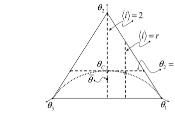
Figure 1: Constraints $\langle i\rangle=r$ are shown as vertical lines on the simplex. The dotted line is the set of MaxEnt distributions $\theta_{ME}(r)$ as $r$ spans the range from $1$ to $3$. If $r$ is unknown the average of $\theta_{ME}(r)$ over $r$ leads to the distribution marked by $\bar{\theta}$.

The paradox discussed by Friedman and Shimony [10] and further explored in [11], [12] and [9] arises from analyzing a situation of complete ignorance in two ways that are (mistakenly) thought to be equivalent.

Here is the first way to express complete ignorance:

Ignorance₁ — Nothing is known about the die; we do not know that it is fair but on the other hand there is nothing that induces us to favor one face over another. On the basis of this minimal information we can use MaxEnt. Maximize

$$S(\theta)=-\sum\nolimits_{i}\theta_{i}\log\theta_{i}$$ (8)

subject to $\sum\nolimits_{i}\theta_{i}=1$ and the resulting maximum entropy distribution is $\theta_{ME}=\theta_{C}$.

To set the background for the second way to represent complete ignorance consider constraints of the form $\langle i\rangle=r$ with $1\leq r\leq 3$. In the figure the constraints corresponding to $r=2$ and to a generic $r$ are shown as vertical dashed lines. Maximizing $S(\theta)$ subject to $\langle i\rangle=2$ and normalization leads us to assign $\theta_{ME}=\theta_{C}$ at the center of the simplex. Maximizing $S(\theta)$ subject to $\langle i\rangle=r$ and normalization leads to the point where the $r$ line crosses the dotted line. The dotted curve is the set of MaxEnt distributions $\theta_{ME}(r)$ as $r$ spans the range from $1$ to $3$.

Here is the second way to express complete ignorance:

Ignorance₂ — It is tempting (but wrong!) to pursue the following line of thought. We have a die but we do not know much about it. We do know, however, that the quantity $\langle i\rangle$ must have some value, call it $r$, about which we are ignorant too. Now, the most ignorant distribution given $r$ is the MaxEnt distribution $\theta_{ME}(r)$. But $r$ is itself unknown so a more honest assignment for $\theta$ would be an average over $r$,

$$\bar{\theta}=\int dr\,p(r)\theta_{ME}(r)~{},$$ (9)

where $p(r)$ reflects our uncertainty about $r$. It may, for example, make sense to pick a uniform distribution over $r$ but the precise choice is not important for our purposes. The point is that since the MaxEnt dotted curve is concave the point $\bar{\theta}$ necessarily lies below $\theta_{C}$ so that $\bar{\theta}_{2}<1/3$. And we have a paradox: we started assuming complete ignorance and through a process that claims to express full ignorance at every step we reach the conclusion that the die is biased against $i=2$. Where is the mistake?

Another way to expose the problem is to force the issue and impose that the two descriptions of complete ignorance be equivalent by fiat,

$$\theta_{C}=\bar{\theta}~{}.$$ (wrong)

Since the dotted line is concave this equality can only be achieved if $p(r)=\delta(r-2)$. And, again, we have a paradox: we started admitting complete ignorance about the die and therefore also about the value of $r$ and we end with complete certainty that $r=2$. Where is the mistake?

Before we blame the entropic method of inference it is best to take a closer look at Ignorance₂. One clue is symmetry. A situation of complete ignorance ought to treat the outcomes $i=1,2,3$ symmetrically but the end result is a distribution that is biased against $i=2$. The symmetry must have been broken somewhere and it is clear that this happened at the moment we imposed the constraint on $\langle i\rangle=r$ which is shown as vertical lines on the simplex. Had we chosen to express our ignorance not in terms of the unknown value of $\langle i\rangle=r$ but in terms of some other function $\langle f(i)\rangle=s$ then we could have easily broken the symmetry in some other direction. For example, let $f(i)$ be a cyclic permutation of $i$,

$$f(1)=2,\quad f(2)=3,\quad\text{and}\quad f(3)=1~{},$$ (10)

then repeating the analysis above would lead us to conclude that $\bar{\theta}_{1}<1/3$, which represents a die biased against $i=1$. Thus, the question becomes: What leads us to choose a constraint on $\langle i\rangle$ rather than a constraint on $\langle f(i)\rangle$ when we are equally ignorant about both?

The discussion in section 2 is relevant here. The paradox with the three-sided die arises because a constraint of type D has been treated as if it were a constraint of type B. The correct approach is to recognize that we do not know whether it is the constraint $\langle i\rangle$ or any other function $\langle f\rangle$ that captures relevant information and their numerical values $r$ are also unknown — clearly a type D constraint. There is nothing to single out $\langle i\rangle$ or any other $\langle f\rangle$ and therefore the correct inference consists of maximizing $S$ imposing the only constraint we actually know, namely, normalization. The result is as it should be — a uniform distribution ($\theta_{ME}=\theta_{C}$) which agrees with Ignorance₁.

On the other hand, the Ignorance₂ argument that led to the assignment of $\bar{\theta}$ in eq.(9) and to $\bar{\theta}_{2}<1/3$ would have been correct if we actually had knowledge that it is the particular variable $\langle i\rangle$ – and not any other $\langle f\rangle$ – that captures information that is relevant to this very particular die. Thus, imposing the type B constraint $\langle i\rangle=r$ when $r$ is unknown and then averaging over $r$ represents a situation in which we know something. There is some ignorance here – we do not know $r$ – but this is not extreme ignorance.

We can summarize as follows: knowing that the die is biased against $i=2$ but not knowing by how much (Ignorance₂) is not the same as not knowing anything about the die (Ignorance₁).

A thermodynamic version of the paradox is discussed in [11]. Here is the background: A physical system can be in any of $n$ microstates labeled $i=1\ldots n$. When we know absolutely nothing about the system (Ignorance₁) maximizing entropy subject to the single constraint of normalization leads to a uniform probability distribution,

$$p_{U}(i)=1/n~{}.$$ (11)

A different (and wrong!) way to express complete ignorance (Ignorance₂) is to argue that the expected energy $\langle\varepsilon\rangle$ must have some value $E$ about which we are ignorant. Maximizing entropy subject to both $\langle\varepsilon\rangle=E$ and normalization leads to the usual Boltzmann distributions,

$$p(i|\beta)=\frac{e^{-\beta\varepsilon_{i}}}{Z(\beta)}\quad\text{where}\quad Z(\beta)=\sum\limits_{i}e^{-\beta\varepsilon_{i}}~{}.$$ (12)

Since the inverse temperature $\beta=\beta(E)$ is itself unknown we must average over $\beta$,

$$\bar{p}(i)=\int d\beta\,p(\beta)p(i|\beta)~{}.$$ (13)

To the extent that both distributions are thought to reflect complete ignorance we must impose

$$p_{U}(i)=\bar{p}(i)$$ (wrong again)

which can be shown (see [11]) to imply that

$$p(\beta)=\delta(\beta)\quad\text{or}\quad\beta=0~{}.$$ (14)

Indeed, setting the Lagrange multiplier $\beta=0$ in $p(i|\beta)$ leads to the uniform distribution $p_{U}(i)$. And now we have a paradox: complete ignorance about the system (Ignorance₁) implies we are ignorant about its temperature. In fact, the system might not be in thermal equilibrium in which case it may not even have a temperature at all. But we also have the second way of expressing ignorance (Ignorance₂) and if we impose that the two agree we are led to conclude that $\beta$ has the value $\beta=0$ so that the temperature is precisely known. From complete ignorance we have (wrongly) concluded that the system must be infinitely hot — confusion about ignorance is hell.

The paradox is dissolved once we realize that, just as with the die problem, a type D constraint has been treated as type B. Knowing nothing about a system means we do not know whether it is in equilibrium or not. We do not know whether it is isolated and whether its energy is conserved and therefore it is not clear that $\langle\varepsilon\rangle$ might even be relevant information. This is the kind of non-information we earlier called a type D constraint that ought to be ignored.

On the other hand if we were to have actual knowledge that the system is in thermal equilibrium then it would be legitimate to impose a constraint on the expected energy $\langle\varepsilon\rangle$ — as discussed in [8] thermal equilibrium is the physical condition that singles out the expected energy $\langle\varepsilon\rangle$ as being the relevant piece of information. Since the temperature is unknown this is a type B constraint.

To summarize: knowing that a system is in thermal equilibrium while being ignorant about its temperature is not the same as knowing nothing about the system.

It may be worthwhile to rephrase this important point in yet another way. Let $i\in\mathcal{I}$ and $\beta\in\mathcal{B}$ where $\mathcal{I}$ is the space of microstates and $\mathcal{B}$ is the space of some arbitrary quantities $\beta$. The rules of probability theory allow us to write

$$p(i)=\int d\beta\,p(i,\beta)\quad\text{where}\quad p(i,\beta)=\,p(\beta)p(i|\beta)~{}.$$ (15)

Paradoxes will easily arise if we fail to distinguish a situation of complete ignorance from a situation where we have actual knowledge about the conditional probability $p(i|\beta)$, which is what gives the parameter $\beta$ its meaning as inverse temperature.

5 Summary

In entropic inference information is represented by constraints. In this tutorial we have argued that when constraints are expressed in terms of expected values the same formal expression $\langle f\rangle=F$ can be used to represent four different types of available information and failure to distinguish between them can lead to errors.

In decreasing order of useful information the types range from type A, in which we know that the quantity $f$ is relevant to the inference at hand and its expected value $F$ is known; to type B, in which $f$ is known to be relevant but $F$ is unknown; and type C, in which $f$ is of interest only because $F$ happens to be known. Constraints of type A and B are common and therefore important; type C constraints are less so because information about expected values (as opposed to sample averages) is less directly available.

Finally, there are situations of no information at all, labeled as type D, in which we know neither that $f$ is relevant nor its expected value $F$. The point of identifying and labeling the non-informative type D is precisely as to avoid the errors that arise from confusing D with the more informative types A, B, and C.

The usefulness of distinguishing these four types was illustrated by discussing the constraint rule and the Friedman-Shimony paradox.
Acknowledgements: I am grateful to Néstor Caticha, R. Fischer, A. Giffin, A. Golan, R. Preuss, C. Rodríguez, T. Seidenfeld, J. Skilling and J. Uffink for many useful discussions on entropic inference.

References

- [1] E. T. Jaynes, Probability Theory: The Logic of Science, ed. by L. Bretthorst (Cambridge U.P., 2003).
- [2] J. E. Shore and R. W. Johnson, IEEE Trans. Inf. Theory IT-26, 26 (1980); IEEE Trans. Inf. Theory IT-27, 26 (1981).
- [3] P. M. Williams, Brit. J. Phil. Sci. 31, 131 (1980).
- [4] J. Skilling, “The Axioms of Maximum Entropy” in Maximum-Entropy and Bayesian Methods in Science and Engineering, G. J. Erickson and C. R. Smith (eds.) (Kluwer, Dordrecht, 1988).
- [5] C. C. Rodríguez, “Entropic priors” in Maximum Entropy and Bayesian Methods, edited by W. T. Grandy Jr. and L. H. Schick (Kluwer, Dordrecht, 1991).
- [6] A. Caticha and A. Giffin, “Updating Probabilities”, Bayesian Inference and Maximum Entropy Methods in Science and Engineering, Ali Mohammad-Djafari (ed.), AIP Conf. Proc. 872, 31 (2006) (arxiv.org/abs/physics/0608185).
- [7] A. Caticha, Lectures on Probability, Entropy, and Statistical Physics (MaxEnt08, São Paulo, 2008) (arXiv.org/abs/0808.0012).
- [8] A. Caticha, Entropic Inference and the Foundations of Physics (monograph commissioned by the 11th Brazilian Meeting on Bayesian Statistics – EBEB-2012 (USP Press, São Paulo, Brazil 2012) (http://www.albany.edu/physics/ACaticha-EIFP-book.pdf).
- [9] J. Uffink, “The Constraint Rule of the Maximum Entropy Principle”, Studies in History and Philosophy of Modern Physics 27, 47 (1996).
- [10] K. Friedman and A. Shimony, “Jaynes’s Maximum Entropy Prescription and Probability Theory”, J. Stat. Phys. 3, 381 (1971).
- [11] A. Shimony, “The status of the principle of maximum entropy”, Synthese 63, 35 (1985).
- [12] T. Seidenfeld, “Entropy and Uncertainty”, Philosophy of Science 53, 467 (1986); reprinted in Foundations of Statistical Inference, I. B. MacNeill and G. J. Umphrey (eds.) (Reidel, Dordrecht 1987).
- [13] B. C. van Fraasen, “A problem for relative information minimizers in probability kinematics”, Brit. J. Phil. Sci. 32, 375 (1981) and Brit. J. Phil. Sci. 37, 453 (1986).
- [14] E. T. Jaynes, “Macroscopic Prediction” in Complex Systems - Operational Approaches, H. Haken (ed.) (Springer-Verlag, Berlin 1985); online at http://bayes.wustl.edu.
- [15] E. T. Jaynes, “Where do we stand on maximum entropy?” in The Maximum Entropy Principle ed. by R. D. Levine and M. Tribus (MIT Press 1979); online at http://bayes.wustl.edu.