A First Look at the Auriga-California Giant Molecular Cloud With Herschel and the CSO: Census of the Young Stellar Objects and the Dense Gas

Abstract

We have mapped the Auriga/California molecular cloud with the Herschel PACS and SPIRE cameras and the Bolocam 1.1 mm camera on the Caltech Submillimeter Observatory (CSO) with the eventual goal of quantifying the star formation and cloud structure in this Giant Molecular Cloud (GMC) that is comparable in size and mass to the Orion GMC, but which appears to be forming far fewer stars. We have tabulated 60 compact 70/160 µm sources that are likely pre-main-sequence objects and correlated those with Spitzer and WISE mid-IR sources. At 1.1 mm we find 18 cold, compact sources and discuss their properties. The most important result from this part of our study is that we find a modest number of additional compact young objects beyond those identified at shorter wavelengths with Spitzer. We also describe the dust column density and temperature structure derived from our photometric maps. The column density peaks at a few $\times\ 10^{22}$ cm^-2 ($N_{H2}$) and is distributed in a clear filamentary structure along which nearly all the pre-main-sequence objects are found. We compare the YSO surface density to the gas column density and find a strong non-linear correlation between them. The dust temperature in the densest parts of the filaments drops to $\sim$ 10K from values $\sim$ 14–15K in the low density parts of the cloud. We also derive the cumulative mass fraction and probability density function of material in the cloud which we compare with similar data on other star-forming clouds.

1 Introduction

The Auriga-California molecular cloud (AMC) is a large region of relatively modest star formation that is part of the Gould Belt. We have adopted the name “Auriga-California Molecular Cloud” since the region is listed as “Auriga” in the Spitzer Space Telescope (Werner et al., 2004) Legacy Survey by L. Allen, while it has been called the “California Molecular Cloud” by Lada, Lombardi & Alves (2009) based on its proximity to the “California Nebula”. The Spitzer observations of this region are described by H. Broekhoven-Fiene et al. (2013, in preparation) as part of the large scale Spitzer “From Cores to Planet-Forming Disks” (c2d) and “Gould Belt” programs that were aimed at cataloguing the star formation in the solar neighborhood. A similar large-scale mapping program with the Herschel Space Observatory (Pilbratt et al., 2010), the “Herschel Gould Belt Survey” (KPGT1_pandre_01) (André et al., 2010), has been observing most of the same star-forming regions, but the AMC was not included in the original target list for that program.

The AMC provides an important counterpoint to other star-forming regions in the Gould Belt, particularly the well-known Orion Molecular Cloud (OMC). As described first by Lada, Lombardi & Alves (2009), the AMC is at a likely distance of 450 pc (though Wolk et al. (2010) quote a slightly larger distance of 510 pc). This distance is quite comparable to that of the OMC, and the mass of the AMC estimated by Lada, Lombardi & Alves (2009) is also quite similar, $\sim 10^{5}$ M_⊙. The most massive star that is forming in the AMC, however, is probably the Herbig emission-line star LkH$\alpha$101, likely an early B star embedded in a cluster of lower mass young stars (Andrews & Wolk, 2008; Herbig et al., 2004). This situation is in stark contrast to the substantial number of OB stars found in several tight groupings in the OMC (Blaauw, 1964). Lada, Lombardi & Alves (2009) investigated the distribution of optical extinction in the AMC and used those results together with ¹²CO maps from Dame et al. (2001) to conclude that one possibly significant difference between the AMC and OMC is the much smaller total area exhibiting high optical extinction in the AMC, roughly a factor of 6 smaller area above $A_{K}=1$ mag.

Herschel observations have demonstrated probably the best combination of sensitivity and angular resolution to a range of dust column densities in star-forming regions, as well as excellent sensitivity to the presence of star formation from the very earliest stages to the so-called Class II objects with modest circumstellar disks. We therefore have undertaken a Herschel imaging survey of a $\sim$ 15 deg² area of the AMC to document the full range in evolutionary status of the star formation in this cloud as well as the distribution and column density of dust as a proxy for the total mass density. We have supplemented the Herschel observations with a 1.1 mm Bolocam map from the Caltech Submillimeter Observatory (CSO) to identify the extremes in cold, dense material. We describe the observations and data reduction in the following section. Then in §3 we discuss our extraction of the compact source component in the 70/160 µm Herschel data as well as in the 1.1 mm maps and compare our fluxes with those from other measurements. In §4 we describe several interesting individual objects. In §5 we discuss the dust column density and temperature maps derived from our Herschel PACS/SPIRE images and the relationship between this dust emission and previous observations of dust absorption and gas emission. We also derive a quantitative correlation between the gas density and YSO surface density. Finally in §6 we begin a discussion of the differences between star formation in the AMC versus that in the OMC, a subject which we will investigate more fully in future studies.

2 Observations and Data Reduction

2.1 Herschel Observations

Our Herschel program, the “Auriga-California Molecular Cloud” (OT1_pharve01_3), was designed to use the same observing modes as comparable parts of the large-scale Gould Belt program by André et al. (2010). For both programs the “Parallel Mode” of PACS/SPIRE (Griffin et al., 2010) was used to cover the largest possible size region in a reasonable observing time, and a much smaller region was covered with PACS (Poglitsch et al., 2010) alone to provide additional sensitivity and wavelength coverage. The Parallel Mode observations were done with PACS at 70 µm and 160 µm, and the SPIRE observations naturally included the three SPIRE photometric bands, 250 µm, 350 µm, and 500 µm, that are observed simultaneously. With the PACS-only observations, as for the larger scale Herschel Gould Belt program, we used PACS at 100/160 µm with slow scan speed (20″/s) which essentially preserves the full diffraction-limited resolution of Herschel. These latter observations were centered on the well-known LkH$\alpha$101 cluster (Andrews & Wolk, 2008) which includes a significant fraction of all the obvious star formation in this cloud. We do not discuss these PACS-only observations further in this paper, but they will be used in a subsequent study to help address source confusion in the dense central cluser. The total area covered in Parallel Mode is 18.5 deg² with 14.5 deg² covered with overlapping perpendicular scans for good drift cancellation. Figure 1 shows the area covered in Parallel Mode overlaid on the extinction map of a much larger portion of this area discussed by Dobashi et al. (2005). Our covered area was chosen to include essentially all of the high-extinction parts of the cloud with the exception of L1441 which is beyond the right (low Galactic longitude) end of our maps. The PACS-only observations covered 1.4 deg². The details of the observations and ObsIDs are listed in Table 1. The observed Parallel-Mode area was divided into three separate pieces for efficiency in AOR design and observatory scheduling. The area covered includes nearly all of that observed by the Spitzer Gould Belt study of the AMC with the exception of a small separate portion northwest of the end of our maps.

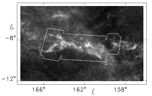
Figure 1: Extinction image of Dobashi et al. (2005) with the outline of our covered area shown to illustrate that we have observed most of the high extinction parts of this cloud. The maximum extinction is A${}_{v}=4.5$ mag and the minimum is essentially zero. The image is oriented in Galactic coordinates and covers an area of 12^∘ (l) $\times$ 7.3^∘ (b).

The initial data reduction process is essentially the same as that used for several other star-forming clouds from the Gould Belt Survey, e.g. (Sadavoy et al., 2012; Peretto et al., 2012). The first step consists of reducing the Herschel data to level 1 products using the Herschel Interactive Processing Environment (HIPE) version 8.1.0 (Ott, 2010). Maps of the three sub-regions listed in Table 1 were obtained using Scanamorphos version 16 (Roussel, 2012) using the two perpendicular scanmaps to remove correlated noise such as low frequency drifts. The pixel scales for these maps were 3.2″, 5″, 6″, 10″, and 14″ respectively at 70 µm, 160 µm, 250 µm, 350 µm, and 500 µm. These individual maps are shown in Figures 2–6 (electronic edition only). We then used two different source extractor routines. The first was the getsources package (version 1.120526) (Men‘shchikov et al., 2012) that was developed to search for sources over a range of spatial scales and extracts sources simultaneously over multiple bands that have substantial differences in angular resolution. The second source extractor was the c2dphot package developed as part of the Spitzer Legacy c2d program (Harvey et al., 2006; Evans et al., 2007) which was designed to work with point-like and small extended sources up to roughly twice the beam size and was based on the earlier DOPHOT package (Schechter, Mateo, & Saha, 1993). In this paper, we make use mostly of the results from the c2dphot processing (shown in Table 8) since we are primarily addressing point-like and very compact sources (§3, 4) in addition to the very large scale structure (§5). Future publications will use the results of the getsources processing to investigate the medium-scale emission.

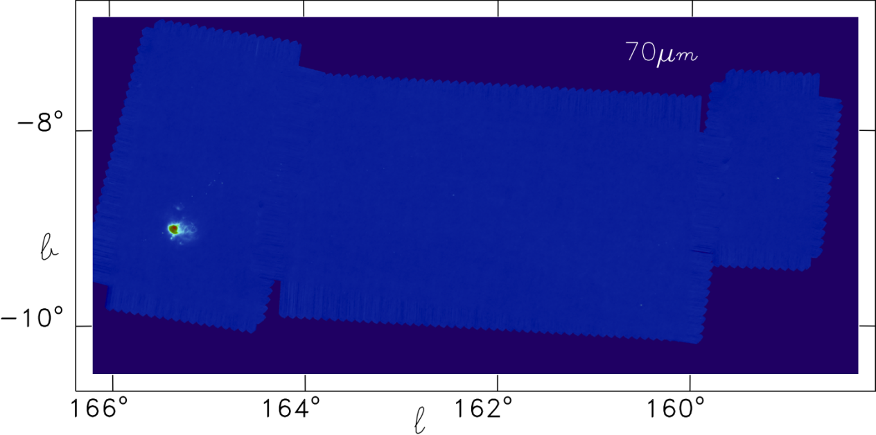
Figure 2: False color image of the 70 µm map derived with Scanamorphos from our Parallel-Mode observations.

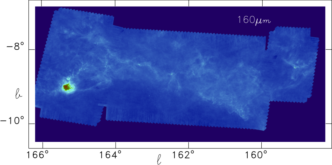
Figure 3: False color image of the 160 µm map derived with Scanamorphos from our Parallel-Mode observations.

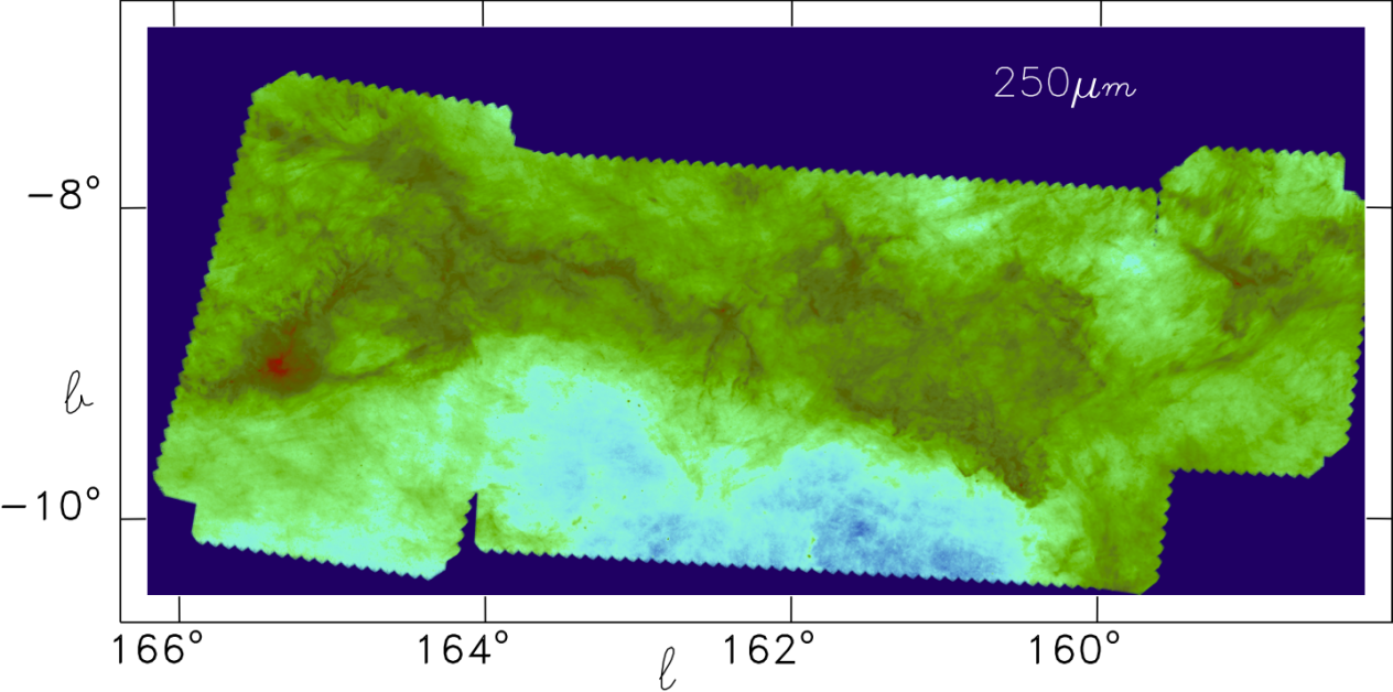
Figure 4: False color image of the 250 µm map derived with Scanamorphos from our Parallel-Mode observations.

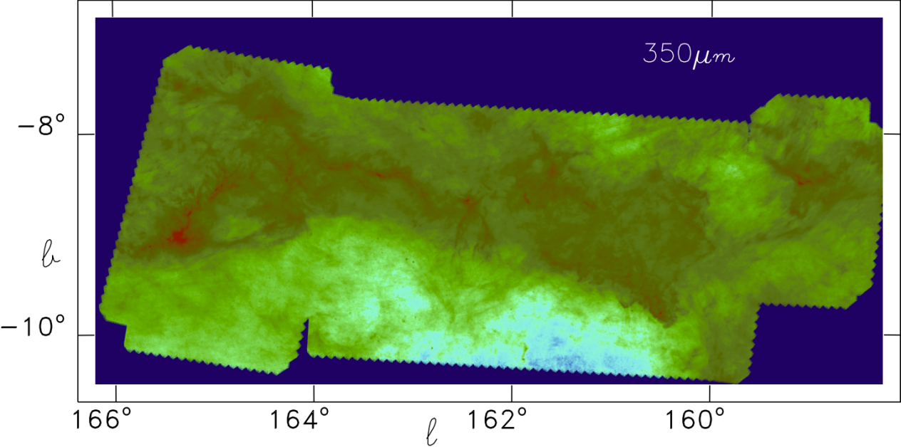
Figure 5: False color image of the 350 µm map derived with Scanamorphos from our Parallel-Mode observations.

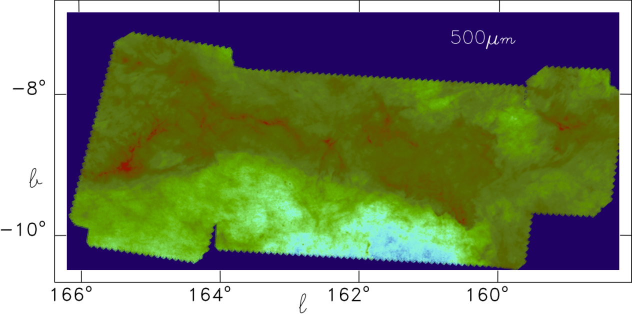
Figure 6: False color image of the 500 µm map derived with Scanamorphos from our Parallel-Mode observations.

Figure 7 shows a 3-color composite (70 µm, 160 µm, and 250 µm) of the entire region mapped at 70 µm, 160 µm, 250 µm, 350 µm, and 500 µm. The two most obvious features of this map are: 1) the bright collection of sources and nebulosity at the left end of the map (Southeast) where the LkH$\alpha$101 cluster is located, and 2) the long network of filamentary structure that pervades much of the mapped area. Such filamentary structure is now known to be typical in Galactic star-forming regions from the work of the Herschel Gould Belt survey (André et al., 2010) as well as the Herschel Galactic Plane Survey, HIGAL (Molinari et al., 2010) and has also been discussed earlier by Myers (2009). Subsections of some of the mapped areas are discussed in more detail later in §4.

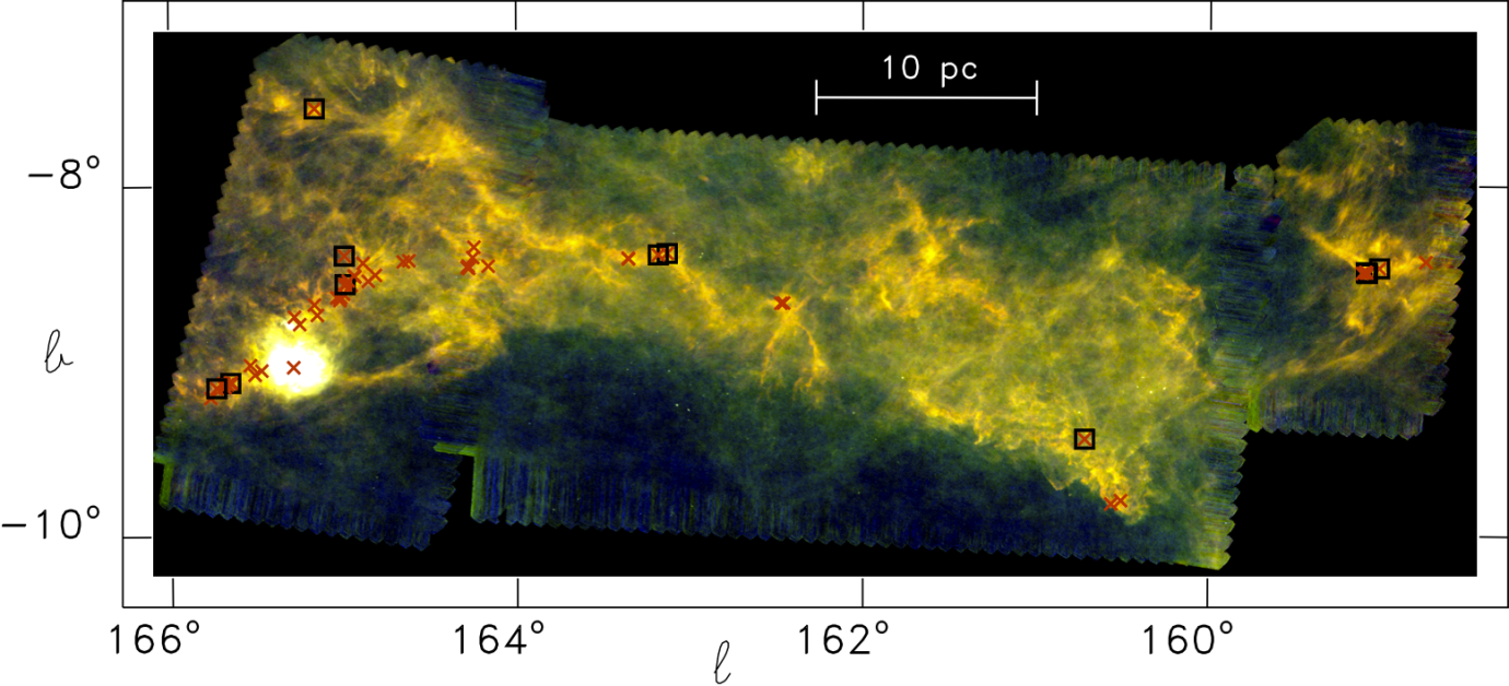
Figure 7: False color image with 70 µm (blue), 160 µm (green), and 250 µm (red) of the mapped area. The locations of the sources in Table 8 are marked with a red ‘X’, and those that are not in the Spitzer YSO list of H. Broekhoven-Fiene et al. (2013, in preparation) are also surrounded with a black square.

In addition to the basic map-making and source extraction, we also present in Figure 8 results on dust temperature and optical depth over the entire mapped area. We used a method similar to that described by Könyves et al. (2010); we first determined zero-point offsets following the procedure described by Bernard et al. (2010) and then convolved the shorter wavelength Herschel images to the resolution of the 500 µm data. We derived SED fits to the 160 $\mu$m, 250 $\mu$m, 350 $\mu$m, and 500 $\mu$m data for each pixel position in the maps using a simplified model of dust emission, $F_{\nu}=\kappa_{\nu}\times B(\nu,T)\times$ column density. We assumed a dust opacity law of $\kappa_{\nu}=0.1(\nu/1000GHz)^{\beta}cm^{2}/g)$ and fixed the dust emissivity index to $\beta$=2 with the standard mean molecular weight, $\mu$ = 2.33. Because of the high S/N over most of the area of the flux maps that were used to derive these column-density and temperature maps, the major uncertainty in the absolute values of T and $\tau$ are those due to the inherent assumptions in using the equations above to represent the dust emission. It is likely, though, that the maps provide an excellent representation of relative temperatures and column densities with absolute uncertainties of order $\pm$ 15–20% in temperature and $\pm$ a factor of 2 or more in column density. We discuss these maps more fully in §5 where we compare the column densities to those derived from extinction measurements and analyze the distribution of star formation relative to the inferred gas densities (note, all column densities discussed in this paper are measured as $N_{H2}$).

The digital versions of all these maps will be available soon after publication of this paper on the Herschel Science Center’s web site for user-provided data,

http://herschel.esac.esa.int/UserProvidedDataProducts.shtml.

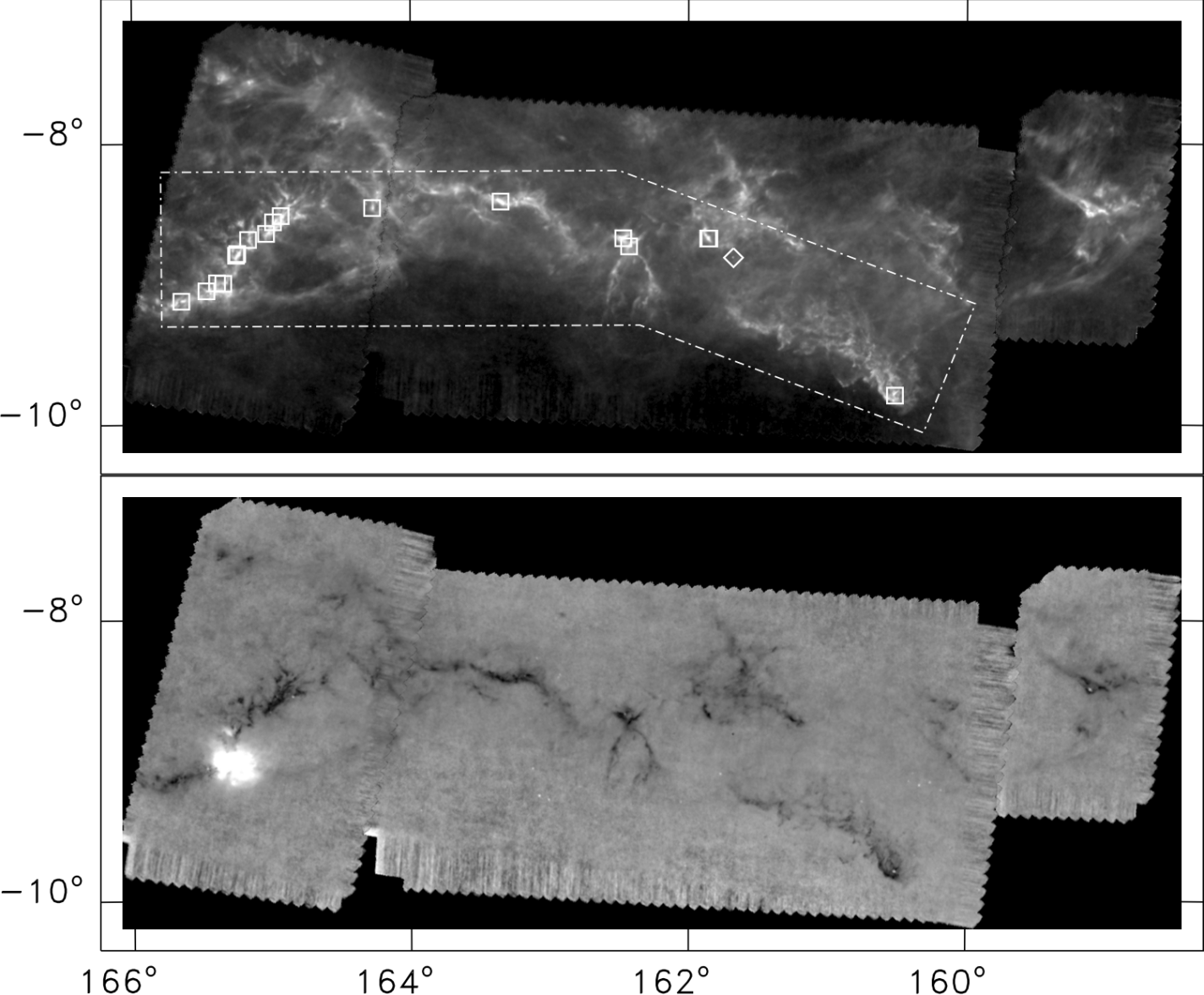
Figure 8: Upper image: column density image with positions of Bolocam 1.1 mm sources marked with squares (3C111 is indicated with the diamond). The area covered by our 1.1 mm Bolocam mapping is outlined with the dash-dot line. The highest column areas (white) have N${}_{H2}\sim 5\times 10^{22}$ cm^-2 while the lowest column areas represent values $\sim 1\times 10^{21}$ cm^-2. Lower image: dust temperature image with maximum T${}_{d}\sim$ 28K at LkH$\alpha$101 near the left end of the image and minimum temperatures of order 10K in the darkest parts of the filaments. The median derived dust temperature over most of the area is $\sim$ 14.5 K.

2.2 CSO Observations

We used the Bolocam imager at a wavelength of 1.1 mm to map much of the area covered in our Herschel observations during the nights of 14–16 November 2011. We utilized observing techniques similar to those used for the Bolocam Galactic Plane Survey (BGPS) as described by Aguirre et al. (2010) and Ginsburg et al. (in prep.). Alternating maps were made scanning roughly parallel and perpendicular to the Galactic plane at a scan speed of 120″s^-1. Multiple overlapping maps were obtained over roughly the eastern 2/3 of the Herschel mapped area; the total area observed was 6 deg²; the area covered is indicated in Figure 8. Due to non-uniform coverage and varying weather conditions the noise in the Bolocam maps is not constant, but is typically $\sim$ 0.07 Jy/beam. This is substantially higher than the noise in maps of several other Gould Belt clouds presented by Enoch et al. (2007), 0.01–0.03 Jy/beam, due to our significantly smaller observing time per pixel. The primary flux calibrator was Uranus. The map data were reduced using the software described by Aguirre et al. (2010) for the Bolocam Galactic Plane Survey (BGPS), utilizing correlated sky-noise reduction with 3 PCA (Principal Component Analysis) components. Following that, sources were extracted as described by Rosolowsky et al. (2010) for the BGPS. In addition to this large-scale mapping, we also observed a small area centered on one of the strong Spitzer sources to the northwest of the scanned region, SSTGB04012455+4101490, for which we have no corresponding Herschel data.

Aguirre et al. (2010) have carefully investigated the inherent spatial filtering that occurs in removing correlated sky-noise in ground-based observations at this wavelength. For the case of subtraction of 3 PCA components roughly half the flux is lost for structure larger than 300″. Indeed, the largest coherent area of 1.1 mm emission in our map is a 4′ wide area centered on LkH$\alpha$101. Therefore, we present the results from this part of the study as positions and flux densities for the compact emission regions detected. Table 8 lists these positions and the fluxes within several different apertures for the compact sources detected at 1.1 mm with peak S/N $>$ 2. Note, Source 2 is the bright galaxy 3C111 which was also our primary pointing calibrator and secondary flux calibrator. Table 8 also lists the Herschel sources from Table 8 that are located within 45″ of each 1.1 mm source position and likely associated with it. We discuss these 1.1 mm sources below in §3.2.

3 Compact Sources

3.1 The 70 µm Objects

The goal of our investigation of the compact sources in the AMC is to complete the search for pre-main-sequence and proto-stars that began with the Spitzer Gould Belt program (H. Broekhoven-Fiene et al. 2013, in preparation) and, in particular, to search for the most dust-enshrouded objects that might have been missed by that program because they emit most of their luminosity in the far-IR. Herschel at 70 µm provides the highest resolution imaging in the far-IR of any current or planned facility, and conveniently the 70 µm resolution ($\lambda/D\sim$ 4″) is also nearly identical to that of Spitzer at 24 µm. Although the resolution of Parallel-Mode observations is not quite as high as Herschel’s diffraction limit because of image blur from the fast scan speed in Parallel-Mode, the resolution achieved is not much below that limit. Therefore, an additional goal of this investigation is to use this resolution to measure fluxes in the far-infrared more reliably than Spitzer in confused regions. With a complete and reliable census of all the stages of star-formation in the AMC, we will be able to make the most informative comparison of it with the OMC.

The source extractor c2dphot operates in two modes. In the first mode, it searches through the image at sequentially lower flux levels for local maxima, characterizes them as point-like or extended (ellipsoidal), and subtracts them from the image. In the second mode the code is given a list of fixed positions at which it fits the point-source-function (PSF) to whatever flux above the background exists at that position. This mode is useful for determining upper limits and for testing for faint objects in the wings of bright ones. In both modes an aperture flux is calculated as well as the PSF- or ellipsoidal shape-derived flux. To find the most complete set of possible objects to correlate with objects at other wavelengths, we first processed both the 70 µm and 160 µm images in the most general c2dphot mode, allowing the code to fit flux, position, and shape down to the lowest flux levels present in the image, i.e., essentially the noise level. This process produced a list of $\sim$6500 sources at 70 µm and $\sim$500 sources at 160 µm, of which probably over half are noise at both wavelengths. After comparing a number of individual cases while trying to correlate the 160 µm objects with those found at 70 µm, we identified two complicating issues. First, the obvious issue of the larger PSF at the longer wavelength meant that sometimes more than one 70 µm source would be within the 160 µm PSF. Second, because cooler, more extended dust is naturally detected at the longer wavelength, in some cases the 160 µm source equivalent to a nearly point-like 70 µm source would be extended and have an asymmetric shape, making an automated detection and association difficult. For these reasons we decided to determine the 160 µm fluxes (or limits in most cases) for the 70 µm detections by running c2dphot in its second, fixed-position mode at 160 µm, using the 70 µm detection list for the input positions. In this case it can also be useful to compare the PSF-fit fluxes with those determined from aperture photometry as a secondary indication of larger source extent or confusion. For the six coldest sources discussed later in Figure 14 with T${}_{bol}<$ 40K we have also extracted flux densities at 250 µm in the same way as the 160 µm fluxes and show the PSF-fit fluxes. Since the 250 µm PSF has a full-width-half-maximum of roughly 18″, we have not measured the fluxes of the bulk of our objects beyond 160 µm; the issues with assigning fluxes to individual sources at 160 µm are incrementally more problematic at the SPIRE wavelengths. A future study making use of the getsources processing is likely to produce the most reliable long wavelength SEDs for most of the sources.

The nominal absolute calibration uncertainty in PACS photometry is now believed to be $\pm$3 % at 70µm and $\pm$ 5% at 160µm. These values only apply to well-sampled, color-corrected point sources. The SPIRE photometry is believed to be calibrated to $\pm$ 5% under equally ideal circumstances. For the purposes of this study, we assume the more conservative value of $\pm$ 15% as used, for example, by Könyves et al. (2010) from the original instrument papers by Poglitsch et al. (2010) and Griffin et al. (2010). Given that we have flux measurements for a number of sources at 70 µm also from the Spitzer Gould Belt program as well as flux determinations from our Herschel data set using the completely different getsources algorithm, we have an opportunity to check our flux measurements for systematic effects and problems like non-linearity. Figure 9 shows plots of these two comparisons. For the Spitzer comparison we used the list of reliable YSOs described by H. Broekhoven-Fiene et al. (2013, in preparation) and excluded several objects in very confused regions. The Spitzer photometry was produced by the version of c2dphot described in detail by Evans et al. (2007) for the final delivery of c2d data to the Spitzer Science Center. For the best getsources comparison (red diamonds in Figure 9) we used only sources found to be isolated, well-fit by a point source at 70 µm, with a product of major axis and minor axis less than 150″², a total flux less than $1.5\times$ the point-source flux, and a $S/N>10$. The mean ratio of Herschel to Spitzer fluxes is 1.03$\pm$0.3, and the mean ratio of c2dphot fluxes to getsources fluxes is 0.96$\pm$0.13 for the sources marked with red diamonds. The scatter between the Herschel and Spitzer results appears to be independent of flux level, while that between the two methods used on the Herschel data is consistent with what one would expect as a function of the signal-to-noise level. This excellent agreement, particularly for the two methods used on the Herschel data, between flux determinations over a very wide range of brightness suggests that both c2dphot and getsources provide highly reliable extractions and flux determinations, certainly for compact objects.

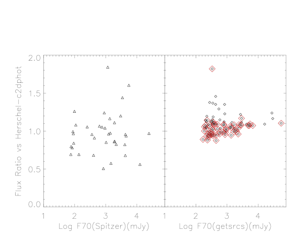
Figure 9: Comparison of 70 µm fluxes (mJy) derived in this study. Left panel: ratio of the fluxes from the Spitzer Gould Belt survey to the Herschel c2dphot fluxes from this study for the YSOs in common. Right panel: ratio of the fluxes using the getsources algorithm with our Herschel maps to those from our c2dphot processing for the high S/N objects found not to be extended on the basis of the quality of fit or derived source size. Those marked with red diamonds also included a criterion on ratio of total flux to PSF-fit flux being less than 1.5.

To identify the objects in the AMC that are most likely to represent young sources with a stellar or pre-main-sequence core, we culled our starting list of $\sim$ 6500 sources in several ways using shorter wavelength data. Much of our observed area has been covered at 24 µm in the Spitzer Gould Belt survey of H. Broekhoven-Fiene et al. (2013, in preparation); in areas not observed with Spitzer the recently released WISE all sky survey (Wright et al., 2010) provides relatively deep mid-infrared photometry over a similar range of wavelengths. To start our search for reliable young objects we included only those sources with S/N $>7.5$ and $F_{\nu}$ at 70 µm$>$ 85 mJy with at least a $2.5\sigma$ detection at one of the closest neighboring wavelengths, i.e. 22/24 µm Spitzer-MIPS/WISE, or our 160 µm Herschel photometry. These criteria reduced the list of possible young objects to 513 sources. Koenig et al. (2012) have estimated a contamination rate for extragalactic sources in star-forming regions at the sensitivity and wavelength of the WISE survey of $\sim$ 10 objects per square degree. This high background level suggests that a significant fraction of our 513 candidate sources is extragalactic.

To eliminate as many extragalactic sources from the candidate list as possible, we used a multi-pronged approach that relied on: (1) examination of individual images for likely galaxies at 70 µm as well as 24 µm (Spitzer), 2MASS, and the red (DSS) Digitized Sky Survey images, (2) Spitzer/WISE color-color diagrams using the criteria developed by Koenig et al. (2012), (3) the 2MASS “gal_contam” flag which signifies a likely extended extragalactic object (gal_contam = 1), and (4) objects of low S/N in the images or those that had no clear point-like core at 70 µm. Because of the wide range in colors, brightnesses, and angular sizes of the extragalactic objects, all of these criteria contributed substantially to the elimination process. After this triage we were left with 209 possible young candidates. This sample was clearly still “polluted” with extragalactic sources and evolved stars as we found by searching the SIMBAD data base and examining several dozen sources in DSS images. The most likely YSO candidates found by Spitzer (H. Broekhoven-Fiene et al. 2013, in preparation), however, are located exclusively in the areas of high column density illustrated in Figure 8, as are the 1.1 mm sources found in our Bolocam survey. Most of our 209 70 µm candidate young objects, though, are distributed quite uniformly over the area, as were the previously culled extragalactic objects and candidates. Therefore, at the risk of missing a likely very small number of young objects outside the high-column-density areas, we decided to apply one more criterion to our search list, i.e., to require the column density, as measured by Herschel at the 35″ resolution of the column density map, to be above 5 $\times 10^{21}$ cm^-2 (N_H2) at the source position. This threshold reduced the young candidate list to 60 objects. To be confident that this criterion did not eliminate any cold, dense young sources, we examined the DSS and 2MASS images of the few objects in lower column density regions that had $F_{160}/F_{70}>1.5$ and $F_{70}>150$ mJy, and all appeared extragalactic, i.e. not point sources. Therefore, the only young objects that we may have missed would be relatively faint and blue. Indeed, within the sample of Spitzer YSOs (H. Broekhoven-Fiene et al. 2013, in preparation) only one out of the $\sim$60 objects in the Class I–II range lies outside the N${}_{H2}\geq 5\times 10^{21}$ cm^-2 area of our column density map. The combination of all of the above criteria for eliminating extragalactic objects was important in reaching our final sample; for example, if we had simply applied the column density criterion alone, we would have extracted a sample of $\sim$ 120 objects, half of which obviously would have been background extragalactic sources behind higher column density local material. As an example of the contamination issue from extragalactic objects, Figure 10 shows a small field in the filament north of LkH$\alpha$101 with 6 YSOs identified by H. Broekhoven-Fiene et al. (2013, in preparation) (squares) and 4 objects identified as extragalactic from the 2MASS “gal_contam” flag (diamonds) that are also extended when examined carefully at 70 µm.

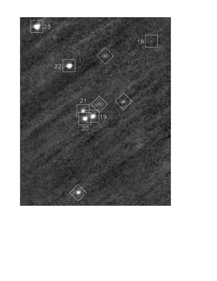
Figure 10: Field (10′ $\times$ 13′) centered at J2000 R.A. 04^h 28^m 33^s, decl. +36^∘ 25′ 20″ with 6 sources marked on the 70 µm image from Table 8 with squares and their source number, and 4 objects with diamonds identified as extragalactic using the 2MASS “gal_contam” flag. Orientation is North-up, East-left.

Table 8 lists the positions and 70 µm/160 µm c2dphot flux determinations of the final list of 60 objects found at 70 µm that appear to be reliable young members of the AMC. The uncertainties listed are the statistical uncertainties of the measurements only; the absolute calibration uncertainties of $\pm$15% have already been mentioned. For those sources that are identified also in the Spitzer Gould Belt data set, the 24 µm Spitzer flux is given, and if that is not available, the 22 µm WISE (Wright et al., 2010) flux is listed if available. The objects that are identified as YSO candidates by H. Broekhoven-Fiene et al. (2013, in preparation) are indicated, and where possible we list the object type shown by SIMBAD. Note, we think it unlikely that the 4 objects listed as “PN?” are truly evolved objects based on both their photometry and location in the AMC cloud. Table 8 also lists the spectral slope $\alpha$ ($\alpha={dlog(\lambda F(\lambda))\over dlog(\lambda)}$) determined from all existing members of the set of 3.6 µm, 24 µm, 70 µm, and 160 µm photometry; also shown is the corresponding YSO class based on the nomenclature of Lada (1987) as extended by Greene et al. (1994) as well as the total luminosity and the bolometric temperature as defined by Myers & Ladd (1993) determined over the same 3.6 µm–160 µm wavelength range. We have extended the classification to “Class 0” to signify the most dust-enshrouded objects as suggested by André et al. (1993). Since we do not have high angular resolution photometry for most of the objects at $\lambda\sim$ 1 mm, we have used the bolometric temperature to identify these objects within the nominal Class I category as defined by spectral slope. We used the criteria that objects with T${}_{bol}\leq$ 50 K are likely candidates for Class 0 objects, and those with 50 K $<$T${}_{bol}\leq$ 70 K we have marked as Class I/0, since some of them are likely to be identified as Class 0 when the requisite submillimeter photometry exists and reliable submillimeter to bolometric luminosity ratios can be derived. The class determinations are generally similar to those found for the YSO candidates of H. Broekhoven-Fiene et al. (2013, in preparation), though the addition of our more reliable 70 µm and 160 µm photometry has made changes for a few.

H. Broekhoven-Fiene et al. (2013, in preparation) report a total of 164 YSO candidates based on Spitzer and WISE photometry at $\lambda\leq$ 24µm within the area covered by our Herschel survey. Clearly a significant number of these are not detected in our study. We have examined this list of non-detections and find that most of them are simply too faint and blue to be likely to be detected in the far-infrared at our sensitivity level. Several redder and brighter Spitzer YSO candidates lie within the confused region around LkH$\alpha$101.

There are 11 objects in Table 8 that are not in the Spitzer YSO candidate lists of H. Broekhoven-Fiene et al. (2013, in preparation). Two of these (Sources 4 and 42) are completely undetected at 22/24 µm by WISE/Spitzer. We were able, however, to derive rough upper limits from the existing MIPS 24 µm images of 2 mJy for source 4 and 3 mJy for Source 42. Clearly both these objects exhibit relatively cold spectral energy distributions (SEDs). Most of the remaining 9 objects not found as YSO candidates by H. Broekhoven-Fiene et al. (2013, in preparation) were not selected by them simply because at least one IRAC or WISE band was missing from the detection list making classification as a YSO impossible using the Spitzer c2d/GB criteria. One of the 11 objects not identified previously as a YSO is Source 49 which has a very blue SED in the IRAC bands, but very strong far-infrared emission. It is one of only 6 objects with $T_{bol}<$ 40K (see also Figure 13 and §4).

3.2 The Bolocam Sources

Figure 8 shows the location of the 18 1.1 mm sources from Table 8 that are within our Herschel area relative to the column density derived from our Herschel mapping. With the exception of the galaxy 3C111 all of the 1.1 mm peaks fall on filaments of high column density. Excluding 3C111 and LkH$\alpha$101, $3/4$ of the 1.1 mm sources have Herschel 70 µm objects associated with them, and these are generally from the two “earliest” YSO classes, 0 and I (Note: Bolocam source 1 is associated with 70 µm source 9, which is a very bright emission-line star that is a likely FU Orionis object (Sandell & Aspin, 1998)). There are, however, four 1.1 mm emission sources with no associated Herschel source from Table 8. Source 10 is associated with a diffuse “blob” of emission near LkH$\alpha$101 in our 70 µm map, but Sources 3, 4, and 5 have no clear 70 µm counterpart. They are also three of the 1.1 mm sources with the lowest S/N ratio, but as just noted, they are clearly located on high-column-density filaments.

If the bulk of the 1.1 mm emission from the sources in Table 8 arises from very cool, dense, dust, then we might expect a correlation between the 1.1 mm flux density and the total Herschel-derived dust column density at that point, or more likely, the product of the Herschel-derived column density and temperature. This correlation would likely exist whether the dust is heated internally by a compact pre-main-sequence object or externally by the interstellar radiation field. To test this idea we have plotted in Figure 11 the 1.1 mm flux in an 80″ aperture versus the product of the Herschel-derived column density and temperature at the position of the 1.1 mm source, averaged over 80″. We have not included the galaxy 3C111 nor the hot, luminous source associated with LkH$\alpha$101 whose core dust temperature is unlikely to be well-sampled with the Herschel beams and whose flux levels are saturated at several Herschel wavelengths. Figure 11 shows a rather good correlation between 1.1 mm flux and the product of the Herschel-derived dust column density and temperature for all the other 1.1 mm sources. Thus, the three 1.1 mm sources without associated compact 70 µm sources probably deserve future investigation as possible pre-stellar cores.

Figure 11: Plot of 1.1 mm flux density in an 80″ aperture from Table 8 versus product of Herschel dust temperature and column density averaged over the same size aperture. LkH$\alpha$101 and 3C111 are not included. The correlation coefficient for this distribution is 0.67. The formal uncertainties in the product of dust temperature and column density are insignificant in comparison to the uncertainties due to the particular model used.

4 Individual Sources

There are several regions within our Herschel maps that are notable for either the number of young objects or strong emission at the longer wavelengths. H. Broekhoven-Fiene et al. (2013, in preparation) note the large number of Spitzer YSO candidates near LkH$\alpha$101 and in the filament extending north and west of it by roughly 1 degree. Figure 12 shows a 3-color composite image of this area with the positions of the Herschel sources from Table 8 marked. Roughly 60% of the likely young far-infrared sources listed in Table 8 are within a 1.2^∘ $\times$ 0.5^∘ area (9.4 pc $\times$ 3.9 pc) centered on the high-column-density filament shown in this area in Figure 8. The YSO population in the roughly 4′ $\times$ 4′ core of this region (0.5 pc square) centered on LkH$\alpha$101 has been summarized by Herbig et al. (2004) and Andrews & Wolk (2008). More recently Gutermuth et al. (2009) discussed Spitzer observations of this cluster in comparison with a number of other young clusters and Wolk et al. (2010) have added x-ray data to further define the cluster properties. Our Herschel observations are complementary to these studies in that the central few arcminutes of our images are dominated by the diffuse dust emission, presumably heated by the central bright star as well as the dense population of lower luminosity stars surrounding it. Beyond a radius of $\sim$ 3′ from LkH$\alpha$101, though, we are sensitive to compact thermal emission from individual members of the extended YSO population.

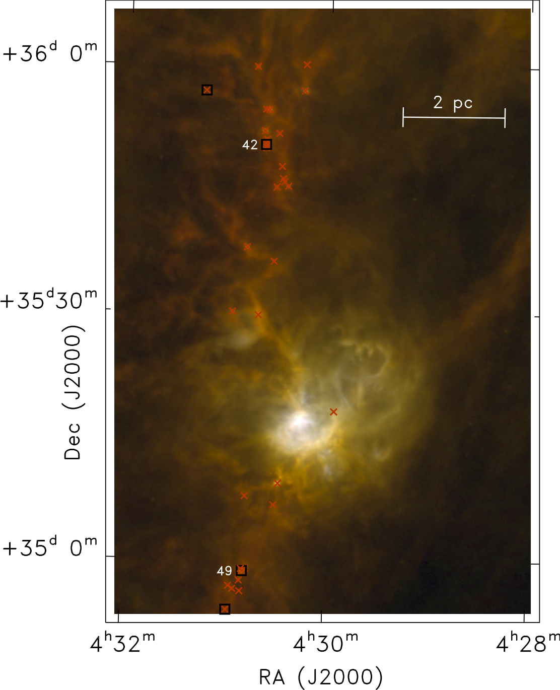
Figure 12: False color image with 70 µm (blue), 160 µm (green), and 250 µm (red) of the LkH$\alpha$101 area and star-forming filament to its north. As for Figure 7, the locations of the sources in Table 8 are marked with a red ‘X’, and those that are not in the Spitzer YSO list of H. Broekhoven-Fiene et al. (2013, in preparation) are also surrounded with a black square. LkH$\alpha$101 is the brightest object in the image. The second black square down from the northern boundary of the image is the location of Source 42, shown in more detail in Figure 13. The black square at the bottom of the image marks Source 49, also shown in more detail in Figure 13.

At the southern end of the filament containing LkH$\alpha$101 is a group of sources that includes Source 49, mentioned earlier as one of the objects with a very low T_bol in spite of being detected easily by Spitzer’s IRAC in all four bands with relatively blue colors. It also is extended in the IRAC images on a scale of $\sim$2–3″ in the north-south direction. These characteristics are consistent with it being a disk viewed edge-on, where the IRAC emission arises from scattered light above and below the plane of the disk along low extinction lines of sight to the central star; other interpretations are, of course, also possible. An expanded view of this source along with six other objects is shown in Figure 13a. The derived column density in this area peaks at $4\times 10^{22}$ cm^-2 essentially at the position of Source 49, and this area is associated with Bolocam Source 18. The SEDs of Source 49 and several other of the coldest sources discussed below are shown in Figure 14. As mentioned earlier, for these six examples of the coldest source SEDs we have extracted approximate PSF-fit fluxes at 250µm which show that the SEDs of all of these objects peak shortward of 250µm. Therefore, we have not found any compact objects with extremely cold SED’s, although this may be related to our requirement for detectable 70µm emission.

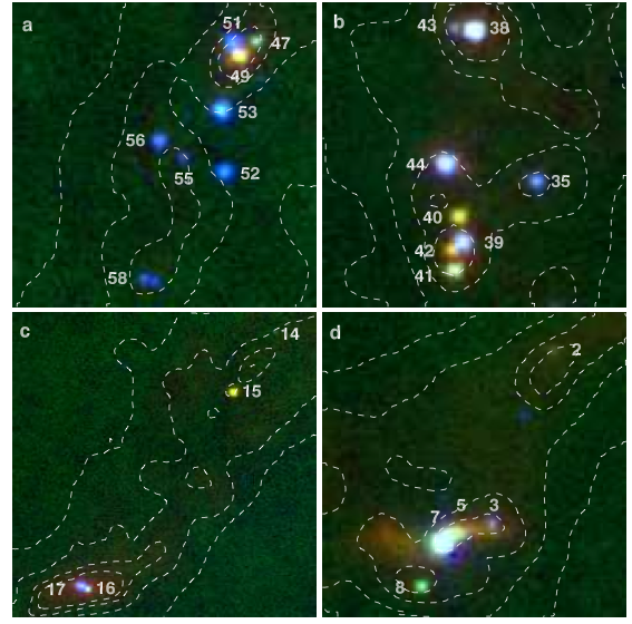
Figure 13: False color images of the four areas discussed in §4 with 24 µm (blue), 70 µm (green), and 160 µm (red). The sources are labeled with their reference numbers from Table 8 (for clarity, sources 4 and 6 are not marked in Panel d). Column density contours from the map shown in Figure 8 are overlaid at values of 0.5, 1.0, 2.0, and 3.0 $\times\ 10^{22}$ cm^-2 ($N_{H2}$). Panels a–d respectively have angular sizes of 6.4′, 5.9′, 12.8′, and 6.9′.

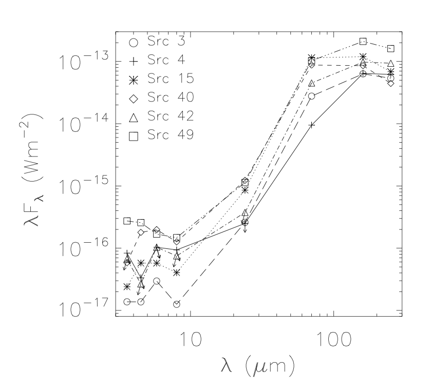
Figure 14: Spectral energy distributions of the six coldest sources discussed in §4. Note, sources 4 and 42 have only flux upper limits shortward of 70 µm.

Further north along the filament is a tight collection of young objects that includes one of our two 70 µm sources that was undetected by both Spitzer and WISE in the mid-infrared, Source 42 in Table 8 with spectral slope $\alpha\sim 3$ and also associated with Bolocam 1.1 mm Source 14. A closeup of this region is shown in Figure 13b. The image also includes 70 µm Sources 35, 38, 39, 40, 41, 43, and 44.

More than a degree northwest of the filament containing LkH$\alpha$101 is another region of high column density containing four objects from Table 8, Sources 14 – 17. Source 16 is a pointlike Class I/0 object located $\sim$ 16″ west of Source 17 (Class II), the latter of which is elongated in the direction of Source 16. Both are also associated with Bolocam Source 7, the third brightest 1.1 mm emission region. These two objects are shown in the lower left of Figure 13c. In the upper right are Source 15, another very cold object with spectral slope $\alpha\sim 3$, and Source 14, a faint Class I object.

Finally, in Figure 13d we show a tight collection of 7 Class 0 and I sources at the northwest end of our mapped area. These sources include an extended object at Herschel wavelengths that has been extracted as five separate condensations at 70 µm (Sources 3–7), three of which are well isolated Spitzer YSOs from H. Broekhoven-Fiene et al. (2013, in preparation). At 160 µm, however, the five sources are blended into a single elongated structure that peaks on the position of the brightest source at 24 µm, 70 µm, and 160 µm. Sources 2 and 8 from Table 8 are also included in this figure.

5 Cloud Mass and Structure

We have performed a preliminary analysis of the diffuse dust emission as described earlier by fitting the 160 µm–500 µm emission with a simple SED that characterizes the dust with a temperature and column density. These results shown in Figure 8 reveal a network of narrow filaments characterized by column densities of up to a few $\times\ 10^{22}$ cm^-2 ($N_{H2}$) and temperatures that drop to $\sim$ 10 K from the typical value of order 14–15K in the low-density parts of our maps. Many of these filaments are associated with Lynds dark clouds as indicated in Figure 1 of Lada, Lombardi & Alves (2009). In an initial effort to quantify the differences and similarities between the AMC and other star-forming regions we have calculated two quantities discussed by other authors for similar clouds. These quantities are the cumulative mass fraction as a function of extinction as already mentioned by Lada, Lombardi & Alves (2009) for the AMC and the probability density function for the column density as discussed by Schneider et al. (2012) and others.

Figure 15 shows the cumulative mass fraction versus K magnitude extinction A_K using the same conversion factors as Lada, Lombardi & Alves (2009), 2 $\times$ N_H2/A_K = 1.67 $\times$ 10²² cm^-2 mag^-1. The figure also shows the Lada et al. distribution as read from their Figure 4 and a version from our data after smoothing the Herschel-derived column density with an 80″ HPW Gaussian to try to duplicate the Lada et al. result. Both our native-resolution function as well as the smoothed version are well above the Lada et al. function at all values of A_K. It is possible that part of this difference is due to the fact that our observations cover only about half of the area mapped by Lada, Lombardi & Alves (2009) that has an extinction above A_K = 0.2 mag, though it is difficult to imagine quantitatively how such an areal difference could have such a large effect on the derived mass function. Another significant difference, besides just the basic technique, is the higher angular resolution of our data compared to the NICER optical extinction method, $\sim$ 35″ versus $\sim$ 80″, but our smoothed mass function is also well above that measured with the NICER technique. Yet another possible explanation for the difference is that there may exist a population of dust even colder than that sampled by the Herschel observations that could be contributing to the extinction-derived dust masses. The fact, however, that we have clearly sampled dust down to T$\sim$ 10 K and that the diffuse dust emission is significantly warmer at temperatures of order 14–15 K argues against this hypothesis. We have also investigated whether the difference might be due to differences in assumed dust properties. The underlying relationship which would affect Figure 15 is the ratio of far-ir optical depth used to derive our gas column density to the near-ir dust optical depth measured by Lada, Lombardi & Alves (2009). If, for example, the K-band extinction were smaller at any given value of far-ir optical depth, then the left side (low A_K) part of the Herschel-derived mass function would shift closer to that found by Lada, Lombardi & Alves (2009). On the other hand, however, the right side of our mass function (high A_K) would then drop far below the corresponding part of the NICER-derived mass function, particularly for the smoothed (80″) version of our mass function. Finally, it is also possible that the 2MASS-derived NICER extinctions do not sample well the highest column-density parts of the cloud. In any case, it will be very interesting to compare these results with Herschel-derived column density maps for the OMC to see if a similar discrepancy exists in that cloud between the NICER and SED-fitting methods.

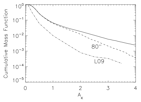
Figure 15: Normalized cumulative mass fraction for the area observed versus K magnitude extinction using the same assumptions as those of Lada, Lombardi & Alves (2009) (solid line). The dash-dot line shows the function derived by Lada, Lombardi & Alves (2009) with the NICER technique as read from their Figure 4, which is reported as smoothed with an 80″ HPW Gaussian. The dashed line shows the result of smoothing our Herschel-derived column density map with an 80″ HPW Gaussian.

The total mass in our mapped area is $\sim$ 4.9 $\times 10^{4}$ M_⊙ with 4.89 $\times 10^{4}$ M_⊙ above an extinction of A_K = 0.1 mag with the various assumptions mentioned earlier. As shown in Table 4, these mass values are about a factor of two below those found by Lada, Lombardi & Alves (2009) who observed a significantly larger area, most of which is occupied by relatively low column density material. So within the uncertainties the total masses are in reasonable agreement. Table 4 also illustrates numerically the difference in mass distribution in that our estimated mass above $A_{K}=1$ mag is three times larger than that found by Lada, Lombardi & Alves (2009) despite the smaller area covered in our study.

Figure 16 shows the probability density function (PDF) of column density for the AMC. This figure also shows three possible fits to portions of the PDF, two log-normal distributions for the central part of the PDF, and a power-law falloff for the high-extinction end for comparison with other recent studies of Gould Belt clouds. This observed distribution is qualitatively similar to other published column density PDFs, but peaks at a moderately lower column density, 2$\times$ 10²¹ cm^-2, than that for the Aquila region, 4 $\times$ 10²¹ cm^-2 (André et al., 2011). The power-law slope of -3 at high extinctions is comparable to that found for Aquila, as well as for the Rosette Nebula by Schneider et al. (2012).

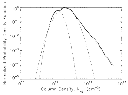
Figure 16: Normalized probability density function of area versus column density. The dashed line and dash-dot line show two different log-normal distributions that can fit portions of the PDF. The dotted line shows a power-law slope of -3.1 that roughly fits the extended tail of the distribution at high column densities.

Qualitatively Figure 16 supports the suggestion by Lada, Lombardi & Alves (2009) that the AMC has relatively less high-column-density material than more prolific star-forming regions like the Orion Molecular Cloud. This conclusion will be able to be further quantified as the Herschel data on the OMC become available for comparison, since it is clear already from our results that the resolution of the observations and technique used may be important to the detailed results. Further analysis will hopefully also provide some insight into the underlying physical mechanisms that lead to these differences.

5.1 Star Formation Versus Column Density

We have already discussed the fact that virtually all the young stellar objects are found along the high column density filamentary structure shown in Figure 8. In fact, if we confine our sample to the Class 0 through II SED objects that are likely to be young enough that they are still close to their birthplaces in the cloud, there is only one YSO outside the regions of the cloud with N${}_{H2}<5\times\ 10^{21}$ cm^-2 as mentioned earlier. We can investigate whether there is a quantitative as well as qualitative correlation by smoothing both distributions and comparing the YSO surface density with the gas surface density. Figure 17 shows the result of this comparison, where we plot the surface density of the 68 Class 0–II YSOs and the Herschel-derived gas column density, both smoothed with a 0.2^∘(1.6 pc) half-power-width Gaussian. For the YSOs we used the union of Spitzer (H. Broekhoven-Fiene et al. 2013, in preparation) and Herschel (this paper) objects. The two highest concentrations of YSOs are found in the LkH$\alpha$101 cluster and in a clump in the northern filament about 3/4^∘ north of LkH$\alpha$101. The derived column density is also highest in these two areas as smoothed to a 0.2^∘ half-power-width. There is, however, a less perfect correlation between YSO surface density and derived gas column density at the intermediate levels, but it is certainly true that the greatest number of YSOs are found in the regions with the highest concentration of dust and gas. Conversely, in lower column density areas, but still above the general background level, essentially no YSOs are found.

Kennicutt & Evans (2012) have reviewed this subject extensively in the context of both Galactic and extragalactic star formation. Likewise Lada, Lombardi & Alves (2010) and Heiderman et al. (2010) have attempted to compare star formation rates and gas surface densities in multiple local star-forming environments. All of these studies find a roughly power-law relation between gas density and star formation rate over some range of gas densities. We can quantify our own conclusions by computing the ratio of the two maps plotted in Figure 17 as a function of the derived column density. Figure 18 shows the average of this ratio in ten column density bins expressed as $A_{K}$ (mag) from the map smoothed with a 0.2^∘ Gaussian. This plot shows clearly that there is a strong power-law relationship between star formation and column density in the AMC. The surface density of young stellar objects increases rapidly at the highest column densities. The slope of this relationship is 4.0. This conclusion does not depend strongly on the details of our sample since the distribution of Spitzer and Herschel YSOs is similar within the small-number statistics, and our derived column density map is qualitatively similar to that of Dobashi et al. (2005). This slope of 4.0 is comparable to, but slightly less than the slope of 4.6 derived by Heiderman et al. (2010) for an ensemble of star-forming regions at comparable levels of extinction (surface density). We do not, however, see any obvious break point in the relation between YSO surface density and gas column density, though such a break point might be masked by the smoothing process necessary to deal with relatively small number of YSOs. Note also that our maximum smoothed extinction is A${}_{K}\sim 1.0$ mag, equivalent to a visual extinction of A${}_{V}\sim 8$ mag which is just below the level where Heiderman et al. (2010) see a break in their power-law slope.

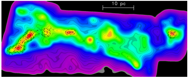
Figure 17: Derived $N_{H2}$ column density smoothed with a 0.2^∘ (HPW) Gaussian shown in colored contours versus the YSO surface density smoothed in the same way in black dash-dot contours. The YSO contours are in steps of 1, 2, 4, and 8 YSOs per smoothed beam for the Class 0–II objects. The smoothed column density ranges from 1 to 8.6 $\times 10^{21}$ cm^-2.

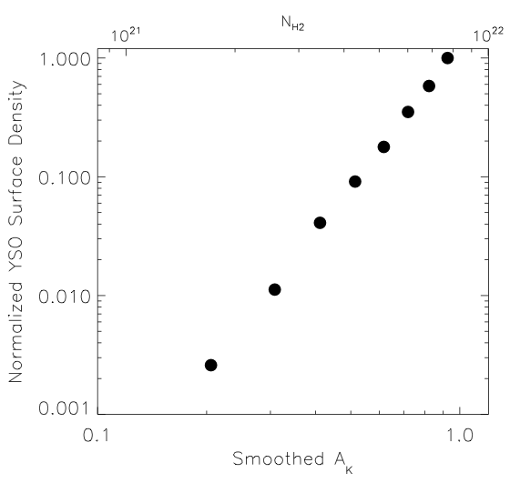
Figure 18: Plot of the ratio of smoothed YSO surface density to smoothed column density (normalized to the peak) relative to the smoothed column density (expressed in K magnitude extinction $A_{K}$), both from Figure 17.

5.2 Ionizing Environment

Sharp edges suggesting shaping by photoionization are seen along the southern border of the cloud (Fig. 7), particularly in the west near $\ell=160.5\arcdeg,{\it b}=-9.5$°, even down to low-column densities. The effects of photoionization, however, are modest because there is no evidence for a temperature gradient indicative of dust heating. The sharp cloud edges are reminiscent of the similar but stronger effects seen in the Oph North region (upper Scorpius) which is being photoionized and shaped by the runaway O star $\zeta$ Ophiuchi (Hatchell et al., 2012).

A possible source of photoionization is the O7.5 III star $\xi$ Per ($\ell=160.4\arcdeg,b=-13.1\arcdeg$). The star $\xi$ Per illuminates the California Nebula, a bright infrared nebula located between the star and the AMC in projection. Hoogerwerf et al. (2001) model $\xi$ Per as a runaway O star that was ejected from the Per OB2 association, and that now has a distance of 360 pc. The proper motion and distance uncertainties, however, are also consistent with the interpretation that $\xi$ Per is closer to the AMC cloud, and hence able to influence the AMC cloud boundary. In any case, the influence of $\xi$ Per on the structure of the AMC is minimal, and there is no indication of enhanced star formation along the southwest cloud boundary.

6 Comparison of the AMC and OMC

As mentioned above, a comparable Herschel study of the OMC is not yet complete so it is not possible yet to make a detailed comparison of the star formation and interstellar medium between the two giant molecular clouds in the far-infrared. We can, however, discuss briefly the differences in star formation rate on the basis of our deep Herschel observations. H. Broekhoven-Fiene et al. (2013, in preparation) have shown that on the basis of Spitzer searches for infrared-excess objects, the AMC appears to have about 5% of the YSO population over a similar area as that of the OMC (Megeath et al., 2012). Our Herschel photometry has discovered a few additional young objects on the basis of 70 µm and 160 µm fluxes, but there is clearly not a significant population of deeply buried YSOs. This ratio of 20:1 for the star formation rates is, though, not as great as the ratio of the incidence of very massive stars. For example, the seminal study of Blaauw (1964) found more than 50 O and early B stars in the Orion OB associations, whereas the AMC probably has only one early B star. This suggests that whatever the reasons for the lower star formation rate in the AMC despite its total mass, the rate for high mass stars is depressed even more in the AMC relative to that in the OMC.

7 Summary

We have completed the census of star formation in the AMC that began with the Spitzer Gould Belt survey of H. Broekhoven-Fiene et al. (2013, in preparation). We have found a modest number of additional YSOs, 11, several of which exhibit quite cold SEDs that peak at 150 µm-200µm. We also mapped a subsection of the Herschel area with Bolocam at 1.1 mm and found 18 cold dust sources whose fluxes are well correlated with the dust temperature and column density derived at shorter wavelengths with Herschel. We have analyzed the distribution of column density and found a strong non-linear relation between column density and YSO surface density. We have compared our derived cumulative mass fraction with that found by Lada, Lombardi & Alves (2009) with the NICER method and noted some differences that may be due to a combination of factors including: area covered, angular resolution, and details of the methods. The cumulative mass fraction and the probability density function for the column density are both qualitatively similar to other clouds for which they have been derived but may suggest that the AMC is dominated by lower column density material than other clouds with higher rates of star formation as suggested by Lada, Lombardi & Alves (2009). The star formation rate in the AMC appears to be a factor of 20 below that in the OMC for typical stars, but an even greater difference exists at the high-mass end of the IMF.

8 Acknowledgments

We thank Nicholas Chapman and Giles Novak for their help with the CSO/Bolocam observations, and we thank the anonymous referee who provided a number of comments that noticeably improved this paper. Support for this work, as part of the NASA Herschel Science Center data analysis funding program, was provided by NASA through a contract issued by the Jet Propulsion Laboratory, California Institute of Technology to the University of Texas. Partial support for T.L.B. was provided by NASA through contract 1433108 issued by the Jet Propulsion Laboratory, California Institute of Technology, to the Smithsonian Astronomical Observatory.

This publication makes use of data products from the Wide-field Infrared Survey Explorer, which is a joint project of the University of California, Los Angeles, and the Jet Propulsion Laboratory/California Institute of Technology, funded by the National Aeronautics and Space Administration. This research has also made use of the SIMBAD database, operated at CDS, Strasbourg, France.

Table 1: AOR List

AOR Name	ObsID	Field Center	Comments
SPParallel-aurwest-orth	1342239276	04 09 53.0 +39 59 30	Western End
SPParallel-aurwest-norm	1342239277	04 10 00.0 +40 01 27	Western End
SPParallel-aurcntr-orth	1342239278	04 18 57.0 +37 45 09	Central Region
SPParallel-aurcntr-norm	1342239279	04 19 03.5 +37 44 54	Central Region
PPhoto-secluster-orth	1342239441	04 30 30.0 +35 30 00	LkHa101 Cluster
PPhoto-secluster-norm	1342239442	04 30 30.0 +35 30 00	LkHa101 Cluster
SPParallel-aureast-orth	1342240279	04 30 20.7 +35 50 57	Eastern End
SPParallel-aureast-norm	1342240314	04 30 19.9 +37 50 58	Eastern End

Table 2: Herschel Source Fluxes And Derived Quantities

Src	YSO	SIMBAD	RA/Dec Center (J2000)	MIR	$\alpha$	YSO	Lbol	Tbol	Fν 22/24 µm	Fν 70 µm	Fν 70 µm	Fν 160 µm	Fν 160 µm
		Type	h m s  ∘ ′ ″			Class	L⊙	K	mJy	(PSF) mJy	(Aper) mJy	(PSF) mJy	(Aper) mJy
1	Y	IR	04 09 02.16 $+$40 19 11.4	WISE	0.56	I	2.16	152	980$\pm$ 91	3880$\pm$ 98	3950$\pm$ 120	3360$\pm$ 290	4600$\pm$ 110
2			04 09 54.71 $+$40 06 39.9	SpGB	0.99	I	0.11	71	7.16$\pm$0.70	144$\pm$ 7.6	185$\pm$ 27	818$\pm$ 92	2210$\pm$ 48
3	Y		04 10 02.81 $+$40 02 43.9	SpGB	2.37	0	0.37	31	2.08$\pm$0.68	647$\pm$ 26	583$\pm$ 36	3370$\pm$ 750	12600$\pm$ 92
4			04 10 04.53 $+$40 02 37.5	SpGB	1.78	0	0.29	28	$<$ 2.00	221$\pm$ 12	348$\pm$ 120	3430$\pm$ 690	18800$\pm$ 140
5	Y		04 10 05.88 $+$40 02 37.0	SpGB	1.04	0	0.61	42	3.51$\pm$0.68	592$\pm$ 46	989$\pm$ 590	6660$\pm$ 1800	31800$\pm$ 280
6		IR	04 10 07.08 $+$40 02 34.6	WISE	1.19	0	2.00	48	156$\pm$ 4.5	2230$\pm$ 110	4080$\pm$ 3000	18600$\pm$ 2700	54000$\pm$ 550
7	Y	IR	04 10 08.58 $+$40 02 23.2	SpGB	1.05	I	12.11	97	4770$\pm$ 470	25400$\pm$ 390	29000$\pm$ 660	33800$\pm$ 4400	58600$\pm$ 670
8	Y		04 10 11.29 $+$40 01 24.4	SpGB	1.94	0	0.55	47	41.1$\pm$ 3.8	1610$\pm$ 25	1550$\pm$ 59	2670$\pm$ 190	3850$\pm$ 89
9	Y	Em*	04 10 40.95 $+$38 07 52.4	WISE	0.32	I	40.53	239	15001$\pm$ 170	50100$\pm$ 1000	52800$\pm$ 1400	53000$\pm$ 4200	66600$\pm$ 1200
10	Y	Em*	04 10 49.03 $+$38 04 43.8	SpGB	-0.25	F	0.47	337	123$\pm$ 11	240$\pm$ 11	234$\pm$ 29	923$\pm$ 61	1860$\pm$ 47
11			04 12 40.54 $+$38 14 26.8	SpGB	0.96	I/0	0.02	65	0.83$\pm$0.20	82.9$\pm$ 9.0	$\cdots$	81.4$\pm$ 23	$\cdots$
12	Y	RNe	04 21 37.77 $+$37 34 41.1	SpGB	0.04	F	3.40	290	223$\pm$ 21	3450$\pm$ 94	4620$\pm$ 320	13900$\pm$ 930	25900$\pm$ 250
13	Y		04 21 40.58 $+$37 33 58.3	SpGB	0.94	I	0.56	123	241$\pm$ 23	910$\pm$ 27	906$\pm$ 44	1450$\pm$ 290	4170$\pm$ 62
14			04 24 59.04 $+$37 17 52.9	SpGB	0.84	I	0.04	93	7.63$\pm$0.73	138$\pm$ 11	117$\pm$ 30	98.9$\pm$ 38	112$\pm$ 41
15		IR	04 25 07.83 $+$37 15 19.3	SpGB	2.45	0	0.94	36	6.85$\pm$0.67	2670$\pm$ 48	2700$\pm$ 76	6360$\pm$ 620	8200$\pm$ 210
16	Y	IR	04 25 38.30 $+$37 06 59.2	SpGB	1.36	I/0	0.57	55	59.1$\pm$ 5.5	1160$\pm$ 29	1090$\pm$ 110	3490$\pm$ 400	9330$\pm$ 88
17	Y	IR	04 25 39.60 $+$37 07 06.5	SpGB	-0.61	II	2.95	459	727$\pm$ 68	630$\pm$ 15	637$\pm$ 190	1350$\pm$ 340	10100$\pm$ 89
18	Y		04 28 14.90 $+$36 30 27.4	SpGB	-0.27	F	0.13	296	61.3$\pm$ 5.7	109$\pm$ 14	$\cdots$	99.0$\pm$ 41	792$\pm$ 54
19	Y		04 28 35.07 $+$36 25 05.2	SpGB	0.49	I	0.91	158	237$\pm$ 22	1660$\pm$ 43	1590$\pm$ 57	2400$\pm$ 200	3590$\pm$ 69
20	Y		04 28 37.87 $+$36 24 54.9	SpGB	-0.23	F	1.20	338	204$\pm$ 19	1290$\pm$ 31	1230$\pm$ 53	1950$\pm$ 180	3620$\pm$ 65
21	Y	IR	04 28 38.54 $+$36 25 28.1	SpGB	0.94	I	0.34	83	143$\pm$ 13	723$\pm$ 21	704$\pm$ 38	1010$\pm$ 200	2750$\pm$ 56
22	Y		04 28 43.66 $+$36 28 37.6	SpGB	1.16	I/0	0.93	68	192$\pm$ 18	2630$\pm$ 73	2670$\pm$ 90	3150$\pm$ 290	4960$\pm$ 95
23	Y	IR	04 28 55.24 $+$36 31 21.6	SpGB	0.60	I	2.33	138	752$\pm$ 70	4490$\pm$ 140	4560$\pm$ 150	5870$\pm$ 720	9080$\pm$ 210
24	Y	IR	04 29 54.15 $+$36 11 56.3	WISE	-0.40	II	1.00	322	534$\pm$ 50	726$\pm$ 18	657$\pm$ 36	712$\pm$ 55	960$\pm$ 45
25	Y	Y*O	04 29 55.05 $+$35 18 04.8	SpGB	-0.22	F	0.43	268	135$\pm$ 13	669$\pm$ 77	1480$\pm$ 170	$\cdots$	4760$\pm$ 100
26	Y		04 29 59.31 $+$36 10 17.5	WISE	-0.34	II	0.12	434	10.6$\pm$ 1.0	88.8$\pm$ 11	58.0$\pm$ 34	207$\pm$ 51	689$\pm$ 42
27	Y		04 30 14.89 $+$36 00 08.3	SpGB	0.96	I	0.12	120	48.2$\pm$ 4.5	198$\pm$ 10	163$\pm$ 28	297$\pm$ 33	490$\pm$ 39
28	Y	PN?	04 30 15.68 $+$35 56 57.8	WISE	-0.46	II	19.21	368	8160$\pm$ 130	14900$\pm$ 420	15500$\pm$ 420	5510$\pm$ 900	10500$\pm$ 170
29	Y		04 30 24.58 $+$35 45 20.8	SpGB	0.51	I	2.88	150	1400$\pm$ 130	4840$\pm$ 100	4960$\pm$ 130	4830$\pm$ 210	5480$\pm$ 120
30	Y		04 30 26.91 $+$35 45 51.9	SpGB	0.39	I	0.08	117	14.4$\pm$ 1.4	179$\pm$ 7.2	173$\pm$ 37	243$\pm$ 57	1110$\pm$ 49
31	Y	Y*O	04 30 27.59 $+$35 09 17.5	SpGB	1.04	I	9.26	105	1580$\pm$ 160	22500$\pm$ 840	28100$\pm$ 520	32400$\pm$ 3000	45400$\pm$ 670
32	Y		04 30 27.71 $+$35 46 14.6	SpGB	-0.31	II	0.23	331	95.0$\pm$ 8.8	120$\pm$ 8.7	97.0$\pm$ 33	275$\pm$ 93	1220$\pm$ 45
33	Y		04 30 28.50 $+$35 47 44.5	SpGB	-0.36	II	0.18	395	33.4$\pm$ 3.1	96.6$\pm$ 9.9	70.7$\pm$ 29	262$\pm$ 39	624$\pm$ 40
34	Y		04 30 30.05 $+$35 06 39.9	SpGB	-0.44	II	0.13	356	38.5$\pm$ 3.7	117$\pm$ 11	162$\pm$ 35	133$\pm$ 77	627$\pm$ 41
35	Y		04 30 30.50 $+$35 51 44.1	SpGB	0.45	I	0.42	152	187$\pm$ 17	590$\pm$ 13	538$\pm$ 32	1050$\pm$ 77	1530$\pm$ 50
36	Y		04 30 31.53 $+$35 45 14.3	SpGB	-0.36	II	1.10	352	403$\pm$ 37	595$\pm$ 16	581$\pm$ 35	931$\pm$ 120	1830$\pm$ 54
37	Y	IR	04 30 32.32 $+$35 36 13.4	SpGB	0.07	F	0.72	149	292$\pm$ 27	1440$\pm$ 35	1250$\pm$ 57	1470$\pm$ 84	1720$\pm$ 52
38	Y		04 30 36.74 $+$35 54 36.8	SpGB	1.11	I	2.67	92	529$\pm$ 50	6280$\pm$ 160	6390$\pm$ 190	9750$\pm$ 870	13400$\pm$ 250
39	Y	TT?	04 30 37.42 $+$35 50 31.4	SpGB	-0.10	F	1.65	275	390$\pm$ 36	1720$\pm$ 33	1930$\pm$ 220	4140$\pm$ 600	13100$\pm$ 170
40	Y		04 30 37.81 $+$35 51 01.2	SpGB	2.10	0	0.72	38	9.82$\pm$0.92	2040$\pm$ 51	1940$\pm$ 83	4560$\pm$ 770	7070$\pm$ 160
41	Y		04 30 38.14 $+$35 49 59.5	SpGB	2.15	0	0.89	44	70.5$\pm$ 6.5	2190$\pm$ 47	2180$\pm$ 100	5270$\pm$ 550	10500$\pm$ 160
42			04 30 38.38 $+$35 50 22.6	SpGB	2.07	0	0.58	32	$<$ 3.00	1050$\pm$ 21	944$\pm$ 370	5210$\pm$ 1800	14500$\pm$ 180
43	Y	IR	04 30 38.76 $+$35 54 40.2	SpGB	0.21	F	0.23	201	53.4$\pm$ 4.9	263$\pm$ 12	$\cdots$	822$\pm$ 220	6870$\pm$ 160
44	Y	IR	04 30 39.18 $+$35 52 02.1	SpGB	-0.09	F	2.41	249	899$\pm$ 85	2510$\pm$ 71	2920$\pm$ 85	5070$\pm$ 600	9480$\pm$ 110
45	Y		04 30 41.13 $+$35 29 40.5	SpGB	1.18	I	0.93	81	176$\pm$ 16	2230$\pm$ 57	2310$\pm$ 70	3620$\pm$ 240	6480$\pm$ 98
46	Y	PN?	04 30 44.13 $+$35 59 50.8	SpGB	0.24	F	2.81	254	1270$\pm$ 120	2390$\pm$ 52	2170$\pm$ 73	3120$\pm$ 200	3860$\pm$ 88
47	Y		04 30 46.20 $+$34 58 55.6	SpGB	1.57	0	0.31	49	26.9$\pm$ 2.5	719$\pm$ 20	826$\pm$ 130	1840$\pm$ 240	10900$\pm$ 240
48	Y		04 30 47.24 $+$35 07 42.6	SpGB	-0.49	II	0.16	379	51.8$\pm$ 4.8	107$\pm$ 13	114$\pm$ 34	84.1$\pm$ 56	345$\pm$ 42
49		PN?	04 30 47.90 $+$34 58 37.3	SpGB	1.89	0	1.27	33	9.09$\pm$ 1.6	2400$\pm$ 49	2430$\pm$ 110	11200$\pm$ 1300	18700$\pm$ 340
50	Y	IR	04 30 48.42 $+$35 37 54.4	SpGB	1.01	I	1.92	92	452$\pm$ 42	5020$\pm$ 140	5160$\pm$ 150	5620$\pm$ 580	8220$\pm$ 170
51	Y	PN?	04 30 48.54 $+$34 58 52.7	SpGB	-0.20	F	0.79	236	677$\pm$ 63	466$\pm$ 26	618$\pm$ 370	623$\pm$ 450	15900$\pm$ 320
52	Y		04 30 49.18 $+$34 56 10.2	SpGB	-0.02	F	0.48	236	277$\pm$ 26	475$\pm$ 15	453$\pm$ 34	382$\pm$ 25	227$\pm$ 41
53	Y	Or*	04 30 49.63 $+$34 57 27.9	SpGB	-0.69	II	2.54	451	677$\pm$ 63	1210$\pm$ 42	1230$\pm$ 52	1240$\pm$ 220	1720$\pm$ 54
54	Y		04 30 52.00 $+$34 50 08.4	WISE	-0.26	F	0.31	322	114$\pm$ 11	253$\pm$ 9.9	316$\pm$ 33	364$\pm$ 50	223$\pm$ 44
55	Y		04 30 53.41 $+$34 56 26.4	SpGB	0.54	I	0.06	130	27.2$\pm$ 2.5	81.3$\pm$ 9.6	74.2$\pm$ 35	160$\pm$ 47	607$\pm$ 43
56	Y		04 30 55.92 $+$34 56 48.3	SpGB	0.54	I	0.25	134	141$\pm$ 13	377$\pm$ 12	385$\pm$ 38	503$\pm$ 59	1040$\pm$ 46
57	Y	IR	04 30 56.49 $+$35 30 04.5	SpGB	1.54	I	1.00	70	302$\pm$ 28	2560$\pm$ 86	2670$\pm$ 87	3180$\pm$ 460	5150$\pm$ 110
58			04 30 57.19 $+$34 53 53.6	WISE	0.38	I	0.11	175	39.9$\pm$ 3.7	129$\pm$ 10	133$\pm$ 30	353$\pm$ 53	1130$\pm$ 43
59			04 31 14.67 $+$35 56 50.6	SpGB	0.76	I	0.09	103	26.4$\pm$ 2.5	178$\pm$10	150$\pm$ 35	261$\pm$ 45	590$\pm$ 46
60			04 34 53.15 $+$36 23 27.9	WISE	-0.44	II	2.76	367	1089$\pm$ 15	1840$\pm$ 46	1810$\pm$ 61	1770$\pm$ 190	3140$\pm$ 77

Table 3: 1.1 mm Source Fluxes

Table 4: Cumulative Mass Versus Extinction

$A_{K}$ (mag)	Mass (this study)	Mass (Lada09)
Mag	M⊙	M⊙
0.0	4.9 $\times 10^{4}$	NA
0.1	4.89 $\times 10^{4}$	1.12 $\times 10^{5}$
0.2	4.28 $\times 10^{4}$	5.34 $\times 10^{4}$
1.0	3.29 $\times 10^{3}$	1.09 $\times 10^{3}$

References

- Aguirre et al. (2010) Aguirre, J.E., Ginsburg, A.G., Dunham, M.K., et al. 2010, ApJS, 192, 4
- André et al. (1993) André, P., Ward-Thompson, D. & Barsony, M. 1993, ApJ, 406, 122
- André et al. (2010) André, P., Men‘shchikov, A., Bontemps, S., et al. 2010, A&A, 518, L102
- André et al. (2011) André, P., Men‘shchikov, A., Konyves, V. & Arzoumanian, D. 2011, Computational Star Formation”, IAU Symposium, Volume 270, Eds. J. Alves, B. Elmegreen, V. Trimble, Cambridge University Press, p. 255
- Andrews & Wolk (2008) Andrews, S.M. & Wolk, S.J. 2008,in ASP Monograph Ser. 5, Handbook of Star Forming Regions, Vol. 2, The Southern Sky, ed. B. Reipurth (San Francisco, CA: ASP), 390
- Arzoumanian et al. (2011) Arzoumanian, D., André, Ph., Didelon, P., et al. 2011, A&A, 529, L6
- Bernard et al. (2010) Bernard, J.-Ph., Paradis, J., Marshall, D.J., et al. 2010, A&A, 518, L88
- Blaauw (1964) Blauuw, A. 1964, ARA&A, 2, 213
- Dame et al. (2001) Dame, T.M., Hartmann, D. & Thaddeus, P. 2001, ApJ, 547, 792
- Dobashi et al. (2005) Dobashi, K., Uehara, H., Kandori, R., et al. 2005, PASJ, 57 (SP1), S1
- Enoch et al. (2007) Enoch, M.L., Glenn, J., Evans, N.J. II, et al. 2007, ApJ, 666, 982
- Evans et al. (2007) Evans, N. J., II, Harvey, P.M., Dunham, M.M., et al. 2007, Final Delivery of Data From the c2d Legacy Project: IRAC and MIPS, http://data.spitzer.caltech.edu/popular/c2d/20071101_enhanced_v1/ Documents/c2d_del_document.pdf
- Greene et al. (1994) Greene, T. P., Wilking, B. A., André, P., Young, E. T. & Lada, C. J. 1994, ApJ, 434, 614
- Griffin et al. (2010) Griffin, M., Abergel, A., Abreu, A., et al. 2010, A&A, 518, L3
- Gutermuth et al. (2009) Gutermuth, R. A., Megeath, S. T., Myers, P. C. et al. 2009, ApJS, 184, 18
- Harvey et al. (2006) Harvey, P. M., Chapman, N., Lai S.-P., et al. 2006, ApJ, 644, 307
- Hatchell et al. (2012) Hatchell, J., Terebey, S., Huard, T., et al. 2012, ApJ, 754, 104
- Heiderman et al. (2010) Heiderman, A., Evans, N.J. II, Allen, L.E., Huard, T. & Heyer, M. 2010, ApJ, 723, 1019
- Herbig et al. (2004) Herbig, G.H. Andrews, S.M. & Dahm, S.E. 2004, AJ, 128, 1233
- Hoogerwerf et al. (2001) Hoogerwerf, R., de Bruijne, J. H. J., & de Zeeuw, T. J. 2001, A&A, 365, 49
- Kennicutt & Evans (2012) Kennicutt, R.C. & Evans, N.J. II 2012, ARAA, 50, 531
- Koenig et al. (2012) Koenig, X. P., Leisawitz, D. T., Benford, D. J., et al. 2012, ApJ, 744, 130
- Könyves et al. (2010) Könyves, V., André, Ph., Men‘shchikov, A., et al. 2010, A&A, 518, L106
- Lada (1987) Lada, C. J. 1987,in IAU Symp. 115, Star Forming Regions, ed. M. Peimbert & J. Jugaku (Dordrecht: Kluwer), 1
- Lada, Lombardi & Alves (2009) Lada, C.J., Lombardi, M. & Alves, J.F. 2009, ApJ, 703, 52
- Lada, Lombardi & Alves (2010) Lada, C.J., Lombardi, M. & Alves, J.F. 2010, ApJ, 724, 687
- Lombardi, Lada & Alves (2010) Lombardi, M., Lada, C.J. & Alves, J.F. 2010, A&A, 512, A67
- Megeath et al. (2012) Megeath, T., Gutermuth, R., Muzerolle, J., et al. 2012, AJ, 144,192
- Men‘shchikov et al. (2012) Men‘shchikov, A., André, Ph., Didelon, P. et al. 2012, A&A, 542, A81
- Molinari et al. (2010) Molinari, S., Swinyard, B., Bally, J., et al. 2010, A&A, 518, L100
- Myers (2009) Myers, P.C. 2009, ApJ, 700, 1609
- Myers & Ladd (1993) Myers, P.C. & Ladd, E.F. 1993, ApJ, 413, L47
- Ott (2010) Ott, S. 2010, Astronomical Data Analysis Software and Systems XIX. Proceedings of a conference held October 4-8, 2009 in Sapporo, Japan. Edited by Yoshihiko Mizumoto, Koh-Ichiro Morita, and Masatoshi Ohishi. ASP Conference Series, Vol. 434. San Francisco: Astronomical Society of the Pacific, p.139
- Peretto et al. (2012) Peretto, N., André, Ph., Könyves, V., et al. 2012, A&A, 541, A63
- Pilbratt et al. (2010) Pilbratt, G.L., Riedinger, J.R., Passvogel, T., et al. 2010, A&A, 518, L1
- Poglitsch et al. (2010) Poglitsch, A., Waelkens, C., Geis, N., et al. 2010, A&A, 518, L9
- Rosolowsky et al. (2010) Rosolowsky, E., Dunham, M.K., Ginsburg, A., et al. 2010, ApJS, 188, 123
- Roussel (2012) Roussel, H. 2012, arXiv:1205.2576, submitted to PASP
- Sadavoy et al. (2012) Sadavoy, S.I., di Francesco, J., André, Ph., et al. 2012, A&A, 540, A10
- Sandell & Aspin (1998) Sandell, G. & Aspin, C. 1998, A&A, 333, 1016
- Schechter, Mateo, & Saha (1993) Schechter, P. L., Mateo, M., & Saha, A. 1993, PASP, 105, 1342
- Schneider et al. (2012) Schneider, N., Csengeri, T., Hennemann, M., et al. 2012, A&A, 540, L11
- Skrutskie et al. (2006) Skrutskie, M., Cutri, R.M., Stiening, R., et al. 2006, AJ, 131, 1163
- Werner et al. (2004) Werner, M. W., Roellig, T.L., Low, F.J., et al. 2004, ApJS, 154, 1
- Wolk et al. (2010) Wolk, S. J., Winston, E., Bourke, T.L., et al. 2010, ApJ, 715, 671
- Wright et al. (2010) Wright, E. L., Eisenhardt, P.R.M., Mainzer, A.K., et al. 2010, AJ 140, 1868