Hyperspherical explicitly correlated Gaussian approach for few-body systems with finite angular momentum

Abstract

Within the hyperspherical framework, the solution of the time-independent Schrödinger equation for a $n$-particle system is divided into two steps, the solution of a Schrödinger like equation in the hyperangular degrees of freedom and the solution of a set of coupled Schrödinger like hyperradial equations. The solutions to the former provide effective potentials and coupling matrix elements that enter into the latter set of equations. This paper develops a theoretical framework to determine the effective potentials, as well as the associated coupling matrix elements, for few-body systems with finite angular momentum $L=1$ and negative and positive parity $\Pi$. The hyperangular channel functions are expanded in terms of explicitly correlated Gaussian basis functions and relatively compact expressions for the matrix elements are derived. The developed formalism is applicable to any $n$; however, for $n\geq 6$, the computational demands are likely beyond present-day computational capabilities. A number of calculations relevant to cold atom physics are presented, demonstrating that the developed approach provides a computationally efficient means to solving four-body bound and scattering problems with finite angular momentum on powerful desktop computers. Details regarding the implementation are discussed.

I Introduction

Few-body phenomena play important roles across all disciplines of physics, including atomic and molecular physics, chemical physics, nuclear and particle physics, and condensed matter physics. Progress in solving and understanding the quantum mechanical few-body problem has been driven, roughly speaking, by one or more of the following three aspects: (i) Using well-established algorithms, the steady increase of computational resources has made it possible to tackle problems that were impossible to tackle a decade or even just a few years ago. (ii) A number of model systems have been investigated analytically, semi-analytically or numerically, providing crucial insights into some of the low-energy processes that govern the few-body dynamics. (iii) More efficient numerical schemes that are not only applicable to the three-body problem but also to four- and higher-body problems have been developed.

This paper extends the correlated Gaussian hyperspherical (CGHS) or hyperspherical explicitly correlated Gaussian (HECG) approach vonstecherPRA ; vonstecherThesis ; ritt11 . In earlier work, von Stecher and Greene vonstecherPRA ; vonstecherThesis ; ritt11 considered three- and four-body systems with vanishing angular momentum $L$ and positive parity $\Pi$. Here, we extend the approach to systems with finite angular momentum $L$. Although the overall scheme developed for systems with $L^{\Pi}=0^{+}$ symmetry carries over to systems with finite angular momentum, the determination of compact expressions for the matrix elements associated with finite angular momentum states is significantly more involved than that for states with $L^{\Pi}=0^{+}$ symmetry.

The HECG approach provides an efficient numerical scheme for solving few-body problems. It is a basis set expansion type approach, which combines elements of the aspects (i)-(iii) mentioned above. In particular, the use of hyperspherical coordinates delves1 ; delves2 ; ballot ; macek ; shertzer ; fano ; smith ; aquilanti ; pack ; launay ; ritt11 ; averybook ; linreview within the framework of explicitly correlated Gaussian (ECG) basis functions cgbook allows us to take advantage of the machinery developed for bound state calculations while at the same time enables us to describe the scattering continuum. Although significant progress has been made vonstecherPRA ; ritt11 ; deltuvascatt ; suzukiscatt ; navratilscatt ; orlandiniscatt , in general, the determination of scattering quantities is significantly more involved than that of bound state quantities, and the four-, five- and higher-body scattering continua are comparatively poorly understood. Thus, the framework developed in this work for systems with $1^{-}$ and $1^{+}$ symmetry provides a promising step forward.

The HECG approach is quite general and applicable to a wide range of few-body systems. As an application, we consider the four-particle system consisting of three identical fermions and an impurity whose mass is lighter than that of the majority species. We assume interspecies short-range $s$-wave interactions and investigate the system properties of the energetically lowest-lying $1^{+}$ state as a function of the mass ratio $\kappa$ between the majority particles and the impurity particle. These finite angular momentum states are interesting since universal four-body bound states have been predicted to exist if the two-body $s$-wave scattering length is positive and $\kappa\gtrsim 9.5$ blum12 . Moreover, for $13.38\lesssim\kappa\lesssim 13.61$, the $(3,1)$ system with $1^{+}$ symmetry has been predicted to support four-body Efimov states castin ; in this mass ratio regime, three-body Efimov states are absent efimov1 ; efimov2 ; braatenReview ; petrov . This work determines and interprets the hyperangular eigen value of the $(3,1)$ system with infinitely large interspecies $s$-wave scattering length in the limit that the hyperradius is much larger than the range of the underlying two-body potential.

The remainder of this paper is organized as follows. Section II introduces the system Hamiltonian and the hyperspherical framework, while Sec. III introduces the ECG basis functions used to expand the hyperangular channel functions. Section IV discusses the matrix elements, applicable to any $n$, needed to calculate the effective hyperradial potential curves and associated coupling matrix elements. Details regarding the numerical implementation of the HECG approach and a set of proof-of-principle calculations for the four- and five-particle system are discussed in Sec. V. Section VI applies the HECG framework to the $(3,1)$ system with $1^{+}$ symmetry and diverging interspecies $s$-wave scattering length for various mass ratios $\kappa$. Lastly, Sec. VII summarizes and concludes. Details regarding the derivation of and final results for the fixed hyperradius matrix elements are presented in three appendices. Appendix A defines a number of auxiliary quantities that depend on the symmetry considered. Appendix B outlines exemplarily how to derive the matrix elements for the three-body system with $1^{-}$ symmetry. Appendix C summarizes our expressions for a number of quantities that enter into the final equations for the matrix elements; these equations apply to all symmetries considered in this paper.

II System Hamiltonian and hyperspherical framework

We consider an $n$-particle system with position vectors $\vec{r}_{j}$ described by the Hamiltonian $H$,

$$H=\sum_{j=1}^{n}-\frac{\hbar^{2}}{2m_{j}}\nabla^{2}_{\vec{r}_{j}}+V_{\rm{int}},$$ (1)

where $m_{j}$ denotes the mass of the $j$^th particle. The interaction potential $V_{\rm{int}}$ is written as a sum of two-body potentials $V_{jk}(\vec{r}_{jk})$,

$$V_{\rm{int}}=\sum_{j<k}^{n}V_{jk}(\vec{r}_{jk}),$$ (2)

where $\vec{r}_{jk}=\vec{r}_{j}-\vec{r}_{k}$ ($r_{jk}=|\vec{r}_{jk}|$). To separate off the center of mass degrees of freedom, we define $n$ mass-scaled Jacobi vectors $\vec{\rho}_{j}$,

$$\vec{\rho}_{j}=\sum_{k=1}^{n}T_{jk}\vec{r}_{k}.$$ (3)

The elements $T_{jk}$ form a $n\times n$ matrix. The explicit forms for $n=3$ and $n=4$ read

$$\underline{T}_{n=3}=\left(\begin{array}[]{ccc}\sqrt{\mu_{1}}&-\sqrt{\mu_{1}}&0\\ \frac{\sqrt{\mu_{2}}m_{1}}{m_{1}+m_{2}}&\frac{\sqrt{\mu_{2}}m_{2}}{m_{1}+m_{2}}&-\sqrt{\mu_{2}}\\ m_{1}/\sqrt{\mu_{3}}&m_{2}/\sqrt{\mu_{3}}&m_{3}/\sqrt{\mu_{3}}\end{array}\right)$$ (7)

and

$$\underline{T}_{n=4}=$$

$$\left(\begin{array}[]{cccc}\sqrt{\mu_{1}}&-\sqrt{\mu_{1}}&0&0\\ \frac{\sqrt{\mu_{2}}m_{1}}{m_{1}+m_{2}}&\frac{\sqrt{\mu_{2}}m_{2}}{m_{1}+m_{2}}&-\sqrt{\mu_{2}}&0\\ \frac{\sqrt{\mu_{3}}m_{1}}{m_{1}+m_{2}+m_{3}}&\frac{\sqrt{\mu_{3}}m_{2}}{m_{1}+m_{2}+m_{3}}&\frac{\sqrt{\mu_{3}}m_{3}}{m_{1}+m_{2}+m_{3}}&-\sqrt{\mu_{3}}\\ \frac{m_{1}}{\sqrt{\mu_{4}}}&\frac{m_{2}}{\sqrt{\mu_{4}}}&\frac{m_{3}}{\sqrt{\mu_{4}}}&\frac{m_{4}}{\sqrt{\mu_{4}}}\end{array}\right),$$ (12)

where $\mu_{j}$ denotes the mass associated with the $j$^th Jacobi vector,

$$\mu_{j}=\frac{\left(\sum_{k=1}^{j}m_{k}\right)m_{j+1}}{\sum_{k=1}^{j+1}m_{k}}\mbox{ for }j=1,\cdots,n-1$$ (13)

and

$$\mu_{n}=\sum_{k=1}^{n}m_{k}.$$ (14)

The generalization to $n\geq 5$ is straightforward. By definition, the $n$^th Jacobi vector coincides with the “mass-scaled” center of mass vector of the $n$-particle system. Although the mass-scaling is not needed to separate off the center of mass motion, the use of mass-scaled Jacobi vectors—as opposed to the use of non-mass-scaled Jacobi vectors—simplifies the derivation of the fixed-$R$ matrix elements for the ECG basis functions (here, $R$ denotes the hyperradius; see below and Sec. IV). The Hamiltonian $H$ can now be written as a sum of the relative Hamiltonian $H_{\rm{rel}}$ and the center of mass Hamiltonian $H_{\rm{cm}}$,

$$H=H_{\rm{rel}}+H_{\rm{cm}}$$ (15)

with

$$H_{\rm{rel}}=T_{\rm{rel}}+V_{\rm{int}},$$ (16)

$$T_{\rm{rel}}=\sum_{j=1}^{n-1}-\frac{\hbar^{2}}{2}\nabla_{\vec{\rho}_{j}}^{2}$$ (17)

and

$$H_{\rm{cm}}=-\frac{\hbar^{2}}{2}\nabla_{\vec{\rho}_{n}}^{2}.$$ (18)

In the following, we seek solutions to the relative Schrödinger equation

$$H_{\rm{rel}}\psi_{E}=E\psi_{E},$$ (19)

i.e., we seek to determine $\psi_{E}$ and $E$. The energy $E$ can be negative or positive, i.e., we consider both bound state and scattering solutions.

We employ the hyperspherical coordinate approach ritt11 ; linreview ; macek ; shertzer , which has proven to provide critical physical insights that, in some cases, are more difficult or even impossible to unravel in alternative approaches. The solution to the relative Hamiltonian is divided into two steps: (i) the solution of a Schrödinger like equation in the hyperangular coordinates and (ii) the solution of a Schrödinger like equation in the hyperradial coordinate. More specifically, the idea is to expand the relative wave function $\psi_{E}(\vec{\rho}_{1},\cdots,\vec{\rho}_{n-1})$ in terms of a complete set of hyperangular channel functions $\Phi_{\nu}(R;\vec{\Omega})$ that depend parametrically on the hyperradius $R$ and hyperradial weight functions $F_{\nu E}(R)$ ritt11 ; linreview ; macek ; shertzer ,

$$\psi_{E}=R^{-(3n-4)/2}\sum_{\nu}F_{\nu E}(R)\Phi_{\nu}(R;\vec{\Omega}).$$ (20)

Here, $R$ denotes the hyperradius,

$$R^{2}=\sum_{k=1}^{n-1}\rho_{k}^{2},$$ (21)

which has, as the components of $\vec{\rho}_{j}$, units of “mass^1/2 times length”. The mass-scaled hyperradius $R$ can be related to the “conventional unscaled hyperradius” by pulling out a factor of $\sqrt{\mu}$, where $\mu$ is the hyperradial mass. In Eq. (20), $\vec{\Omega}$ collectively denotes the $3n-4$ hyperangles. The hyperangles $\vec{\Omega}$ can be defined in different ways (see Sec. IV for the definition employed in this work).

The channel functions $\Phi_{\nu}(R;\vec{\Omega})$ form a complete set in the $(3n-4)$-dimensional Hilbert space associated with the hyperangular degrees of freedom ritt11 ; linreview ; macek ; shertzer ,

$$\int[\Phi_{\nu^{\prime}}(R;\vec{\Omega})]^{*}\Phi_{\nu}(R;\vec{\Omega})d^{3n-4}\vec{\Omega}=\delta_{\nu^{\prime}\nu}.$$ (22)

The $\Phi_{\nu}(R;\vec{\Omega})$ are chosen to solve the fixed-$R$ hyperangular Schrödinger equation

$$\left[H_{\rm{adia}}+V_{\rm{int}}(R,\vec{\Omega})\right]\Phi_{\nu}(R;\vec{\Omega})=U_{\nu}(R)\Phi_{\nu}(R;\vec{\Omega}),$$ (23)

where

$$H_{\rm{adia}}=T_{\Omega}+V_{\rm{eff}}(R)$$ (24)

with

$$T_{\Omega}=\frac{\hbar^{2}\Lambda^{2}}{2R^{2}}$$ (25)

and

$$V_{\rm{eff}}(R)=\frac{\hbar^{2}(3n-4)(3n-6)}{8R^{2}}.$$ (26)

The grandangular momentum operator $\Lambda$ ritt11 ; averybook accounts for the kinetic energy associated with the hyperangular degrees of freedom. For our purposes, it proves advantageous to define $T_{\Omega}$ through

$$T_{\Omega}=T_{\rm{rel}}-T_{R},$$ (27)

where

$$T_{R}=-\frac{\hbar^{2}}{2}\frac{1}{R^{3n-4}}\frac{\partial}{\partial R}R^{3n-4}\frac{\partial}{\partial R}.$$ (28)

Inserting Eq. (20) into Eq. (19), we find that the weight functions $F_{\nu E}(R)$ and the relative energy $E$ are obtained by solving a set of coupled hyperradial equations

$$\left[-\frac{\hbar^{2}}{2}\frac{\partial^{2}}{\partial R^{2}}+U_{\nu}(R)\right]F_{\nu E}(R)+V_{\rm{c},\nu}(R)=$$

$$EF_{\nu E}(R),$$ (29)

where the coupling term $V_{\rm{c},\nu}$ is given by

$$V_{\rm{c},\nu}(R)=$$

$$\sum_{\nu^{\prime}}\left[-2P_{\nu\nu^{\prime}}(R)\frac{\partial F_{\nu^{\prime}E}(R)}{\partial R}-Q_{\nu\nu^{\prime}}(R)F_{\nu^{\prime}E}(R)\right]$$ (30)

with

$$P_{\nu\nu^{\prime}}(R)=\frac{\hbar^{2}}{2}\int[\Phi_{\nu}(R;\vec{\Omega})]^{*}\frac{\partial\Phi_{\nu^{\prime}}(R;\vec{\Omega})}{\partial R}d^{3n-4}\vec{\Omega}$$ (31)

and

$$Q_{\nu\nu^{\prime}}(R)=\frac{\hbar^{2}}{2}\int[\Phi_{\nu}(R;\vec{\Omega})]^{*}\frac{\partial^{2}\Phi_{\nu^{\prime}}(R;\vec{\Omega})}{\partial R^{2}}d^{3n-4}\vec{\Omega}.$$ (32)

To reiterate, the hyperspherical framework consists of two steps: In the first step, the $(3n-4)$-dimensional hyperangular Schrödinger equation is solved, yielding $U_{\nu}(R)$, $P_{\nu\nu^{\prime}}(R)$ and $Q_{\nu\nu^{\prime}}(R)$. In the second step, the coupled set of one-dimensional hyperradial equations is solved, yielding $F_{\nu E}(R)$ and $E$. This paper focuses primarily on solving the hyperangular Schrödinger equation. Expressions for the relevant matrix elements, valid for any $n$, are derived and applications to systems with $n=4$ are presented.

III Functional form of the basis functions

To solve the hyperangular Schrödinger equation, we expand the channel functions $\Phi_{\nu}(R;\vec{\Omega})$ for fixed $R$ in terms of ECG basis functions $\psi_{k}(\underline{A}^{(k)},\vec{u}_{1}^{(k)},\vec{u}_{2}^{(k)},\vec{x})|_{R}$,

$$\Phi_{\nu}(R;\vec{\Omega})=\sum_{k=1}^{N_{b}}c_{k}{\cal{S}}\psi_{k}(\underline{A}^{(k)},\vec{u}_{1}^{(k)},\vec{u}_{2}^{(k)},\vec{x})|_{R},$$ (33)

where $\vec{x}$ collectively denotes the $3n-3$ Jacobi vectors, $\vec{x}=(\vec{\rho}_{1},\cdots,\vec{\rho}_{n-1})$. In Eq. (33), the notation “$|_{R}$” indicates that $\psi_{k}$ is evaluated at a fixed hyperradius $R$. The $(n-1)\times(n-1)$ dimensional matrices $\underline{A}^{(k)}$ are symmetric and positive definite. The $n(n-1)/2$ independent elements of $\underline{A}^{(k)}$ are treated as variational parameters of the $k$^th basis function. The elements of the $(n-1)$-dimensional vectors $\vec{u}_{1}^{(k)}$ and $\vec{u}_{2}^{(k)}$ are also treated as variational parameters. The optimization scheme employed to determine the values of these variational parameters is discussed in Sec. V. In Eq. (33), ${\cal{S}}$ denotes an operator that imposes the proper symmetry under exchange of identical particles. For the three-body system consisting of two identical fermions and an impurity, e.g., we have ${\cal{S}}=1-P_{12}$. For the four-body system consisting of three identical fermions and an impurity (see Sec. VI), we have ${\cal{S}}=1-P_{12}-P_{13}-P_{23}+P_{12}P_{23}+P_{13}P_{32}$.

The functional form of the basis functions depends on the $L^{\Pi}$ symmetry considered. We consider ECG basis functions of the form cgbook ; varg95 ; varg98a ; suzu98 ; suzu00 ; suzu08

$$\psi(\underline{A},\vec{u}_{1},\vec{u}_{2},\vec{x})=N_{L\Pi}\times$$

$$|\vec{v}_{1}|^{l_{1}}|\vec{v}_{2}|^{l_{2}}[Y_{l_{1}}(\hat{v}_{1})\otimes Y_{l_{2}}(\hat{v}_{2})]_{LM_{L}}\exp\left(-\frac{\vec{x}^{T}\underline{A}\vec{x}}{2}\right),$$ (34)

which can be used to describe states with $0^{+},1^{+},1^{-},2^{+},\cdots$ symmetry but not states with $0^{-}$ symmetry footnotezerominus . The three-dimensional vectors $\vec{v}_{j}$, $j=1$ and 2, are defined through

$$\vec{v}_{j}=\left(\vec{u}_{j}\right)^{T}\vec{x}=\sum_{k=1}^{n-1}u_{j,k}\vec{\rho}_{k},$$ (35)

where $u_{j,k}$ denotes the $k$^th component of the vector $\vec{u}_{j}$. We denote the elements of the vector $\vec{v}_{j}$ by $v_{j,1}$, $v_{j,2}$ and $v_{j,3}$. In Eq. (III), the notation $[Y_{l_{1}}\otimes Y_{l_{2}}]_{LM_{L}}$ indicates that the two spherical harmonics $Y_{l_{j}m_{j}}$ are coupled to a function with total angular momentum $L$ and projection quantum number $M_{L}$, and $N_{L\Pi}$ denotes a normalization constant.

In the following, we write the basis functions out for $M_{L}=0$; in writing the basis functions for a specific symmetry, we choose the normalization constant $N_{L\Pi}$ in Eq. (III) conveniently. Throughout this paper, we restrict ourselves to states with $0^{+},1^{-}$ and $1^{+}$ symmetry. The $L^{\Pi}=0^{+}$ basis functions, obtained by setting $l_{1}$ and $l_{2}$ to $0$, are independent of $\vec{u}_{1}$ and $\vec{u}_{2}$ (or, equivalently, of $\vec{v}_{1}$ and $\vec{v}_{2}$),

$$\psi(\underline{A},\vec{x})=\exp\left(-\frac{\vec{x}^{T}\underline{A}\vec{x}}{2}\right).$$ (36)

The $L^{\Pi}=1^{-}$ basis functions, obtained by setting $l_{1}$ to $1$ and $l_{2}$ to $0$, depend on $\vec{u}_{1}$ but not on $\vec{u}_{2}$,

$$\psi(\underline{A},\vec{u}_{1},\vec{x})=3^{1/2}v_{1,3}\exp\left(-\frac{\vec{x}^{T}\underline{A}\vec{x}}{2}\right).$$ (37)

Lastly, the $L^{\Pi}=1^{+}$ basis functions, obtained by setting $l_{1}$ and $l_{2}$ to $1$, depend on both $\vec{u}_{1}$ and $\vec{u}_{2}$,

$$\psi(\underline{A},\vec{u}_{1},\vec{u}_{2},\vec{x})=$$

$$\frac{3}{2^{1/2}}\left(v_{1,2}v_{2,1}-v_{1,1}v_{2,2}\right)\exp\left(-\frac{\vec{x}^{T}\underline{A}\vec{x}}{2}\right).$$ (38)

The next section presents relatively compact expressions for the fixed-$R$ matrix elements between two basis functions $\psi=\psi(\underline{A},\vec{u}_{1},\vec{u}_{2},\vec{x})$ and $\psi^{\prime}=\psi(\underline{A}^{\prime},\vec{u}_{1}^{\prime},\vec{u}_{2}^{\prime},\vec{x})$. Throughout, we assume that $\psi$ and $\psi^{\prime}$ are characterized by the same $L$, $M_{L}$ and $\Pi$ quantum numbers. For systems with finite angular momentum, neither the fixed-$R$ overlap matrix element nor the fixed-$R$ matrix elements for $T_{\Omega}$, $P_{\nu\nu^{\prime}}$, $Q_{\nu\nu^{\prime}}$, and $V_{\rm{int}}$ have, to the best of our knowledge, been reported in the literature.

IV Matrix elements for hyperspherical explicitly correlated Gaussians

We introduce the short-hand notation

$$\langle\psi^{\prime}|\psi\rangle|_{R}=$$

$$\int[\psi(\underline{A}^{\prime},\vec{u}_{1}^{\prime},\vec{u}_{2}^{\prime},\vec{x})|_{R}]^{*}\psi(\underline{A},\vec{u}_{1},\vec{u}_{2},\vec{x})|_{R}d^{3n-4}\vec{\Omega},$$ (39)

$$\langle\psi^{\prime}|P|\psi\rangle|_{R}=$$

$$\frac{\hbar^{2}}{2}\int[\psi(\underline{A}^{\prime},\vec{u}_{1}^{\prime},\vec{u}_{2}^{\prime},\vec{x})|_{R}]^{*}\frac{\partial\psi(\underline{A},\vec{u}_{1},\vec{u}_{2},\vec{x})}{\partial R}\Big{|}_{R}d^{3n-4}\vec{\Omega},$$ (40)

$$\langle\psi^{\prime}|Q|\psi\rangle|_{R}=$$

$$\frac{\hbar^{2}}{2}\int[\psi(\underline{A}^{\prime},\vec{u}_{1}^{\prime},\vec{u}_{2}^{\prime},\vec{x})|_{R}]^{*}\frac{\partial^{2}\psi(\underline{A},\vec{u}_{1},\vec{u}_{2},\vec{x})}{\partial R^{2}}\Big{|}_{R}d^{3n-4}\vec{\Omega},$$ (41)

and

$$\langle\psi^{\prime}|T_{\Omega}|\psi\rangle|_{R}=$$

$$\frac{1}{2}\int[\psi(\underline{A}^{\prime},\vec{u}_{1}^{\prime},\vec{u}_{2}^{\prime},\vec{x})|_{R}]^{*}T_{\Omega}\psi(\underline{A},\vec{u}_{1},\vec{u}_{2},\vec{x})|_{R}d^{3n-4}\vec{\Omega}+$$

$$\frac{1}{2}\int[\psi(\underline{A},\vec{u}_{1},\vec{u}_{2},\vec{x})|_{R}]^{*}T_{\Omega}\psi(\underline{A}^{\prime},\vec{u}_{1}^{\prime},\vec{u}_{2}^{\prime},\vec{x})|_{R}d^{3n-4}\vec{\Omega}.$$ (42)

As in Refs. vonstecherPRA ; vonstecherThesis ; ritt11 , Eq. (IV) explicitly symmetrizes the matrix element associated with the hyperangular kinetic energy.

To evaluate the fixed-$R$ matrix elements defined in Eqs. (IV)-(IV), we introduce a new set of coordinates $\vec{y}$, $\vec{y}=(\vec{y}_{1},\cdots,\vec{y}_{n-1})$, through $\vec{y}=(\underline{U}_{B})^{T}\vec{x}$. The matrix $\underline{U}_{B}$ is chosen such that the matrix $(\underline{U}_{B})^{T}\underline{B}\underline{U}_{B}$, where

$$\underline{B}=\underline{A}+\underline{A}^{\prime},$$ (43)

is diagonal with diagonal elements $\beta_{1},\cdots,\beta_{n-1}$, i.e., such that $\vec{x}^{T}\underline{B}\vec{x}=\sum_{j=1}^{n-1}\beta_{j}\vec{y}_{j}^{2}$. It follows that the arguments of the exponentials in the integrals defined in Eqs. (IV)-(IV) reduce to quadratic forms. Since the coordinate transformation from $\vec{x}$ to $\vec{y}$ is orthogonal, we have (i) $R^{2}=\sum_{j=1}^{n-1}\vec{y}_{j}^{2}$ and (ii) $\int\cdots d^{3(n-1)}\vec{x}=\int\cdots d^{3(n-1)}\vec{y}$.

To perform the integration over $\vec{\Omega}$, we need to specify the $3n-4$ hyperangles. Following Refs. russian ; bohn98 ; vonstecherPRA ; vonstecherThesis ; ritt11 , we define $2(n-1)$ angles as the polar and azimuzal angles $\vartheta_{j}$ and $\varphi_{j}$ of the $n-1$ vectors $\vec{y}_{j}$. The remaining $n-2$ hyperangles $\gamma_{1},\cdots,\gamma_{n-2}$ are defined in terms of the direction of the $(n-1)$-dimensional vector $\vec{s}$, where $\vec{s}=(y_{1},\cdots,y_{n-1})$ and $y_{j}=|\vec{y}_{j}|$. Specifically, we write

$$y_{1} = R\sin\gamma_{1}\sin\gamma_{2}\cdot\cdots\cdot\sin\gamma_{n-2},$$

$$y_{2} = R\cos\gamma_{1}\sin\gamma_{2}\cdot\cdots\cdot\sin\gamma_{n-2},$$

$$y_{3} = R\cos\gamma_{2}\sin\gamma_{3}\cdot\cdots\cdot\sin\gamma_{n-2},$$

$$\cdots,$$

$$y_{n-2} = R\cos\gamma_{n-3}\sin\gamma_{n-2},$$

$$y_{n-1} = R\cos\gamma_{n-2},$$ (44)

where $\gamma_{j}\in[0,\pi/2]$. This restriction on the range of the angles ensures that the $y_{j}$ are non-negative. Correspondingly, we have russian ; bohn98

$$\int\cdots d^{3n-4}\vec{\Omega}=$$

$$\int\cdots\left(\prod_{j=1}^{n-1}d^{2}\hat{y}_{j}\right)\left(\prod_{k=1}^{n-2}\sin^{3k-1}\gamma_{k}\cos^{2}\gamma_{k}d\gamma_{k}\right),$$ (45)

where $d^{2}\hat{y}_{j}$ denotes the “usual” angular piece of the volume element in spherical coordinates, $d^{2}\hat{y}_{j}=\sin\vartheta_{j}d\vartheta_{j}d\varphi_{j}$.

In general, the expressions for the matrix elements defined in Eqs. (IV)-(IV) depend on the functional form of the basis functions $\psi(\underline{A},\vec{u}_{1},\vec{u}_{2},\vec{x})$ (see Sec. III). For the basis functions defined in Eqs. (36)-(III), the integrations involving the angles $\vartheta_{j}$ and $\varphi_{j}$ ($j=1,\cdots,n-1$) can be performed analytically, yielding

$$\langle\psi^{\prime}|\psi\rangle|_{R}=(4\pi)^{n-1}\int f_{o}(\vec{s})\exp\left(-\frac{1}{2}\sum_{j=1}^{n-1}\beta_{j}y_{j}^{2}\right)$$

$$\left(\prod_{k=1}^{n-2}\sin^{3k-1}\gamma_{k}\cos^{2}\gamma_{k}d\gamma_{k}\right),$$ (46)

$$\langle\psi^{\prime}|P|\psi\rangle|_{R}=-\frac{\hbar^{2}(4\pi)^{n-1}}{2}\int f_{P}(\vec{s})\exp\left(-\frac{1}{2}\sum_{j=1}^{n-1}\beta_{j}y_{j}^{2}\right)$$

$$\left(\prod_{k=1}^{n-2}\sin^{3k-1}\gamma_{k}\cos^{2}\gamma_{k}d\gamma_{k}\right),$$ (47)

$$\langle\psi^{\prime}|Q|\psi\rangle|_{R}=-\frac{\hbar^{2}(4\pi)^{n-1}}{2}\int f_{Q}(\vec{s})\exp\left(-\frac{1}{2}\sum_{j=1}^{n-1}\beta_{j}y_{j}^{2}\right)$$

$$\left(\prod_{k=1}^{n-2}\sin^{3k-1}\gamma_{k}\cos^{2}\gamma_{k}d\gamma_{k}\right),$$ (48)

and

$$\langle\psi^{\prime}|T_{\Omega}|\psi\rangle|_{R}=-\frac{\hbar^{2}(4\pi)^{n-1}}{4}\int f_{\Omega}(\vec{s})\exp\left(-\frac{1}{2}\sum_{j=1}^{n-1}\beta_{j}y_{j}^{2}\right)$$

$$\left(\prod_{k=1}^{n-2}\sin^{3k-1}\gamma_{k}\cos^{2}\gamma_{k}d\gamma_{k}\right).$$ (49)

The matrix elements $\langle\psi^{\prime}|\psi\rangle|_{R}$, $\langle\psi^{\prime}|P|\psi\rangle|_{R}$, $\langle\psi^{\prime}|Q|\psi\rangle|_{R}$ and $\langle\psi^{\prime}|T_{\Omega}|\psi\rangle|_{R}$, Eqs. (IV)-(IV), have been written such that $f_{o}(\vec{s})$, $f_{P}(\vec{s})$, $f_{Q}(\vec{s})$ and $f_{\Omega}(\vec{s})$ have analogous functional forms. We write

$$f_{o}(\vec{s}) = d^{(0)}+\sum_{j=1}^{n-1}\left[d^{(2)}_{j}y_{j}^{2}+d^{(4)}_{j}y_{j}^{4}+d^{(6)}_{j}y_{j}^{6}\right]+$$ (50)

$$\sum_{k>j=1}^{n-1}\left[d^{(22)}_{j,k}y_{j}^{2}y_{k}^{2}+d^{(44)}_{j,k}y_{j}^{4}y_{k}^{4}\right]+$$

$$\sum_{j=1,k=1,k\neq j}^{n-1}\left[d^{(24)}_{j,k}y_{j}^{2}y_{k}^{4}+d^{(26)}_{j,k}y_{j}^{2}y_{k}^{6}\right]+$$

$$\sum_{k>j=1;l\neq j,k}^{n-1}\left[d^{(222)}_{j,k,l}y_{j}^{2}y_{k}^{2}y_{l}^{2}+d^{(224)}_{j,k,l}y_{j}^{2}y_{k}^{2}y_{l}^{4}\right]+$$

$$\sum_{k>j=1;l>j;m>l;m\neq l\neq k\neq j}^{n-1}d_{j,k,l,m}^{(2222)}y_{j}^{2}y_{k}^{2}y_{l}^{2}y_{m}^{2}.$$

In writing $f_{o}(\vec{s})$, we dropped terms that contain odd powers of $y_{j}$ since these terms average to zero when integrating over the remaining hyperangles. The quantities $f_{P}(\vec{s})$, $f_{Q}(\vec{s})$ and $f_{\Omega}(\vec{s})$ are obtained by replacing the $d$’s in Eq. (50) by $p$’s, $q$’s and $b$’s, respectively. The super- and subscripts of the $d$-, $p$-, $q$- and $b$-coefficients indicate the polynomial in the $y$’s that the coefficients are associated with. The $d$-, $p$-, $q$- and $b$-coefficients depend on the symmetry of the wave function, and are listed in Appendix A for states with $L^{\Pi}=0^{+},1^{-}$ and $1^{+}$ symmetry. It should be noted that, depending on the symmetry and number of particles, a varying number of the $d$-, $p$-, $q$- and $b$-coefficients vanish. Appendix B exemplarily illustrates how to obtain Eq. (IV) for the three-body system with $L^{\Pi}=1^{-}$ symmetry. We emphasize that Eqs. (IV)-(50), together with the expressions given in Appendix A, apply to any number of particles. For states with $L>1$ and $L^{\Pi}=0^{-}$, the definitions of the $d$-, $p$-, $q$- and $b$-coefficients contained in $f_{o}$, $f_{P}$, $f_{Q}$ and $f_{\Omega}$ change and polynomials in the $y$’s of higher power than those considered in Eq. (50) may appear.

The integration over $\gamma_{1}$ in Eqs. (IV)-(IV) can also be done analytically. To perform this integration, we recognize that the hyperangle $\gamma_{1}$ enters into $y_{1}$ and $y_{2}$ but not into $y_{j}$ with $j\geq 3$. Using Eq. (IV), we write $y_{1}^{2}=R^{2}\sin^{2}\gamma_{1}H(\gamma_{2},\cdots,\gamma_{n-2})$ and $y_{2}^{2}=R^{2}\cos^{2}\gamma_{1}H(\gamma_{2},\cdots,\gamma_{n-2})$, where $H(\gamma_{2},\cdots,\gamma_{n-2})=1$ for $n=3$ and

$$H(\gamma_{2},\cdots,\gamma_{n-2})=\sin^{2}\gamma_{2}\times\cdots\times\sin^{2}\gamma_{n-2}$$ (51)

for $n>3$. In the following, we suppress the dependence of $H$ on the angles $\gamma_{j}$ ($j\geq 2$) and rewrite $f_{o}(\vec{s})$ such that the dependence on $\gamma_{1}$ is “isolated”,

$$f_{o}(\vec{s}) = sc_{00}+sc_{20}HR^{2}\sin^{2}\gamma_{1}+sc_{02}HR^{2}\cos^{2}\gamma_{1}+$$ (52)

$$sc_{40}(HR^{2})^{2}\sin^{4}\gamma_{1}+sc_{04}(HR^{2})^{2}\cos^{4}\gamma_{1}+$$

$$sc_{60}(HR^{2})^{3}\sin^{6}\gamma_{1}+sc_{06}(HR^{2})^{3}\cos^{6}\gamma_{1}+$$

$$sc_{22}(HR^{2})^{2}\sin^{2}\gamma_{1}\cos^{2}\gamma_{1}+$$

$$sc_{44}(HR^{2})^{4}\sin^{4}\gamma_{1}\cos^{4}\gamma_{1}+$$

$$sc_{24}(HR^{2})^{3}\sin^{2}\gamma_{1}\cos^{4}\gamma_{1}+$$

$$sc_{42}(HR^{2})^{3}\sin^{4}\gamma_{1}\cos^{2}\gamma_{1}+$$

$$sc_{26}(HR^{2})^{4}\sin^{2}\gamma_{1}\cos^{6}\gamma_{1}+$$

$$sc_{62}(HR^{2})^{4}\sin^{6}\gamma_{1}\cos^{2}\gamma_{1}.$$

The coefficients $sc_{jk}$ depend on the hyperangles $\gamma_{l}$ with $l\geq 2$ and the $d$-coefficients, and are defined in Appendix C. The subscripts $j$ and $k$ of the $sc$-coefficients denote respectively the powers of $\sin\gamma_{1}$ and $\cos\gamma_{1}$ that the coefficients $sc_{jk}$ are associated with. Using Eq. (52), we find

$$\int_{0}^{\pi/2}f_{o}(\vec{s})\exp\left(-\frac{1}{2}\sum_{j=1}^{n-1}\beta_{j}y_{j}^{2}\right)\sin^{2}\gamma_{1}\cos^{2}\gamma_{1}d\gamma_{1}=$$

$$\frac{\pi}{16\zeta}\exp\left(-\frac{1}{4}HR^{2}(\beta_{1}+\beta_{2})-\frac{1}{2}\sum_{j=3}^{n-1}\beta_{j}y_{j}^{2}\right)\times$$

$$\left[M_{1}\frac{I_{1}(\zeta)}{\zeta}+M_{2}\frac{I_{2}(\zeta)}{\zeta}\right],$$ (53)

where $I_{1}$ and $I_{2}$ denote Bessel functions and $\zeta$ is defined through

$$\zeta=\frac{1}{4}(\beta_{1}-\beta_{2})HR^{2}.$$ (54)

The quantities $M_{1}$ and $M_{2}$ can be written in terms of $RH^{2}$, $\zeta$ and the $sc$-coefficients; $M_{1}$ and $M_{2}$ depend on $\gamma_{2},\cdots,\gamma_{n-2}$ since $H$ and the $sc$-coefficients depend on these angles. Explicit expressions for $M_{1}$ and $M_{2}$ are given in Appendix C. Using Eq. (IV) in Eq. (IV), the matrix element $\langle\psi|\psi\rangle|_{R}$ is known fully analytically for $n=3$ and reduces to a $(n-3)$-dimensional integral for $n>3$. For $n=4$ and 5, the remaining one- and two-dimensional integrations can, as discussed in Sec. V, be performed numerically with high accuracy. Expressions (52) and (IV) also apply to $f_{P}(\vec{s})$, $f_{Q}(\vec{s})$ and $f_{\Omega}(\vec{s})$ if the $d$-coefficients are replaced by the $p$-, $q$- and $b$-coefficients, respectively.

For $L^{\Pi}=0^{+}$, our results obtained using the above expressions agree with those reported in Refs. vonstecherPRA ; vonstecherThesis for $n=3$ and 4. Motivated by our desire to express the various matrix elements for different number of particles $n$ and $L^{\Pi}$ symmetries in a unified framework, we adopted a notation that differs notably from the notation adopted in Refs. vonstecherPRA ; vonstecherThesis ; ritt11 ; vonstecherCorrection .

We now turn to the evaluation of the interaction matrix element. We define

$$\langle\psi^{\prime}|V_{kl}(\vec{r}_{kl})|\psi\rangle|_{R}=$$

$$\int[\psi(\underline{A}^{\prime},\vec{u}_{1}^{\prime},\vec{u}_{2}^{\prime},\vec{x})|_{R}]^{*}V_{kl}(\vec{r}_{kl})\psi(\underline{A},\vec{u}_{1},\vec{u}_{2},\vec{x})|_{R}d^{3n-4}\vec{\Omega}.$$ (55)

If the two-body potential $V_{kl}(\vec{r}_{kl})$ is parameterized by a spherically symmetric short-range Gaussian $V_{\rm{g}}(r_{kl})$ with depth $D_{kl}$ and range $r_{0,kl}$,

$$V_{\rm{g}}(r_{kl})=-D_{kl}\exp\left[-\left(\frac{r_{kl}}{\sqrt{2}r_{0,kl}}\right)^{2}\right],$$ (56)

then $\langle\psi^{\prime}|V_{\rm{g}}(r_{kl})|\psi\rangle|_{R}$ is equivalent to $-D_{kl}\langle\psi^{\prime}|\psi\rangle|_{R}$ if $\underline{A}$ and $\underline{A}^{\prime}$ are replaced by $\underline{A}+\underline{W}^{(kl)}/(2r_{0,kl}^{2})$ and $\underline{A}^{\prime}+\underline{W}^{(kl)}/(2r_{0,kl}^{2})$, respectively. Here, the matrix $\underline{W}^{(kl)}$ is defined as

$$\underline{W}^{(kl)}=\vec{\omega}^{(kl)}\left(\vec{\omega}^{(kl)}\right)^{T},$$ (57)

where the vector $\vec{\omega}^{(kl)}$ provides the transformation from the Jacobi coordinates $\vec{x}$ to the interparticle distance vector $\vec{r}_{kl}$,

$$\vec{r}_{kl}=\left(\vec{\omega}^{(kl)}\right)^{T}\vec{x}.$$ (58)

It follows that we can use Eq. (IV) [see also Eqs. (50)-(54)] if $\zeta$ is replaced by $\zeta^{(kl)}$ and if the $\beta_{j}$ are replaced by $\beta_{j}^{(kl)}$. Similar to $\zeta$, $\zeta^{(kl)}$ is defined through

$$\zeta^{(kl)}=\frac{1}{4}(\beta_{1}^{(kl)}-\beta_{2}^{(kl)})HR^{2}$$ (59)

and the $\beta_{j}^{(kl)}$ denote the eigenvalues of the matrix $\underline{B}+\underline{W}^{(kl)}/r_{0,kl}^{2}$.

V Implementation details of the HECG approach and proof-of-principle applications

As discussed in the previous sections, the determination of the effective hyperradial potential curves and coupling matrix elements requires that the hyperangular Schrödinger equation be solved for several hyperradii $R$. For each fixed $R$, the determination of the linear and non-linear variational parameters is accomplished following approaches very similar to those employed in the “standard” (non fixed $R$) ECG approach cgbook . For a given set of basis functions, and thus for a given set of non-linear variational parameters, the expansion coefficients $c_{k}$, $k=1,\cdots,N_{b}$ [see Eq. (33)], are determined by diagonalizing the generalized eigenvalue problem defined by the fixed-$R$ Hamiltonian matrix and the fixed-$R$ overlap matrix. According to the generalized Ritz variational principle, the $N_{b}$ eigenvalues provide variational upper bounds to the exact eigenvalues of the hyperangular Schrödinger equation.

The non-linear variational parameters are collected in $\underline{A}^{(k)}$, $\vec{u}_{1}^{(k)}$ and $\vec{u}_{2}^{(k)}$, where $k=1,\cdots,N_{b}$, and determined using the stochastic variational approach svm , i.e., through a trial and error procedure. For concreteness, we consider the situation where we aim to determine the energetically lowest lying hyperangular eigenvalue $U_{0}(R)$ for a given $R$ value. We start with a small basis set (typically consisting of just one basis function). To add the next basis function, we semi-randomly generate $N_{\rm{T}}$ trial basis functions ($N_{\rm{T}}$ is typically of the order of a few thousand), yielding $N_{\rm{T}}$ trial basis sets. We determine the eigenvalue for each of these trial basis sets and choose the trial basis set that yields the smallest eigenvalue as the new basis set. Following the same selection process, we continue to enlarge the basis set one basis function at a time. This procedure is repeated till the basis set is sufficiently complete and the desired accuracy of the energetically lowest lying eigenvalue is reached. The optimization of excited states proceeds analogously. If nearly degenerate states exist, it is advantageous to simultaneously minimize the eigenvalues of multiple states.

Since the trial and error procedure “throws out” most of the trial basis functions generated, the resulting basis set is typically comparatively small. For the four-body systems discussed below, e.g., we achieve convergence for $N_{b}$ of the order of 100. Moreover, we have found that a carefully constructed basis set avoids a number of problems that can arise from the fact that the basis functions are not orthogonal. In particular, the minimization scheme that underlies the trial and error procedure tends to select basis functions that have relatively small overlaps among each other, i.e., that are “fairly linearly independent”. In some cases, however, the trial and error procedure does not fully eliminate numerical issues arising from the linear dependence of the basis functions. Thus, we add another check and reject a given trial basis function $\psi_{\rm{T}}$ if its overlap with one or more of the basis functions already selected is too large, i.e., if the quantity $\langle\psi_{\rm{T}}|\psi_{k}\rangle|_{R}$ is larger than a preset value $\epsilon$, where we normalize $\psi_{\rm{T}}$ and $\psi_{k}$ such that $\langle\psi_{\rm{T}}|\psi_{\rm{T}}\rangle|_{R}=\langle\psi_{k}|\psi_{k}\rangle|_{R}=1$. We have used $\epsilon=0.9$ or $0.95$ in most of the calculations reported below. A similar criterion is employed in the HECG approach of Ref. vonstecherPRA and in the standard ECG approach cgbook .

We now discuss the determination of the non-linear parameters that characterize the basis functions. The selection of the parameters of the matrices $\underline{A}^{(k)}$ is guided by physical considerations. The fact that the basis functions have to be “compatible” with the value of the hyperradius considered implies that the parameters of the matrices $\underline{A}^{(k)}$ have to be chosen such that the quantity $\sum_{j<l}^{n}(d_{jl}^{(k)})^{2}$ is of the order of $R^{2}/\mu$. The width parameters $d_{jl}^{(k)}$ are related to the parameter matrix $\underline{A}^{(k)}$ via

$$\vec{x}^{T}\underline{A}^{(k)}\vec{x}=\sum_{j<l}\frac{r_{jl}^{2}}{(d_{jl}^{(k)})^{2}}.$$ (60)

Moreover, the basis functions have to govern the dynamics that occurs at the length scale of the two-body interaction potential. Correspondingly, we consider different types of basis functions: The first type is characterized by all $d_{jl}^{(k)}$ being of the order of $R/(n\sqrt{\mu})$; the second type is characterized by one $d_{jl}^{(k)}$ being of the order of the range of the underlying two-body potential (we use $r_{0}$ to denote the smallest of the $r_{0,jl}$’s) and all other $d_{jl}^{(k)}$ being of the order of $R/(n\sqrt{\mu})$; the third type is characterized by two $d_{jl}^{(k)}$ being of the order of $r_{0}$ and all other $d_{jl}^{(k)}$ being of the order of $R/(n\sqrt{\mu})$; and so on. The exact values of the $d_{jl}^{(k)}$ are chosen stochastically from pre-defined parameter windows, which are chosen according to the above considerations. We have found that the convergence of the hyperangular eigenvalues for strongly interacting systems with large $R/(\sqrt{\mu}r_{0})$ depends quite sensitively on the choice of the parameter windows. As in Ref. vonstecherPRA , we allow for basis functions with positive and negative widths. The elements of the parameter vectors $\vec{u}_{1}^{(k)}$ and $\vec{u}_{2}^{(k)}$ are chosen to lie between $-1$ and $1$.

The quantity $|\xi|$, see Eq. (54), takes on large values if $|\beta_{1}|\gg|\beta_{2}|$ or $|\beta_{2}|\gg|\beta_{1}|$. This situation arises quite frequently if the hyperradius $R$ is much larger than $\sqrt{\mu}r_{0}$ and causes numerical difficulties when evaluating the Bessel functions. We mitigate these difficulties as follows. For concreteness, we consider the $n=4$ case and the integral involving $I_{1}(\xi)$. For large $|\xi|$, we write the integral over the hyperangle $\gamma_{2}$ [see Eqs. (IV) and (IV)] as

$$\int_{0}^{1}\xi^{-1}\exp\left[-\frac{1}{4}(\beta_{1}+\beta_{2})R^{2}(1-x^{2})-\frac{1}{2}\beta_{3}R^{2}x^{2}\right]\times$$

$$M_{1}(x)\frac{I_{1}(\xi)}{\xi}(1-x^{2})^{2}x^{2}dx\approx$$

$$(2\pi)^{-1/2}\times$$

$$\int_{0}^{1}\xi^{-1}\exp\left[-\frac{1}{2}\min(\beta_{1},\beta_{2})R^{2}(1-x^{2})-\frac{1}{2}\beta_{3}R^{2}x^{2}\right]$$

$$\left(\frac{1}{|\xi|^{3/2}}-\frac{3}{8|\xi|^{5/2}}-\frac{15}{128|\xi|^{7/2}}-\frac{105}{1024|\xi|^{9/2}}\right)\times$$

$$M_{1}(x)(1-x^{2})^{2}x^{2}dx,$$ (61)

where $x=\cos\gamma_{2}$ [implying $H(\gamma_{2})=1-x^{2}$]. We use the right hand side of Eq. (V) when $|\xi|>50$. An analogous expansion is done for the part of the integrand that involves $I_{2}(\xi)$.

Although $M_{1}$ depends on $x$, the overall behavior of the integrand in Eq. (V) is determined by the exponential. In particular, depending on the signs of $\min(\beta_{1},\beta_{2})$ and $\beta_{3}$, the integrand can be sharply peaked at $x\approx 0$ or $x\approx 1$. To perform the integration over $x$ (i.e., the integration over the hyperangle $\gamma_{2}$) numerically, we divide the integral into three sectors: the left, middle and right sectors. The sector boundaries $x_{\rm{mid},1}$ and $x_{\rm{mid},2}$ are determined dynamically depending on the behavior of the integrand. The default values are $x_{\rm{mid},1}=0.3$ and $x_{\rm{mid},2}=0.7$. However, if $\beta_{3}R^{2}>\delta$ or $\min(\beta_{1},\beta_{2})R^{2}<-\delta$, we choose $x_{\rm{mid},1}=1/\sqrt{\max(\beta_{3}R^{2},|\min(\beta_{1},\beta_{2})|R^{2})}$. Similarly, if $\beta_{3}R^{2}<-\delta$ or $\min(\beta_{1},\beta_{2})R^{2}>\delta$, we choose $x_{\rm{mid},2}=1-1/\sqrt{\max(|\beta_{3}|R^{2},\min(\beta_{1},\beta_{2})R^{2})}$. Our calculations reported below use $\delta=20$. The numerical integration for each sector is performed using a standard Gauss-Laguerre integration scheme numericalrecipe . Typically, we choose the same order $N_{\rm{order}}$ for all three sectors [the value of $N_{b}$ depends on the ratio $R/(\sqrt{\mu}r_{0})$]. We note that the integration scheme employed has not been optimized carefully and can possibly be refined further. For the five-body system, appropriate generalizations are introduced.

To demonstrate that the developed framework works, we consider four-body systems consisting of two identical spin-up fermions and two identical spin-down fermions. Such systems can be realized experimentally by occupying two different hyperfine states of ultracold atomic ⁶Li or ⁴⁰K samples giorginireview ; blochreview ; doertereview . We assume that the identical fermions do not interact. This is a good assumption since $s$-wave interactions between identical fermions are forbidden by the Pauli exclusion principle and $p$-wave interactions are, in most experimental realizations, highly suppressed by the threshold law. Furthermore, we assume that the interspecies interactions have been tuned so that the interspecies free-space $s$-wave scattering length $a_{s}$ is infinitely large. This regime is referred to as the unitary regime and can be realized experimentally by applying an external magnetic field in the vicinity of a Fano-Feshbach resonance chinreview . In our calculations, we describe the interspecies two-body interactions using a Gaussian two-body potential with depth $D$ and range $r_{0}$ adjusted such that the two-body potential supports a single zero-energy $s$-wave bound state. We calculate the energetically lowest-lying hyperangular eigenvalue $U_{0}(R)$ for various $\sqrt{\mu}r_{0}/R$ values.

To present our results, we rewrite $U_{0}(R)$ in terms of the quantity $s_{0}(R)$,

$$U_{0}(R)=\frac{\hbar^{2}\{[s_{0}(R)]^{2}-1/4\}}{2R^{2}}.$$ (62)

The scaling introduced in Eq. (62) is motivated by the fact that $s_{0}(R)$ becomes independent of $R$ in the non-interacting limit and if $r_{0}\ll|a_{s}|$ werner . The latter regime is realized if the $s$-wave scattering length diverges and if the quantity $\sqrt{\mu}r_{0}$ is much smaller than $R$.

Circles in Fig. 1 show the quantity $s_{0,{\rm{unit}}}(R)$ for the $(2,2)$ system at unitarity as a function of $\sqrt{\mu}r_{0}/R$ for (a) $L^{\Pi}=0^{+}$ symmetry, (b) $L^{\Pi}=1^{-}$ symmetry, and (c) $L^{\Pi}=1^{+}$ symmetry.

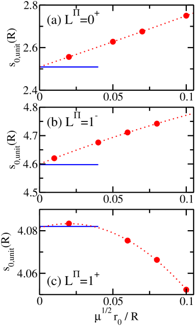
Figure 1: (Color online) Scaled hyperangular eigenvalue $s_{0,{\rm{unit}}}(R)$ for the $(2,2)$ system with $\kappa=1$ at unitarity. Circles show the scaled hyperangular eigenvalue $s_{0,{\rm{unit}}}(R)$ as a function of $\sqrt{\mu}r_{0}/R$ for (a) $L^{\Pi}=0^{+}$ symmetry, (b) $L^{\Pi}=1^{-}$ symmetry, and (c) $L^{\Pi}=1^{+}$ symmetry. The dotted lines show three-parameter fits (using a second-order polynomial). The solid horizontal line in panel (a) shows the result from Ref. vonstecherPRA for $s_{0,{\rm{unit}}}^{\rm{ZR}}$ while the solid horizontal lines in panels (b) and (c) show the results from Ref. debraj for $s_{0,{\rm{unit}}}^{\rm{ZR}}$ (see the text for details). The agreement between our results and those from the literature is very good.

The basis set extrapolation error is smaller than the symbol size. Dotted lines show a fit to the data using the fitting function $s_{0,{\rm{unit}}}^{\rm{ZR}}+c_{1}x+c_{2}x^{2}$, where $x=\sqrt{\mu}r_{0}/R$. The coefficient $s_{0,\rm{unit}}^{\rm{ZR}}$ is found to be $2.510(1)$, $4.600(3)$, and $4.081(3)$ for $L^{\Pi}=0^{+}$, $1^{-}$ and $1^{+}$, respectively. For the $(2,2)$ system with $0^{+}$ symmetry, our results compare well with the value $2.5092$ obtained by von Stecher and Greene vonstecherPRA using the same approach as that employed here. For the $(2,2)$ systems with $1^{-}$ and $1^{+}$ symmetry, the $s_{0,{\rm{unit}}}^{\rm{ZR}}$ value has, to the best of our knowledge, not been calculated within the hyperspherical coordinate approach. However, using scale invariance arguments werner , $s_{0,{\rm{unit}}}^{\rm{ZR}}$ can be extracted from the energy spectrum of the harmonically trapped $(2,2)$ system. The $s_{0,\rm{unit}}^{\rm{ZR}}$ values for the zero-range system at unitarity, obtained by analyzing the energy spectrum of the trapped system, are $s_{0,\rm{unit}}^{\rm{ZR}}=4.5978$ for $L^{\Pi}=1^{-}$ symmetry and $s_{0,\rm{unit}}^{\rm{ZR}}=4.0820$ for $L^{\Pi}=1^{+}$ symmetry debraj . Our values reported above are in very good agreement with these literature values, indicating that the HECG approach is capable of reliably describing strongly-correlated few-body systems with finite angular momentum and positive and negative parity.

To illustrate the convergence of the HECG approach with the number of basis functions, we consider the $(3,1)$ system with $1^{+}$ symmetry ($\kappa=1$ and $1/a_{s}=0$). Solid and dashed lines in Fig. 2 show the scaled hyperangular eigenvalue $s_{0,{\rm{unit}}}(R)$ as a function of the number of basis functions $N_{b}$ for $\sqrt{\mu}r_{0}/R=0.02$ and $\sqrt{\mu}r_{0}/R=0.005$, respectively. For these calculations, we considered $N_{\rm{T}}=4800$ and $6000$ trial functions, respectively, for each new basis function selected.

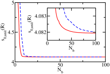
Figure 2: (Color online) Convergence of the scaled hyperangular eigenvalue with increasing number of basis functions $N_{b}$. Solid and dashed lines show the scaled hyperangular eigenvalue $s_{0,{\rm{unit}}}(R)$ as a function of $N_{b}$ for the $(3,1)$ system with $1^{+}$ symmetry and $\kappa=1$ at unitarity for $\sqrt{\mu}r_{0}/R=0.02$ and $\sqrt{\mu}r_{0}/R=0.005$, respectively. The inset shows a blowup.

Figure 2 shows that the description of the system becomes more challenging as the separation of length scales increases, i.e., as the ratio $\sqrt{\mu}r_{0}/R$ decreases. Moreover, it can be seen that $s_{0,{\rm{unit}}}(R)$ shows a few “shoulders”, suggesting that there is room to improve upon the selection of the basis functions. Possible improvements may include gradient optimization techniques, which have been successfully employed in electronic structure calculations gradientoptimization , or a refined trial and error procedure. Nevertheless, the HECG approach in its present implementation yields good convergence for basis sets consisting of around 100 basis functions for the systems under study. The $s_{0,{\rm{unit}}}(R)$ for the largest basis set considered are $4.08194$ and $4.0820$ for $\sqrt{\mu}r_{0}/R=0.02$ and $\sqrt{\mu}r_{0}/R=0.005$, respectively. The corresponding basis set errors are estimated to be smaller than $0.00002$ and $0.0002$, respectively. The dependence of $s_{0,{\rm{unit}}}(R)$ on $r_{0}$ is relatively weak for the $(3,1)$ system with $1^{+}$ symmetry and we find the extrapolated value $s_{0,{\rm{unit}}}^{\rm{ZR}}=4.0820(3)$. This result agrees well with the value of $s_{0,{\rm{unit}}}^{\rm{ZR}}=4.0819$ extracted from the trap energies debraj .

Circles in Fig. 3 shows the scaled hyperangular eigenvalue $s_{0,{\rm{unit}}}(R)$ for the $(3,1)$ system with $\sqrt{\mu}r_{0}/R=0.005$ and $1^{+}$ symmetry ($\kappa=1$ and $1/a_{s}=0$) as a function of the order $N_{\rm{order}}$ used to perform the numerical integration over the hyperangle $\gamma_{2}$. As discussed above, the numerical integral is divided dynamically into three sectors, yielding a total of $3N_{\rm{order}}$ integration points. For the calculations shown in Fig. 3, we used a basis set with $N_{b}=95$. Figure 3 shows that the scaled hyperangular eigenvalue $s_{0,{\rm{unit}}}(R)$ is, for the system considered, accurate to better than 0.1% for $N_{\rm{order}}\gtrsim 60$.

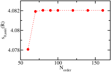
Figure 3: (Color online) Convergence of the scaled hyperangular eigenvalue with increasing number of grid points. The circles show the scaled hyperangular eigenvalue $s_{0,{\rm{unit}}}(R)$, calculated for a basis set consisting of $N_{b}=95$ basis functions, as a function of the order $N_{\rm{order}}$ per sector used to perform the numerical integration over the angle $\gamma_{2}$; as discussed in the text, the numerical integration is divided into three sectors. For $N_{\rm{order}}=50$ (not shown), the numerical integration breaks down (it yields a value that deviates by 10% from the exact value). The calculations are performed for the $(3,1)$ system with $1^{+}$ symmetry, $1/a_{s}=0$, $\kappa=1$ and $\sqrt{\mu}r_{0}/R=0.005$. The dotted line is shown as a guide to the eye.

It is important to note, though, that while $N_{\rm{order}}=60$ yields quite accurate results, $N_{\rm{order}}=50$ yields completely unreliable results for the parameter combination and basis set considered. In practice, we perform the optimization of the basis set for fixed $N_{\rm{order}}$. At the end of the construction of the basis set, we increase $N_{\rm{order}}$ to ensure that the results are independent of the integration scheme employed. In general, the smaller the ratio $\sqrt{\mu}r_{0}/R$, the larger $N_{\rm{order}}$ (assuming the same $L$, $\Pi$, $a_{s}$ and $\kappa$).

As pointed out in Sec. IV, the expressions for the matrix elements presented in the appendices apply to any number of particles. To explicitly confirm this, we performed calculations for the non-interacting five-body systems with $0^{+}$, $1^{-}$ and $1^{+}$ symmetry and found hyperangular eigenvalues consistent with what is expected. Since the matrix elements for the two-body interactions are of the same form as those for the overlaps, treatment of the non-interacting systems suffices for testing the analytical expressions presented in this paper. The computational demands will, of course, increase as the interactions are turned on. Assessing the performance of the outlined formalism for strongly-correlated five-body systems is beyond the scope of this paper.

VI $(3,1)$ system with $1^{+}$ symmetry

This section considers the $(3,1)$ system with $1^{+}$ symmetry at unitarity for various mass ratios. The $s_{0,{\rm{unit}}}^{\rm{ZR}}$ value for these systems has been determined previously blume1 ; blume2 by investigating the $(3,1)$ system under spherically symmetric harmonic confinement using the stochastic variational approach combined with geminal type basis functions, which are neither characterized by good angular momentum and corresponding projection quantum numbers nor good parity. As a result, the earlier calculations were restricted to comparatively large $r_{0}/a_{\rm{ho}}$ values, where $a_{\rm{ho}}$ denotes the harmonic oscillator length of the external confinement. The present work determines $s_{0,{\rm{unit}}}^{\rm{ZR}}$ for various mass ratios $\kappa$ by employing the HECG approach. For comparative purposes, we repeat the trap calculations using the standard ECG approach; however, instead of using geminal type basis functions we employ basis functions which are characterized by good $L$, $M_{L}$ and $\Pi$ quantum numbers, thereby allowing us to reduce the basis set extrapolation error and to treat systems with smaller $r_{0}/a_{\rm{ho}}$ than considered earlier.

Symbols in Fig. 4 show $s_{0,{\rm{unit}}}(R)$ [see Eq. (62)], obtained by the HECG approach, as a function of $\sqrt{\mu}r_{0}/R$ for $\kappa=1,4,8,9.5$ and $10$.

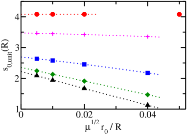
Figure 4: (Color online) $s_{0,{\rm{unit}}}(R)$ as a function of $\sqrt{\mu}r_{0}/R$ for the $(3,1)$ system with $1^{+}$ symmetry at unitarity for $\kappa=1$ (circles), $\kappa=4$ (pluses), $\kappa=8$ (squares), $\kappa=9.5$ (diamonds), and $\kappa=10$ (triangles). Dotted lines show three-parameter fits to the data.

Dotted lines show three-parameter fits. The resulting $s_{0,{\rm{unit}}}^{\rm{ZR}}$ values are summarized in column 2 of Table 1.

Table 1: The first column shows the mass ratio $\kappa$. Columns 2 and 3 show the $s_{0,{\rm{unit}}}^{\rm{ZR}}$ values for the $(3,1)$ system with $1^{+}$ symmetry at unitarity obtained by the HECG approach and from the extrapolated zero-range energies of the trapped system (see the text for details). For comparison, column 4 shows the results from Ref. blume2 . The $\kappa=1$ entry in the third column is taken from Ref. debraj .

$\kappa$	$s_{0,{\rm{unit}}}^{\rm{ZR}}$	$s_{0,{\rm{unit}}}^{\rm{ZR}}$	$s_{0,{\rm{unit}}}^{\rm{ZR}}$
	(HECG)	(trap, this work)	(trap, Ref. blume2 )
$1/10$		4.4256(1)
$1/5$		4.3663(1)
$2/5$		4.2735(1)
$3/5$		4.2000(1)
$4/5$		4.1374(2)
$1$	4.0820(3)	4.0819(1)	4.08
$2$		3.8532(5)	3.86
$3$		3.657(1)
$4$	3.474(4)	3.472(2)	3.51
$8$	2.69(3)	2.68(1)	2.79
$9$		2.41(2)
$19/2$	2.35(6)
$10$	2.22(10)

The errorbars are primarily due to the extrapolation to the $\sqrt{\mu}r_{0}/R\rightarrow 0$ limit and only secondarily due to the basis set extrapolation error of the $s_{0,\rm{unit}}(R)$ for each $R$. Figure 4 suggests that the leading order correction to $s_{0,{\rm{unit}}}^{\rm{ZR}}$ is proportional to $1/R$ for the $\kappa$ values considered ($\kappa>1$). This is in agreement with what has been found analytically for the $(2,1)$ system with $1^{-}$ symmetry kart07 . Figure 4 also shows that the range dependence of $s_{0,{\rm{unit}}}(R)$ increases with increasing $\kappa$. For larger $\kappa$, the range dependence appears to be more complicated and the determination of the corresponding $s_{0,{\rm{unit}}}(R)$ values is beyond the scope of this paper.

Circles in Fig. 5 show the $s_{0,{\rm{unit}}}^{\rm{ZR}}$ values obtained from the HECG approach as a function of $\kappa$.

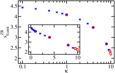
Figure 5: (Color online) $s_{0,{\rm{unit}}}^{\rm{ZR}}$ as a function of $\kappa$ for the $(3,1)$ system with $1^{+}$ symmetry at unitarity. The circles show the $s_{0,{\rm{unit}}}^{\rm{ZR}}$ values determined using the HECG approach while the crosses show the $s_{0,{\rm{unit}}}^{\rm{ZR}}$ values determined by extrapolating the trap energies obtained by the standard ECG approach to the zero-range limit. The errorbars increase with increasing $\kappa$. The agreement between the $s_{0,{\rm{unit}}}^{\rm{ZR}}$ values determined by the two different approaches is very good. The main panel and inset show the same data on different scales; the main panel and inset use respectively logarithmic and linear scales for $\kappa$.

For comparison, crosses show the $s_{0,{\rm{unit}}}^{\rm{ZR}}$ values obtained by extrapolating the finite-range energies of the trapped system to the $r_{0}/a_{\rm{ho}}\rightarrow 0$ limit. These $s_{0,{\rm{unit}}}^{\rm{ZR}}$ values are reported in column 3 of Table 1 and are calculated following the procedure discussed in Ref. debraj for equal masses. The agreement between the two sets of calculations is very good. Column 4 of Table 1 shows the $s_{0,{\rm{unit}}}^{\rm{ZR}}$ values obtained earlier blume2 ; these earlier calculations were restricted to larger $r_{0}/a_{\rm{ho}}$ and are less accurate than the values calculated in this work.

Following the discussion of Refs. petrov ; werner ; blume1 ; blume2 ; nishida , the $s_{0,{\rm{unit}}}^{\rm{ZR}}$ value indicates whether the system behaves universal or not. For two-component Fermi gases with zero-range $s$-wave interactions, e.g., the $s_{0,{\rm{unit}}}^{\rm{ZR}}$ value is larger than 1 and, correspondingly, the system properties are fully determined by $a_{s}$. If $s_{0,{\rm{unit}}}^{\rm{ZR}}<1$, the solution to the hyperradial Schrödinger equation, which is a second order differential equation, can—at least in principle—contain contributions of the “regular” and “irregular” solutions. If the irregular solution contributes, the system is said to behave non-universal since its properties depend not only on the $s$-wave scattering length but additionally on a second parameter. Applying these arguments to the $(3,1)$ system with $1^{+}$ symmetry and using that $s_{0,{\rm{unit}}}^{\rm{ZR}}>1$ for the mass ratios considered, the present study supports the finding that the four-body bound states found in Ref. blum12 for $\kappa\gtrsim 9.5$ and positive $s$-wave scattering length are universal.

VII Conclusions

This paper extended the HECG approach, which had previously been formulated for and applied to three- and four-particle systems with $L^{\Pi}=0^{+}$ symmetry vonstecherPRA ; vonstecherThesis ; ritt11 , to states with $1^{-}$ and $1^{+}$ symmetry. The developed framework is applicable to systems with any $n$; realistically, though, applications in the not too distant future will likely be limited to systems with up to five particles. This paper emphasized a unified formulation for solving the hyperangular Schrödinger equation. In particular, many of the resulting equations apply to any particle number and $L^{\Pi}$ symmetry, suggesting a numerical implementation in which most subroutines can be used for any particle number $n$ and any $L^{\Pi}$ symmetry; only a few subroutines specific to the values of $n$, $L$ and $\Pi$ are needed.

As a first application, we considered the $(2,2)$ and $(3,1)$ systems at unitarity. In particular, we solved the hyperangular Schrödinger equation for the energetically lowest-lying eigenvalue in the small $\sqrt{\mu}r_{0}/R$ regime and extracted the corresponding $s_{0,{\rm{unit}}}^{\rm{ZR}}$ values. Our results are in very good agreement with results from the literature and with results determined by an alternative approach. The $s_{0,{\rm{unit}}}^{\rm{ZR}}$ values for the $(3,1)$ system at unitarity with $1^{+}$ symmetry consisting of three heavy identical fermions and one light impurity particle are relevant to the $(3,1)$ system with positive $a_{s}$. In particular, the results obtained in this paper lend strong support that the bound states of the $(3,1)$ system with positive $s$-wave scattering length found in Ref. blum12 are universal, i.e., fully determined by $a_{s}$. While we were able to reliably describe four-body systems for which the hyperradius $R$ is 200 times larger than the scaled range $\sqrt{\mu}r_{0}$ of the two-body potential, pushing this ratio to much larger values may be challenging.

In the future, it will be interesting to combine, as done in Refs. vonstecherPRA ; vonstecherThesis ; ritt11 , the developed framework with a standard R-matrix approach and to describe the scattering properties of four-particle systems with finite angular momentum. The generalization of the developed formalism to states with other $L^{\Pi}$ symmetries, which amounts to determining the corresponding $d$-, $b$-, $p$- and $q$-coefficients, is tedious but straightforward. Other possible extensions include the generalization of the approach to cold atom systems in a wave guide geometry.

Appendix A Definition of (symmetry-dependent) auxiliary quantities

We first introduce a number of auxiliary quantities and then define quantities specific to the basis functions with $L^{\Pi}=0^{+},1^{-}$ and $1^{+}$ symmetry.

The matrix $\underline{S}$ is defined as

$$\underline{S}=\underline{A}_{B}\underline{A}_{B}^{\prime}+\underline{A}_{B}^{\prime}\underline{A}_{B},$$ (63)

where

$$\underline{A}_{B}=(\underline{U}_{B})^{T}\underline{A}\underline{U}_{B}$$ (64)

and

$$\underline{A}_{B}^{\prime}=(\underline{U}_{B})^{T}\underline{A}^{\prime}\underline{U}_{B}.$$ (65)

Similarly, we define

$$\underline{B}_{B}=\underline{A}_{B}+\underline{A}^{\prime}_{B}.$$ (66)

We define the vectors $\vec{u}_{j,B}$ and $\vec{u}_{j,B}^{\prime}$ ($j=1$ and 2),

$$\vec{u}_{j,B}=\left(\underline{U}_{B}\right)^{T}\vec{u}_{j}$$ (67)

and

$$\vec{u}_{j,B}^{\prime}=\left(\underline{U}_{B}\right)^{T}\vec{u}_{j}^{\prime}.$$ (68)

Lastly, we define

$$a(j,k)=u_{1,B}(j)u_{1,B}^{\prime}(k),$$ (69)

$$\bar{a}(j,k)=u_{2,B}(j)u_{2,B}^{\prime}(k),$$ (70)

$$g(j,k,l)=a(j,j)\bar{a}(l,k)+a(l,k)\bar{a}(j,j)-$$

$$a(l,j)\bar{a}(j,k)-a(j,k)\bar{a}(l,j),$$ (71)

$$\bar{g}(j,k,l)=g(j,l,k),$$ (72)

$$h(j,k,l)=g(l,j,k)+\bar{g}(l,j,k),$$ (73)

$$F(j,k,l,m)=a(j,k)\bar{a}(l,m)+a(k,j)\bar{a}(l,m)+$$

$$a(j,k)\bar{a}(m,l)+a(k,j)\bar{a}(m,l),$$ (74)

$$G(j,k,l,m)=a(j,l)\bar{a}(m,k)+a(j,m)\bar{a}(l,k)+$$

$$a(k,l)\bar{a}(m,j)+a(k,m)\bar{a}(l,j),$$ (75)

and

$$f(j,k,l,m)=F(j,k,l,m)+F(l,m,j,k)-$$

$$G(j,k,l,m)-G(l,m,j,k).$$ (76)

Sections A.1-A.3 give explicit expressions for the $d$-, $p$-, $q$- and $b$-coefficients for the basis functions with $0^{+}$, $1^{-}$ and $1^{+}$ symmetry, respectively. In what follows, the elements of the vector $\vec{u}_{j,B}$ are denoted by ${u}_{j,B}(k)$, $k=1,\cdots,n-1$; the same notation is adopted for the elements of other vectors. The elements of the matrix $\underline{S}$ are denoted by $\underline{S}(k,l)$ with $k$ and $l=1,\cdots,n-1$; the same notation is adopted for the elements of other matrices.

A.1 $0^{+}$ symmetry

The only non-zero $d$-coefficient is $d^{(0)}$,

$$d^{(0)}=1.$$ (77)

The only non-zero $p$-coefficient is $p_{j}^{(2)}$,

$$p_{j}^{(2)}=\underline{A}_{B}(j,j)R^{-1}.$$ (78)

The non-zero $q$-coefficients are $q_{j}^{(2)}$, $q_{j}^{(4)}$ and $q_{j,k}^{(22)}$,

$$q_{j}^{(2)}=R^{-1}p_{j}^{(2)},$$ (79)

$$q_{j}^{(4)}=-\underline{A}_{B}^{2}(j,j)R^{-2},$$ (80)

and

$$q_{j,k}^{(22)}=-\left[2\underline{A}_{B}(j,j)\underline{A}_{B}(k,k)+\frac{4}{3}\underline{A}_{B}^{2}(j,k)\right]R^{-2}.$$ (81)

Here, $\underline{A}_{B}^{2}(j,k)$ denotes the square of the matrix element $\underline{A}_{B}(j,k)$.

The non-zero $b$-coefficients are $b^{(0)}$, $b_{j}^{(2)}$, $b_{j}^{(4)}$ and $b^{(22)}_{j,k}$,

$$b^{(0)}=-3\mbox{Tr}(\underline{B}_{B}),$$ (82)

$$b_{j}^{(2)}=\beta_{j}^{2}-\underline{S}(j,j)+(3n-3)\beta_{j}R^{-2},$$ (83)

$$b_{j}^{(4)}=\left[-\beta_{j}^{2}+2\underline{A}_{B}(j,j)\underline{A}_{B}^{\prime}(j,j)\right]R^{-2},$$ (84)

and

$$b_{j,k}^{(22)}=-2\beta_{j}\beta_{k}R^{-2}+2\underline{A}_{B}(j,j)\underline{A}_{B}^{\prime}(k,k)R^{-2}+$$

$$2\underline{A}_{B}(k,k)\underline{A}_{B}^{\prime}(j,j)R^{-2}+\frac{8}{3}\underline{A}_{B}(j,k)\underline{A}_{B}^{\prime}(j,k)R^{-2}.$$ (85)

A.2 $1^{-}$ symmetry

The only non-zero $d$-coefficient is $d^{(2)}_{j}$,

$$d^{(2)}_{j}=a(j,j).$$ (86)

The non-zero $p$-coefficients are $p_{j}^{(2)}$, $p_{j}^{(4)}$ and $p_{j,k}^{(22)}$,

$$p_{j}^{(2)}=-a(j,j)R^{-1},$$ (87)

$$p_{j}^{(4)}=\underline{A}_{B}(j,j)a(j,j)R^{-1},$$ (88)

and

$$p_{j,k}^{(22)}=\underline{A}_{B}(j,j)a(k,k)R^{-1}+$$

$$\underline{A}_{B}(k,k)a(j,j)R^{-1}+$$

$$\frac{2}{3}\underline{A}_{B}(j,k)\left[a(j,k)+a(k,j)\right]R^{-1}.$$ (89)

The non-zero $q$-coefficients are $q_{j}^{(4)}$, $q_{j,k}^{(22)}$, $q_{j}^{(6)}$, $q_{j,k}^{(24)}$ and $q_{j,k,l}^{(222)}$,

$$q_{j}^{(4)}=3R^{-1}p_{j}^{(4)},$$ (90)

$$q_{j,k}^{(22)}=3R^{-1}p_{j,k}^{(22)},$$ (91)

$$q_{j}^{(6)}=-\underline{A}_{B}^{2}(j,j)a(j,j)R^{-2},$$ (92)

$$q_{j,k}^{(24)}=-\underline{A}_{B}^{2}(k,k)a(j,j)R^{-2}-$$

$$2\underline{A}_{B}(j,j)\underline{A}_{B}(k,k)a(k,k)R^{-2}-$$

$$\frac{4}{3}\underline{A}_{B}^{2}(j,k)a(k,k)R^{-2}-$$

$$\frac{4}{3}\underline{A}_{B}(k,k)\underline{A}_{B}(j,k)\left[a(j,k)+a(k,j)\right]R^{-2}$$ (93)

and

$$q_{j,k,l}^{(222)}=$$

$$\left[-2\underline{A}_{B}(j,j)\underline{A}_{B}(k,k)a(l,l)-\frac{4}{3}\underline{A}_{B}^{2}(j,k)a(l,l)\right]R^{-2}+$$

$$\left[-\frac{4}{3}\underline{A}_{B}(j,k)\underline{A}_{B}(l,l)-\frac{8}{9}\underline{A}_{B}(j,l)\underline{A}_{B}(k,l)\right]\times$$

$$\left[a(j,k)+a(k,j)\right]R^{-2}.$$ (94)

The non-zero $b$-coefficients are $b_{j}^{(2)}$, $b_{j}^{(4)}$, $b_{j}^{(6)}$, $b_{j,k}^{(22)}$, $b_{j,k}^{(24)}$ and $b_{j,k,l}^{(222)}$,

$$b^{(2)}_{j}=-2(3n-4)a(j,j)R^{-2}-$$

$$2\sum_{k=1}^{n-1}\left[\underline{A}_{B}(j,k)a(k,j)+\underline{A}^{\prime}_{B}(j,k)a(j,k)\right]-$$

$$3\mbox{Tr}(\underline{B}_{B})a(j,j),$$ (95)

$$b^{(4)}_{j}=\left[\beta_{j}^{2}-\underline{S}(j,j)+(3n-1)\beta_{j}R^{-2}\right]a(j,j),$$ (96)

$$b^{(6)}_{j}=\left[-\beta_{j}^{2}+2\underline{A}_{B}(j,j)\underline{A}_{B}^{\prime}(j,j)\right]a(j,j)R^{-2},$$ (97)

$$b^{(22)}_{j,k}= \left[\beta_{j}^{2}-\underline{S}(j,j)+(3n-1)\beta_{j}R^{-2}\right]a(k,k)+$$ (98)

$$\left[\beta_{k}^{2}-\underline{S}(k,k)+(3n-1)\beta_{k}R^{-2}\right]a(j,j)-$$

$$\frac{1}{3}\left[\underline{S}(j,k)+\underline{S}(k,j)\right]\left[a(j,k)+a(k,j)\right],$$

$$b_{j,k}^{(24)}= \left[-\beta_{k}^{2}+2\underline{A}_{B}(k,k)\underline{A}_{B}^{\prime}(k,k)\right]a(j,j)R^{-2}+$$ (99)

$$\big{[}-2\beta_{j}\beta_{k}+2\underline{A}_{B}(j,j)\underline{A}^{\prime}_{B}(k,k)+$$

$$2\underline{A}_{B}(k,k)\underline{A}^{\prime}_{B}(j,j)+\frac{8}{3}\underline{A}_{B}(j,k)\underline{A}_{B}^{\prime}(j,k)\big{]}\times$$

$$a(k,k)R^{-2}+$$

$$\frac{4}{3}\left[\underline{A}_{B}(j,k)\underline{A}_{B}^{\prime}(k,k)+\underline{A}_{B}(k,k)\underline{A}_{B}^{\prime}(j,k)\right]\times$$

$$\left[a(j,k)+a(k,j)\right]R^{-2}$$

and

$$b_{j,k,l}^{(222)}= \big{[}-2\beta_{j}\beta_{k}+2\underline{A}_{B}(j,j)\underline{A}_{B}^{\prime}(k,k)+$$ (100)

$$2\underline{A}_{B}(k,k)\underline{A}_{B}^{\prime}(j,j)+\frac{8}{3}\underline{A}_{B}(j,k)\underline{A}^{\prime}(j,k)\big{]}\times$$

$$a(l,l)R^{-2}+$$

$$\frac{4}{3}\left[\underline{A}_{B}(j,k)\underline{A}_{B}^{\prime}(l,l)+\underline{A}_{B}(l,l)\underline{A}_{B}^{\prime}(j,k)\right]\times$$

$$\left[a(j,k)+a(k,j)\right]R^{-2}+$$

$$\frac{8}{9}\left[\underline{A}_{B}(j,l)\underline{A}_{B}^{\prime}(k,l)+\underline{A}_{B}(k,l)\underline{A}_{B}^{\prime}(j,l)\right]\times$$

$$\left[a(j,k)+a(k,j)\right]R^{-2}.$$

A.3 $1^{+}$ symmetry

The only non-zero $d$-coefficient is $d_{j,k}^{(22)}$,

$$d_{j,k}^{(22)}=a(j,j)\bar{a}(k,k)+a(k,k)\bar{a}(j,j)-$$

$$a(j,k)\bar{a}(k,j)-a(k,j)\bar{a}(j,k).$$ (101)

The non-zero $p$-coefficients are $p_{j,k}^{(22)}$, $p_{j,k}^{(24)}$ and $p_{j,k,l}^{(222)}$,

$$p_{j,k}^{(22)}=-2R^{-1}d_{j,k}^{(22)},$$ (102)

$$p_{j,k}^{(24)}=R^{-1}d_{j,k}^{(22)}\underline{A}_{B}(k,k),$$ (103)

and

$$p_{j,k,l}^{(222)}=R^{-1}d_{j,k}^{(22)}\underline{A}_{B}(l,l)+$$

$$\frac{2}{3}R^{-1}\underline{A}_{B}(j,k)h(j,k,l).$$ (104)

The non-zero $q$-coefficients are $q_{j,k}^{(22)}$, $q_{j,k}^{(24)}$, $q_{j,k,l}^{(222)}$, $q_{j,k}^{(26)}$, $q_{j,k}^{(44)}$, $q_{j,k,l}^{(224)}$ and $q_{j,k,l,m}^{(2222)}$,

$$q_{j,k}^{(22)}=R^{-1}p_{j,k}^{(22)},$$ (105)

$$q_{j,k}^{(24)}=5R^{-1}p_{j,k}^{(24)},$$ (106)

$$q_{j,k,l}^{(222)}=5R^{-1}p_{j,k,l}^{(222)},$$ (107)

$$q_{j,k}^{(26)}=-d_{j,k}^{(22)}\underline{A}_{B}^{2}(k,k)R^{-2},$$ (108)

$$q_{j,k}^{(44)}=-2d_{j,k}^{(22)}\underline{A}_{B}(j,j)\underline{A}_{B}(k,k)R^{-2}-$$

$$\frac{4}{5}d_{j,k}^{(22)}\underline{A}_{B}^{2}(j,k)R^{-2},$$ (109)

$$q_{j,k,l}^{(224)}= -\left[\underline{A}_{B}(j,j)\underline{A}_{B}(l,l)+\frac{2}{3}\underline{A}_{B}^{2}(j,l)\right]2R^{-2}d_{k,l}^{(22)}-$$ (110)

$$\left[\underline{A}_{B}(k,k)\underline{A}_{B}(l,l)+\frac{2}{3}\underline{A}_{B}^{2}(k,l)\right]2R^{-2}d_{j,l}^{(22)}-$$

$$\underline{A}_{B}^{2}(l,l)R^{-2}d_{j,k}^{(22)}-$$

$$\frac{4}{3}\big{[}\underline{A}_{B}(j,k)\underline{A}_{B}(l,l)h(j,k,l)+$$

$$\underline{A}_{B}(j,l)\underline{A}_{B}(l,l)h(j,l,k)+$$

$$\underline{A}_{B}(k,l)\underline{A}_{B}(l,l)h(k,l,j)\big{]}R^{-2},$$

and

$$q_{j,k,l,m}^{(2222)}=$$

$$-\left[2\underline{A}_{B}(l,l)\underline{A}_{B}(m,m)+\frac{4}{3}\underline{A}_{B}^{2}(l,m)\right]R^{-2}d_{jk}^{(22)}-$$

$$\left[2\underline{A}_{B}(j,j)\underline{A}_{B}(k,k)+\frac{4}{3}\underline{A}_{B}^{2}(j,k)\right]R^{-2}d_{lm}^{(22)}-$$

$$\frac{4}{3}\big{[}\underline{A}_{B}(j,k)\underline{A}_{B}(m,m)h(j,k,l)+$$

$$\underline{A}_{B}(j,k)\underline{A}_{B}(l,l)h(j,k,m)\big{]}R^{-2}-$$

$$\frac{4}{3}\big{[}\underline{A}_{B}(l,m)\underline{A}_{B}(k,k)h(l,m,j)+$$

$$\underline{A}_{B}(l,m)\underline{A}_{B}(j,j)h(l,m,k)\big{]}R^{-2}-$$

$$\frac{8}{9}\big{[}\underline{A}_{B}(l,k)\underline{A}_{B}(k,m)h(l,m,j)+$$

$$\underline{A}_{B}(l,j)\underline{A}_{B}(j,m)h(l,m,k)\big{]}R^{-2}-$$

$$\frac{8}{9}\big{[}\underline{A}_{B}(j,m)\underline{A}_{B}(m,k)h(j,k,l)+$$

$$\underline{A}_{B}(j,l)\underline{A}_{B}(l,k)h(j,k,m)\big{]}R^{-2}-$$

$$\frac{8}{9}\left[\underline{A}_{B}(j,k)\underline{A}_{B}(l,m)\right]f(j,k,l,m)R^{-2}.$$ (111)

The non-zero $b$-coefficients are

$$b_{j,k}^{(22)} = -5\mbox{Tr}(\underline{B}_{B})d_{j,k}^{(22)}-4(3n-3)R^{-2}d_{j,k}^{(22)}-$$ (112)

$$2\sum_{l\neq j,k}^{n-1}\big{[}\underline{A}_{B}(j,l)g(k,j,l)+\underline{A}_{B}^{\prime}(j,l)\bar{g}(k,j,l)+$$

$$\underline{A}_{B}(k,l)g(j,k,l)+\underline{A}_{B}^{\prime}(k,l)\bar{g}(j,k,l)-$$

$$\beta_{l}d_{jk}^{(22)}\big{]},$$

$$b_{j,k}^{(24)}=\left[\beta_{k}^{2}-\underline{S}(k,k)\right]d_{j,k}^{(22)}+\beta_{k}(3n+1)R^{-2}d_{j,k}^{(22)},$$ (113)

$$b_{j,k,l}^{(222)}=\left[\beta_{l}^{2}-\underline{S}(l,l)\right]d_{j,k}^{(22)}-$$

$$\frac{2}{3}h(j,k,l)\underline{S}(j,k)+\beta_{l}(3n+1)R^{-2}d_{j,k}^{(22)},$$ (114)

$$b_{j,k}^{(44)}=\big{[}-\beta_{j}\beta_{k}+\underline{A}_{B}(j,j)\underline{A}_{B}^{\prime}(k,k)+$$

$$\underline{A}_{B}(k,k)\underline{A}_{B}^{\prime}(j,j)+\frac{4}{5}\underline{A}_{B}(j,k)\underline{A}_{B}^{\prime}(j,k)\big{]}2R^{-2}d_{j,k}^{(22)},$$ (115)

$$b_{j,k}^{(26)}=\left[-\beta_{k}^{2}+2\underline{A}_{B}(k,k)\underline{A}^{\prime}_{B}(k,k)\right]R^{-2}d_{j,k}^{(22)},$$ (116)

$$b_{j,k,l}^{(224)}=\big{[}-\beta_{j}\beta_{l}+\underline{A}_{B}(j,j)\underline{A}_{B}^{\prime}(l,l)+\underline{A}_{B}(l,l)\underline{A}_{B}^{\prime}(j,j)+$$

$$\frac{4}{3}\underline{A}_{B}(j,l)\underline{A}_{B}^{\prime}(j,l)\big{]}2R^{-2}d_{k,l}^{(22)}+$$

$$\big{[}-\beta_{k}\beta_{l}+\underline{A}_{B}(k,k)\underline{A}_{B}^{\prime}(l,l)+\underline{A}_{B}(l,l)\underline{A}_{B}^{\prime}(k,k)+$$

$$\frac{4}{3}\underline{A}_{B}(k,l)\underline{A}_{B}^{\prime}(k,l)\big{]}2R^{-2}d_{j,l}^{(22)}+$$

$$\left[-\beta_{l}^{2}+2\underline{A}_{B}(l,l)\underline{A}_{B}^{\prime}(l,l)\right]R^{-2}d_{j,k}^{(22)}-$$

$$\frac{4}{3}\left[\underline{A}_{B}(j,k)\underline{A}_{B}(l,l)+\underline{A}_{B}^{\prime}(j,k)\underline{A}_{B}^{\prime}(l,l)\right]R^{-2}h(j,k,l)-$$

$$\frac{4}{3}\left[\underline{A}_{B}(j,l)\underline{A}_{B}(l,l)+\underline{A}_{B}^{\prime}(j,l)\underline{A}_{B}^{\prime}(l,l)\right]R^{-2}h(j,l,k)-$$

$$\frac{4}{3}\left[\underline{A}_{B}(k,l)\underline{A}_{B}(l,l)+\underline{A}_{B}^{\prime}(k,l)\underline{A}_{B}^{\prime}(l,l)\right]R^{-2}h(k,l,j),$$ (117)

and

$$b_{j,k,l,m}^{(2222)}=$$

$$-\big{\{}2\underline{A}_{B}(l,l)\underline{A}_{B}(m,m)+2\underline{A}_{B}^{\prime}(l,l)\underline{A}_{B}^{\prime}(m,m)+$$

$$\frac{4}{3}\left[\underline{A}_{B}^{2}(l,m)+\underline{A}_{B}^{\prime 2}(l,m)\right]\big{\}}R^{-2}d_{jk}^{(22)}-$$

$$\big{\{}2\underline{A}_{B}(j,j)\underline{A}_{B}(k,k)+2\underline{A}_{B}^{\prime}(j,j)\underline{A}_{B}^{\prime}(k,k)+$$

$$\frac{4}{3}\left[\underline{A}_{B}^{2}(j,k)+\underline{A}_{B}^{\prime 2}(j,k)\right]\big{\}}R^{-2}d_{lm}^{(22)}-$$

$$\frac{4}{3}\left[\underline{A}_{B}(j,k)\underline{A}_{B}(m,m)+\underline{A}_{B}^{\prime}(j,k)\underline{A}_{B}^{\prime}(m,m)\right]\times$$

$$h(j,k,l)R^{-2}-$$

$$\frac{4}{3}\left[\underline{A}_{B}(j,k)\underline{A}_{B}(l,l)+\underline{A}_{B}^{\prime}(j,k)\underline{A}_{B}^{\prime}(l,l)\right]\times$$

$$h(j,k,m)R^{-2}-$$

$$\frac{4}{3}\left[\underline{A}_{B}(l,m)\underline{A}_{B}(k,k)+\underline{A}_{B}^{\prime}(l,m)\underline{A}_{B}^{\prime}(k,k)\right]\times$$

$$h(l,m,j)R^{-2}-$$

$$\frac{4}{3}\left[\underline{A}_{B}(l,m)\underline{A}_{B}(j,j)+\underline{A}_{B}^{\prime}(l,m)\underline{A}_{B}^{\prime}(j,j)\right]\times$$

$$h(l,m,k)R^{-2}-$$

$$\frac{8}{9}\left[\underline{A}_{B}(l,k)\underline{A}_{B}(k,m)+\underline{A}^{\prime}_{B}(l,k)\underline{A}^{\prime}_{B}(k,m)\right]\times$$

$$h(l,m,j)R^{-2}-$$

$$\frac{8}{9}\left[\underline{A}_{B}(l,j)\underline{A}_{B}(j,m)+\underline{A}^{\prime}_{B}(l,j)\underline{A}^{\prime}_{B}(j,m)\right]\times$$

$$h(l,m,k)R^{-2}-$$

$$\frac{8}{9}\left[\underline{A}_{B}(j,m)\underline{A}_{B}(m,k)+\underline{A}^{\prime}_{B}(j,m)\underline{A}^{\prime}_{B}(m,k)\right]\times$$

$$h(j,k,l)R^{-2}-$$

$$\frac{8}{9}\left[\underline{A}_{B}(j,l)\underline{A}_{B}(l,k)+\underline{A}^{\prime}_{B}(j,l)\underline{A}^{\prime}_{B}(l,k)\right]h(j,k,m)R^{-2}-$$

$$\frac{8}{9}\left[\underline{A}_{B}(j,k)\underline{A}_{B}(l,m)+\underline{A}_{B}^{\prime}(j,k)\underline{A}_{B}^{\prime}(l,m)\right]\times$$

$$f(j,k,l,m)R^{-2}.$$ (118)

Appendix B Sketch of derivation of matrix elements for $n=3$ and $L^{\Pi}=1^{-}$ symmetry

This appendix derives the overlap matrix element for $n=3$ and $L^{\Pi}=1^{-}$. To evaluate the overlap matrix element, we write, using Eq. (37),

$$\psi(\underline{A}^{\prime},\vec{u}_{1}^{\prime},\vec{x})\psi(\underline{A},\vec{u}_{1},\vec{x})=3v_{1,3}^{\prime}v_{1,3}\exp\left(-\frac{\vec{x}^{T}\underline{B}\vec{x}}{2}\right),$$ (119)

where $\underline{B}$ is defined in Eq. (43). Using the transformation $\vec{y}=\underline{U}_{B}^{T}\vec{x}$, we find

$$v_{1,3}^{\prime}v_{1,3}=$$

$$a(1,1)y_{1,3}^{2}+\left[a(1,2)+a(2,1)\right]y_{1,3}y_{2,3}+a(2,2)y_{2,3}^{2},$$ (120)

where $a(i,j)$ is defined in Eq. (69) and where $y_{j,3}$ denotes the $z$-component of the vector $\vec{y}_{j}$. Using $y_{1,3}=y_{1}\cos\vartheta_{1}$ and $y_{2,3}=y_{2}\cos\vartheta_{2}$ in Eqs. (119) and (B), we have

$$\psi^{\prime}\psi=3\big{\{}a(1,1)y_{1}^{2}\cos^{2}\vartheta_{1}+$$

$$\left[a(1,2)+a(2,1)\right]y_{1}y_{2}\cos\vartheta_{1}\cos\vartheta_{2}+a(2,2)y_{2}^{2}\cos^{2}\vartheta_{2}\big{\}}\times$$

$$\exp\left[-\frac{1}{2}\left(\beta_{1}y_{1}^{2}+\beta_{2}y_{2}^{2}\right)\right],$$ (121)

where the $\beta_{j}$ denote, as before, the eigenvalues of the matrix $\underline{B}$. When integrating over $\hat{y}_{1}\hat{y}_{2}$, the cross term averages to zero and we have

$$\int_{0}^{2\pi}\int_{-1}^{1}\int_{0}^{2\pi}\int_{-1}^{1}\left(\psi^{\prime}\psi\right)|_{R}d\cos\vartheta_{1}d\varphi_{1}d\cos\vartheta_{2}d\varphi_{2}=$$

$$(4\pi)^{2}\left[a(1,1)y_{1}^{2}+a(2,2)y_{2}^{2}\right]\times$$

$$\exp\left[-\frac{1}{2}\left(\beta_{1}y_{1}^{2}+\beta_{2}y_{2}^{2}\right)\right].$$ (122)

Comparison of Eq. (B) with Eq. (IV) shows that $d_{j}^{(2)}=a(j,j)$ and that all other $d$-coefficients are zero. This agrees with the expressions given in Appendix A.2.

Next, we consider the integration over $\gamma_{1}$. To this end, we replace $y_{1}$ and $y_{2}$ in Eq. (B) by $R\sin\gamma_{1}$ and $R\cos\gamma_{1}$, respectively. According to the discussion in Sec. IV, $\gamma_{1}$ can take values between $0$ and $\pi/2$. Multiplying both sides of Eq. (B) by $\sin^{2}\gamma_{1}\cos^{2}\gamma_{1}$ [see Eq. (IV)] and integrating over $\gamma_{1}$, we find

$$\int\left(\psi^{\prime}\psi\right)|_{R}d^{5}\vec{\Omega}=(4\pi)^{2}\frac{\pi}{16\zeta}\exp\left[-\frac{1}{4}R^{2}(\beta_{1}+\beta_{2})\right]\times$$

$$\big{\{}\left[a(1,1)+a(2,2)\right]R^{2}I_{1}(\zeta)+$$

$$\left[-a(1,1)+a(2,2)\right]R^{2}I_{2}(\zeta)\big{\}}.$$ (123)

Applying the definitions from Appendix A and C, it can be verified that Eq. (B) agrees with Eq. (IV) [note that Eq. (IV) does not contain a factor of $(4\pi)^{2}$ while Eq. (B) does; the reason is that $f_{o}$ is defined without this prefactor].

The derivation sketched above for the overlap matrix element can be fairly straightforwardly generalized to arbitrary $n$. To calculate the matrix element $\langle\psi|T_{\Omega}|\psi\rangle|_{R}$, we use Eq. (27), i.e., we separately calculate the matrix elements $\langle\psi|T_{\rm{rel}}|\psi\rangle|_{R}$ and $\langle\psi|T_{R}|\psi\rangle|_{R}$. The evaluation of these matrix elements is not fundamentally difficult but somewhat tedious and lengthy.

Appendix C Definitions of $sc$-coefficients, $M_{1}$ and $M_{2}$

The $sc$-coefficients entering into $f_{o}$ are given by

$$sc_{00} = d^{(0)}+\sum_{j=3}^{n-1}\left[d^{(2)}_{j}y_{j}^{2}+d^{(4)}_{j}y_{j}^{4}+d^{(6)}_{j}y_{j}^{6}\right]+$$ (124)

$$\sum_{k>j;j,k\neq 1,2}^{n-1}\left[d^{(22)}_{j,k}y_{j}^{2}y_{k}^{2}+d^{(44)}_{j,k}y_{j}^{4}y_{k}^{4}\right]+$$

$$\sum_{j=3,k=3,k\neq j}^{n-1}\left[d^{(24)}_{j,k}y_{j}^{2}y_{k}^{4}+d^{(26)}_{j,k}y_{j}^{2}y_{k}^{6}\right]+$$

$$\sum_{k>j;l\neq j,k;j,k,l\neq 1,2}^{n-1}\left[d^{(222)}_{j,k,l}y_{j}^{2}y_{k}^{2}y_{l}^{2}+d^{(224)}_{j,k,l}y_{j}^{2}y_{k}^{2}y_{l}^{4}\right]+$$

$$\sum_{k>j;l>j;m>l;j\neq k\neq l\neq m;j,k,l,m\neq 1,2}^{n-1}d_{j,k,l,m}^{(2222)}y_{j}^{2}y_{k}^{2}k_{l}^{2}y_{m}^{2},$$

$$sc_{20} = d^{(2)}_{1}+\sum_{j=3}^{n-1}\left[d_{1,j}^{(22)}y_{j}^{2}+d^{(24)}_{1,j}y_{j}^{4}+d^{(26)}_{1,j}y_{j}^{6}\right]+$$ (125)

$$\sum_{j,k=3;k\neq j}^{n-1}\left[d^{(222)}_{1,j,k}y_{j}^{2}y_{k}^{2}+d^{(224)}_{1,j,k}y_{j}^{2}y_{k}^{4}\right]+$$

$$\sum_{j<k;j,k\neq 1,2}^{n-1}d^{(222)}_{j,k,1}y_{j}^{2}y_{k}^{2}+$$

$$\sum_{l>k;j\neq k\neq l;j,k,l\neq 1,2}^{n-1}d_{1,j,k,l}^{(2222)}y_{j}^{2}y_{k}^{2}k_{l}^{2},$$

$$sc_{02} = d^{(2)}_{2}+\sum_{j=3}^{n-1}\left[d_{2,j}^{(22)}y_{j}^{2}+d^{(24)}_{2,j}y_{j}^{4}+d^{(26)}_{2,j}y_{j}^{6}\right]+$$ (126)

$$\sum_{j,k=3;k\neq j}^{n-1}\left[d^{(222)}_{2,j,k}y_{j}^{2}y_{k}^{2}+d^{(224)}_{2,j,k}y_{j}^{2}y_{k}^{4}\right]+$$

$$\sum_{j<k;j,k\neq 1,2}^{n-1}d^{(222)}_{j,k,2}y_{j}^{2}y_{k}^{2}+$$

$$\sum_{l>k;j\neq k\neq l;j,k,l\neq 1,2}^{n-1}d_{2,j,k,l}^{(2222)}y_{j}^{2}y_{k}^{2}y_{l}^{2},$$

$$sc_{40} = d_{1}^{(4)}+\sum_{j=3}^{n-1}\left[d_{1,j}^{(44)}y_{j}^{4}+d_{j,1}^{(24)}y_{j}^{2}\right]+$$ (127)

$$\sum_{j<k;j,k\neq 1,2}^{n-1}d_{j,k,1}^{(224)}y_{j}^{2}y_{k}^{2},$$

$$sc_{04} = d_{2}^{(4)}+\sum_{j=3}^{n-1}\left[d_{2,j}^{(44)}y_{j}^{4}+d_{j,2}^{(24)}y_{j}^{2}\right]+$$ (128)

$$\sum_{j<k;j,k\neq 1,2}^{n-1}d_{j,k,2}^{(224)}y_{j}^{2}y_{k}^{2},$$

$$sc_{60} = d_{1}^{(6)}+\sum_{j=3}^{n-1}d_{j,1}^{(26)}y_{j}^{2},$$ (129)

$$sc_{06} = d_{2}^{(6)}+\sum_{j=3}^{n-1}d_{j,2}^{(26)}y_{j}^{2},$$ (130)

$$sc_{22} = d_{1,2}^{(22)}+$$ (131)

$$\sum_{j=3}^{n-1}\left\{\left[d_{1,2,j}^{(222)}+d_{1,j,2}^{(222)}+d_{2,j,1}^{(222)}\right]y_{j}^{2}+d_{1,2,j}^{(224)}y_{j}^{4}\right\}+$$

$$\sum_{j<k;j,k\neq 1,2}^{n-1}d_{12jk}^{(2222)}y_{j}^{2}y_{k}^{2}+$$

$$\sum_{j\neq k;j,k\neq 1,2}^{n-1}d_{1j2k}^{(2222)}y_{j}^{2}y_{k}^{2},$$

$$sc_{44} = d_{1,2}^{(44)},$$ (132)

$$sc_{24} = d_{1,2}^{(24)}+\sum_{j=3}^{n-1}d_{1,j,2}^{(224)}y_{j}^{2},$$ (133)

$$sc_{42} = d_{2,1}^{(24)}+\sum_{j=3}^{n-1}d_{2,j,1}^{(224)}y_{j}^{2},$$ (134)

$$sc_{26} = d_{1,2}^{(26)},$$ (135)

and

$$sc_{62} = d_{2,1}^{(26)}.$$ (136)

Equation (124)-(136) also apply to $f_{P}$, $f_{Q}$ and $f_{\Omega}$ if the $d$-coefficients are replaced by the $p$-, $q$- and $b$-coefficients, respectively. The quantities $M_{1}$ and $M_{2}$ are defined through

$$M_{1}=-\frac{1}{4}M_{\rm{aux}}+\big{[}2sc_{00}+(sc_{20}+sc_{02})HR^{2}+$$

$$(sc_{40}+sc_{04})(HR^{2})^{2}+(sc_{60}+sc_{06})(HR^{2})^{3}\big{]}\zeta$$ (137)

and

$$M_{2}=\zeta^{-1}M_{\rm{aux}}+\frac{3}{4}\big{[}-2sc_{40}-2sc_{04}+2sc_{22}+$$

$$(-3sc_{60}-3sc_{06}+sc_{24}+sc_{42})HR^{2}+$$

$$(sc_{26}+sc_{62})(HR^{2})^{2}\big{]}(HR^{2})^{2}+$$

$$\big{[}-sc_{20}+sc_{02}+(-sc_{40}+sc_{04})HR^{2}+$$

$$(-sc_{60}+sc_{06})(HR^{2})^{2}\big{]}HR^{2}\zeta,$$ (138)

where

$$M_{\rm{aux}}=-\frac{15}{2}(-sc_{26}+sc_{44}-sc_{62})(HR^{2})^{4}\zeta^{-1}+$$

$$3\big{[}-sc_{60}+sc_{06}-sc_{24}+sc_{42}+$$

$$(-sc_{26}+sc_{62})HR^{2}\big{]}(HR^{2})^{3}.$$ (139)

- (1) J. von Stecher and C. H. Greene. Phys. Rev. A 80, 022504 (2009).
- (2) J. von Stecher. Ph.D. thesis, University of Colorado, Boulder (2008). see http://jila.colorado.edu/pubs/thesis/.
- (3) S. T. Rittenhouse, J. von Stecher, J. P. D’Incao, N. P. Mehta, and C. H. Greene. J. Phys. B 44, 172001 (2011).
- (4) L. M. Delves. Nucl. Phys. 9, 391 (1959).
- (5) L. M. Delves. Nucl. Phys. 29, 268 (1962).
- (6) J. L. Ballot and Fabre de la Ripelle. Ann. Phys. (N.Y.) 127, 62 (1980).
- (7) J. Macek. J. Phys. B 1, 831 (1968).
- (8) Y. Zhou, C. D. Lin, and J. Shertzer. J. Phys. B 26, 3937 (1993).
- (9) U. Fano. Rep. Prog. Phys. 46, 97 (1983).
- (10) F. T. Smith. J. Chem. Phys. 31, 1352 (1959).
- (11) V. Aquilanti, S. Cavalli, and G. Grossi. J. Chem. Phys. 85, 1362 (1986).
- (12) R. T. Pack and G. A. Parker, J. Chem. Phys. 87, 3888 (1987).
- (13) J. M. Launay and M. LeDourneuf. Chem. Phys. Lett. 169, 473 (1990).
- (14) J. Avery. Hyperspherical Harmonics: Applications in Quantum Theory. Kluwer Academic Publishers, Dordrecht, Boston, London (1989).
- (15) C. D. Lin. Phys. Rep. 257, 1 (1995).
- (16) Y. Suzuki and K. Varga. Stochastic Variational Approach to Quantum Mechanical Few-Body Problems. Springer Verlag, Berlin (1998).
- (17) A. Deltuva and A. C. Fonseca. Phys. Rev. C 86, 011001 (2012).
- (18) W. Horiuchi, Y. Suzuki, and K. Arai. Phys. Rev. C 85, 054002 (2012).
- (19) P. Navratil and S. Quaglioni. Phys. Rev. Lett. 108, 042503 (2012).
- (20) D. Gazit, S. Bacca, N. Barnea, W. Leidemann, and G. Orlandini. Phys. Rev. Lett. 96, 112301 (2006).
- (21) D. Blume. arXiv:1208.2907 (2012).
- (22) Y. Castin, C. Mora, and L. Pricoupenko. Phys. Rev. Lett. 105, 223201 (2010).
- (23) V. Efimov. JETP Lett. 16, 50 (34) (1972).
- (24) V. Efimov. Nucl. Phys. A 210, 157 (1973).
- (25) E. Braaten and H.-W. Hammer. Phys. Rep. 428, 259 (2006).
- (26) D. S. Petrov. Phys. Rev. A 67, 010703(R) (2003).
- (27) K. Varga and Y. Suzuki, Phys. Rev. C 52, 2885 (1995).
- (28) K. Varga, Y. Suzuki, and J. Usukura, Few-Body Syst. 24, 81 (1998).
- (29) Y. Suzuki, J. Usukura and K. Varga, J. Phys. B 31, 31 (1998).
- (30) Y. Suzuki and J. Usukura, Nuclear Instruments and Methods in Physics Research B 171, 67 (2000).
- (31) Y. Suzuki, W. Horiuchi, M. Orabi, and K. Arai, Few-Body Syst. 42, 33 (2008).
- (32) To construct basis functions with symmetry, one has to couple three spherical harmonics; see Refs. suzu00 ; aoya11 .
- (33) S. Aoyama, K. Arai, Y. Suzuki, P. Descouvemont, and D. Baye, arXiv:1106.3391 (2011).
- (34) Y. F. Smirnov and K. V. Shitikova. Fiz. Elem. Chastits. At. Yadra 8, 847 (1977) [Sov. J. Part. Nucl. 8, 344 (1977)].
- (35) J. L. Bohn, B. D. Esry, and C. H. Greene. Phys. Rev. A 58, 584 (1998).
- (36) We note that the equations reported in Refs. vonstecherPRA ; vonstecherThesis for and 4 with symmetry contain a number of typos; this has been confirmed by J. von Stecher in a private communication in 2011.
- (37) V. I. Kukulin and V. M. Krasnpol’sky. J. Phys. G 3, 795 (1977).
- (38) W. H. Press, S. A. Teukolsky, W. T. Vetterling, and B. P. Flannery. Numerical Recipes: The Art of Scientific Computing. Cambridge University Press. Third Edition (2007)
- (39) S. Giorgini, L. P. Pitaevskii, and S. Stringari. Rev. Mod. Phys. 80, 1215 (2008).
- (40) I. Bloch, J. Dalibard, and W. Zwerger. Rev. Mod. Phys. 80, 885 (2008).
- (41) D. Blume. Progress in Physics 75, 046401 (2012).
- (42) C. Chin, R. Grimm, P. Julienne, and E. Tiesinga. Rev. Mod. Phys. 82, 1225 (2010).
- (43) F. Werner and Y. Castin. Phys. Rev. A 74, 053604 (2006).
- (44) D. Rakshit, K. M. Daily, and D. Blume. Phys. Rev. A 85, 033634 (2012).
- (45) K. L. Sharkey, S. Bubin, and L. Adamowicz. J. Chem. Phys. 132, 184106 (2010).
- (46) D. Blume and K. M. Daily. Phys. Rev. Lett. 105, 170403 (2010).
- (47) D. Blume and K. M. Daily. Phys. Rev. A 82, 063612 (2010).
- (48) O. I. Kartavtsev and A. V. Malykh. J. Phys. B 40, 1429 (2007).
- (49) Y. Nishida, D. T. Son, and S. Tan. Phys. Rev. Lett. 100, 090405 (2008).