Random curves, scaling limits and Loewner evolutions

Abstract

In this paper, we provide a framework of estimates for describing 2D scaling limits by Schramm’s SLE curves. In particular, we show that a weak estimate on the probability of an annulus crossing implies that a random curve arising from a statistical mechanics model will have scaling limits and those will be well-described by Loewner evolutions with random driving forces. Interestingly, our proofs indicate that existence of a nondegenerate observable with a conformally-invariant scaling limit seems sufficient to deduce the required condition.

Our paper serves as an important step in establishing the convergence of Ising and FK Ising interfaces to SLE curves, moreover, the setup is adapted to branching interface trees, conjecturally describing the full interface picture by a collection of branching SLEs.

1 Introduction

Oded Schramm’s introduction of SLE as the only possible conformally invariant scaling limit of interfaces has led to much progress in our understanding of 2D lattice models at criticality. For several of them it was shown that interfaces (domain wall boundaries) indeed converge to Schramm’s SLE curves as the lattice mesh tends to zero [33, 36, 34, 22, 29, 37, 7, 30].

All the existing proofs start by relating some observable to a discrete harmonic or holomorphic function with appropriate boundary values and describing its scaling limit in terms of its continuous counterpart. Conformal invariance of the latter allowed then to construct the scaling limit of the interface itself by sampling the observable as it is drawn. The major technical problem in doing so is how to deduce from some weaker notions the strong convergence of interfaces, i.e., the convergence in law with respect to the topology induced by the uniform norm to the space of continuous curves, which are only defined up to reparametrizations. So far two routes have been suggested: first to prove the convergence of the driving process in Loewner characterization, and then improve it to convergence of curves, cf. [22]; or first establish some sort of precompactness for laws of discrete interfaces, and then prove that any sub-sequential scaling limit is in fact an SLE, cf. [34].

We will lay framework for both approaches, showing that a rather weak hypotheses is sufficient to conclude that an interface has sub-sequential scaling limits, but also that they can be described almost surely by Loewner evolutions. We build upon an earlier work of Aizenman and Burchard [2], but draw stronger conclusions from similar conditions, and also reformulate them in several geometric as well as conformally invariant ways.

At the end we check this condition for a number of lattice models. In particular, this paper serves as an important step in establishing the convergence of Ising and FK Ising interfaces [10]. Interestingly, our proofs indicate that existence of a non-degenerate observable with a conformally invariant scaling limit seems sufficient to deduce the required condition. So we believe, that the main obstacle to establish convergence to SLE of interfaces in various models lies in finding a (exactly or approximately) discrete holomorphic observable. Our techniques also apply to interfaces in massive versions of lattice models, as in [25]. In particular, the proofs for loop-erased random walk and harmonic explorer we include below can be modified to their massive counterparts, as those have similar martingale observables [25].

Moreover, our setup is adapted to branching interface trees, conjecturally converging to branching SLE$(\kappa,\kappa-6)$, cf [31]. We are preparing a follow-up [19], which will exploit this in the context of the critical FK Ising model. In the percolation case a construction was proposed in [6], also using the Aizenman–Burchard work.

Another approach to a single interface was proposed by Sheffield and Sun [32]. They ask for milder condition on the curve, but require simultaneous convergence of the Loewner evolution driving force when the curve is followed in two opposite directions towards generic targets. The latter property is missing in many of the important situations we have in mind, like convergence of the full interface tree.

The authors would like to thank the anonymous referees for their valuable comments as well as Alexander Glazman and Hugo Duminil-Copin for reading through and commenting on the preliminary versions of the paper. Their efforts to increase the quality of this work are highly appreciated.

1.1 The setup and the assumptions

Our paper is concerned with sequences of random planar curves and different conditions sufficient to establish their precompactness.

We start with a probability measure $\mathbb{P}$ on the set $X(\mathbb{C})$ of planar curves, having in mind an interface (a domain wall boundary) in some lattice model of statistical physics or a self-avoiding random trajectory on a lattice. By a planar curve we mean a continuous mapping $\gamma:[0,1]\to\mathbb{C}$. The resulting space $X(\mathbb{C})$ is endowed with the usual supremum metric with minimum taken over all reparameterizations, which is therefore parameterization-independent, see Section 2.1.1. Then we consider $X(\mathbb{C})$ as a measurable space with Borel $\sigma$-algebra. For any domain $V\subset\mathbb{C}$, let $X_{\mathrm{simple}}(V)$ be the set of Jordan curves $\gamma:[0,1]\to\overline{V}$ such that $\gamma(0,1)\subset V$. Note that the end points are allowed to lie on the boundary.

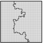
(a) Typical setup: a random curve is defined on a lattice approximation of $U$ and is connecting two boundary points $a$ and $b$.

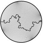
(b) The same random curve after a conformal transformation to $\mathbb{D}$ taking $a$ and $b$ to $-1$ and $+1$, respectively.

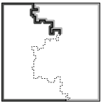
(c) Under the domain Markov property the curve conditioned on its beginning part has the same law as the one in the domain with the initial segment removed.

Figure 1: The assumptions of the main theorem are often easier to verify in the domain where the curve is originally defined (a) and the slit domains appearing as we trace the curve (c). Nevertheless, to set up the Loewner evolution we need to uniformize conformally to a fixed domain, e.g. the unit disc (b). Figure (c) illustrates the domain Markov property under which it is possible to verify the simpler “time $0$” condition (presented in this section) instead of its conditional versions (see Section 2.1.3).

Typically, the random curves we want to consider connect two boundary points $a,b\in\partial U$ in a simply connected domain $U$. Also it is possible to assume that the random curve is (almost surely) simple, because the curve is usually defined on a lattice with small but finite lattice mesh without “transversal” self-intersections. Therefore, by slightly perturbing the lattice and the curve it is possible to remove self-intersections. The main theorem of this paper involves the Loewner equation, and consequently the curves have to be either simple or non-self-traversing, i.e., curves that are limits of sequences of simple curves.

While we work with different domains $U$, we still prefer to restate our conclusions for a fixed domain. Thus we encode the domain $U$ and the curve end points $a,b\in\partial U$ by a conformal transformation $\phi$ from $U$ onto the unit disc $\mathbb{D}=\{z\in\mathbb{C}\;:\;|z|<1\}$. The domain $U=U(\phi)$ is then the domain of definition of $\phi$ and the points $a$ and $b$ are preimages $\phi^{-1}(-1)$ and $\phi^{-1}(1)$, respectively, if necessary define these in the sense of prime ends.

Because of the above reasons the first fundamental object in our study is a pair $(\phi,\mathbb{P})$ where $\phi$ is a conformal map and $\mathbb{P}$ is a probability measure on curves with the following restrictions: Given $\phi$ we define the domain $U=U(\phi)$ to be the domain of definition of $\phi$ and we require that $\phi$ is a conformal map from $U$ onto the unit disc $\mathbb{D}$. Therefore $U$ is a simply connected domain other than $\mathbb{C}$. We require also that $\mathbb{P}$ is supported on (a closed subset of)

$$\left\{\gamma\in X_{\mathrm{simple}}(U)\;:\;\begin{gathered}\text{the beginning and end point of}\\ \text{$\phi(\gamma)$ are $-1$ and $+1$, respectively}\end{gathered}\right\}.$$ (1)

The second fundamental object in our study is some collection $\Sigma$ of pairs $(\phi,\mathbb{P})$ satisfying the above restrictions.

Because the spaces involved are metrizable, when discussing convergence we may always think of $\Sigma$ as a sequence $((\phi_{n},\mathbb{P}_{n}))_{n\in\mathbb{N}}$. In applications, we often have in mind a sequence of interfaces for the same lattice model but with varying lattice mesh $\delta_{n}\searrow 0$: then each $\mathbb{P}_{n}$ is supported on curves defined on the $\delta_{n}$-mesh lattice. The main reason for working with the more abstract family compared to a sequence is to simplify the notation. If the set in (1) is non-empty, which is assumed, then there are in fact plenty of such curves, see Corollary 2.17 in [26].

We uniformize by a disk $\mathbb{D}$ to work with a bounded domain. As we show later in the paper, our conditions are conformally invariant, so the choice of a particular uniformization domain is not important.

For any $0<r<R$ and any point $z_{0}\in\mathbb{C}$, denote the annulus of radii $r$ and $R$ centered at $z_{0}$ by $A(z_{0},r,R)$:

$$A(z_{0},r,R)=\{z\in\mathbb{C}\;:\;r<|z-z_{0}|<R\}.$$ (2)

We call the quantity $(1/2\pi)\,\log\left(R/r\right)$ the modulus of the annulus $A(z_{0},r,R)$. The following definition makes speaking about crossing of annuli precise.

Definition 1.1.

For a curve $\gamma:[T_{0},T_{1}]\to\mathbb{C}$ and an annulus $A=A(z_{0},r,R)$, $\gamma$ is said to be a crossing of the annulus $A$ if both $\gamma(T_{0})$ and $\gamma(T_{1})$ lie outside $A$ and they are in the different components of $\mathbb{C}\setminus A$. A curve $\gamma$ is said to make a crossing of the annulus $A$ if there is a subcurve which is a crossing of $A$. A minimal crossing of the annulus $A$ is a crossing which doesn’t have genuine subcrossings.

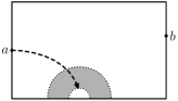
(a) Unforced crossing: the component of the annulus is not disconnecting $a$ and $b$. It is possible that the curve avoids the set. In this picture $A^{u}$ is the entire half-annulus.

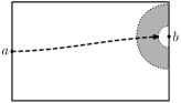
(b) Forced crossing: the component of the annulus disconnects $a$ and $b$ and does it in the way, that every curve connecting $a$ and $b$ has to cross the annulus at least once. In this picture $A^{u}$ is empty.

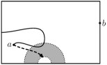
(c) There is an ambiguous case which resembles more either one of the previous two cases depending on the geometry. In this case the component of the annulus separates $a$ and $b$, but there are some curves from $a$ to $b$ in $U$ which don’t cross the annulus. In this picture $A^{u}$ is the small top part of the half-annulus.

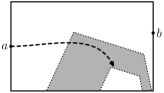
(d) Unforced crossing of a topological quadrilateral (quad): the quad is not disconnecting $a$ and $b$.

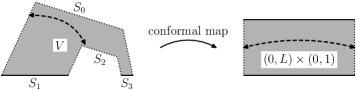
(e) The quads we consider have two of their sides on the boundary and two in the interior of the domain. We usually denote the sides by $S_{0},S_{2}\subset U$ and $S_{1},S_{3}\subset\partial U$. The set $V$ is the interior of the quad. There exists a unique number $L>0$ (and a unique conformal map) such that the quad can be mapped conformally onto the rectangle $(0,L)\times(0,1)$ so that the sides of the quad get mapped to the sides of the rectangle and $S_{0}$ gets mapped onto $\{0\}\times{}{[0,1]}$.

Figure 2: The general idea of Condition G2 is that an event of an unforced crossing has uniformly positive probability to fail. In the figures 2(a)–2(c) the solid line is the boundary of the domain, the dotted lines are the boundaries of the annulus and the dashed lines refer to the crossing event we are considering. The conformally invariant version of this is Condition C2 which is formulated using topological quadrilaterals. The figure 2(d) corresponds to the figure 2(a) in this latter setting.

We cannot require that crossing any fixed annulus has a small probability under $\mathbb{P}$: indeed, annuli centered at $a$ or at $b$ have to be crossed at least once. For that reason we introduce the following definition for a fixed simply connected domain $U$ and an annulus $A=A(z_{0},r,R)$ which is allowed to vary. If $\partial B(z_{0},r)\cap\partial U=\emptyset$ define $A^{u}=\emptyset$, otherwise

$$A^{u}=\left\{z\in U\cap A\,:\,\begin{gathered}\text{the connected component of $z$ in $U\cap A$}\\ \text{doesn't disconnect $a$ from $b$ in $U$}\end{gathered}\right\}.$$ (3)

This reflects the idea explained in Figure 2.

The main theorem is proven under a set of equivalent conditions. In this section, two simplified versions are presented. They are so called time $0$ conditions which imply the stronger conditional versions if our random curves satisfy the domain Markov property, cf. Figure 1(c). It should be noted that even in physically interesting situations the latter might fail, so the conditions presented in the section 2.1.3 should be taken as the true assumptions of the main theorem.

Condition G1.

The family $\Sigma$ is said to satisfy a geometric bound on an unforced crossing (at time zero) if there exists $C>1$ such that for any $(\phi,\mathbb{P})\in\Sigma$ and for any annulus $A=A(z_{0},r,R)$ with $0<C\,r\leq R$,

$$\mathbb{P}\left(\text{$\gamma$ makes a crossing of $A$ which is contained in $\overline{A^{u}}$}\,\right)\leq\frac{1}{2}.$$ (4)

We stress already at this point that the constant $1/2$ on the right-hand side of (4) or in similar bounds is arbitrary and could be replaced by any other constant strictly less than one. We will demonstrate this in Corollary 2.7.

A topological quadrilateral $Q=(V;S_{k},k=0,1,2,3)$ consists a domain $V$ which is homeomorphic to a square in a way that the boundary arcs $S_{k}$, $k=0,1,2,3$, are in counterclockwise order and correspond to the four edges of the square. There exists a unique positive $L$ and a conformal map from $Q$ onto a rectangle $[0,L]\times[0,1]$ mapping $S_{k}$ to the four edges of the rectangle with image of $S_{0}$ being $\{0\}\times[0,1]$. The number $L$ is called the modulus of (or the extremal length the curve family joining the opposite sides of) $Q$ and we will denote it by $m(Q)$.

We often consider a topological quadrilateral $Q=(V;S_{k},k=0,1,2,3)$ which is lying on the boundary in the sense that $S_{1}\cup S_{3}\subset\partial U$ while $S_{0}\cup S_{2}\subset U$ — this idea corresponds to the condition imposed when we defined $A^{u}$. For this type of topological quadrilateral we say that a curve $\gamma:[T_{0},T_{1}]\to\mathbb{C}$ crosses $Q$ in the domain $U$ if there is a subinterval $[t_{0},t_{1}]\subset[T_{0},T_{1}]$ such that $\gamma(t_{0},t_{1})\subset V$, but $\gamma[t_{0},t_{1}]$ intersects both $S_{0}$ and $S_{2}$. The other notions of Definition 1.1 are extended to the topological quadrilaterals in the same way. The following is the first conformally invariant version of our conditions, formulated in terms of topological quadrilaterals.

Condition C1.

The family $\Sigma$ is said to satisfy a conformal bound on an unforced crossing (at time zero) if there exists $M>0$ such that for any $(\phi,\mathbb{P})\in\Sigma$ and for any topological quadrilateral $Q$ with $V(Q)\subset U$, $S_{1}\cup S_{3}\subset\partial U$ and $m(Q)\geq M$

$$\mathbb{P}\left(\text{$\gamma$ makes a crossing of $Q$}\right)\leq\frac{1}{2}.$$ (5)

Remark 1.2.

In percolation type models of statistical physics including the random cluster models, this type of crossing events are the most central objects of study.

Remark 1.3.

Notice that depending on the point of view, either one of the conditions can appear stronger than the other one. In Condition G1 we require that the bound holds for all annuli with large modulus and simultaneously for all components of $A^{u}$, whereas in Condition C1 the bound holds for all topological quadrilaterals with large modulus and for its single (only) component. On the other hand, the set of topological quadrilaterals is bigger than the set of topological quadrilaterals $Q$ whose boundary arcs $S_{0}(Q)$ and $S_{2}(Q)$ are subsets of different boundary components of some annulus and $V(Q)$ is subset of that annulus. The latter set is the set of shapes relevant in Condition G1, at least naively speaking.

1.2 Main theorem

The main results of this article will be on the tightness of certain families of probability measures and on the convergence of probability measures in the weak sense. Hence let’s first recall the following definitions.

Definition 1.4.

Let $Y$ be a metric space and $\mathcal{B}_{Y}$ its Borel $\sigma$-algebra.

If $\Sigma_{0}$ is a collection of probability measures on $(Y,\mathcal{B}_{Y})$, then a random variable $f:Y\to\mathbb{R}$ is said to be tight or stochastically bounded in $\Sigma_{0}$ if and only if for each $\varepsilon>0$ there is $M>0$ such that $\mathbb{P}(|f|\leq M)\geq 1-\varepsilon$ for all $\mathbb{P}\in\Sigma_{0}$.

A collection $\Sigma_{0}$ of probability measures on $(Y,\mathcal{B}_{Y})$ is said to be tight if for each $\varepsilon>0$ there exists a compact set $K\subset Y$ so that $\mathbb{P}(K)\geq 1-\varepsilon$ for any $\mathbb{P}\in\Sigma_{0}$.

For the background in the weak convergence of probability measures the reader should see for example [5]. Prohorov’s theorem states that a family of probability measures is relatively compact if it is tight, see Theorem 5.1 in [5]. Moreover, in a separable and complete metric space relative compactness and tightness are equivalent.

Denote by $\phi\mathbb{P}$ the pushforward of $\mathbb{P}$ by $\phi$ defined by

$$(\phi\mathbb{P})(A)=\mathbb{P}(\phi^{-1}(A))$$ (6)

for any measurable $A\subset X_{\mathrm{simple}}(\mathbb{D})$. In other words $\phi\mathbb{P}$ is the law of the random curve $\phi(\gamma)$. Given a family $\Sigma$ as above, define the family of pushforward measures

$$\Sigma_{\mathbb{D}}=\left\{\phi\mathbb{P}\;:\;(\phi,\mathbb{P})\in\Sigma\right\}.$$ (7)

The family $\Sigma_{\mathbb{D}}$ consist of measures on the curves $X_{\mathrm{simple}}(\mathbb{D})$ connecting $-1$ to $1$.

Fix a conformal map

$$\Phi(z)=i\frac{z+1}{1-z}$$ (8)

which takes $\mathbb{D}$ onto the upper half-plane $\mathbb{H}=\{z\in\mathbb{C}\,:\,\operatorname{Im}z>0\}$. Note that if $\gamma$ is distributed according to $\mathbb{P}\in\Sigma_{\mathbb{D}}$, then $\tilde{\gamma}=\Phi(\gamma)$ is a simple curve in the upper half-plane slightly extending the definition of $X_{\mathrm{simple}}(\mathbb{H})$, namely, $\tilde{\gamma}$ is simple with $\tilde{\gamma}(0)=0\in\mathbb{R}$, $\tilde{\gamma}((0,1))\subset\mathbb{H}$ and $|\gamma(t)|\to\infty$ as $t\to 1$. Therefore by the results of Appendix A.1, if $\tilde{\gamma}$ is parametrized with the half-plane capacity, then it has a continuous driving term $W=W_{\gamma}:\mathbb{R}_{+}\to\mathbb{R}$. As a convention the driving term or process of a curve or a random curve in $\mathbb{D}$ means the driving term or process in $\mathbb{H}$ after the transformation $\Phi$ and using the half-plane capacity parametrization.

The following theorem and its reformulation, Proposition 3.1, are the main results of this paper. Note that the following theorem concerns with $\Sigma_{\mathbb{D}}$. The proof will be presented in Section 3. It is divided into three independent steps each in its own subsection and the actual proof is then presented in Section 3.5. See Section 2.1.3 for the exact assumptions of the theorem, namely, Condition G2. It should be noted that when the random curve has the domain Markov property, which is schematically defined in Figure 1(c), Condition G1 implies Condition G2, which is merely a conditional version of Condition G1.

Theorem 1.5.

If the family $\Sigma$ of probability measures satisfies Condition G2, then the family $\Sigma_{\mathbb{D}}$ is tight and therefore relatively compact in the topology of the weak convergence of probability measures on $(X,\mathcal{B}_{X})$. Furthermore if $\mathbb{P}_{n}\in\Sigma_{\mathbb{D}}$ is converging weakly and the limit is denoted by $\mathbb{P}^{*}$ then the following statements hold $\mathbb{P}^{*}$ almost surely

1. the point $1$ is not a double point, i.e., $\gamma(t)=1$ only if $t=1$,

2. there exists $\beta>0$ such that $\gamma$ has a Hölder continuous parametrization for the Hölder exponent $\beta$,

3. the tip $\gamma(t)$ of the curve lies on the boundary of the connected component of $\mathbb{D}\setminus\gamma[0,t]$ containing $1$ (having the point $1$ on its boundary), for all $t$,

4. if $\hat{K}_{t}$ is the hull of $\Phi(\gamma[0,t])$, then the capacity $\mathrm{cap}_{\mathbb{H}}(\hat{K}_{t})\to\infty$ as $t\to 1$

5. for any parametrization of $\gamma$ the capacity $t\mapsto\mathrm{cap}_{\mathbb{H}}(\hat{K}_{t})$ is strictly increasing and if $(K_{t})_{t\in\mathbb{R}_{+}}$ is $(\hat{K}_{t})_{t\in[0,1)}$ reparametrized with capacity, then the corresponding $g_{t}$ satisfies the Loewner equation with a driving process $(W_{t})_{t\in\mathbb{R}_{+}}$ which is Hölder continuous for any exponent $\alpha<1/2$.

Furthermore, there exist constants $\varepsilon>0$ and $C>0$ such that

$$\mathbb{E}^{*}\left[\exp\left(\varepsilon\max_{s\in[0,t]}|W_{s}|/\sqrt{t}\right)\right]\leq C$$ (9)

for any $t>0$. Here $\mathbb{E}^{*}$ denotes the expected value with respect to $\mathbb{P}^{*}$.

Remark 1.6.

Note that the claims (i)–(iv) don’t depend on the parameterization.

The following corollary clarifies the relation between the convergence of random curves and the convergence of their driving processes. For instance, it shows that if the driving processes of Loewner chains satisfying Condition G2 converge, also the limiting Loewner chain is generated by a curve. In the statement of the result we assume that $\mathbb{H}$ is endowed with a bounded metric, for instance, the one inherited from the Riemann sphere. Another possibility is to map $\mathbb{H}$ onto a bounded domain such as $\mathbb{D}$.

Corollary 1.7.

Suppose that $(W^{(n)})_{n\in\mathbb{N}}$ is a sequence of driving processes of random Loewner chains that are generated by simple random curves $(\gamma^{(n)})_{n\in\mathbb{N}}$ in $\mathbb{H}$, satisfying Condition G2. Suppose also that $(\gamma^{(n)})_{n\in\mathbb{N}}$ are parametrized by capacity. Then

• $(W^{(n)})_{n\in\mathbb{N}}$ is tight in the metrizable space of continuous functions on $[0,\infty)$ with the topology of uniform convergence on the compact subsets of $[0,\infty)$.

• $(\gamma^{(n)})_{n\in\mathbb{N}}$ is tight in the space of curves $X$.

• $(\gamma^{(n)})_{n\in\mathbb{N}}$ is tight in the metrizable space of continuous functions on $[0,\infty)$ with the topology of uniform convergence on the compact subsets of $[0,\infty)$.

Moreover, if the sequence converges in any of the topologies above it also converges in the two other topologies and the limits agree in the sense that the limiting random curve is driven by the limiting driving process.

The space $C([0,\infty))$ is metrizable, since a metric on it is given, for example, by

$$\mathrm{d}(f,g)=\sum_{n=0}^{\infty}2^{-n}\min\{1,\sup\{|f(t)-g(t)|\,:\,t\in[0,2^{n}]\}\}.$$

It is understood that $a=\gamma^{(n)}(0)$ and $b=\infty$ in the definition of $A^{u}$.

For the next corollary let’s define the space of open curves by identifying in the set of continuous maps $\gamma:(0,1)\to\mathbb{C}$ different parametrizations. The topology will be given by the convergence on the compact subsets of $(0,1)$. See also Section 3.6. It is necessary to consider open curves since in rough domains nothing guarantees that there are curves starting from a given boundary point or prime end.

We say that $(U_{n},a_{n},b_{n})$, $n\in\mathbb{N}$, converges to $(U,a,b)$ in the Carathéodory sense if there exist conformal and onto mappings $\psi_{n}:\mathbb{D}\to U_{n}$ and $\psi:\mathbb{D}\to U$ such that they satisfy $\psi_{n}(-1)=a_{n}$, $\psi_{n}(+1)=b_{n}$, $\psi(-1)=a$ and $\psi(+1)=b$ (possibly defined as prime ends) and such that $\psi_{n}$ converges to $\psi$ uniformly in the compact subsets of $\mathbb{D}$ as $n\to\infty$. Note that this limit is not necessarily unique as a sequence $(U_{n},a_{n},b_{n})$ can converge to different limits for different choices of $\psi_{n}$. However if know that $(U_{n},a_{n},b_{n})$, $n\in\mathbb{N}$, converges to $(U,a,b)$, then $\psi(0)\in U_{n}$ for large enough $n$ and $U_{n}$ converges to $U$ in the usual sense of Carathéodory kernel convergence with respect to the point $\psi(0)$. For the definition see Section 1.4 of [26].

The next corollary shows that if we have a converging sequence of random curves in the sense of Theorem 1.5 and if they are supported on domains which converge in the Carathéodory sense, then the limiting random curve is supported on the limiting domain. Note that the Carathéodory kernel convergence allows that there are deep fjords in $U_{n}$ which are “cut off” as $n\to\infty$. One can interpret the following corollary to state that with high probability the random curves don’t enter any of these fjords. This is a desired property of the convergence.

Corollary 1.8.

Suppose that the sequence $(U_{n},a_{n},b_{n})$ converges to $(U^{*},a^{*},b^{*})$ in the Carathéodory sense (here $a^{*}$, $b^{*}$ are possibly defined as prime ends) and suppose that $(\phi_{n})_{n\geq 0}$ are conformal maps such that $U_{n}=U(\phi_{n}),a_{n}=a(\phi_{n}),b_{n}=b(\phi_{n})$ and $\lim\phi_{n}=\phi^{*}$ for which $U^{*}=U(\phi^{*}),a^{*}=a(\phi^{*}),b=b(\phi^{*})$. Let $\hat{U}=U^{*}\setminus(V_{a}\cup V_{b})$ where $V_{a}$ and $V_{b}$ are some neighborhoods of $a$ and $b$, respectively, and set $\hat{U}_{n}=\phi_{n}^{-1}\circ\phi(\hat{U})$. If $(\phi_{n},\mathbb{P}_{n})_{n\geq 0}$ satisfy Condition G2 and $\gamma^{(n)}$ has the law $\mathbb{P}_{n}$, then $\gamma^{(n)}$ restricted to $\hat{U}_{n}$ has a weakly converging subsequence in the topology of $X$, the laws for different $\hat{U}$ are consistent so that it is possible to define a random curve $\gamma$ on the open interval $(0,1)$ such that the limit for $\gamma^{(n)}$ restricted to $\hat{U}_{n}$ is $\gamma$ restricted to the closure of $\hat{U}$. In particular, almost surely the limit of $\gamma^{(n)}$ is supported on open curves of $U^{*}$ and doesn’t enter $(\limsup U_{n})\setminus\overline{U}^{*}$.

Here we define $\limsup A_{n}$ for a sequence of sets $A_{n}\subset\mathbb{C}$ to be the set

$$\left\{x\in\mathbb{C}\,:\,\exists\text{ increasing }n_{k}\in\mathbb{N}\text{ and }x_{k}\in A_{n_{k}}\text{ sequences s.t. }\lim_{k\to\infty}x_{k}=x\right\}=\bigcap_{m=1}^{\infty}\overline{\bigcup_{n=m}^{\infty}A_{n}}\;.$$

1.3 The principal application of the main theorem

The results of this paper (Corollary 1.8 and Proposition 4.3) together with [37], [11] and [9] are used in [10] to establish the following (strong) convergence result for the Ising model interfaces. For the exact setting consult Section 4.1.

Theorem 1.9 (Chelkak–Duminil-Copin–Hongler–Kemppainen–Smirnov [10]).

Let $U$ be a bounded simply connected domain with two distinct boundary points $a,b$ (possibly defined as prime ends).

• (Convergence of spin Ising interfaces) Consider the interface $\gamma_{\delta}$ in the critical spin Ising model with Dobrushin boundary conditions on $(U_{\delta},a_{\delta},b_{\delta})$. The law of $\gamma_{\delta}$ converges weakly, as $\delta\to 0$, to the chordal Schramm-Loewner Evolution SLE$(\kappa)$ running from $a$ to $b$ in $U$ with $\kappa=3$.

• (Convergence of FK Ising interfaces). Consider the interface $\gamma_{\delta}$ in the critical FK Ising model with Dobrushin boundary conditions on $(U_{\delta},a_{\delta},b_{\delta})$. The law of $\gamma_{\delta}$ converges weakly, as $\delta\to 0$, to the chordal Schramm-Loewner Evolution SLE$(\kappa)$ running from $a$ to $b$ in $U$ with $\kappa=16/3$.

The above result is based on a standard approach for proving convergence. First we show precompactness of the sequence so that it has subsequential limits. Then we show that those limits are independent of the subsequence (uniqueness). It follows that the whole sequence converges to this unique limit. The results of the present article are sufficient to cover the entire precompactness part, but this work also gives some required tools for the uniqueness part.

The uniqueness part is based on finding an observable which has a well-behaved scaling limit. A typical observable is a solution of a discrete boundary value problem, e.g., the observable could be a discrete harmonic function with prescribed boundary values and defined on the same or related graph as the interface. There needs to be a strong connection between the observable and the interface so that the observable is a martingale with respect to the information generated by the growing curve.

Unfortunately, the observables satisfying all the required properties have so far been found in only a few cases.

In the article [10] Condition G2 is verified for the spin Ising model using the results of [9]. In Section 4.2 below, we give its alternative derivation using only the observable results of [11], thus giving a new proof of Theorem 1.9, independent of [9] and using only [11] and the “martingale characterization” from [10].

Moreover, our proof indicates that in general, a non-degenerate martingale observable should suffice to verify Condition G2. Another known example of such an approach is its verification for the harmonic observable which we sketch in Section 4.4.

1.4 An application to the continuity of SLE

This section is devoted to an application of Theorem 1.5.

Consider SLE$(\kappa)$, $\kappa\in[0,8)$, for different values of $\kappa$. For an introduction to Schramm–Loewner evolution see Appendix A.1 below and [20]. The driving processes of the different SLEs can be given in the same probability space in the obvious way by using the same standard Brownian motion for all of them. A natural question is to ask whether or not SLE is as a random curve continuous in the parameter $\kappa$. See also [17], where it is proved that SLE is continuous in $\kappa$ for small and large $\kappa$ in the sense of almost sure convergence of the curves when the driving processes are coupled in the way given above. We will prove the following theorem using Corollary 1.7.

Theorem 1.10.

Let $\gamma^{[\kappa]}(t)$, $t\in[0,\infty)$, be SLE$(\kappa)$ parametrized by capacity. Suppose that $\kappa\in[0,8)$ and $\kappa_{n}\to\kappa$ as $n\to\infty$. Then as $n\to\infty$, the law of $\gamma^{[\kappa_{n}]}$ converges weakly to the law of $\gamma^{[\kappa]}$ in the topology of uniform convergence on the compact subsets of $[0,\infty)$.

We’ll present the proof here since it is independent of the rest of the paper except that it relies on Corollary 1.7, Proposition 2.6 (equivalence of geometric and conformal conditions) and Remark 2.9 (on the domain Markov property). The reader can choose to read these parts before reading this proof.

Notice that SLE$(\kappa)$ is not simple when $\kappa>4$. Therefore we need to slightly extend the setting of this paper to be able to use it in the proof of Theorem 1.10. The assumption that the random curves are simple is used essentially only to guarantee that they are Loewner chains with continuous driving processes. Also that assumption makes it less cumbersome to talk about the tip of the curve and whether or not some set separates the tip and the target points from each other, but this is not a problem in the general case either, since we can always use conformal mappings and resolve the question in some Jordan domain. As a consequence, no extra difficulties arise and we can work with SLE$(\kappa)$ as if they were simple curves.

Proof.

Let $\kappa_{0}\in[0,8)$. First we verify that the family consisting of SLE$(\kappa)$s on $\mathbb{D}$, say, where $\kappa$ runs over the interval $[0,\kappa_{0}]$, satisfies Condition G2. Since SLE_κ has the conformal domain Markov property, it is enough to verify Condition C1. More specifically, it is enough to show that there exists $M>0$ such that if $Q=(V,S_{0},S_{1},S_{2},S_{3})$ is a topological quadrilateral with $m(Q)\geq M$ such that $V\subset\mathbb{H}$, $S_{k}\subset\mathbb{R}_{+}\mathrel{\mathop{:}}=[0,\infty)$ for $k=1,3$ and $S_{2}$ separates $S_{0}$ from $\infty$ in $\mathbb{H}$, then

$$\mathbb{P}(\text{SLE$(\kappa)$ intersects }S_{0})\leq\frac{1}{2}$$ (10)

for any $\kappa\in[0,\kappa_{0}]$.

Suppose that $M>0$ is large and $Q$ satisfies $m(Q)\geq M$. Let $Q^{\prime}=(V^{\prime};S_{0}^{\prime},S_{2}^{\prime})$ be the doubly connected domain where $V^{\prime}$ is the interior of the closure of $V\cup V^{*}$, $V^{*}$ is the mirror image of $V$ with respect to the real axis, and $S_{0}^{\prime}$ and $S_{2}^{\prime}$ are the inner and outer boundary of $V^{\prime}$, respectively. Then the modulus (or extremal length) of $Q^{\prime}$, which is defined as the extremal length of the curve family connecting $S_{0}^{\prime}$ and $S_{2}^{\prime}$ in $V^{\prime}$ (for the definition see Chapter 4 of [1]), is given by $m(Q^{\prime})=m(Q)/2$.

Let $x=\min(\mathbb{R}\cap S_{0}^{\prime})>0$ and $r=\max\{|z-x|\,:\,z\in S_{0}^{\prime}\}>0$. Then $Q^{\prime}$ is a doubly connected domain which separates $x$ and a point on $\{z\,:\,|z-x|=r\}$ from $\{0,\infty\}$. By Theorem 4.7 of [1], of all the doubly connected domains with this property, the complement of $(-\infty,0]\cup[x,x+r]$ has the largest modulus. By the equation 4.21 of [1],

$$\exp(2\pi\,m(Q^{\prime}))\leq 16\left(\frac{x}{r}+1\right)$$ (11)

which implies that $r\leq\rho x$ where

$$\rho=\left(\frac{1}{16}\exp(\pi M)-1\right)^{-1}$$ (12)

which can be as small as we like by choosing $M$ large.

If SLE$(\kappa)$ crosses $Q$ then it necessarily intersects $\overline{B(x,r)}$. By the scale invariance of SLE$(\kappa)$

$$\mathbb{P}(\text{SLE$(\kappa)$ intersects }S_{0})\leq\mathbb{P}\left(\text{SLE$(\kappa)$ intersects }\overline{B(1,\rho)}\right).$$ (13)

Now by standard arguments [27], the right hand side can be made less than $1/2$ for $\kappa\in[0,\kappa_{0}]$ and $0<\rho\leq\rho_{0}$ where $\rho_{0}>0$ is suitably chosen constant.

Denote the driving process of $\gamma^{[\kappa]}$ by $W^{[\kappa]}$. If $\kappa_{n}\to\kappa\in[0,8)$, then obviously $W^{[\kappa_{n}]}$ converges weakly to $W^{[\kappa]}$. Hence by Corollary 1.7 also $\gamma^{[\kappa_{n}]}$ converges weakly to some $\tilde{\gamma}$ whose driving process is distributed as $W^{[\kappa]}$. That is, $\gamma^{[\kappa_{n}]}$ converges weakly to $\gamma^{[\kappa]}$ as $n\to\infty$ provided that $\kappa_{n}\to\kappa$ as $n\to\infty$. ∎

1.5 Structure of this paper

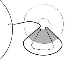
(a) When the radius of the inner circle goes to zero, the dashed line is no longer visible from a faraway reference point. If such an event has positive probability for the limiting measure, then the Loewner equation doesn’t describe the whole curve.

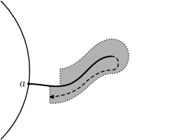
(b) Longitudinal crossing of an arbitrarily thin tube of fixed length along the curve or the boundary violates the local growth needed for the continuity of the Loewner driving term.

Figure 3: In the proof of Theorem 1.5, the regularity of random curves is established by establishing a probability upper bound on multiple crossings and excluding two unwanted scenarios presented in this figure.

In Section 2, the general setup of this paper is presented. Four conditions are stated and shown to be equivalent. Any one of them can be taken as the main assumption for Theorem 1.5.

The proof of Theorem 1.5 is presented in Section 3. The proof consists of three parts: the first one is the existence of regular parametrizations of the random curves and the second and third steps are described in Figure 3. The relevant condition is verified for a list of random curves arising from statistical mechanics models in Section 4.

2 The space of curves and equivalence of conditions

2.1 The space of curves and conditions

2.1.1 The space of curves

We follow the setup of Aizenman and Burchard’s paper [2]: planar curves are continuous mappings from $[0,1]$ to $\mathbb{C}$ modulo reparameterizations. Let

$$C^{\prime}=\left\{f\in C\left([0,1],\mathbb{C}\right)\,:\,\begin{gathered}\text{either $f$ is not constant on any subinterval of $[0,1]$}\\ \text{or $f$ is constant on $[0,1]$}\end{gathered}\right\}.$$

It is also possible to work with the whole space $C\left([0,1],\mathbb{C}\right)$, but the next definition is easier for $C^{\prime}$. Define an equivalence relation $\sim$ in $C^{\prime}$ so that $f_{1}\sim f_{2}$ if they are related by an increasing homeomorphism $\psi:[0,1]\to[0,1]$ with $f_{2}=f_{1}\circ\psi$. The reader can check that this defines an equivalence relation. The mapping $f_{1}\circ\psi$ is said to be a reparameterization of $f_{1}$ or that $f_{1}$ is reparameterized by $\psi$.

Note that these parameterizations are, in a sense, arbitrary and are in general different from the Loewner parameterization which we are going to construct.

Denote the equivalence class of $f$ by $[f]$. The set of all equivalence classes

$$X=\left\{[f]:f\in C^{\prime}\right\}$$

is called the space of curves. Make $X$ a metric space by setting

$$\mathrm{d}_{X}([f],[g])=\inf\{\|f_{0}-g_{0}\|_{\infty}:f_{0}\in[f],g_{0}\in[g]\}.$$ (14)

It is easy to see that this is a metric, see e.g. [2]. The space $X$ with the metric $\mathrm{d}_{X}$ is complete and separable reflecting the same properties of $C\left([0,1],\mathbb{C}\right)$. And for the same reason as $C\left([0,1],\mathbb{C}\right)$ is not compact neither is $X$.

Define two subspaces, the space $X_{\mathrm{simple}}$ of simple curves and the space $X_{0}$ of curves with no self-crossings by

$$X_{\mathrm{simple}} =\left\{[f]:f\in C^{\prime},f\textrm{ injective}\right\}$$

$$X_{0} =\overline{X_{\mathrm{simple}}}$$

Note that $X_{0}\subsetneq X$ since there exists $\gamma_{0}\in X\setminus X_{\mathrm{simple}}$ with positive distance to $X_{\mathrm{simple}}$. For example, such is the broken line passing through points $-1,1,i$ and $-i$ which has a double point which is stable under small perturbations.

What do the curves in $X_{0}$ look like? Roughly speaking, they may touch themselves and have multiple points, but they can have no “transversal” self-intersections. For example, the broken line through points $-1,1,i,0,-1+i$, also has a double point at $0$, but it can be removed by small perturbations. Also, every passage through the double point separates its neighborhood into two components, and every other passage is contained in (the closure) of one of those. See also Figure 4.

Figure 4: In this example the options 1 and 2 are possible so that the resulting curve in the class $X_{0}$. If the curve continues along $3$ it doesn’t lie in $X_{0}$, namely, there is no sequence of simple curves converging to that curve.

Given a domain $U\subset\mathbb{C}$ define $X(U)$ as the closure of $\{[f]:f\in C^{\prime},f[0,1]\subset U\}$ in $(X,\mathrm{d}_{X})$. Define also $X_{0}(U)$ as the closure of the set of simple curves in $X(U)$. The notation $X_{\mathrm{simple}}(U)$ we reserve for

$$X_{\mathrm{simple}}(U)=\left\{[f]:f\in C^{\prime},f\big{(}(0,1)\big{)}\subset U,f\textrm{ injective}\right\},$$

so the end points of such curves may lie on the boundary. Note that the closure of $X_{\mathrm{simple}}(U)$ is still $X_{0}(U)$.

Use also notation $X_{\mathrm{simple}}(U,a,b)$ for curves in $X_{\mathrm{simple}}(U)$ whose end points are $\gamma(0)=a$ and $\gamma(1)=b$. We will quite often consider some reference sets as $X_{\mathrm{simple}}(\mathbb{D},-1,+1)$ and $X_{\mathrm{simple}}(\mathbb{H},0,\infty)$ where the latter can be understood by extending the above definition to curves defined on the Riemann sphere, say.

We will often use the letter $\gamma$ to denote elements of $X$, i.e. a curve modulo reparameterizations. Note that topological properties of the curve (such as its endpoints or passages through annuli or its locus $\gamma[0,1]$) as well as metric ones (such as dimension or length) are independent of parameterization. When we want to put emphasis on the locus, we will be speaking about Jordan curves or arcs, usually parameterized by the open unit interval $(0,1)$.

Denote by $\mathrm{Prob}(X)$ the space of probability measures on $X$ equipped with the Borel $\sigma$-algebra $\mathcal{B}_{X}$ and the weak-$*$ topology induced by continuous functions (which we will call weak for simplicity). Suppose that $\mathbb{P}_{n}$ is a sequence of measures in $\mathrm{Prob}(X)$.

If for each $n$, $\mathbb{P}_{n}$ is supported on a closed subset of $X_{\mathrm{simple}}$ (which for discrete curves can be assumed without loss of generality) and if $\mathbb{P}_{n}$ converges weakly to a probability measure $\mathbb{P}$, then $1=\limsup_{n}\mathbb{P}_{n}(X_{0})\leq\mathbb{P}(X_{0})$ by general properties of the weak convergence of probability measures [5]. Therefore $\mathbb{P}$ is supported on $X_{0}$ but in general it doesn’t have to be supported on $X_{\mathrm{simple}}$.

2.1.2 Comment on the probability structure

Suppose $\mathbb{P}$ is supported on $D\subset X(\mathbb{C})$ which is a closed subset of $X_{\mathrm{simple}}(\mathbb{C})$. Consider some measurable map $\chi:D\to C([0,\infty),\mathbb{C})$ so that $\chi(\gamma)$ is a parametrization of $\gamma$. If necessary $\chi$ can be continued to $D^{c}$ by setting $\chi=0$ there.

Let $\pi_{t}$ be the natural projection from $C([0,\infty),\mathbb{C})$ to $C([0,t],\mathbb{C})$. Define a $\sigma$-algebra

$$\mathcal{F}_{t}^{\chi,0}=\sigma(\pi_{s}\circ\chi,0\leq s\leq t)\leavevmode\nobreak\ ,$$

and make it right continuous by setting $\mathcal{F}_{t}^{\chi}=\bigcap_{s>t}\mathcal{F}_{s}^{\chi,0}$.

For a moment denote by $(\tau,\hat{\tau})$ for given $\gamma,\hat{\gamma}\in D$ the maximal pair of times such that $\chi(\gamma)|_{[0,\tau]}$ is equal to $\chi(\hat{\gamma})|_{[0,\hat{\tau}]}$ in $X$, that is, equal modulo a reparameterization. We call $\chi$ a good parametrization of the curve family $D$, if for each $\gamma,\hat{\gamma}\in D$, $\tau=\hat{\tau}$ and $\chi(\gamma,t)=\chi(\hat{\gamma},t)$ for all $0\leq t\leq\tau$.

Each reparameterization from a good parametrization to another can be represented as stopping times $T_{u}$, $u\geq 0$. From this it follows that the set of stopping times is the same for every good parametrization. We will use simply the notation $\gamma[0,t]$ to denote the $\sigma$-algebra $\mathcal{F}_{t}^{\chi}$. The choice of a good parametrization $\chi$ is immaterial since all the events we will consider are essentially reparameterization invariant. But to ease the notation it is useful to always have some parametrization in mind.

Often there is a natural choice for the parametrization. For example, if we are considering paths on a lattice, then the probability measure is supported on polygonal curves. In particular, the curves are piecewise smooth and it is possible to use the arc length parametrization, i.e. $|\gamma^{\prime}(t)|=1$. One of the results in this article is that given the hypothesis, which is described next, it is possible to use the capacity parametrization of the Loewner equation. Both the arc length and the capacity are good parameterizations.

The following lemma is implied by the above definitions.

Lemma 2.1.

If $A\subset\mathbb{C}$ is a non-empty, closed set, then $\tau_{A}=\inf\{t\geq 0\,:\,\chi(\gamma,t)\in A\}$ is a stopping time.

Remark 2.2.

The stopping times we need in the proof of the main theorem are always explicitly of this type.

2.1.3 Four equivalent conditions

Recall the general setup: we are given a collection $(\phi,\mathbb{P})\in\Sigma$ where the conformal map $\phi$ contains also the information about the domain $(U,a,b)=(U(\phi),a(\phi),b(\phi))$ and $\mathbb{P}$ is a probability measure on $X_{\mathrm{simple}}(U,a,b)$. Furthermore, we assume that each $\gamma$, which is distributed according to $\mathbb{P}$, has some suitable parametrization.

For given domain $U$ and for given simple (random) curve $\gamma$ on $U$, we always define $U_{\tau}=U\setminus\gamma[0,\tau]$ for each (random) time $\tau$. We call $U_{\tau}$ as the domain at time $\tau$.

Definition 2.3.

For a fixed domain $(U,a,b)$ and for fixed simple (random) curve in $U$ starting from $a$, define for any annulus $A=A(z_{0},r,R)$ and for any (random) time $\tau\in[0,1]$, $A^{u}_{\tau}=\emptyset$ if $\partial B(z_{0},r)\cap\partial U_{\tau}=\emptyset$ and

$$A^{u}_{\tau}=\left\{z\in U_{\tau}\cap A\,:\,\begin{gathered}\text{the connected component of $z$ in $U_{\tau}\cap A$}\\ \text{doesn't disconnect $\gamma(\tau)$ from $b$ in $U_{\tau}$}\end{gathered}\right\}$$ (15)

otherwise. A connected set $C$ disconnects $\gamma(\tau)$ from $b$ if it disconnects some neighborhood of $\gamma(\tau)$ from some neighborhood of $b$ in $U_{\tau}$. If $\gamma[\tau,1]$ contains a crossing of $A$ which is contained in $A_{\tau}^{u}$, we say that $\gamma$ makes an unforced crossing of $A$ in $U_{\tau}$ (or an unforced crossing of $A$ observed at time $\tau$). The set $A_{\tau}^{u}$ is said to be avoidable at time $\tau$.

Remark 2.4.

Neighborhoods are needed here only to incorporate the fact that $\gamma(t)$ and $b$ are boundary points.

The first two of the four equivalent conditions are geometric, asking an unforced crossing of an annulus to be unlikely uniformly in terms of the modulus.

Condition G2.

The family $\Sigma$ is said to satisfy a geometric bound on an unforced crossing if there exists $C>1$ such that for any $(\phi,\mathbb{P})\in\Sigma$, for any stopping time $0\leq\tau\leq 1$ and for any annulus $A=A(z_{0},r,R)$ where $0<C\,r\leq R$,

$$\mathbb{P}\big{(}\big{.}\gamma[\tau,1]\textrm{ makes a crossing of }A\text{ which is contained in }\overline{A^{u}_{\tau}}\,\big{|}\,\gamma[0,\tau]\big{)}<\frac{1}{2}.$$ (16)

Condition G3.

The family $\Sigma$ is said to satisfy a geometric power-law bound on an unforced crossing if there exist $K>0$ and $\Delta>0$ such that for any $(\phi,\mathbb{P})\in\Sigma$, for any stopping time $0\leq\tau\leq 1$ and for any annulus $A=A(z_{0},r,R)$ where $0<r\leq R$,

$$\mathbb{P}\big{(}\big{.}\gamma[\tau,1]\textrm{ makes a crossing of }A\text{ which is contained in }\overline{A^{u}_{\tau}}\,\big{|}\,\gamma[0,\tau]\big{)}\leq K\left(\frac{r}{R}\right)^{\Delta}.$$ (17)

Let $Q\subset U_{t}$ be a topological quadrilateral, i.e. an image of the square $(0,1)^{2}$ under a homeomorphism $\psi$. Define the “sides” $\partial_{0}Q$, $\partial_{1}Q$, $\partial_{2}Q$, $\partial_{3}Q$, as the “images” of

$$\left\{0\right\}\times(0,1),\quad(0,1)\times\left\{0\right\},\quad\left\{1\right\}\times(0,1),\quad(0,1)\times\left\{1\right\}$$

under $\psi$. For example, we set

$$\partial_{0}Q:=\lim_{\epsilon\to 0}\mathrm{Clos}\left(\psi\left(\;(0,\epsilon)\times(0,1)\;\right)\right).$$

We consider $Q$ such that two opposite sides $\partial_{1}Q$ and $\partial_{3}Q$ are contained in $\partial U_{t}$. A crossing of $Q$ is a curve in $U_{t}$ connecting two opposite sides $\partial_{0}Q$ and $\partial_{2}Q$. The latter without loss of generality (just perturb slightly) we assume to be smooth curves of finite length inside $U_{t}$. Call $Q$ avoidable if it doesn’t disconnect $\gamma(t)$ and $b$ inside $U_{t}$.

Condition C2.

The family $\Sigma$ is said to satisfy a conformal bound on an unforced crossing if there exists a constant $M>0$ such that for any $(\phi,\mathbb{P})\in\Sigma$, for any stopping time $0\leq\tau\leq 1$ and any avoidable quadrilateral $Q$ of $U_{\tau}$, such that the modulus $m(Q)$ is larger than $M$

$$\mathbb{P}\big{(}\big{.}\gamma[\tau,1]\textrm{ crosses }Q\,\big{|}\,\gamma[0,\tau]\big{)}\leq\frac{1}{2}.$$ (18)

Remark 2.5.

In the condition above, the quadrilateral $Q$ depends on $\gamma[0,\tau]$, but this does not matter, as we consider all such quadrilaterals. A possible dependence on $\gamma[0,\tau]$ ambiguity can be addressed by mapping $U_{t}$ to a reference domain and choosing quadrilaterals there. See also Remark 2.10.

Condition C3.

The family $\Sigma$ is said to satisfy a conformal power-law bound on an unforced crossing if there exist constants $K$ and $\epsilon$ such that for any $(\phi,\mathbb{P})\in\Sigma$, for any stopping time $0\leq\tau\leq 1$ and any avoidable quadrilateral $Q$ of $U_{\tau}$

$$\mathbb{P}\big{(}\big{.}\gamma[\tau,1]\textrm{ crosses }Q\,\big{|}\,\gamma[0,\tau]\big{)}\leq K\,\exp(-\epsilon\,m(Q)).$$ (19)

Proposition 2.6.

The four conditions G2, G3, C2 and C3 are equivalent and conformally invariant.

This proposition is proved below in Section 2.2. Equivalence of conditions immediately implies the following

Corollary 2.7.

The constant $1/2$ in Conditions G2 and C2 can be replaced by any other from $(0,1)$.

2.1.4 Remarks concerning the conditions

Remark 2.8.

Conditions G2 and G3 could be described as being geometric since they involve crossing of fixed shape. Conditions C2 and C3 are conformally invariant because they are formulated using the modulus, i.e., the extremal length which is a conformally invariant quantity. The conformal invariance in Proposition 2.6 means for example, that if Condition G2 holds with a constant $C>1$ for $(\phi,\mathbb{P})$ defined in $U$ and if $\psi:U\to U^{\prime}$ is conformal and onto, then Condition G2 holds for $(\phi\circ\psi^{-1},\psi\mathbb{P})$ with a constant $C^{\prime}>1$ which depends only on the constant $C$ but not on $(\phi,\mathbb{P})$ or $\psi$.

Remark 2.9.

To formulate the domain Markov property with an appropriate set of stopping times, let’s suppose that $\Sigma$ is a collection of pairs $(\phi_{n}^{U,a,b},\mathbb{P}_{n}^{U,a,b})$ where $n\in\mathbb{N}$ refers to the lattice mesh $\delta_{n}$ which tends to zero as $n$ tends to infinity, $U$ is a simply connected domain whose boundary is a discrete curve (broken line) on the lattice with mesh $\delta_{n}$ and $a$ and $b$ are lattice points on the boundary of the domain and as usual $\phi_{n}^{U,a,b}$ is a conformal map taking $U,a,b$ onto $\mathbb{D},-1,1$. If for any stopping time $\tau$, such that $\gamma(\tau)$ is almost surely a lattice point, it holds that

$$\mathbb{P}^{U,a,b}_{n}\left(\left.\gamma|_{[\tau,1]}\in\cdot\,\right|\,\gamma|_{[0,\tau]}\right)=\mathbb{P}^{U\setminus\gamma[0,\tau],\gamma(\tau),b}_{n},$$

then the random curve or $\Sigma$ is said to have the domain Markov property. This property could be formulated more generally so that if $\mathbb{P}$ is a probability measure such that $(\phi,\mathbb{P})\in\Sigma$ for some $\phi$, then for any stopping time $\tau$, $\mathbb{P}\left(\left.\gamma|_{[\tau,1]}\in\cdot\,\right|\,\gamma|_{[0,\tau]}\right)$ is equal to some probability measure $\mathbb{P}^{\prime}$ such that $(\phi^{\prime},\mathbb{P}^{\prime})\in\Sigma$ for some $\phi^{\prime}$.

When the domain Markov property holds, the “time zero conditions” G1 and C1 are sufficient for Conditions G2 and C2, respectively.

Remark 2.10.

Our conditions impose an estimate on conditional probability, which is hence satisfied almost surely. By taking a countable dense set of round annuli (or of topological rectangles), we see that it does not matter whether we require the estimate to hold separately for any given annulus almost surely; or to hold almost surely for every annulus. The same argument applies to topological rectangles.

Remark 2.11.

Suppose now that the random curve $\gamma$ is an interface in a statistical physics model with two possible states at each site, say, blue and red. In that case $U$ will be a simply connected domain formed by entire faces of some lattice, say, hexagonal lattice, $a,b\in\partial U$ are boundary points, the faces next to the arc $ab$ are colored blue and next to the arc $ba$ red and $\gamma$ is the interface between the blue cluster of $ab$ (connected set of blue faces) and the red cluster of $ba$.

In this case under positive association (e.g. observing blue faces somewhere increases the probability of observing blue sites elsewhere) the sufficient condition implying Condition G2 is uniform upper bound for the probability of the crossing event of an annular sector with alternating boundary conditions (red–blue–red–blue) on the four boundary arcs (circular–radial–circular–radial) by blue faces. For more detail, see Section 4.1.6.

2.2 Equivalence of the geometric and conformal conditions

In this section we prove Proposition 2.6 about equivalence of geometric and conformal conditions. We start with recalling the notion of Beurling’s extremal length and then proceed to the proof. Note that since Condition C2 is conformally invariant, conformal invariance of other conditions immediately follows.

Suppose that a curve family $\Gamma\subset X$ consists of curves that are regular enough for the purposes below. A non-negative Borel function $\rho$ on $\mathbb{C}$ is called admissible if

$$\int_{\gamma}\rho\;\mathrm{d}\Lambda\;\geq 1$$ (20)

for each $\gamma\in\Gamma$. Here $\mathrm{d}\Lambda$ is the arc-length measure.

The extremal length of a curve family $\Gamma\subset X$ is defined as

$$m(\Gamma)=\frac{1}{\inf_{\rho}\int\rho^{2}\;\mathrm{d}A}$$ (21)

where the infimum is taken over all the admissible functions $\rho$. Here $\mathrm{d}A$ is the area measure (Lebesgue measure on $\mathbb{C}$). The quantity inside the infimum is called the $\rho$-area and the quantity on the left-hand side of the inequality (20) is called the $\rho$-length of $\gamma$.

The extremal length is conformally invariant. The modulus $m(Q)$ of a topological quadrilateral $Q=(V,S_{0},S_{1},S_{2},S_{3})$ can be defined as the extremal length of the curve family connecting the sides $S_{0}$ and $S_{2}$ within $V$. By conformal invariance this definition of the modulus agrees with the one given in the introduction, for instance, in Figure 2(e). Similarly, the modulus of an annulus, which was also given above, is equal to the extremal length of the curve family connecting the two boundary circles of the annulus.

The following basic estimate is easy to obtain.

Lemma 2.12.

Let $A=A(z_{0},r_{1},r_{2})$, $0<r_{1}<r_{2}$, be an annulus. Suppose that $\Gamma$ is a curve family with the property that each curve $\gamma\in\Gamma$ contains a crossing of $A$. Then,

$$m(\Gamma)\geq\frac{1}{2\pi}\log\left(\frac{r_{2}}{r_{1}}\right)$$ (22)

and therefore

$$r_{1}\geq r_{2}\cdot\exp\left(-2\pi m(\Gamma)\right).$$ (23)

Proof.

Let $\widehat{\Gamma}$ be the family of curves connecting the two boundary circles of $A$. If $\rho$ is admissible for $\widehat{\Gamma}$ then it is also admissible for $\Gamma$. Hence, $m(\Gamma)\geq m(\widehat{\Gamma})=(2\pi)^{-1}\,\log(r_{2}/r_{1})$. ∎

Next we present an integral estimate for the extremal length which will be essential in the proof below. The first formulation of this lemma is classical and the second form is the one that we use.

Lemma 2.13 (Integral estimates of the extremal length).

Let $a<b$, let $\Omega$ be a domain and let $C_{a}$ and $C_{b}$ be two subsets of $\overline{\Omega}$. Let $\Gamma$ be the curve family connecting $C_{a}$ to $C_{b}$ inside $\Omega$. For each $x\in(a,b)$ let $I_{x}$ be a set separating $C_{a}$ and $C_{b}$ in $\Omega$.

• Suppose that $C_{a}\subset\overline{\Omega}\cap\{z\in\mathbb{C}\,:\,\operatorname{Re}z<a\}$, $C_{b}\subset\overline{\Omega}\cap\{z\in\mathbb{C}\,:\,\operatorname{Re}z>b\}$ and $I_{x}\subset\Omega\cap\{z\in\mathbb{C}\,:\,\operatorname{Re}z=x\}$ for each $x$. Suppose also that the mapping $x\mapsto\Lambda(I_{x})$ is measurable where $\Lambda$ is the length measure. The extremal length $m(\Gamma)$ satisfies

  $$m(\Gamma)\geq\int_{a}^{b}\frac{\mathrm{d}x}{\Lambda(I_{x})}.$$

• Let $z_{0}\in\mathbb{C}$ and suppose that $C_{a}\subset\overline{\Omega}\cap\{z\in\mathbb{C}\,:\,|z-z_{0}|<e^{a}\}$, $C_{b}\subset\overline{\Omega}\cap\{z\in\mathbb{C}\,:\,|z-z_{0}|>e^{b}\}$ and $I_{x}\subset\Omega\cap\{z\in\mathbb{C}\,:\,|z-z_{0}|=e^{x}\}$ for each $x$. Suppose also that the mapping $x\mapsto\theta(I_{x})$ is measurable where $\theta$ is the arc length measure defined in radians for any subset of a circle of the form $\partial B(z_{0},e^{x})$. The extremal length $m(\Gamma)$ satisfies

  $$m(\Gamma)\geq\int_{a}^{b}\frac{\mathrm{d}x}{\theta(I_{x})}.$$

Proof.

Let $l=\int_{a}^{b}\frac{\mathrm{d}x}{\Lambda(I_{x})}$. The first claim follows if we choose the particular function $\rho(z)=l^{-1}\,\mathbbm{1}_{a<\operatorname{Re}z<b}\,\Lambda(I_{\operatorname{Re}z})^{-1}$ to give an upper bound for the infimum in (21). The second claim follows then by conformal invariance of the extremal length. ∎

We now proceed to showing the equivalence of four conditions by establishing the following implications:

G2$\Leftrightarrow$G3

Condition G2 directly follows from G3 by setting $C:=(2K)^{1/\Delta}$.

In the opposite direction, an unforced crossing of the annulus $A(z_{0},r,R)$ implies consecutive unforced crossings of the concentric annuli $A_{j}:=A(z_{0},C^{j-1}r,C^{j}r)$, with $j\in\{1,\dots,n\}$, $n\mathrel{\mathop{:}}=\lfloor\log(R/r)/\log C\rfloor$, which have conditional (on the past) probabilities of at most $1/2$ by Condition G2. Trace the curve $\gamma$ denoting by $\tau_{j}$ the ends of unforced crossings of $A_{j-1}$’s (with $\tau_{1}=\tau$), and estimating

$$\mathbb{P} \big{(}\big{.}\gamma[\tau,1]\textrm{ crosses }A^{u}_{\tau}\,\big{|}\,\gamma[0,\tau]\big{)}\leq\prod_{j=1}^{n}\leavevmode\nobreak\ \mathbb{P}\big{(}\big{.}\gamma[\tau_{j},1]\textrm{ crosses }(A_{j})^{u}_{\tau_{j}}\,\big{|}\,\gamma[0,\tau_{j}]\big{)}$$

$$\leq\left(\frac{1}{2}\right)^{n}\leq\left(\frac{1}{2}\right)^{(\log(R/r)/\log C)-1}=2\left(\frac{r}{R}\right)^{\log 2/\log C}.$$

We infer condition G3 with $K:=2$ and $\Delta:=\log 2/\log C$.

C2$\Leftrightarrow$C3

This equivalence is proved similarly to the equivalence of the geometric conditions. The only difference is that instead of cutting an annulus into concentric ones of moduli $C$, we start with an avoidable quadrilateral $Q$, and cut from it $n=[m(Q)/M]$ quadrilaterals $Q_{1},\dots,Q_{n}$ of modulus $M$. If $Q$ is mapped by a conformal map $\phi$ onto the rectangle $\{z:\,0<\operatorname{Re}z<m(Q),\,0<\operatorname{Im}z<1\}$, we can set $Q_{j}:=\phi^{-1}\{z:\,(j-1)M<\operatorname{Re}z<jM,\,0<\operatorname{Im}z<1\}$. Then as we trace $\gamma$, all $Q_{j}$’s are avoidable for its consecutive pieces.

G2$\Rightarrow$C2

We show that Condition G2 with constant $C$ implies Condition C2 with $M=4(C+1)^{2}$.

Let $m\geq M$ be the modulus of $Q$, i.e. the extremal length $m(\Gamma)$ of the family $\Gamma$ of curves joining $\partial_{0}Q$ to $\partial_{2}Q$ inside $Q$. Let $\Gamma^{*}$ be the dual family of curves joining $\partial_{1}Q$ to $\partial_{3}Q$ inside $Q$, then $m(\Gamma)=1/m(\Gamma^{*})$.

Denote by $d_{1}$ the distance between $\partial_{1}Q$ and $\partial_{3}Q$ in the inner Euclidean metric of $Q$, and let $\gamma^{*}$ be a curve of length $\leq 2d_{1}$ joining $\partial_{1}Q$ to $\partial_{3}Q$ inside $Q$. Observe that any crossing $\gamma$ of $Q$ contains a subcurve which an element of $\Gamma$ and therefore it has diameter $d\geq 2Cd_{1}$. Indeed, working with the extremal length of the family $\Gamma^{*}$, take a metric $\rho$ equal to $1$ in the $d_{1}$-neighborhood of $\gamma$. Then its area integral $\iint\rho^{2}$ is at most $(d+2d_{1})^{2}$. But every curve from $\Gamma^{*}$ intersects $\gamma$ and runs through this neighborhood for the length of at least $d_{1}$, thus having $\rho$-length at least $d_{1}$. Therefore $1/m=m(\Gamma^{*})\geq(d_{1})^{2}/(d+2d_{1})^{2}$, so we conclude that $m\leq(2+d/d_{1})^{2}$ and hence

$$d\geq(\sqrt{m}-2)d_{1}\geq\left(2(C+1)-2\right)d_{1}=2Cd_{1}.$$ (24)

Now take an annulus $A$ centered at the middle point of $\gamma^{*}$ with inner radius $d_{1}$ and outer radius $R:=Cd_{1}$. It is sufficient to prove that every crossing of $Q$ contains an unforced crossing of $A$.

Assume on the contrary that $\gamma$ is a curve crossing $Q$ but not $A$. Clearly $\gamma$ has to intersect $\gamma^{*}$, say at $w$. But $\gamma^{*}$ is entirely contained inside the inner circle of $A$. On the other hand by (24) the diameter of $\gamma$ is bigger than $2R$. Thus $\gamma$ intersects both boundary circles of $A$, and we deduce Condition C2.

C3$\Rightarrow$G2

Now we will show that Condition C3 with constants $K$ and $\epsilon$ (equivalent to Condition C2) implies Condition G2 with constant $C=\left(2Ke^{2}\right)^{2\pi/\epsilon}$.

We have to show that probability of an unforced crossing of a fixed annulus $A=A(z_{0},r,Cr)$ is at most $1/2$. Without loss of generality assume that we work with the crossings from the inner circle to the outer one.

For $x\in[0,\log C]$ denote by ${\cal I}^{x}$ the (at most countable) set of arcs $I^{x}$ which compose $\Omega\cap\partial B(z_{0},re^{x})$. By $|I|$ we will denote the length of the arc $I$ measured in radians (regardless of the circle radius). Given two arcs $I^{x}$ and $I^{y}$ with $y<x$, we will write $I^{y}\prec I^{x}$ if any curve $\gamma$ intersecting $I^{x}$ has to intersect $I^{y}$ first, and can do so without intersecting any other arc from ${\cal I}^{y}$ afterwards. We denote by $I^{y}(I^{x})$ the unique arc $I^{y}\in{\cal I}^{y}$ such that $I^{y}\prec I^{x}$.

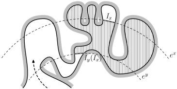
Figure 5: This figure shows an example of the last arc $I^{y}(I^{x})$ that a path to $I^{x}$ has to intersect ($I^{y}(I^{x})$ and $I^{x}$ are the gray lines) and the corresponding topological quadrilateral (the region shaded with vertical lines).

By $Q(I^{x})$ we denote the topological quadrilateral which is cut from $\Omega$ by the arcs $I^{x}$ and $I^{0}(I^{x})$. Denote

$$\ell\left(I^{x}\right)=\ell_{0}^{x}\left(I^{x}\right):=\int_{0}^{x}\frac{1}{\left|I^{y}(I^{x})\right|}dy.$$

By the second integral estimate of Lemma 2.13,

$$m(Q(I^{x}))\geq\ell\left(I^{x}\right).$$ (25)

Note that if $\gamma$ crosses $A$ and intersects $I^{x}$, then it makes an unforced crossing of $Q(I^{x})$, so we conclude that by Condition C3 the probability of crossing $A$ and intersecting $I^{x}$ is majorated by

$$K\,\exp\left(-\epsilon\ell\left(I^{x}\right)\right).$$ (26)

Denote also $\left|{\cal I}^{x}\right|:=\sum\left|I^{x}\right|$ and $\ell\left({\cal I}^{x}\right):=\int_{0}^{x}\frac{1}{\left|{\cal I}^{y}\right|}dy$

We call a collection of arcs $\left\{I_{j}\right\}$ (possibly corresponding to different $x$’s) separating, if every unforced crossing $\gamma$ intersects one of those. To deduce Condition G2, by (26) it is enough to find a separating collection of arcs such that

$$\sum_{j}\exp\left(-\epsilon\,\ell\left(I_{j}\right)\right)<\frac{1}{2K}.$$ (27)

Note that for every $x$ the total length $\left|{\cal I}^{x}\right|\leq 2\pi$, and so by our choice of constant $C$ we have

$$\ell\left({\cal I}^{\log C}\right)\geq\frac{\log C}{2\pi}\geq\frac{2}{\epsilon},$$

as well as

$$\exp\left(2-\epsilon\ell\left({\cal I}^{\log C}\right)\right)\leq\exp\left(2-\epsilon\frac{\log C}{2\pi}\right)\leq\exp\left(2-\log\left(2Ke^{2}\right)\right)=\frac{1}{2K}.$$

Therefore it is enough to establish that for any $w\in[0,\log C]$ with $\ell\left({\cal I}^{w}\right)\geq\frac{2}{\epsilon}$ there exist arcs $I_{j}$ separating ${\cal I}^{w}$ with the following estimate:

$$\sum_{j}\exp\left(-\epsilon\,\ell\left(I_{j}\right)\right)\leq\exp\left(2-\epsilon\ell\left({\cal I}^{w}\right)\right).$$ (28)

We will do this in an abstract setting for families of arcs. Besides properties mentioned above, we note that for any two arcs $I$ and $J$ the arcs $I^{x}(I)$ and $I^{x}(J)$ either coincide or are disjoint. Also without loss of generality any arc $I$ we consider satisfies $I\prec J$ for some $J\in{\cal I}^{w}$.

By a limiting argument it is enough to prove (28) for ${\cal I}^{w}$ of finite cardinality $n$, and we will do this by induction in $n$.

If $n=1$, then we take the only arc $J$ in ${\cal I}^{w}$ as the separating one, and the estimate (28) readily follows:

$$\exp\left(-\epsilon\,\ell\left(J\right)\right)=\exp\left(-\epsilon\,\ell\left({\cal I}^{w}\right)\right)<\exp\left(2-\epsilon\,\ell\left({\cal I}^{w}\right)\right).$$

Suppose $n>1$. Denote by $v$ the minimal number such that ${\cal I}^{v}$ contains more than one arc.

If

$$\ell_{v}^{w}\left({\cal I}^{w}\right):=\int_{v}^{w}\frac{1}{\left|{\cal I}^{y}\right|}dy<\frac{2}{\epsilon},$$

then we take the only arc $J$ in ${\cal I}^{v-\delta}$ as the separating one. The required estimate (28) then holds if $\delta$ is small enough:

$$\exp\left(-\epsilon\,\ell\left(J\right)\right) =\exp\left(-\epsilon\,\ell_{0}^{w}\left({\cal I}\right)+\epsilon\,\ell_{v-\delta}^{w}\left({\cal I}\right)\right)$$

$$\leq\exp\left(-\epsilon\,\ell\left({\cal I}_{0}^{w}\right)+\epsilon\frac{2}{\epsilon}\right)=\exp\left(-\epsilon\,\ell\left({\cal I}\right)+2\right).$$

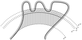
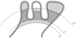
Figure 6: In this figure, the shading with diagonal lines represents the integral $\ell_{v}^{w}\left({\cal I}^{w}\right)$ which in the subfigure 6 is small and in 6 is big. In the first case the arc of the circle of radius $e^{v-\delta}$ gives the arc with desired properties. In the second case we use the induction hypothesis to find a set of arcs of circles with radii in the range $[e^{v},e^{w}]$. These arcs are here illustrated by gray lines and one of the topological quadrilaterals cut by an arc are illustrated in both subfigures by vertical shading.

Now assume that, on the contrary,

$$\ell_{v}^{w}\left({\cal I}^{w}\right)\geq\frac{2}{\epsilon}.$$

Suppose ${\cal I}^{v}$ is composed of the arcs $J_{k}$. For each $k$ denote by ${\cal I}_{k}^{x}$ the collection of arcs $I\in{\cal I}^{x}$ such that $J_{k}\prec I$. Since

$$\ell_{v}^{w}\left({\cal I}_{k}^{w}\right)\geq\ell_{v}^{w}\left({\cal I}^{w}\right)\geq\frac{2}{\epsilon},$$ (29)

we can apply the induction assumption to each of those collections ${\cal I}_{k}^{w}$ on the interval $x\in[v,w]$, obtaining a set of separating arcs $\left\{I_{j,k}\right\}_{j}$ such that

$$\sum_{j}\exp\left(-\epsilon\,\ell_{v}\left(I_{j,k}\right)\right)\leq\exp\left(2-\epsilon\ell_{v}^{w}\left({\cal I}_{k}\right)\right).$$ (30)

Then the desired estimate follows from

$$\sum_{j,k}\exp\left(-\epsilon\,\ell\left(I_{j,k}\right)\right)\leq \exp\left(-\epsilon\,\ell_{0}^{v}\left({\cal I}^{v}\right)\right)\leavevmode\nobreak\ \sum_{k}\sum_{j}\exp\left(-\epsilon\,\ell_{v}\left(I_{j,k}\right)\right)$$

$$\leq \exp\left(-\epsilon\,\ell_{0}^{v}\left({\cal I}^{v}\right)\right)\leavevmode\nobreak\ \sum_{k}\exp\left(2-\epsilon\ell_{v}^{w}\left({\cal I}_{k}^{w}\right)\right)$$

$$\overset{*}{\leq} \exp\left(-\epsilon\,\ell_{0}^{v}\left({\cal I}^{v}\right)\right)\leavevmode\nobreak\ \exp\left(2-\epsilon\ell_{v}^{w}\left({\cal I}^{w}\right)\right)$$ (31)

$$= \exp\left(2-\epsilon\ell\left({\cal I}^{w}\right)\right),$$

assuming we have the inequality (31$*$) above. To prove it we first observe that for $x\in[v,w]$,

$$\sum_{k}\left|{\cal I}_{k}^{x}\right|=\left|{\cal I}^{x}\right|.$$

Using Jensen’s inequality for the probability measure

$$\frac{dy}{\left|{\cal I}^{y}\right|\ell_{v}^{w}\left({\cal I}\right)},$$

and the convex function $x^{-1}$, we write

$$\ell_{v}^{w}\left({\cal I}_{k}\right) =\int_{v}^{w}\frac{1}{\left|{\cal I}_{k}^{y}\right|}dy=\int_{v}^{w}\left(\frac{\left|{\cal I}_{k}^{y}\right|}{\left|{\cal I}^{y}\right|\ell_{v}^{w}\left({\cal I}\right)}\right)^{-1}\frac{dy}{\left|{\cal I}^{y}\right|\ell_{v}^{w}\left({\cal I}\right)}$$

$$\geq\left(\int_{v}^{w}\frac{\left|{\cal I}_{k}^{y}\right|}{\left|{\cal I}^{y}\right|\ell_{v}^{w}\left({\cal I}\right)}\frac{dy}{\left|{\cal I}^{y}\right|\ell_{v}^{w}\left({\cal I}\right)}\right)^{-1}=\left(\int_{v}^{w}\frac{\left|{\cal I}_{k}^{y}\right|dy}{\left|{\cal I}^{y}\right|^{2}\ell_{v}^{w}\left({\cal I}\right)^{2}}\right)^{-1}.$$

Thus

$$\sum_{k}\frac{1}{\ell_{v}^{w}\left({\cal I}_{k}\right)} \leq\sum_{k}\left(\int_{v}^{w}\frac{\left|{\cal I}_{k}^{y}\right|dy}{\left|{\cal I}^{y}\right|^{2}\ell_{v}^{w}\left({\cal I}\right)^{2}}\right)={\int_{v}^{w}\frac{\sum_{k}\left|{\cal I}_{k}^{y}\right|dy}{\left|{\cal I}^{y}\right|^{2}\ell_{v}^{w}\left({\cal I}\right)^{2}}}$$

$$={\int_{v}^{w}\frac{dy}{\left|{\cal I}^{y}\right|}\,\frac{1}{\ell_{v}^{w}\left({\cal I}\right)^{2}}}={\ell_{v}^{w}\left({\cal I}\right)\frac{1}{\ell_{v}^{w}\left({\cal I}\right)^{2}}}=\frac{1}{\ell_{v}^{w}\left({\cal I}\right)}.$$ (32)

An easy differentiation shows that the function $F(x):=\exp\left(-\epsilon/x\right)$ vanishes at $0$, is increasing and convex on the interval $[0,\epsilon/2]$, and so is sublinear there. Observing that the numbers $1/\ell_{v}^{w}\left({\cal I}_{k}\right)$ as well as their sum belong to this interval by (29) and (32), we can write

$$\sum_{k}\exp\left(-\epsilon\ell_{v}^{w}\left({\cal I}_{k}\right)\right) =\sum_{k}F\left(1/\ell_{v}^{w}\left({\cal I}_{k}\right)\right)\leq F\left(\sum_{k}1/\ell_{v}^{w}\left({\cal I}_{k}\right)\right)$$

$$\leq F\left(1/\ell_{v}^{w}\left({\cal I}\right)\right)=\exp\left(-\epsilon\ell_{v}^{w}\left({\cal I}\right)\right),$$

thus proving the inequality (31$*$) and the desired implication.

This completes the circle of implications, thus proving Proposition 2.6.

3 Proof of the main theorem

In this section, we present the proof of Theorem 1.5. As a general strategy, we find an increasing sequence of events $E_{n}\subset X_{\mathrm{simple}}(\mathbb{D})$ such that

$$\lim_{n\to\infty}\inf_{\mathbb{P}\in\Sigma_{\mathbb{D}}}\mathbb{P}(E_{n})=1$$

and the curves in $E_{n}$ have some good properties which among other things guarantee that the closure of $E_{n}$ is contained in the class of Loewner chains.

The structure of this section is as follows. To use the main lemma (Lemma A.5 in appendix, which constructs the Loewner chain) we need to verify its three assumptions. In Section 3.2, it is shown that with high probability the curves will have parametrizations with uniform modulus of continuity. Similarly the results in Section 3.3 guarantee that the driving processes in the capacity parametrization have uniform modulus of continuity with high probability. In Section 3.4, a uniform result on the visibility of the tip $\gamma(t)$ is proven giving the uniform modulus of continuity of the functions $F$ of Lemma A.5. Finally in the end of this section we prove the main theorem and its corollaries.

A tool which makes many of the proofs easier is the fact that we can use always the most suitable form of the equivalent conditions. Especially, by the results of Section 2.2 if Condition G2 can be verified in the original domain then Condition G2 (or any equivalent condition) holds in any reference domain where we choose to map the random curve as long as the map is conformal. Furthermore, Condition G2 holds after we observe the curve up to a fixed time or a random time and then erase the observed initial part by conformally mapping the complement back to reference domain.

3.1 Reformulation of the main theorem

In this section we reformulate the main result so that its proof amounts to verifying four (more or less) independent properties, which are slightly technical to formulate. The basic definitions are the following, see Sections 3.2, 3.3 and 3.4 for more details. Assume that $\rho_{n}$ is a decreasing sequence such that $\rho_{n}\searrow 0$ as $n\to\infty$, that $\alpha,\alpha^{\prime},T,R$ are positive numbers and that $\psi:[0,\infty)\to[0,\infty)$ is continuous and strictly increasing function with $\psi(0)=0$. Define the following random variables

$$N_{0} =\sup\{n\geq 2\,:\,\gamma\text{ intersects $\partial B(1,\rho_{n-1})$ after intersecting $\partial B(1,\rho_{n})$}\}$$ (33)

$$C_{1,\alpha} =\inf\left\{C>0\,:\,\begin{gathered}\gamma\text{ can be parametrized s.t.}\\ |\gamma(s)-\gamma(t)|\leq C|t-s|^{\alpha}\quad\forall(t,s)\in[0,1]^{2}\end{gathered}\right\}$$ (36)

$$C_{2,\alpha^{\prime},T} =\inf\left\{C>0\,:\,\begin{gathered}|W_{\gamma}(s)-W_{\gamma}(t)|\leq C|t-s|^{\alpha^{\prime}}\quad\forall(t,s)\in[0,T]^{2}\end{gathered}\right\}$$ (38)

$$C_{3,\psi,T,R} =\inf\left\{C>0\,:\,\begin{gathered}|F_{\gamma}(t,y)-\hat{\gamma}(t)|\leq C\psi(y)\quad\forall(t,y)\in[0,T]\times[0,R]\end{gathered}\right\}$$ (40)

where $\hat{\gamma}=\Phi(\gamma)$ and

$$F_{\gamma}(t,y)=g_{t}^{-1}(W_{\gamma}(t)+i\,y)$$ (41)

which can be called a hyperbolic geodesic ending to the tip of the curve.

We will prove the next proposition in Sections 3.2, 3.3 and 3.4. Theorem 1.5 follows from the proposition (including the results of the next three subsections) and Lemma A.5.

Proposition 3.1.

If $\Sigma$ satisfies Condition G2 and $\Sigma_{\mathbb{D}}$ is as in (7), then the following statements hold

• The random curves $\gamma$, whose laws form the collection $\Sigma_{\mathbb{D}}$, are transient uniformly in the following sense: there exists a sequence $\rho_{n}$ such that the random variable $N_{0}$ is tight in $\Sigma_{\mathbb{D}}$.

• The family of measures $\Sigma_{\mathbb{D}}$ is tight in $X$: There exists $\alpha>0$ such that $C_{1,\alpha}$ is a tight random variable in $\Sigma_{\mathbb{D}}$.

• The family of measures $\Sigma_{\mathbb{D}}$ is tight in the sense of driving process convergence: There exists $\alpha^{\prime}>0$ such that $C_{2,\alpha^{\prime},T}$ is a tight random variable in $\Sigma_{\mathbb{D}}$ for each $T>0$.

• There exists $\psi$ such that $C_{3,\psi,T,R}$ is a tight random variable in $\Sigma_{\mathbb{D}}$ for each $T>0$, $R>0$.

3.2 Extracting weakly convergent subsequences of probability measures on curves

In this subsection, we first review the results of [2] and then we verify their assumption (which they call hypothesis H1) given that Condition G2 holds. At some point in the course of the proof, we observe that it is nicer to work with a smooth domain such as $\mathbb{D}$, hence justifying the effort needed to prove the equivalence of the conditions.

Aizenman and Burchard [2] made the following assumption on a collection of probability measures on the space of curves. They called it Hypothesis H1 and for us it is Condition G4.

Condition G4.

A collection of measures $\Sigma_{0}$ on $X(\mathbb{C})$ is said to satisfy a power-law bound on multiple crossings if for each $n$, there are constants $\Delta_{n}\geq 0$, $K_{n}>0$ such that

$$\mathbb{P}\big{(}\gamma\textrm{ makes $n$ crossings of }A(z_{0},r,R)\big{)}\leq K_{n}\left(\frac{r}{R}\right)^{\Delta_{n}}$$ (42)

for any annulus $A(z_{0},r,R)$ and for each $\mathbb{P}\in\Sigma_{0}$ and that satisfy $\Delta_{n}\to\infty$ as $n\to\infty$.

Remark 3.2.

The sequence $(\Delta_{n})$ can trivially be chosen to be non-decreasing. Hence it is actually enough to check that $\Delta_{n_{j}}\to\infty$ along a subsequence $n_{j}\to\infty$.

Based on this assumption Aizenman and Burchard proved the following result, see Theorem 1.1 and Theorem 2.3 in [2].

Theorem 3.3 (Aizenman–Burchard [2]).

Assume that a collection of measures $\Sigma_{0}$ on $X(\mathbb{C})$ satisfies Condition G4 and that $\gamma$ is uniformly bounded, i.e., there exists $R>0$ such that $\mathbb{P}(\gamma\subset B(0,R))=1$ for all $\mathbb{P}\in\Sigma_{0}$ Then the following statements hold.

1. The family of $\Sigma_{0}$ is tight and hence any sequence in $\Sigma_{0}$ contains a weakly convergent subsequence.

2. There exists exponents $\alpha>0$ and $\beta>0$ such that following random variables are tight on $\Sigma_{0}$

   $$Z_{\alpha}(\gamma) =\sup\big{\{}M(\gamma,l)\cdot l^{\alpha}\;:\;0<l<1\big{\}}$$ (43)

   $$\hat{Z}_{\beta}(\gamma) =\inf_{\hat{\gamma}}\,\sup\,\big{\{}w(\hat{\gamma},\delta)\cdot\delta^{-\beta}\;:\;0<\delta<1\big{\}}$$ (44)

   where we use the following definitions. The random variable $M(\gamma,l)$ is the minimum of the numbers $n$ such that there exists a partition $0=t_{0}<t_{1}<\ldots<t_{n}=1$ of the time interval $[0,1]$ such that $\operatorname{diam}(\gamma[t_{k-1},t_{k}])\leq l$ for any $k=1,2,\ldots,n$. The random variable $w(\hat{\gamma},\delta)$ is the modulus of continuity of the parametrization $\hat{\gamma}$ of $\gamma$, that is,

   $$w(\hat{\gamma},\delta)=\max\{\,|\hat{\gamma}(t)-\hat{\gamma}(s)|\;:\;(s,t)\in[0,1]^{2}\textrm{ s.t. }|s-t|\leq\delta\}.$$ (45)

   The infimum in $\hat{Z}_{\beta}(\gamma)$ is over all parametrizations $\hat{\gamma}$ of $\gamma$.

Remark 3.4.

A bound of the type $Z_{\alpha}(\gamma)\leq K$ for some $K>0$ and $\alpha>0$ was called tortuosity bound in [2] and similarly bound for $Z_{\beta}(\gamma)\leq K$ for some $K>0$ and $\beta>0$ is modulus of continuity bound. Existence of one type of bound implies existence of the other bound, which might hint how Condition G4 is sufficient assumption for this result.

Remark 3.5.

The compact subsets $K\subset X$ were characterized in Lemma 4.1 in [2]. A closed set $K\subset X$ is compact if and only if there exists a function $\psi:(0,1]\to(0,1]$ such that

$$M(\gamma,l)\leq\frac{1}{\psi(l)}$$

for any $\gamma\in K$ and for any $0<l\leq 1$. And this is equivalent to the existence of parametrization which allows a uniform bound on the modulus of continuity.

We will use the remainder of this section to show that Condition G3 implies Condition G4 and hence the results of Theorem 3.3. Notice that we assume Condition G3 in the original domain while Condition G4 is shown to hold in a smooth and bounded reference domain which we choose to be $\mathbb{D}$.

Proposition 3.6.

If $\Sigma$ satisfies Condition G3, then $\Sigma_{\mathbb{D}}$ satisfies Condition G4. Hence then also the conclusions of Theorem 3.3 hold.

Let $D_{t}=\mathbb{D}\setminus\gamma(0,t]$. Let $\tilde{C}>1$. For an annulus $A=A(z_{0},r,\tilde{C}^{3}r)$ define three concentric subannuli $A_{k}=A(z_{0},\tilde{C}^{k-1}r,\tilde{C}^{k}r)$, $k=1,2,3$. Define the index $I(A,D_{t})\in\{0,1,2,\ldots\}$ of $\gamma$ at time $t$ with respect to $A$ to be the minimal number of crossings of $A_{2}$ made by $\tilde{\gamma}$ where $\tilde{\gamma}$ runs over the set of all possible futures of $\gamma[0,t]$

$$\{\tilde{\gamma}\in X_{\mathrm{simple}}(D_{t})\,:\,\tilde{\gamma}\textrm{ connects }\gamma(t)\textrm{ to }b\}.$$

Consider a sequence of stopping times $\tau_{0}=0$ and

$$\tau_{k+1}=\inf\{t>\tau_{k}:\gamma[\tau_{k},t]\textrm{ crosses }A\}$$

where $k=0,1,2,\ldots$ Define also $\sigma_{0}=0$ and

$$\sigma_{k+1}=\inf\{t>\sigma_{k}:\gamma[\sigma_{k},t]\textrm{ crosses }A_{2}\}.$$

Since $\gamma(\tau_{k})$ and $\gamma(\tau_{k+1})$ lie in the different components of $\mathbb{C}\setminus A$, the curve $\gamma[\tau_{k},\tau_{k+1}]$ has to cross $A_{2}$ an odd number of times. Hence there are odd number of $l$ such that $\tau_{k}<\sigma_{l+1}<\tau_{k+1}$. For each $l$, $\gamma[\sigma_{l},\sigma_{l+1}]$ crosses $A_{2}$ exactly once and therefore the index changes by $\pm 1$. From this it follows that

$$I(A,D_{\tau_{k+1}})=I(A,D_{\tau_{k}})+2n-1$$

with $n\in\mathbb{Z}$.

Lemma 3.7.

Let $A=A(z_{0},r,R)$ be an annulus and let $A_{k},k=1,2,3$ be its subannuli as above.

1. If $A$ is not on $\partial\mathbb{D}$, i.e. $\overline{B(z_{0},r)}\cap\partial\mathbb{D}=\emptyset$, then on the event $\tau<1$, $I(A,D_{\tau})=1$, where $\tau$ is the hitting time of $\overline{B(z_{0},r)}$.

2. If $A$ is on $\partial D_{s}$, i.e. $\overline{B(z_{0},r)}\cap\partial D_{s}\neq\emptyset$, and the index increases from $I$ to $I+2n-1$, $n\geq 1$, during a minimal crossing $\gamma[s,t]$ of $A$ then the total number of unforced crossings of the annuli $A_{k}$, $k=1,2,3$, made by $\gamma[s,t]$ has to be at least $2n-1$.

Proof.

The statement (i) can be easily verified since the point $+1$ can be reached from $\gamma(\tau)$ in $D_{s}$ while making only one crossing by following a path close to the boundary of $D_{s}$.

Suppose now that $A$ is on $\partial D_{s}$. Let $m\leq m^{\prime}$ be such that

$$\sigma_{m-1}<s<\sigma_{m}\textrm{ and }\sigma_{m^{\prime}}<t<\sigma_{m^{\prime}+1}.$$

As we observed above if we set $y_{l}\mathrel{\mathop{:}}=I(A,D_{\sigma_{l}})-I(A,D_{\sigma_{l-1}})$ then these changes in the index take values $y_{l}\in\{-1,1\}$ and they sum up to

$$\sum_{l=m}^{m^{\prime}}y_{l}=2n-1,$$

that is, to the total change of the index during $[s,t]$.

We claim that the following two statements hold:

• If $y_{m^{\prime}}=1$ then the last crossing $\gamma[\sigma_{m^{\prime}},t]$ of a component of $A_{1}$ or $A_{3}$ has to be unforced as observed at time $\sigma_{m^{\prime}}$.

• If $y_{l}=1=y_{l+1}$ then the latter crossing $\gamma[\sigma_{l},\sigma_{l+1}]$ is an unforced crossing of $A_{2}$ as observed at time $\sigma_{l}$.

To prove these claims, let $h=m^{\prime}$ or $h=l$ (depending on the claim, respectively) and suppose that $y_{h}=1$. Let $C_{0}\subset\partial A_{2}\cap D_{\sigma_{h}}$ be the boundary arc of $A_{2}$ which has the property that any curve from $\gamma(\sigma_{h})$ to $+1$ in $D_{\sigma_{h}}$ has to intersect $C_{0}$ and $C_{0}$ is not separated from $\gamma(\sigma_{h})$ by any other such arc. Let $V_{0}$ be the component of $D_{\sigma_{h}}\setminus C_{0}$ which contains (a neighborhood of) $+1$ and let $V_{1}$ to be the component of $A_{2}\cap D_{\sigma_{h}}$ which has $\gamma(\sigma_{h})$ and $C_{0}$ on its boundary. See Figure 7. Then $\gamma(\sigma_{h})$ can be connected to $+1$ in $V_{0}\cup C_{0}\cup V_{1}$. Because we assumed that $y_{k}=1$, $\gamma(\sigma_{h})$ and $C_{0}$ are in the different circular boundary arcs of the annulus $A_{2}$ and thus it is clear that if $V_{1}\subset A_{2}$ was crossed next, then the index would decrease by one. Hence the next crossing in both of the scenarios has to be in the complement of $V_{0}\cup C_{0}\cup V_{1}$. Since $\gamma(\sigma_{h})$ can be connected to $+1$ in $V_{0}\cup C_{0}\cup V_{1}$, this crossing is unforced as observed at time $\sigma_{h}$. Thus the claims hold.

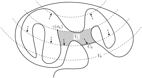
Figure 7: A sector of three concentric annuli with an initial segment of the interface. The boundaries of the annuli are the dashed circular arcs (which are only partly shown in the figure). If the index increases between times $\sigma_{h-1}$ and $\sigma_{h}$, then $\gamma(\sigma_{h})$ and $C_{0}$ are in different circular arcs . If the next crossing was in $V_{1}$, it would decrease the index. Hence in the scenarios in the proof of Lemma 3.7, the crossings corresponding to arrows on grey background are not allowed. Therefore a crossing which corresponds to one of the arrows on white background is going to happen next and those crossings are unforced.

The rest of the proof is divided in two cases depending on $y_{m^{\prime}}\in\{-1,1\}$. If $y_{m^{\prime}}=-1$, then

$$\max_{j=m,\ldots,m^{\prime}}\sum_{l=m}^{j}y_{l}\geq 2n.$$

Therefore there has to be at least $2n-1$ pairs $(l,l+1)$ so that $y_{l}=1=y_{l+1}$. This can be easily proven by induction. Hence the statement (ii) holds in this case by the second property we proved above.

If $y_{m^{\prime}}=1$, then there are at least $2n-2$ pairs $(l,l+1)$ so that $y_{l}=1=y_{l+1}$ by the same argument as in the previous case. In addition to this the last crossing $\gamma[\sigma_{m^{\prime}},t]$ is unforced crossing of $A_{1}$ or $A_{3}$ by the first property we proved above. Hence the statement (ii) holds also in this case. ∎

Now we are ready to give the proof of the main result of this section. Notice that here we need that the domain is smooth otherwise the number $n_{0}$ below wouldn’t be bounded. There are of course many ways to bypass this: for instance, if we want the measures to be supported on Hölder curves (including the end points on the boundary), then we need to assume that minimal number of crossings of annuli $A(z_{0},r,R)$ centered at $z_{0}=a$ or $z_{0}=b$ grows at most as a power of $r$ as $r\to 0$.

Proof of Proposition 3.6.

We will prove the first claim that if $\Sigma$ satisfies Condition G3, then $\Sigma_{\mathbb{D}}$ satisfies Condition G4. The rest of the proposition follows then from the results of [2] which we formulated above in Theorem 3.3.

First of all, we can concentrate on the case that the variables $z_{0},r,R$ are bounded. We can assume that $z_{0}\in B(0,3/2),r<1/2,R<1$. In the complementary case either the left-hand side of (42) is zero by the fact that there are no crossing of the annulus that stay inside the unit disc or the ratio $r/R$ is uniformly bounded away from zero. In the latter case the constant $K_{n}$ can be chosen so that the right-hand side of (42) is greater than one and (42) is satisfied trivially.

Denote as usual $A=A(z_{0},r,R)$. By the fact that $R<1$, at most one of the points $\pm 1$ is in $A$. If either $\pm 1$ is in $A$, denote the distance from that point to $z_{0}$ by $\rho$. Then $r<\rho<R$ and a trivial inequality shows that

$$\max\left\{\frac{\rho}{r},\frac{R}{\rho}\right\}\geq\sqrt{\frac{R}{r}}.$$

Hence for each annulus, it is possible to choose a smaller annulus inside it so that the points $\pm 1$ are away from that annulus and the ratio of the radii is still at least square root of the original one. If we are able to show existence of the constants $K_{n}$ and $\Delta_{n}$ for annuli $A$ such that $\{-1,1\}\cap A=\emptyset$ then constants $\hat{K}_{n}=K_{n}$ and $\hat{\Delta}_{n}=\Delta_{n}/2$ can be used for a general annulus.

Let $A$ be such that $\{-1,1\}\cap A=\emptyset$ and set $n_{0}$ and $\tau$ in the following way: if $\overline{B(z_{0},r)}$ intersects the boundary, let $n_{0}=1$ when $\overline{B(z_{0},r)}$ contains $-1$ or $1$ and $n_{0}=0$ otherwise and let $\tau=0$. If $\overline{B(z_{0},r)}$ doesn’t intersect the boundary, let $n_{0}=2$ and let $\tau=\inf\{t\in[0,1]\,:\,\gamma(t)\in\overline{B(z_{0},r)}\}$.

By Lemma 3.7, if there is a crossing of $A$ that increases the index, there are unforced crossings of the annuli $A_{k}$, $k=1,2,3$. We can apply this result after time $\tau$. If the curve doesn’t make any unforced crossings of the annuli $A_{k}$, $k=1,2,3$, then there are at most $n_{0}$ crossings of $A$. This argument generalizes so that if there are $n>n_{0}$ crossings of $A$, we apply Condition G3 $(n-n_{0})/2$ times in the annuli $A_{k}$, $k=1,2,3$, to get the bound

$$\mathbb{P}\left(\gamma\textrm{ makes $n$ crossings of }A(z_{0},r,R)\right)\leq K^{\frac{n-n_{0}}{2}}\,\cdot\,\left(\frac{r}{R}\right)^{\frac{\Delta}{6}(n-n_{0})}$$

for any $\mathbb{P}\in\Sigma_{\mathbb{D}}$. Hence the proposition holds for $\Delta_{n}=\Delta\cdot(n-2)/12$. ∎

3.3 Continuity of driving process and finite exponential moment

Let $\Phi:\mathbb{D}\to\mathbb{H}$ be a conformal mapping such that $\Phi(-1)=0$ and $\Phi(1)=\infty$. To make the choice unique, it is also possible to fix $\Phi(z)=\frac{2i}{1-z}+\mathcal{O}(1)$ as $z\to 1$, i.e.

$$\Phi(z)=i\frac{1+z}{1-z}.$$ (46)

Denote by $\Phi_{t}=\Phi\circ g_{t}$. We often shorten the notation by writing $\Phi\gamma=\Phi(\gamma)$.

Denote by $W(\,\cdot\,,\Phi\gamma)$ the driving process of $\Phi\gamma$ in the capacity parametrization. Our primary interest is to estimate the tails of the distribution of the increments of the driving process. Let’s first study what kind of events are those when $|W(t,\Phi\gamma)-W(s,\Phi\gamma)|$ is large. Suppose that $u$ and $L$ are positive real numbers such that $u/L$ is small. Consider a hull $K$ that is a subset of a rectangle $R_{L,u}=[-L,L]\times[0,u]$. If $K\cap[L,L+iu]\neq\emptyset$ then for any $z$ in this set, $0.9\,L\leq g_{K}(z)\leq 1.1\,L$ as proved below in Lemma A.11. On the other hand if $K\cap\,[-L+iu,L+iu]\neq\emptyset$ then $\mathrm{cap}_{\mathbb{H}}(K)\geq\frac{1}{4}u^{2}$. This is proved in Lemma A.13.

Based on this observation the following inequality holds

$$\mathbb{P}\left(\,\left|W\left(\frac{1}{4}u^{2},\Phi\gamma\right)\right|\geq 2L\,\right)\leq\mathbb{P}\big{(}\,\operatorname{Re}[(\Phi\gamma)(\tau_{R_{L,u}})]=\pm L\,\big{)},$$ (47)

where $\tau_{R_{L,u}}=\inf\{\,t\in[0,1]\;:\;\Phi\gamma(t)\in\mathbb{H}\cap\partial R_{L,u}\,\}$. Therefore we study the event that the curve exits a rectangular neighborhood of the origin in the upper half-plane through the sides of the rectangle. Notice also that the capacity $t=u^{2}/4$ corresponds to the height $2\sqrt{t}=u$ of the rectangle in the inequality (47). This is ultimately the source for the exponent $\alpha<1/2$ and for the term $\sqrt{t}$ in (9) in the main theorem (Theorem 1.5). Figure 8 illustrates both this correspondence and the proof of the next proposition.

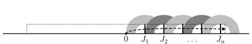
Figure 8: If $\sup\{|W_{u}-W_{s}|\;:\;u\in[s,t]\}\geq L$, then the curve $u\mapsto g_{s}(\gamma(u))-W_{s}$, $s\leq u\leq t$, exits the rectangle $[-L,L]\times[0,2\sqrt{t-s}]$ from one of the sides $\{\pm L\}\times[0,2\sqrt{t-s}]$. Especially the curve has to intersect all the vertical lines and make an unforced crossing of each of the annuli centered at the base points of those lines.

Proposition 3.8.

If Condition G2 holds, then there are constants $K>0$ and $c>0$ so that

$$\mathbb{P}\big{(}\,\operatorname{Re}[(\Phi\gamma)(\tau_{R_{L,u}})]=\pm L\,\big{)}\leq Ke^{-c\frac{L}{u}}$$ (48)

for any $0<u<L$.

Proof.

If Condition G2 holds then it also holds in $\mathbb{H}$ by the results of Section 2.2. Let $C>1$ be the constant of Condition G2 in $\mathbb{H}$.

By symmetry, it is enough to consider the event $E$ that $\Phi\gamma$ exits the rectangle $R_{L,u}$ from the right-hand side $\{L\}\times[0,u]$. Let $n=\lfloor L/(Cu)\rfloor$. Consider the lines $J_{k}=\{Cu\cdot k\}\times[0,u]$, $k=1,2,\ldots,n$. On the event $E$, each of the lines $J_{k}$ are hit before $\tau_{R_{L,u}}$ and the hitting times are ordered

$$0<\tau_{J_{1}}<\tau_{J_{2}}<\ldots<\tau_{J_{n}}\leq\tau_{R_{L,u}}<1$$

See Figure 8.

Let $x_{k}=Cu\cdot k$ which is the base point of $J_{k}$. On the event $E$ the annulus $A(x_{1},u,Cu)$ is crossed and after each $\tau_{J_{k}}$ the annulus $A(x_{k+1},u,Cu)$ is crossed. Hence Condition G2 can be applied with the stopping times $0,\tau_{J_{1}},\ldots,\tau_{J_{n-1}}$ and the annuli $A(x_{1},u,Cu)$, $A(x_{2},u,Cu),\ldots$, $A(x_{n},u,Cu)$. This gives the upper bound $2^{-n}$ for the probability of $E$. Hence the inequality (48) follows with suitable constants depending only on $C$. ∎

We can now apply the above bounds (47) and (48) to show the next proposition which can be interpreted in the following way. The first statement shows the uniform transience of the curves (uniform over $\mathbb{P}\in\Sigma_{\mathbb{D}}$) in the same sense as in Proposition 3.1. The second statement is a sufficient technical statement for the Hölder continuity of the driving processes and is used in the proof of Theorem 3.10. The third statement is needed for the exponential integrability of the driving process in Theorem 1.5.

Proposition 3.9.

Let $\upsilon(t)=\mathrm{cap}_{\mathbb{H}}(\Phi\gamma[0,t])/2$ for any $t\in[0,1)$ and define $\upsilon(1)=\lim_{t\to 1}\upsilon(t)\in(0,\infty]$. If Condition G2 holds, then

1. For all $\mathbb{P}\in\Sigma_{\mathbb{D}}$, $\mathbb{P}(\upsilon(1)=\infty)=1$. There exists a sequence $b_{n}\in\mathbb{R}$ such that

   $$\mathbb{P}\left(\sup_{0\leq t\leq n}|W_{t}(\hat{\gamma})|\leq b_{n}\right)\geq 1-\frac{1}{n}$$ (49)

   for any $\mathbb{P}\in\Sigma_{\mathbb{D}}$.

2. Fix $T>0$ and $0<\alpha<\frac{1}{2}$. Let $X^{\prime}\subset X_{\mathrm{simple}}(\mathbb{D})$ be the set of simple curves such that $\upsilon(1)>T$. Define

   $$G_{n}=\left\{\gamma\in X^{\prime}:\sup_{j2^{-n}\leq u\leq(j+1)2^{-n}}|W_{u}(\hat{\gamma})-W_{j2^{-n}}(\hat{\gamma})|\leq 2^{-\alpha n}\right\}.$$ (50)

   Then for large enough $n\geq n_{0}(\alpha,T,K,c)$

   $$\mathbb{P}\big{(}G_{n}\big{)}\geq 1-2^{-n}$$

   for any $\mathbb{P}\in\Sigma_{\mathbb{D}}$.

3. There exists constants $\varepsilon>0$ and $C>0$ such that

   $$\mathbb{E}_{\mathbb{P}}\left[\exp\left(\varepsilon\max_{s\in[0,t]}|W_{s}(\hat{\gamma})|/\sqrt{t}\right)\right]\leq C$$ (51)

   for any $t>0$ and for any $\mathbb{P}\in\Sigma_{\mathbb{D}}$. Here $\mathbb{E}_{\mathbb{P}}$ is the expected value with respect to $\mathbb{P}$.

Proof.

Notice first that in the inequality (47) we can replace $|W(u^{2}/4,\Phi\gamma)|$ on the left by $\max_{0\leq s\leq u^{2}/4}|W(u^{2}/4,\Phi\gamma)|$. This stronger version follows from the very same observation.

1. Let $b_{n}=(4/c)\,\sqrt{n}\log(K\,n)$. Then by (47) and (48)

$$\mathbb{P}\left(\sup_{0\leq t\leq n}|W_{t}(\hat{\gamma})|>b_{n}\right)\leq K\exp\left(-c\frac{b_{n}}{4\sqrt{n}}\right)=\frac{1}{n}.$$ (52)

In particular, $\mathbb{P}(\upsilon(1)=\infty)=1$.

2. Estimate the probability of the complement of $G_{n}$ by the following sum

$$\mathbb{P}\left(G_{n}^{c}\right) \leq\sum_{j=0}^{2^{n}}\mathbb{P}\left(\max_{u\in[T(j-1)2^{-n},Tj2^{-n}]}|W_{u}-W_{T(j-1)2^{-n}}|>2^{-\alpha n}\right)$$

$$\leq K2^{n}e^{-(c/4)T^{-1/2}2^{(1/2-\alpha)n}}\leq 2^{-n}$$

for $n$ large enough depending on $\alpha,T,K,c$.

3. Fix $t>0$ and denote the random variable $\max_{s\in[0,t]}|W_{s}(\hat{\gamma})|$ by $Z$. Let $\varepsilon>0$, which we fix in a moment, and $\phi(x)=\exp(\varepsilon x/\sqrt{t})$. Then by an equality following from Fubini’s theorem and by the bound (48)

$$\mathbb{E}_{\mathbb{P}}(\phi(Z)) =\phi(0)+\int_{0}^{\infty}\phi^{\prime}(x)\mathbb{P}(Z\geq x)\,\mathrm{d}x\leq 1+\frac{K\varepsilon}{\sqrt{t}}\int_{0}^{\infty}\exp\left(\left(\varepsilon-\frac{c}{4}\right)\frac{x}{\sqrt{t}}\right)\mathrm{d}x$$

$$=1+K\varepsilon\int_{0}^{\infty}\exp\left(\left(\varepsilon-\frac{c}{4}\right)y\right)\mathrm{d}y$$

where $K,c$ are as in (3.8). Choose $\varepsilon<\frac{c}{4}$. Then the constant on the right is finite. It is also independent of $t$ and $\mathbb{P}$ as claimed. ∎

Finally we reformulate the above somewhat technical results into the following cleaner theorem (implied by the previous proposition as explained above) on the Hölder continuity of the driving processes. The theorem follows from the statement 2 of Proposition 3.9 above and Lemma 7.1.6 and the proof of Theorem 7.1.5 in [14].

Theorem 3.10.

If Condition G2 holds, then for each $\mathbb{P}\in\Sigma_{\mathbb{D}}$ the curve $\gamma$ is a Loewner chain which has $\alpha$-Hölder continuous driving process $\mathbb{P}$-almost surely for any $0<\alpha<1/2$ and the $\alpha$-Hölder norm of the driving process restricted to $[0,T]$ for $T>0$ is stochastically bounded.

3.4 Continuity of the hyperbolic geodesic to the tip

In the proof of the main theorem, we are going to apply Lemma A.5 of the appendix. Therefore we repeat here the following definition: for a simple curve $\gamma$ in $\mathbb{H}$, let $(g_{t})_{t\in\mathbb{R}_{+}}$ and $(W(t))_{t\in\mathbb{R}_{+}}$ be its Loewner chain and driving function. Then we define the hyperbolic geodesic from $\infty$ to the tip $\gamma(t)$ as $F:\mathbb{R}_{+}\times\mathbb{R}_{+}\to\overline{\mathbb{H}}$ by

$$F(t,y)=g_{t}^{-1}(W(t)+i\,y).$$

The corresponding geodesic in $\mathbb{D}$ for the curve $\Phi^{-1}\gamma$ is

$$F_{\mathbb{D}}(t,y)=\Phi^{-1}\circ F(t,y).$$ (53)

Consider now the collection $\Sigma_{\mathbb{D}}$ and the random curve $\gamma$ in $X_{\mathrm{simple}}(\mathbb{D},-1,+1)$. Define $F$ and $F_{\mathbb{D}}$ as above for the curves $\Phi\gamma$ and $\gamma$, respectively. For $\rho>0$, let $\tau_{\rho}$ be the hitting time of $B(1,\rho)$, i.e., $\tau_{\rho}$ is the smallest $t$ such that $|\gamma(t)-1|\leq\rho$. The following is the main result of this subsection.

Theorem 3.11.

Suppose that $\Sigma$ satisfies Condition G2. There exists a continuous increasing function $\psi:\mathbb{R}_{+}\to\mathbb{R}_{+}$ such that $\psi(0)=0$ and for any $\rho>0$ and $\varepsilon>0$ there exists $\delta>0$ such that

$$\mathbb{P}\left(\begin{gathered}\sup_{t\in[0,\tau_{\rho}]}\left|F(t,y^{\prime})-F(t,y)\right|\leq\psi(|y-y^{\prime}|)\\ \forall y,y^{\prime}\in[0,L]\text{ s.t. }|y-y^{\prime}|\leq\delta\end{gathered}\right)\geq 1-\varepsilon$$ (54)

for each $\mathbb{P}\in\Sigma_{\mathbb{D}}$.

The proof is postponed after an auxiliary result, which is interesting in its own right. Namely, the next proposition gives a “superuniversal” arms exponent, i.e., the property is uniform for basically all models of statistical physics: under Condition G2 a certain event involving six crossings of an annulus has small probability to occur anywhere. Therefore the corresponding six arms exponent, if it exists, has value always greater than $2$. To see this, suppose that the probability of this six arms event in a single annulus $A(z_{0},r,R)$ tends to zero as $r^{\alpha}$ when $r\to 0$. Then we can sum over the lattice $r\mathbb{Z}^{2}$ and all annuli of the form $A(z,2r,R/4)$ where $z$ is a lattice point and get upper and lower bounds of the form $r^{\alpha-2}$ for seeing this six arms event in anywhere (in any annulus of the form $A(z_{0},r,R)$). Hence if this goes to zero, we must have $\alpha>2$.

Let $D_{t}=\mathbb{D}\setminus\gamma(0,t]$ and define the following event event $E(r,R)=E_{\rho}(r,R)$ on $X_{\mathrm{simple}}(\mathbb{D})$: Define $E(r,R)$ as the event that there exists $(s,t)\in[0,\tau]^{2}$ with $s<t$ such that

• $\operatorname{diam}\big{(}\,\gamma[s,t]\,\big{)}\geq R$ and

• there exists a crosscut $C$, $\operatorname{diam}(C)\leq r$, that separates $\gamma(s,t]$ from $B(1,\rho)$ in $\mathbb{D}\setminus\gamma(0,s]$.

Denote the set of such pairs $(s,t)$ by $\mathcal{T}(r,R)$.

Let’s first demonstrate that the event $E(r,R)$ implies a certain six arms event (four arms if it occurs near the boundary) occurring somewhere in $\mathbb{D}$ — the converse statement is also true, although we don’t need it here. If $C$ is as in the definition of $E(r,R)$, then for $r<\min\{\rho,R\}/2$ at least one of the end points of $C$ has to lie on $\gamma(0,s]$. Let $T(C)\leq s$ be the largest time such that $\gamma(T(C))\in\overline{C}$. Then also $(T(C),t)\in\mathcal{T}(r,R)$ and we easily see that $\gamma[T(C),t]$ makes a crossing of $(A(\gamma(T(C)),r,R/2))^{u}_{T(C)}$ and is therefore unforced. Moreover, $\gamma[0,T(C)]$ contains at least three crossings of $A(\gamma(T(C)),r,R/2)$, when $\gamma(T(C))$ is sufficiently far from the boundary, or one crossing, when $\gamma(T(C))$ is close to the boundary. Otherwise the above crossing couldn’t be unforced. See also Figure 3(a). Finally, after $t$ the curve $\gamma$ has to still make at least two crossings to reach the target point $+1$. Adding these numbers together, we conclude that on the event $E(r,R)$ there is $z_{0}\in\mathbb{D}$ such that $A(z_{0},r,R/2)$ contains at least six crossings when $|z_{0}|<1-r$ or four crossings when $|z_{0}|\geq 1-r$ and at least one of the crossings is unforced.

Now we know that $E(r,R)$ is a proper subevent of the full six arms event. By the next result its probability is small.

Proposition 3.12.

If $\Sigma_{\mathbb{D}}$ satisfies Condition G2, then as $r\to 0$

$$\sup\{\mathbb{P}\left(E(r,R)\right)\,:\,\mathbb{P}\in\Sigma_{\mathbb{D}}\}=o(1).$$

Remark 3.13.

Since $\mathbb{P}\left(E(r,R)\right)$ is decreasing in $R$, the bound is uniform for $R\geq R_{0}>0$.

The idea of the proof is the following: divide the curve $\gamma$ into $N$ arcs

$$J_{k}=\gamma[\sigma_{k-1},\sigma_{k}]$$ (55)

$0=\sigma_{0}<\sigma_{1}<\ldots<\sigma_{N}=1$ such that $\operatorname{diam}(J_{k})\leq R/4$, $k=1,2,\ldots,N$. Let $J_{0}=\partial\mathbb{D}$. For the event $E(r,R)$, firstly there has to exist a fjord of depth $R$ with a mouth formed by some pair $(J_{j},J_{k})$, $j<k$, and the number of such pairs is less than $N^{2}$. Secondly, there has to be a piece of the curve which enters the fjord, hence resulting in an unforced crossing. Hence (given $N^{2}$) the probability that $E(r,R)$ occurs is less than $const.\cdot N^{2}(r/R)^{\Delta}$.

Proof.

Suppose that $0<r<R/20$. We will specify more carefully in the end of the proof how small $r$ is for given $R$.

It is useful to do this by defining $\sigma_{k}$ as stopping times by setting $\sigma_{k}=0$, $k\leq 0$, and then recursively

$$\sigma_{k}=\sup\left\{t\in[\sigma_{k-1},1]:\operatorname{diam}\big{(}\gamma[\sigma_{k-1},t]\big{)}<\frac{R}{4}\right\}.$$

Let $J_{k}$, $k>0$, be as in (55) and let $J_{0}=\partial\mathbb{D}$. Observe that if the curve is divided into pieces that have diameter at most $R/4-\varepsilon$, $\varepsilon>0$, then none of these pieces can contain more than one of the $\gamma(\sigma_{k})$. Therefore $N\leq\inf_{\varepsilon>0}M(\gamma,R/4-\varepsilon)\leq M(\gamma,R/8)$ where $M$ is as in Theorem 3.3. By that theorem $N$ is stochastically bounded, which we will use below.

Define also stopping times

$$\tau_{j,k}=\inf\{\,t\in[\sigma_{k-1},\sigma_{k}]\;:\;\operatorname{dist}(\gamma(t),J_{j})\leq 2r\}.$$ (56)

for $0\leq j<k$. If the set is empty, let’s define the infimum to be equal to $1$.

Suppose that the event $E(r,R)$ occurs. Take a crosscut $C$ and a pair of times $0\leq s<t\leq 1$ as in the definition of $E(r,R)$.

Let $V\subset D_{s}$ be the connected component $D_{s}\setminus C$ which is disconnected from $+1$ by $C$ in $D_{s}$. Let $j<k$ be such that the end points of $C$ are on $J_{j}$ and $J_{k}$. Then it holds that the stopping time $\tau\mathrel{\mathop{:}}=\tau_{j,k}<1$ and we can set $z_{1}=\gamma(\tau_{j,k})$. Let $z_{2}$ be any point on $J_{j}$ such that $|z_{1}-z_{2}|=2r$.

Let $C^{\prime}=[z_{1},z_{2}]\mathrel{\mathop{:}}=\{\lambda\,z_{1}+(1-\lambda)\,z_{2}\,:\,\lambda\in[0,1]\}$ and

$$V^{\prime}=\{z\in V\,:\,z\text{ is disconnected from $+1$ by $C^{\prime}$ in $D_{\tau}$}\}$$

and let $D^{\prime}=D_{s}\setminus V$.

We claim that the event of an unforced crossing of $(A(z_{1},2r,R/2))^{u}_{\tau}$ occurs.

To prove this, notice first that $\partial D^{\prime}=\partial\mathbb{D}\cup\gamma[0,t_{C}]\cup C$ where $t_{C}\in[0,1]$ is the unique time such that $\{\gamma(t_{C})\}=\overline{C}\cap J_{k}$, i.e., the point $\gamma(t_{C})$ is the end point of $C$ which lies on $J_{k}$. Therefore $\partial D^{\prime}\subset(\partial\mathbb{D}\cup\gamma[0,\tau])\cup(J_{k}\cup C)$. Hence $(J_{k}\cup C)$ separates the set $V$ from $+1$ in $D_{\tau}$. Since $V\setminus V^{\prime}$ is separated from $V^{\prime}$ by $C^{\prime}$ in $D_{\tau}$, we see that $V\setminus V^{\prime}$ is a subset of the union of the bounded components of $\mathbb{C}\setminus(J_{j}\cup J_{k}\cup C\cup C^{\prime})$. Consequently $V\setminus V^{\prime}\subset B(z_{1},R/4+3r)$.

Now since we known that $V\setminus V^{\prime}\subset B(z_{1},R/4+3r)$, $\gamma[s,t]\subset V$ and $\gamma[s,t]$ is connected, we can find $[s^{\prime},t^{\prime}]\subset(\tau,t]$ such that $\gamma[s^{\prime},t^{\prime}]$ is a subset of $\overline{V^{\prime}}$ and it crosses $A(z_{1},2r,R/2)$. Hence we have shown that $\gamma[s,t]$ contains an unforced crossing of $A_{j,k}\mathrel{\mathop{:}}=A(z_{1},2r,R/2)$ as observed at time $\tau=\tau_{j,k}$. Consequently if we define $E_{j,k}=E_{j,k}(r,R)$ as

$$E_{j,k}=\left\{\gamma\in X_{\mathrm{simple}}(\mathbb{D},-1,+1)\,:\,\begin{gathered}\gamma[\tau_{j,k},1]\text{ contains a crossing of }A_{j,k}\\ \text{which is contained in }(A_{j,k})^{u}_{\tau_{j,k}}\end{gathered}\right\}$$ (57)

we have shown that $E(r,R)\subset\bigcup_{j=0}^{\infty}\,\bigcup_{k=j+1}^{\infty}\,E_{j,k}$.

Let $\varepsilon>0$ and choose $m\in\mathbb{N}$ such that $\mathbb{P}(N>m)\leq\varepsilon/2$ for all $\mathbb{P}\in\Sigma_{\mathbb{D}}$. Now

$$\mathbb{P}(E(r,R))\leq \mathbb{P}(N>m)+\mathbb{P}\left[\;\bigcup_{0\leq j<k}\{N\leq m\}\cap E_{j,k}\right]$$

$$\leq \frac{\varepsilon}{2}+\mathbb{P}\left[\;\bigcup_{0\leq j<k\leq m}\{N\leq m\}\cap E_{j,k}\right]$$

$$\leq \frac{\varepsilon}{2}+\sum_{0\leq j<k\leq m}\mathbb{P}\left[\{N\leq m\}\cap E_{j,k}\right]$$

$$\leq \frac{\varepsilon}{2}+Km^{2}\left(\frac{r}{R}\right)^{\Delta}\leq\varepsilon$$ (58)

when $r$ is smaller than $r_{0}>0$ which depends on $R$ and $\varepsilon$. Here we used the facts that $\{N\leq m\}\cap E_{j,k}=\emptyset$ when $k>m$ and that $\mathbb{P}[\{N\leq m\}\cap E_{j,k}]\leq\mathbb{P}[E_{j,k}]$. ∎

Proof of Theorem 3.11.

In this proof, we work on the unit disc. Fix $\rho>0$ and let $\tau=\tau_{\rho}$ as above. Let $D^{\prime}=\mathbb{D}\setminus\overline{B(1,\rho)}$. Since $\Phi$ and $\Phi^{-1}$ are uniformly continuous on $D^{\prime}$ and $\Phi(D^{\prime})$, respectively, it is sufficient to prove the corresponding claim for $F_{\mathbb{D}}$. Furthermore it is sufficient to show that $|F_{\mathbb{D}}(t,y)-\gamma(t)|\leq\psi(y)$ for $0<y\leq\delta$, because $y\mapsto F_{\mathbb{D}}(t,y)$, $y\in[\delta,1]$, is equicontinuous family by Koebe distortion theorem.

Let $R_{n}>0$, $n\in\mathbb{N}$, be any sequence such that $R_{n}\searrow 0$ as $n\to\infty$. By the previous proposition, we can choose a sequence $r_{n}$, $n\in\mathbb{N}$, such that $r_{n}<R_{n}$ and

$$\mathbb{P}(E(r_{n},R_{n}))\leq 2^{-n}$$ (59)

for all $n\in\mathbb{N}$ and for all $\mathbb{P}\in\Sigma_{\mathbb{D}}$. Therefore the random variable $N\mathrel{\mathop{:}}=\max\{n\in\mathbb{N}\,:\,\gamma\in E(r_{n},R_{n})\}$ is tight: for each $\varepsilon>0$ there exists $m\in\mathbb{N}$ such that

$$\mathbb{P}(N\leq m)\geq 1-\varepsilon$$ (60)

for all $\mathbb{P}\in\Sigma_{\mathbb{D}}$. Fix now $\varepsilon>0$ and let $m\in\mathbb{N}$ be such that (60) holds.

Define $n_{0}(\delta)$ to be the maximal integer such that the inequality

$$\frac{2\pi}{\sqrt{|\log\delta|}}\leq r_{n_{0}(\delta)}$$ (61)

holds. For given $0<\delta<1$, there is a $\delta^{\prime}\in[\delta,\delta^{1/2}]$ which can depend on $t$ and $\gamma$ such that the crosscut $C\mathrel{\mathop{:}}=\{\Phi^{-1}\circ g_{t}^{-1}(W(t)+i\delta^{\prime}e^{i\theta})\,:\,\theta\in(0,\pi)\}$ has length less than $2\pi/\sqrt{|\log\delta|}$, see Proposition 2.2 in [26].

Now if $N>n_{0}(\delta)$, then there must be a path from $w\mathrel{\mathop{:}}=\Phi^{-1}\circ g_{t}^{-1}(W(t)+i\delta^{\prime})$ to $\gamma(t)$ in $D_{t}$ that has diameter less than $R_{n_{0}(\delta)}$. By Gehring-Hayman theorem (Theorem 4.20 in [26]) the diameter of the hyperbolic geodesic $y\mapsto F_{\mathbb{D}}(t,y)$, $0\leq y\leq\delta^{\prime}$, is of the same order as the smallest possible diameter of the curve which connects $w$ with $\gamma(t)$ in $D_{t}$. Consequently there is a universal constant $c>0$ such that

$$\operatorname{diam}\{F_{\mathbb{D}}(t,y)\,:\,y\in[0,\delta]\}\leq cR_{n_{0}(\delta)}$$ (62)

for all $t\in[0,\tau]$, for all $\delta>0$ such that $n_{0}(\delta)>m$ and for all $\gamma$ such that $N\leq m$. ∎

3.5 Proof of the main theorem

Proof of Theorem 1.5 (Main theorem).

Fix $\varepsilon>0$. We will first choose four events $E_{k}$, $k=1,2,3,4$, that have large probability, namely,

$$\mathbb{P}(E_{k})\geq 1-\varepsilon/4$$ (63)

for all $\mathbb{P}\in\Sigma_{\mathbb{D}}$. Then those events have large probability occurring simultaneously since

$$\mathbb{P}\left(\,\bigcap_{k=1}^{4}E_{k}\,\right)\geq 1-\varepsilon.$$ (64)

Once we have defined $E_{k}$, denote $E=\bigcap_{k=1}^{4}E_{k}$.

We choose $E_{1}$ in such a way that the half-plane capacity of $\gamma[0,t]$ goes to infinity as $t\to\infty$ in a tight way on $\Sigma_{\mathbb{D}}$. We use Proposition 3.9 and choose $E_{1}$ the intersection of the events in the inequality (49) where $n=k^{2}$ runs from $k=m_{1}$ to $\infty$ where $m_{1}$ is chosen so that (63) holds. Then we choose $E_{2}$ and $E_{3}$ so that $E_{2}$ is the set of simple curves which are in some parametrization Hölder continuous with a Hölder exponent $\alpha_{c}>0$ and a Hölder constant $K_{c}$ and $E_{3}$ is the set of simple curves which have in the capacity parametrization Hölder continuous driving process with a Hölder exponent $\alpha_{d}>0$ and a finite Hölder norm $K_{d,T}$ for any $T>0$ when the process is restricted to the time interval $[0,T]$. (Here $K_{d,T}$ is naturally increasing in $T$.) Using Proposition 3.6 and Theorem 3.10 the constants are chosen so that the bound (63) is satisfied. Finally using Theorem 3.11 we set $E_{4}$ to be the set of simple curves that have function $\psi_{\rho}$ for each $\rho>0$ as in Theorem 3.11 and $\delta>0$ such that the geodesic to the tip is continuous with $|F(t,y)-F(t,y^{\prime})|\leq\psi_{\rho}(|y-y^{\prime}|)$ for $|y-y^{\prime}|<\delta$ and $t\in[0,\tau_{\rho}]$. Also here $\psi$ and $\delta>0$ are chosen so that (63) holds.

Now by Lemma A.5 of the appendix, the set $E$ is relatively compact in the convergence in the path convergence and in the driving convergence (and in the convergence of curves in the capacity parametrization) and the closure of $E$ is the same in both topologies as the following argument shows: for a sequence $\gamma_{n}\in E$ we can choose subsequence such that $\gamma_{n}$ converges in $X$ and $W_{n}$ converges uniformly on compact subsets of $[0,\infty)$ and $F_{n}$ converges uniformly on compact subsets of $[0,\infty)\times[0,\infty)$. Then by Lemma A.5, the limits agree in the sense that if we parametrize $\lim_{n\to\infty}\gamma_{n}$ by the capacity forms a Loewner chain that is driven by $\lim_{n\to\infty}\gamma_{n}$.

Since $E$ is precompact in the space of curves, we have shown that $\Sigma_{\mathbb{D}}$ is a tight family of probability measures on $X$, especially, and hence by Prohorov’s theorem we can choose for any sequence $\mathbb{P}_{n}\in\Sigma_{\mathbb{D}}$ a weakly convergent subsequence. This shows the first claim. The claims (i)–(v) of Theorem 1.5 follow from taking the closure of $E$ in any of the above topologies. Any subsequent weak limit $\mathbb{P}^{*}$ of $\mathbb{P}_{n}\in\Sigma_{\mathbb{D}}$ satisfies $\mathbb{P}^{*}(\overline{E})\geq\limsup_{n\to\infty}\mathbb{P}_{n}(\overline{E})\geq 1-\varepsilon$. Hence these claims holds $\mathbb{P}^{*}$ almost surely.

The last claim of Theorem 1.5 on the exponential integrability of the driving process follows similarly from the claim 3 of Proposition 3.9. ∎

3.6 The proofs of the corollaries of the main theorem

In this section we will prove Corollaries 1.7 and 1.8.

Proof of Corollary 1.7.

If $\gamma^{(n)}$ satisfy Condition G2 and its law is $\mathbb{P}_{n}$, then by (the proof of) Theorem 1.5 for each $\varepsilon>0$ we can choose an event $E$ satisfying $\inf_{n}\mathbb{P}_{n}(E)\geq 1-\varepsilon$ such that $E$ is relatively compact in all three topologies of the statement of Corollary 1.7. This fact follows from Lemma A.5 when for any sequence $\tilde{\gamma}_{n}\in E$ we pass to a subsequence where $\tilde{\gamma}_{n_{k}}$ converges in $X$, its driving term converges uniformly on compact intervals and the hyperbolic geodesic $F_{n}$ converges on compact sets. By Lemma A.5, we get the convergence in the capacity parametrization and, in addition, it holds that these limits agree in the sense that the limiting curve is driven by the limiting driving term. Since $E$ is relatively compact, the sequence $\mathbb{P}_{n}$ is tight in the same topology.

By this tightness, we see that if the sequence of random curves $\gamma^{(n)}$ or the sequence of driving processes $W^{(n)}$ converges in one of the three topologies, it converges also in the two other topologies. The argument for this is essentially the same as above. We pass to a subsequence where the convergence takes place also in the other topology. Then we notice that the sequence of the laws satisfies $\inf_{n}\mathbb{P}_{n}(E)\geq 1-\varepsilon$ hence the probability for the limiting objects to agree in the above sense is at least $1-\varepsilon$. Since this holds for any $\varepsilon$, the law of the other limiting object is uniquely determined. Therefore there is no need to pass to a subsequence, but the entire sequence converges. ∎

For the proof of Corollary 1.8 notice first that by the proof of C3$\Rightarrow$G2 in Section 2.2 we have constants $C_{1},C_{2}$ such that if $Q\subset U$ is a simply connected domain, whose boundary consists of a subset of $\partial U$ and some subsets of $U$ which are crosscuts $S_{0}$ and $S_{2}^{j}$, $j=1,2,\ldots$, (finite or infinite set), and if $Q$ has the property that it doesn’t disconnect $a$ from $b$ and $S_{0}$ is the “outermost” of the crosscuts (disconnecting the others from $a$ and $b$), then

$$\mathbb{P}(\gamma\text{ crosses }Q)\leq C_{1}\exp(-C_{2}m(Q))$$ (65)

where crossing means that $\gamma$ intersects one of the $S_{2}^{j}$’s and $m(Q)$ is the extremal length of the curve family connecting $S_{0}$ to $\bigcup_{j}S_{2}^{j}$. Use the notation $S_{0}(Q)$ for the outermost crosscut and $\mathcal{S}_{2}(Q)$ for the collection of $S_{2}^{j}$, $j=1,2,\ldots$.

Lemma 3.14.

Let $(U,a,b,\mathbb{P})$ be a domain and a measure such that (65) with some $C_{1}$ and $C_{2}$ is satisfied for all $Q$ as above. Then for each $\varepsilon>0$ and $R>0$ there is $\delta$ which only depends on $C_{1},C_{2},\varepsilon,R$ and $\mathrm{area}(U)$ such that the following holds. Let $Q_{j}$, $j\in I$ be a collection of quadrilaterals satisfying the conditions above such that $\operatorname{diam}(S_{0}(Q_{j}))<\delta$ for all $j$ and the length of the shortest path from $S_{0}(Q_{j})$ to $\mathcal{S}_{2}(Q_{j})$ is at least $R$. Then

$$\sum_{j\in I}\mathbb{P}(\gamma\text{ crosses }Q_{j})\leq\varepsilon.$$ (66)

Proof.

Take any $\delta$-ball $B(z_{j},\delta)$ that contains the crosscut $S_{j}\mathrel{\mathop{:}}=S_{0}(Q_{j})$. The standard estimate of extremal length in Lemma 2.12 gives that

$$m(Q_{j})\geq\frac{\log\frac{R}{\delta}}{2\pi}.$$ (67)

We claim also that

$$m(Q_{j})\geq\frac{(R-\delta)^{2}}{A_{j}}.$$ (68)

To prove the second inequality fix $j$ for the time being. Let

$$\eta(r)=\{z\in\mathbb{C}\,:\,|z-z_{j}|=r,z\in Q_{j}\}$$

Define a metric $\rho:\mathbb{C}\to\mathbb{R}_{+}$ by setting $\rho(z)=1/\Lambda(\eta(r))$, if $z\in\eta(r)$, and $\rho(z)=0$, otherwise. Here $\Lambda$ is again the arc length. Then for any crossing $\gamma$ of $Q_{j}$

$$\mathrm{length}_{\rho}(\gamma) \geq\int_{\delta}^{R}\frac{\mathrm{d}r}{\Lambda(\eta(r))}$$ (69)

$$\mathrm{area}(\rho) =\int_{\delta}^{r}\Lambda(\eta(r))\frac{\mathrm{d}r}{\Lambda(\eta(r))^{2}}=\int_{\delta}^{R}\frac{\mathrm{d}r}{\Lambda(\eta(r))}$$ (70)

Now the claim follows from the Cauchy-Schwarz inequality

$$\int_{\delta}^{R}\frac{\mathrm{d}r}{\Lambda(\eta(r))}\,A_{j}\geq\int_{\delta}^{R}\frac{\mathrm{d}r}{\Lambda(\eta(r))}\int_{\delta}^{R}\Lambda(\eta(r))\mathrm{d}r\geq\left(\int_{\delta}^{R}\mathrm{d}r\right)^{2}=(R-\delta)^{2}$$ (71)

and the lower bound $m(Q_{j})\geq\inf_{\gamma}\mathrm{length}_{\rho}(\gamma)^{2}/\mathrm{area}(\rho)$.

Fix some $\varepsilon>0$. Let $I_{1}\subset I$ be the set of all $j\in I$ such that $A_{j}\geq\delta^{\frac{C_{2}}{4\pi}}$. Then since $Q_{j}$ are disjoint, the number of elements in $I_{1}$ is at most $\mathrm{area}(U)\delta^{-\frac{C_{2}}{4\pi}}$

$$\sum_{j\in I_{1}}\mathbb{P}(\gamma\text{ crosses }Q_{j}) \leq C_{1}\sum_{j\in I_{1}}\exp\left(-C_{2}\frac{\log\frac{R}{\delta}}{2\pi}\right)$$

$$=C_{1}\,\mathrm{area}(U)\,R^{-\frac{C_{2}}{2\pi}}\,\delta^{\frac{C_{2}}{4\pi}}\leq\frac{\varepsilon}{2}$$

when $\delta$ is small, more precisely, when $0<\delta<\delta_{1}$ where $\delta_{1}$ depends on $C_{1}$, $C_{2}$, $\mathrm{area}(U)$, $R$ and $\varepsilon$ only.

On the other hand, on $I\setminus I_{1}$, $A_{j}<\delta^{\frac{C_{2}}{4\pi}}$ and therefore

$$\sum_{j\in I\setminus I_{1}}\mathbb{P}(\gamma\text{ crosses }Q_{j}) \leq C_{1}\sum_{j\in I\setminus I_{1}}\exp\left(-C_{2}\frac{(R-\delta)^{2}}{A_{j}}\right)\leq C_{1}\sum_{j\in I\setminus I_{1}}A_{j}^{2}$$ (72)

$$\leq C_{1}\,\delta^{\frac{C_{2}}{4\pi}}\,\sum_{j\in I\setminus I_{1}}A_{j}\leq C_{1}\,\mathrm{area}(U)\,\delta^{\frac{C_{2}}{4\pi}}\leq\frac{\varepsilon}{2}$$ (73)

for $0<\delta<\delta_{2}$ where $\delta_{2}=\delta_{2}(C_{1},C_{2},R,\mathrm{area}(U),\varepsilon)$. Here we used that $\exp(-\tilde{C}/x)<x^{2}$ when $0<x<x_{0}(\tilde{C})$. ∎

Suppose now that $(U_{n},a_{n},b_{n})$ converges in the Carathéodory sense to $(U,a,b)$. We call a subset $V$ of $U_{n}$ a $(\delta,R)$-fjord if it is a connected component of $U_{n}\setminus S$ for some crosscut $S$ of $U_{n}$ such that $\operatorname{diam}(S)\leq\delta$, $S$ disconnects $V$ from $a_{n}$ and $b_{n}$ and the set of points $z\in V$ such that $\operatorname{dist}_{U_{n}}(z,S)\geq R$ is non-empty, where $\operatorname{dist}_{U_{n}}$ is the distance inside $U_{n}$, i.e., the length of the shortest path connecting the two sets. The crosscut $S$ is called the mouth of the fjord.

Proof of Corollary 1.8.

By the assumptions $U_{n}\subset B(0,M)$, for some $M>0$.

The precompactness of the family of measures $(\mathbb{P}_{n})_{n\in\mathbb{N}}$ when restricted outside of neighborhoods of $a_{n}$ and $b_{n}$ follows from the results of Section 3.2. So it is sufficient to establish that the subsequential measures are supported on the curves of $U$ (when restricted outside of the neighborhoods of $a$ and $b$).

Fix $0<\delta_{1}<1/2$. For $\delta>0$ small enough and for all $n$ there is a (unique) connected component of the open set

$$\phi_{n}^{-1}\left(\mathbb{D}\cap\left(B(-1,\delta_{1})\cup B(1,\delta_{1})\right)\right)\cup\{z\,:\,\operatorname{dist}(z,\partial U_{n})>\delta\}$$ (74)

which contains the corresponding neighborhoods of $a_{n}$ and $b_{n}$. Call it $\hat{U}_{n}^{\delta}$. For $R>0$ define

$$P(R,\delta,n)=\mathbb{P}(\exists t\in[0,1]\text{ s.t. }\operatorname{dist}_{U_{n}}(\gamma(t),\hat{U}_{n}^{\delta})\geq 2R).$$ (75)

Suppose now that the event in (75) happens then $\gamma$ has to enter one of the $(3\delta,R)$-fjords in depth $R$ at least. By approximating the mouths of the fjords from outside by curves in $3\delta$-grid (either real or imaginary part of the point on the curve belongs to $3\delta\mathbb{Z}$) and by exchanging some parts of curves if they intersect, we now define a finite collection of fjords with mouths $S_{j}$ on the grid which are pair-wise disjoint. And the event in (75) implies that $\gamma$ enters one of these fjords to depth $R$ at least. Denote the set of points in the fjord of $S_{j}$ that are at most at distance $R$ to $S_{j}$ by $Q_{j}$.

Now by Lemma 3.14, for each $\varepsilon>0$ and $R>0$, there exists $\delta_{0}$ which is independent of $n$ such that for each $0<\delta<\delta_{0}$,

$$P(R,\delta,n)\leq\sum_{j}\mathbb{P}_{n}(\gamma\text{ crosses }Q_{j})\leq\varepsilon$$ (76)

Choose sequences $\varepsilon_{m}=2^{-m}$, $R_{m}=2^{-m}$ and $\delta_{m}\searrow 0$ such that this estimate is satisfied. Then we see that the sum $\sum_{m=1}^{\infty}P(R_{m},\delta_{m},n)$ is uniformly convergent for all $n$. Hence by the Borel–Cantelli lemma for any subsequent limit measure $\mathbb{P}^{*}$, the curve $\gamma$ restricted outside $\delta_{1}$ neighborhoods of $a$ and $b$ stay in the closure of

$$\bigcup_{\delta>0}\lim_{n\to\infty}\hat{U}_{n}^{\delta}\setminus\phi_{n}^{-1}\left(\mathbb{D}\cap\left(B(-1,\delta_{1})\cup B(1,\delta_{1})\right)\right)$$ (77)

which gives the claim. ∎

4 Interfaces in statistical physics and Condition G2

In this section, we prove (or in some cases survey the proof) that the interfaces in the following models satisfy Condition G2:

• Fortuin–Kasteleyn model with the parameter value $q=2$, a.k.a. FK Ising, at criticality on the square lattice or on a isoradial graph,

• Fortuin–Kasteleyn model with a general parameter value $q\geq 1$, this result holds conditionally on a bound for the probability of a certain crossing event in a quadrilateral,

• Ising model at criticality on the square lattice or on a isoradial graph,

• Site percolation at criticality on the triangular lattice,

• Harmonic explorer on the hexagonal lattice,

• Loop-erased random walk on the square lattice.

We also comment why Condition G2 fails for uniform spanning tree.

4.1 Fortuin–Kasteleyn model

In Section 4.1.1 we define the FK model, also known as random cluster model, on a general graph and state the FKG inequality which is needed when verifying Condition G2. Then in Sections 4.1.2–4.1.5 we define carefully the model on the square lattice. As a consequence it is possible to define the interface as a simple curve and the set of domains is stable under growing the curve. Neither of these properties is absolutely necessary but the former was a part of the standard setup that we chose to work in and the latter makes the verification of Condition G2 slightly easier. Finally, in Section 4.1.6 we prove that Condition G2 holds for the critical FK Ising model on the square lattice.

4.1.1 FK Model on a general graph

Suppose that $G=(V(G),E(G))$ is a finite graph, which is allowed to be a multigraph, that is, more than one edge can connect a pair of vertices. For any $q>0$ and $p\in(0,1)$, define a probability measure on $\{0,1\}^{E(G)}$ by

$$\mu_{G}^{p,q}(\omega)=\frac{1}{Z_{G}^{q,p}}\left(\frac{p}{1-p}\right)^{|\omega|}q^{k(\omega)}$$ (78)

where $|\omega|=\sum_{e\in E(G)}\omega(e)$, $k(\omega)$ is the number of connected components in the graph $(V(G),\omega)$ and $Z_{G}^{p,q}$ is the normalizing constant making the measure a probability measure. This random edge configuration is called the Fortuin-Kasteleyn model (FK) or the random cluster model.

Suppose that there is a given set $E_{W}\subset E(G)$ which is called the set of wired edges. Write $E_{W}=\bigcup_{i=1}^{n}E_{W}^{(i)}$ where $(E_{W}^{(i)})_{i=1,2,\ldots,n}$ are the connected components of $E_{W}$. Let $P$ be a partition of $\{1,2,\ldots,n\}$. In the set

$$\Omega_{E_{W}}=\{\{0,1\}^{E(G)}\,:\,\omega(e)=1\textnormal{ for any }e\in E_{W}\}$$ (79)

define a function $k_{P}(\omega)$ to be the number of connected components in $(V(G),\omega)$ counted in a way that for any $\pi\in P$ all the connected components $E_{W}^{(i)}$, $i\in\pi$, are counted to be in the same connected component. The reader can think that for each $\pi\in P$ we add a new vertex $v_{\pi}$ to $V(G)$ and connect $v_{\pi}$ to a vertex in every $E_{W}^{(i)}$, $i\in\pi$, by an edge which we then add also to $E_{W}$ and hence in the new graph there are exactly $|P|$ connected components of the wired edges and each of those components contain exactly one $v_{\pi}$. Call this new graph $\hat{G}$ and the new set of wired edges $\hat{E}_{W}$, which are defined once we give the triplet $(G,E_{w},P)$. Now the random-cluster measure with wired edges is defined on $\Omega_{E_{W}}$ to be

$$\mu_{G,E_{W},P}^{p,q}(\omega)=\frac{1}{Z_{G,E_{W},P}^{p,q}}\left(\frac{p}{1-p}\right)^{|\omega|}q^{k_{P}(\omega)}$$ (80)

where we use the partition dependent $k_{P}$ which was defined above. It is easy to check that if $\hat{G}/\hat{E}_{W}$ is defined to be the graph obtained when each component of $\hat{E}_{W}$ is contracted to a single vertex $v_{\pi}$ (all the other edges going out of that set are kept and now have $v_{\pi}$ as one of their ends) then we have the identity

$$\mu_{G,E_{W},P}^{p,q}(\omega)=\mu_{\hat{G}/\hat{E}_{W}}^{p,q}(\omega^{\prime})$$ (81)

where $\omega^{\prime}$ is the restriction of $\omega$ to $E(G)\setminus E_{W}$. Therefore the more complicated measure (80) with wired edges can always be returned to the simpler one (78). If $E_{W}$ is connected, then there is only one partition and we can use the notation $\mu_{G,E_{W}}^{p,q}$. Sometimes we omit some of the subscripts if they are otherwise known.

A function $f:\{0,1\}^{E(G)}\to\mathbb{R}$ is said to be increasing if $f(\omega)\leq f(\omega^{\prime})$ whenever $\omega(e)\leq\omega^{\prime}(e)$ for each $e\in E(G)$. A function $f$ is decreasing if $-f$ is increasing. An event $F\subset\{0,1\}^{E(G)}$ is increasing or decreasing if its indicator function $\mathbbm{1}_{F}$ is increasing or decreasing, respectively.

A fundamental property of the FK models is the following inequality.

Theorem 4.1 (FKG inequality).

Let $q\geq 1$ and $p\in(0,1)$ and let $G=(V(G),E(G))$ be a graph. If $f$ and $g$ are increasing functions on $\{0,1\}^{E(G)}$ then

$$\mathbb{E}(fg)\geq\mathbb{E}(f)\mathbb{E}(g)$$ (82)

where $\mathbb{E}$ is expected value with respect to $\mu_{G}^{p,q}$.

Remark 4.2.

As explained above the measure $\mu_{G}^{p,q}$ can be replaced by any measure conditioned to have wired edges.

For the proof see Theorem 3.8 in [15]. The edges where $\omega(e)=1$ are called open and the edges where $\omega(e)=0$ are called closed. The property (82) is called positive association and it means essentially that knowing that certain edges are open increases the probability for the other edges to be open.

It is well known that the FK model with parameter $q$ is connected to the Potts model with parameter $q$. Here we are interested in the model connected to the Ising model and hence we mainly focus to the case $q=2$ which is called FK Ising (model).

4.1.2 Modified medial lattice

Consider the planar graph $(\mathbb{Z}^{2})_{\mathrm{even}}$ formed by the set of vertices $\{(i,j)\in\mathbb{Z}^{2}:i+j\textnormal{ even}\}$ and the set of edges so that $(i,j)$ and $(k,l)$ are connected by an edge if and only if $|i-k|=1=|j-l|$. Similarly define $(\mathbb{Z}^{2})_{\mathrm{odd}}$ which can be seen as a translation of $(\mathbb{Z}^{2})_{\mathrm{even}}$ by the vector $(1,0)$, say. Both $(\mathbb{Z}^{2})_{\mathrm{even}}$ and $(\mathbb{Z}^{2})_{\mathrm{odd}}$ are square lattices. Figure 9(a) shows a chessboard coloring of the plane. In that figure, the vertices of $(\mathbb{Z}^{2})_{\mathrm{even}}$ are the centers of the blue squares, say, and the vertices of $(\mathbb{Z}^{2})_{\mathrm{odd}}$ are the centers of the red squares, and two vertices (of the same color) are connected by an edge if the corresponding squares touch by corners. Note also that $(\mathbb{Z}^{2})_{\mathrm{even}}$ and $(\mathbb{Z}^{2})_{\mathrm{odd}}$ are the dual graphs of each other.

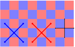
(a) The chessboard coloring holds within three square lattices: $(\mathbb{Z}^{2})_{\mathrm{even}}$ (blue dots and lines), $(\mathbb{Z}^{2})_{\mathrm{odd}}$ (red dots and lines) and the medial lattice $\hat{L}$ (black dots and lines).

(b) The modified medial lattice $L$ is formed when every vertex of $\hat{L}$ is replaced by a square. The dual lattice of $L$ is called bathroom tiling for obvious reasons.

(c) An admissible domain: here $c_{1}$ and $c_{2}$ agree on the beginning and end and they are otherwise avoiding each other and the domain they cut from the bathroom tiling has boundary consisting of two monochromatic arcs.

Figure 9: Modified medial lattice and its admissible domain.

Let $\hat{L}=(\mathbb{Z}+1/2)^{2}$, i.e., the graph formed by the vertices and the edges of the colored squares in the chessboard coloring. It is called the medial lattice of $(\mathbb{Z}^{2})_{\mathrm{even}}$ and its dual $(\mathbb{Z}^{2})_{\mathrm{odd}}$. Note that vertices of $\hat{L}$ are exactly those points where an edge of $(\mathbb{Z}^{2})_{\mathrm{even}}$ and an edge of $(\mathbb{Z}^{2})_{\mathrm{odd}}$ intersect.

It is useful to modify the medial lattice slightly. At each vertex of $\hat{L}$ position a white square so that the corners are lying on the edges of $\hat{L}$. The size of the square can be chosen so that the resulting blue and red octagons are regular. See Figure 9(b). Denote the graph formed by the vertices and the edges of the octagons by $L$ and call it modified medial lattice of $(\mathbb{Z}^{2})_{\mathrm{even}}$ (or $(\mathbb{Z}^{2})_{\mathrm{odd}}$). The dual of $L$, i.e. the blue and red octagons and the white squares (or rather their centers), is called the bathroom tiling.

Similarly, it is possible to define the modified medial lattice of a general planar graph $G$. For each middle point of an edge put a vertex of $\hat{L}$. Go around each vertex of $G$ and connect any vertex of $\hat{L}$ to its successor by an edge. The resulting graph is the medial graph. Notice that each vertex has degree four and hence it is possible to replace each vertex by an quadrilateral. The result is the modified medial lattice.

4.1.3 Admissible domains

Suppose that we are given two paths $(c_{j}(k))$, $j=1,2$, on the modified medial lattice and $k$ runs over the values $0,1,\ldots,n_{j}$, that satisfy the following properties:

• Each $c_{j}$ is simple and has only blue and white faces of the bathroom tiling on its one side and red and white faces on the other side.

• The first (directed) edges $(c_{j}(0),c_{j}(1))$ coincide and the edge is between a blue and a red face. Denote by $a$ the common starting point of $c_{j}$, $j=1,2$.

• The last edges $(c_{j}(n_{j}-1),c_{j}(n_{j}))$ coincide and the edge is between a blue and a red face. Denote by $b$ the common ending point of $c_{j}$, $j=1,2$.

• The paths $c_{j}$ may have arbitrarily long common beginning and end parts, but otherwise they are avoiding each other.

• The unique connected component of $\mathbb{C}\setminus\bigcup\hat{c}_{j}$ which is bounded, has $a$ and $b$ on its boundary, where $\hat{c}_{j}$ is the locus of the polygonal line corresponding to vertices $c_{j}(k)$, $0\leq k\leq n_{j}$. Denote this component by $U=U(c_{1},c_{2})$.

Let’s call a pair $(c_{1},c_{2})$ satisfying these properties an admissible boundary and $U=U(c_{1},c_{2})$ is called admissible domain. Let’s use a shortened notation that $U$ contains the information how $c_{1}$ and $c_{2}$ or $a$ and $b$ are chosen.

Suppose that $(\gamma(k))_{0\leq k\leq l}$ is a path on the modified medial lattice that starts from $a$ and possibly ends at $b$ but is otherwise avoiding $c_{1}$ and $c_{2}$. Suppose also that $\gamma$ has the property that it has only blue and white faces on one side and only red and white faces on the other side. Call this kind of path admissible path. If $\gamma(k)$, $0\leq k\leq 2m<l$ and $c_{j}$ are concatenated in a natural way (they have only one common point $a$) as a curve from $\gamma(2m)$ to $b$ and this curve is denoted as $c_{j,2m}$, then the pair $(c_{1,2m},c_{2,2m})$ is an admissible boundary.

Later it will be useful to consider the following object. Define generalized admissible domain with $2n$ marked boundary points or simply $2n$-admissible domain as the $U(c_{1},c_{2},\ldots,c_{2n})$ as the bounded component of $\mathbb{C}\setminus(\hat{c}_{1}\cup\ldots\cup\hat{c}_{2n})$ where $c_{j}$ are simple paths on $L$ so that $c_{2k-1}$ and $c_{2k}$ agree on the beginning and $c_{2k}$ and $c_{2k+1}$ on the end (here use cyclic order so that $c_{2n+1}=c_{1}$) and otherwise as above. For example, we require the marked points $c_{1}(0),c_{1}(n_{1}),c_{3}(0),c_{3}(n_{3}),\ldots$ to be on the boundary of $U(c_{1},c_{2},\ldots,c_{2n})$.

4.1.4 Advantages of the definitions

Now the advantages of the above definitions are the following:

• It is easier to deal with simple curves on the discrete level. This is the primary motivation of considering the modified medial lattice.

• As noted above, if we start from an admissible boundary and follow an admissible curve, then the pair $(c_{1,2m},c_{2,2m})$ stays as an admissible boundary. It is practical to have a stable class of domains in that sense.

• Let $(\pi(t)_{0\leq t\leq l})$ be the polygonal curve corresponding to $(\gamma(k))$ so that $\pi(k)=\gamma(k)$ and the parametrization is linear on the intervals $[k,k+1]$. Then the points of $\pi$ are bounded away from the boundary $\partial U=\hat{c}_{1}\cup\hat{c}_{2}$ except near the end points, that is,

  $$\mathrm{d}(\pi(t),\partial U)\geq 2\eta\quad\text{when }1\leq t\leq l-1$$

  and similarly the points on

  $$\mathrm{d}(\pi(t),\pi(s))\geq 2\eta\quad\text{when }|t-s|\geq 1$$

  here $\eta>0$ is a constant depending on the lattice. Later, we can use this to deal with the scales smaller than $\eta$ when checking the condition.

4.1.5 FK model on the square lattice

Let $U=U(c_{1},c_{2})$ be an admissible domain and assume that the octagons along $c_{1}$ (inside $U$ away from the common part with $c_{2}$) are blue. Denote by $G=G(c_{1},c_{2})\subset(\mathbb{Z}^{2})_{\mathrm{even}}$ the graph formed by the centers of the blue octagons inside $U$ and by $E_{W}$ the blue edges along $c_{1}$. $E_{W}$ is connected and it will be the set of wired edges. Let $G^{\prime}$ be the planar dual of $G$, that is, the graph formed by the centers of the red octagons inside $U$. Let $G_{L}$ be the subgraph of $L$ formed by the vertices in $U\cup\{a,b\}$ and edges which stay inside $U$.

For each $0<p<1$, $q>0$, define a probability measure on $\Omega=\Omega(c_{1},c_{2})=\{\omega\in\{0,1\}^{E(G)}:\omega=1\textnormal{ on }E_{W}\}$ by

$$\mu_{U}^{p,q}=\mu_{G,E_{W}}^{p,q}$$ (83)

The setup is illustrated in Figure 10. There is a natural dual $\omega^{\prime}$ of $\omega$ defined on $E(G^{\prime})$ such that for each white square in $U$ the edge going through that square is open in $\omega^{\prime}$ if and only if the edge of $E(G)$ going through that square is closed in $\omega$. The duality between $\omega$ and $\omega^{\prime}$ is shown in Figures 10(a) and 10(b). Which of the two edges intersecting in a white square is open in $\omega$ or $\omega^{\prime}$ can be represented by coloring the square with that color. The picture then looks like Figure 10(c). The essential information of that picture is encoded in the set of interfaces, that is, one interface starting from and ending to the boundary, because of the boundary conditions, and several loops. These interfaces are separating open cluster of $\omega$ from open cluster of $\omega^{\prime}$. Moreover, there is one-to-one correspondence between $\omega$, $\omega^{\prime}$ and the interface picture. The random curve connecting $a$ and $b$ in the interface picture is denoted by $\gamma$ and its law by $\mathbb{P}_{U}$ when the values of $p$ and $q$ are otherwise known.

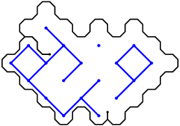
(a) A configuration of open edges on $G$ satisfying the wired boundary condition along $c_{1}$.

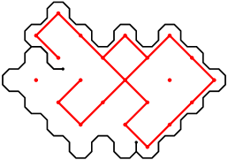
(b) The corresponding dual configuration of open edges on $G^{\prime}$. Note that it is wired along $c_{2}$.

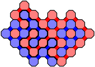
(c) Coloring of the squares with blue and red enables to define the collection of interfaces which separate the blue and red regions.

Figure 10: The correspondence between the configuration on $G$ (a), the configuration on $G^{\prime}$ (b) and the interfaces and the coloring of the squares (c).

It is generally known that the probability measure $\mu_{U}^{p,q}$ can be written in the form

$$\mu_{U}^{p,q}(\omega)=\frac{1}{Z^{\prime}}\left(\frac{p}{(1-p)\sqrt{q}}\right)^{|\omega|}(\sqrt{q})^{\textrm{number of loops}}.$$ (84)

From this it follows that

$$p_{\mathrm{sd}}(q)=\frac{\sqrt{q}}{1+\sqrt{q}}$$ (85)

is a self-dual value of $p$. When $p=p_{\mathrm{sd}}$, the quantity inside the first brackets is equal to $1$, and it doesn’t make difference whether the model was originally defined in $G$ or $G^{\prime}$. Both give the same probability for the configuration of Figure 10(c). It turns out that the self-dual value $p=p_{\mathrm{sd}}$ is also the critical value at least for $q\geq 1$, see [4].

4.1.6 Verifying Condition G2 for the critical FK Ising

For each admissible domain $U$ (and for each choice of $a$ and $b$) define a conformal and onto map $\phi_{U}:U\to\mathbb{D}$ such that $\phi_{U}(a)=-1$ and $\phi_{U}(b)=1$. In this subsection, the following result will be proven.

Proposition 4.3.

Let $\mathbb{P}_{U}$ be the law of the critical FK Ising interface in $U$, i.e., $\mathbb{P}_{U}$ is the law of $\gamma$ under $\mu_{U}^{p_{\mathrm{sd}},2}$. Then the collection

$$\Sigma_{\textnormal{FK Ising}}=\left\{\left(\phi_{U},\mathbb{P}_{U}\right)\;:\;U\textnormal{ admissible domain}\right\}$$ (86)

satisfies Condition G2.

Remark 4.4.

In a typical application, a sequence $U_{n}$ of admissible domains and a sequence of positive numbers $h_{n}$ are chosen. Then the family

$$\Sigma=\left\{\delta_{n,*}\left(\phi_{U_{n}},\mathbb{P}_{U_{n}}\right)\;:\;n\in\mathbb{N}\right\}$$ (87)

also satisfies Condition G2, where $\delta_{n,*}$ is the pushforward map of the scaling $z\mapsto h_{n}\,z$. The scaling factors $h_{n}$ play no role in checking Condition G2.

We postpone the proof of Proposition 4.3 until the required tools have been presented.

Consider a $4$-admissible domain $U=U(c_{1},c_{2},c_{3},c_{4})$ such that $c_{1}$ and $c_{3}$ are wired arcs. Let the marked points be $a_{j}$, $j=1,2,3,4$, in counterclockwise direction and assume that $a_{1}$ and $a_{2}$ lie on $c_{1}$ and $a_{3}$ and $a_{4}$ lie on $c_{3}$. Then there is a unique conformal mapping $\phi_{U}$ from $U$ to $\mathbb{H}$ such that $b_{j}=\phi(a_{j})\in\mathbb{R}$ satisfy

$$b_{1}<b_{2}<b_{3}<b_{4},\quad b_{2}-b_{1}=b_{4}-b_{3},\quad b_{2}=-1\quad\text{and}\quad b_{3}=1.$$

A sequence of domains $U_{n}$ is said to converge in the Carathéodory sense if the mappings $\phi_{U_{n}}^{-1}$ converge uniformly in the compact subsets of $\mathbb{H}$.

An open path is a path of open edges of $\omega$. For any 4-admissible domain $U$ we say that $U$ is crossed by an open path if there is an open path which connects the wired arcs. Denote this event by $O(U)$. More generally on any graph we can talk about open crossing of a set vertices with two specified subsets, which we call “sides”. This means that in the configuration $\omega$ there is an open path connecting the sides within this set. Open crossings and crossings by the interface are different but in some cases related events — this fact will be used below.

Proposition 4.5.

Let $U_{n}=h_{n}\hat{U}_{n}$ be a sequence of domains such that the sequence of reals $h_{n}\searrow 0$ and $\hat{U}_{n}$ is a sequence of 4-admissible domains. If the sequence $U_{n}$ converges to a quadrilateral $(U,a,b,c,d)$ in the Carathéodory sense as $n\to\infty$, then $\mathbb{P}_{n}[O(\hat{U}_{n})]$ converges to a value $s\in[0,1]$. If $(U,a,b,c,d)$ is non-degenerate then $0<s<1$. Here $\mathbb{P}_{n}$ is the probability measure $\mu_{\hat{U}_{n},P}^{p_{\mathrm{sd}},2}$ where $P$ is a fixed partitioning of the set $\{1,2\}$.

This proposition is proved in [11] for general isoradial graphs with an exact formula based on discrete holomorphicity. The following is a direct consequence of Proposition 4.5.

Corollary 4.6.

If $(U,a,b,c,d)$ is non-degenerate then there are $\varepsilon>0$ and $n_{0}>0$ so that $\varepsilon<\mathbb{P}_{n}[O(\hat{U}_{n})]<1-\varepsilon$ for any $n>n_{0}$.

Finally before giving the proof of Proposition 4.3, we state the following conditional theorem which is likely to be useful for FK models with $q\neq 2$. The proof is exactly the same as for Proposition 4.3. In fact, Condition G2 is verified for $1\leq q\leq 4$ in [12] based on this type of estimates.

Proposition 4.7.

Let $\mathbb{P}_{U}$ be the law of the critical FK model interface in $U$, i.e., $\mathbb{P}_{U}$ is the law of $\gamma$ under $\mu_{U}^{p_{\mathrm{sd}},q}$ for $q\geq 1$. If the statement of Corollary 4.6 holds for the critical FK model with the parameter $q$, then the collection

$$\Sigma_{\textnormal{FK(q)}}=\left\{\left(\phi_{U},\mathbb{P}_{U}\right)\;:\;U\textnormal{ admissible domain}\right\}$$ (88)

satisfies Condition G2.

We establish below one of the geometric conditions and not directly one of the conformally invariant conditions. The reason for this is that we want to apply Corollary 4.6 only a finite number of times. To verify the conformally invariant condition directly, we would have to use some compactness property for the family of quadrilaterals. This might be more or less equivalent to the proof below.

Proof of Proposition 4.3.

Let’s use the continuous time parametrization of $\gamma$ with constant speed so that $\gamma(n)$ is a lattice point of $L$ if and only if $n$ is an integer (between $0$ and $l$). Notice that on even time instances $\gamma(2n)$ is in a crossing “arriving” to a white square and it chooses left or right turn depending on the color revealed on the square, in the sense of Figure 10(c). The filtration generated $\mathcal{F}_{t}$ by $\gamma(s)$, $s\leq t$, (or the finer filtration made by adding an infinitesimal peek to the future) remains constant on $t\in(2n,2n+2)$ where $n$ is an integer. Hence we can restrict to the case $t=2n$, $n$ an integer. Then $U_{t}=U\setminus\gamma[0,t]$ is an admissible domain.

This simplifies the proof a lot. Instead of considering all $t=2n$ we will consider $t=0$ and all admissible domains. In other word, we don’t have to consider any stopping times below, but instead we have to consider all possible admissible domains. But luckily this was the set of domains we used in the definition of $\Sigma_{\textnormal{FK Ising}}$.

We can also assume that $r>\eta$ where $\eta$ is as in the section 4.1.4. In the complementary case, we notice that no disc of the form $B=B(z_{0},r)$, where $0<r\leq\eta$ and which intersects the boundary of the domain, can contain any lattice points of $L$ which are in the interior of the domain. Also choose $C>0$ such that there are no trivialities such as an edge crossing $A(z_{0},r,R)$ for some $z_{0}$ and $r>\eta$ and $R>Cr$.

Let $U$ be an admissible domain and $G(U)\subset(\mathbb{Z}^{2})_{\textnormal{even}},G^{\prime}(U)\subset(\mathbb{Z}^{2})_{\textnormal{odd}},G_{L}(U)\subset L$ the corresponding graphs, and let $c_{1}$ and $c_{2}$ be the two marked boundary arcs as in Section 4.1.3. Let $A=A(z_{0},r,R)$ be an annulus such that $r>\eta$. Write $\mu_{1}=\mu_{U}^{p_{\mathrm{sd}},2}$. Write the set $A^{u}$, which is defined as in (3), as a disjoint union $A^{u}=U_{1}\cup U_{2}$ where $U_{k}$ is next to $c_{k}$, that is, if we approach the boundary of the domain by a sequence in $U_{k}$, we hit $c_{k}$ (say, in the conformal sense after mapping to a reference domain with simple boundary). See also Figure 11.

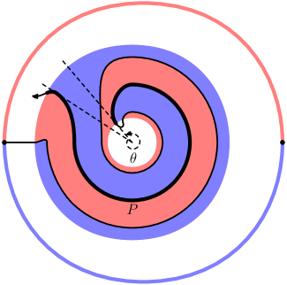
Figure 11: The boundary of the domain $U$ is the black solid line and the boundary arcs $c_{1}$ and $c_{2}$ have the solid blue and red lines, respectively, next to them. The parts $U_{1}$ and $U_{2}$ of $A^{u}$ are colored with slanted lines. They are the regions colored with blue and red, respectively. The boundary of $U_{1}$ is wired and the boundary of $U_{2}$ is dual wired. As one boundary arc $P$ is fixed the components are in the $2\pi$ sector starting from that curve. The angle $\theta$ is the difference of the maximum and minimum value of the angle variable defined continuously on $P$.

Since $\gamma$ is the interface which separates the cluster of open edges connected to $c_{1}$ from the cluster of dual open edges connected to $c_{2}$

$$\mathbb{P}_{U}(\gamma\textnormal{ crosses }A^{u})$$

$$\leq\mu_{1}(\textnormal{open crossing of }U_{1}\textnormal{ or dual open crossing of }U_{2})$$

$$\leq\mu_{1}(\textnormal{open crossing of }U_{1})+\mu_{1}(\textnormal{dual open crossing of }U_{2})$$

$$\leq 2K$$

where $K$ is the maximum of the two terms on the preceding line. Therefore we have to prove that $K<1/4$. By symmetry, it is enough to prove that

$$\mu_{1}(\textnormal{open crossing of }U_{1})<1/4.$$ (89)

Let’s define two discrete versions of the annulus $A$ on the modified medial lattice. The subset $A_{\text{blue}}\subset A$ is a doubly connected domain in $\mathbb{C}$. We require that the boundary of $A_{\text{blue}}$ is a path in the modified medial lattice and that the faces of the modified medial lattice inside $A_{\text{blue}}$ next to its boundary are blue or white. We also require that $A_{\text{blue}}$ is maximal such domain with respect to taking unions. Similarly, let $A_{\text{red}}$ be the maximal subdomain of the annulus $A$ that has red and white boundary on the modified medial lattice. In other words, $A_{\text{blue}}$ and $A_{\text{red}}$ are discrete approximations of $A$, with correct type of boundary. Let $V_{-}$ and $V_{+}$ be the connected components of the boundary vertices on $A_{\text{blue}}$ and denote by $V_{-}\leftrightarrow V_{+}$ the event that there is an open path between $V_{-}$ and $V_{+}$ in the given graph. Let $G_{2}\subset G$ be the subgraph corresponding to the domain $U_{1}\cap A_{\text{blue}}$. Let $E_{2}\subset E(G_{2})$ be the set of blue edges along the boundary. Let $\mu_{2}$ be the random cluster measure on $G_{2}$ such that the edges in $E_{2}$ are wired and all the components of $E_{2}$ are counted to be separate. Then by considering $f=\mathbbm{1}_{E_{2}\subset\omega}$ in the FKG inequality we have that

$$\mu_{1}(\textnormal{open crossing of }U_{1})\leq\mu_{2}\left(V_{-}\leftrightarrow V_{+}\right).$$

Similarly, it is enough to prove there is a constant $s<1$ such that

$$\mu_{2}\left(V_{-}\leftrightarrow V_{+}\right)\leq s$$ (90)

for a fixed ratio $R/r$ since using this in several concentric annuli we get (89) for a larger annulus. Yet another similar argument shows that we can consider only annuli $A(z_{0},r,R)$ where $r>C^{\prime}\eta$ for any fixed $C^{\prime}\geq 1$. Namely, if (89) holds for $r>C^{\prime}\eta$ then for $\eta<r\leq C^{\prime}\eta$ we can ignore the part below the scale $C^{\prime}\eta$ and only consider crossing between $R$ and $C^{\prime}\eta$ and then we notice that $R\geq Cr>(C/C^{\prime})\cdot(C^{\prime}\eta)$ and therefore by modifying the value $C$ we get (89) for the whole range of $r$. Therefore we will prove (90) when $r>C^{\prime}\eta$ when $C^{\prime}$ is suitably chosen and $R/r$ fixed.

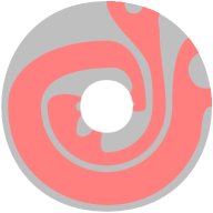
(a) The domain $U_{1}$.

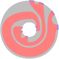
(b) In the measure $\mu_{2}$ the edges along the boundaries of the annulus are wired.

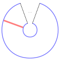
(c) In the case $\theta\leq 4\pi$, the final domain to be considered is a $6\pi$ opening in the annulus with wired edges along the boundaries if the annulus. The blue color indicates the wired edges and the red color the dual wired edges. The crossing is between the two blue boundary components.

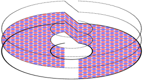
(d) A schematic illustration how to cover the annulus with infinitely many layers of the lattice.

Figure 12: Illustration how the FKG inequality is applied here in general and especially in the case $\theta\leq 4\pi$.

Let $P$ be one of the boundary arcs of $U_{1}$ which cross $A$. Write the points $z\in P$ in polar coordinates $z=z_{0}+\rho e^{i\xi}$ so that $\xi$ is continuous along $P$. Denote by $\theta$ the difference between the maximum and the minimum value of $\xi$ along $P$ and by $\alpha$ the minimum value of $\xi$. The value of $\alpha$ is determined only up to additive multiple of $2\pi$ but $\theta$ is unique. Now $\xi$ spans the interval $[\alpha,\alpha+\theta]$ along $P$. The rest of the proof is divided into two cases: $\theta\leq 4\pi$ and $\theta>4\pi$.

Case $\theta\leq 4\pi$: Consider the right half-plane $\mathbb{H}_{1}=\{(\rho,\xi):\rho>0,\xi\in\mathbb{R}\}$ as an infinite covering surface of $\mathbb{C}\setminus\{z_{0}\}$ such that $(\rho,\xi)\in\mathbb{H}_{1}$ gets projected on $z_{0}+\rho\,e^{i\xi}\in\mathbb{C}\setminus\{z_{0}\}$. Lift the lattice $L$ to $\mathbb{H}_{1}$ using this mapping locally in neighborhoods where it is a bijection and define $S_{\text{blue}}$ as the lift of $A_{\text{blue}}$, that is, as the maximal subdomain of $S=S(r,R)=\{(\rho,\xi):0<\rho<R,\xi\in\mathbb{R}\}$ such that the boundary is on the medial lattice and it is a blue boundary. Let $G_{3}$ be the subgraph of the lifted $(\mathbb{Z}^{2})_{\text{even}}$ corresponding to the domain $S_{\text{blue}}\cap(r,R)\times(\alpha,\alpha+6\pi)$ and denote the edges along the vertical boundary as $E_{3}$. Let $\mu_{3}$ be the random-cluster measure on $G_{3}$ where $E_{3}$ is wired and the components of $E_{3}$ are counted to be separate. Now $G_{2}$ can be seen as a subgraph of $G_{3}$. If the wired edges of the dual of $G_{2}$ are denoted by $E_{2}^{\prime}$, then applying the FKG inequality for the decreasing event $\{\omega\,:\,E_{2}^{\prime}\subset\omega^{\prime}\}$ and for the measure $\mu_{3}$ shows that

$$\mu_{2}\left(V_{-}\leftrightarrow V_{+}\right)\leq\mu_{3}\left(V_{-}\leftrightarrow V_{+}\right).$$

At this point we have reduced the problem to the event of an open crossing of fixed shape (independent of the domain we started with), but with variable size. Figure 12(c) illustrates how this shape looks like. Since this domain is a 4-admissible domain, we can use Proposition 4.5 to show that there are constants $C_{1}\geq 1$ and $s_{1}<1$ such that the right-hand side of the previous inequality is less than $s_{1}$ uniformly for any $r\geq C_{1}\eta$ and $R=3r$.

The previous statement follows if we are able to show that probability of an open crossing remains bounded away from one when we consider larger and larger $r$. This follows claim from the following argument. Make a counter assumption that there exists a sequence $\alpha_{n}\in[0,2\pi]$ and $r_{n}\to\infty$ such that if we set $m_{n}=\mu_{3}(V_{-}\leftrightarrow V_{+})$ in the domain $U_{3,n}$ with $r=r_{n}$, $R=3r_{n}$ and $\alpha=\alpha_{n}$ and $\theta=6\pi$, then $m_{n}\to 1$ as $n\to\infty$. By choosing a subsequence we can assume that $\alpha_{n}$ converges. Now the sequence of domains $r_{n}^{-1}U_{3,n}$ converges in the same sense as in Proposition 4.5 and hence $\lim_{n\to\infty}m_{n}<1$.

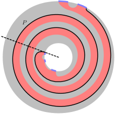
(a) $\mu_{2}$

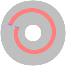
(b) $\mu_{4}$

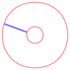
(c) $\mu_{5}$

Figure 13: Illustration how the FKG inequality is applied in the case $\theta>4\pi$.

Case $\theta>4\pi$: Similarly as in the other case define $S_{\text{red}}$ to be the lift of $A_{\text{red}}$ to $S$. Now note that any component of $G_{2}$ (view as lifted to $S$) intersects the radials $\alpha+2\pi$ and $\alpha+4\pi$ and any open crossing has to intersect those radial. Hence in the same way as above we can add blue boundary and blue wired edges to those radials and ignore the part outside $(r,R)\times(\alpha+2\pi,\alpha+4\pi)$. Denote the resulting graph by $G_{4}$ and the measure by $\mu_{4}$ and denote the vertices of the lifted $(\mathbb{Z}^{2})_{\text{even}}$ along those two radials by $V_{2\pi}$ and $V_{4\pi}$. Denote the dual wired edges of $\mu_{4}$ by $E_{4}^{\prime}$. Finally if $G_{5}$ is the graph corresponding to the domain $S_{\text{red}}\cap(r,R)\times(\alpha+2\pi,\alpha+4\pi)$ and $E_{5}$ are the boundary edges along the radials, then let $\mu_{5}$ be the random-cluster measure on $G_{5}$ with wired edges $E_{5}$. In the same way as above, we can apply the FKG inequality for $\mu_{5}$ and for the decreasing event $\{\omega\,:\,E_{4}^{\prime}\subset\omega^{\prime}\}$ to get the second inequality in

$$\mu_{2}\left(V_{-}\leftrightarrow V_{+}\right)\leq\mu_{4}\left(V_{2\pi}\leftrightarrow V_{4\pi}\right)\leq\mu_{5}\left(V_{2\pi}\leftrightarrow V_{4\pi}\right).$$

Again at this point we have reduced the problem to the event of an open crossing of fixed shape which is now illustrated in Figure 12(c). Use again Proposition 4.5 to show that there are constants $C_{2}\geq 1$ and $s_{2}<1$ such that the right-hand side of the previous inequality is less than $s_{2}$ uniformly for any $r\geq C_{2}\eta$ and $R=3r$.

When we combine these separate cases, the claim follows for $s=\max\{s_{1},s_{2}\}$ and $C^{\prime}=\max\{C_{1},C_{2}\}$. ∎

4.2 Spin Ising model

Consider the spin Ising model at criticality on the square lattice (or any isoradial graph) with Dobrushin boundary conditions.

In [11] a discrete holomorphic observable $f_{\delta}(z)=f_{\delta}^{U_{\delta},a_{\delta},b_{\delta}}(z)$ is constructed with a martingale property. It is shown in Theorem 5.6 that, as the mesh $\delta$ of the lattice tends to zero, the discrete domains $U_{\delta}$ with marked points $a_{\delta},b_{\delta}$ tend to a continuum domain $(U,a,b)$, the observable converges to its continuous counterpart $f(z)=f^{U,a,b}(z)$. The latter is given by a solution of the Riemann-Hilbert boundary value problem, and can be written as $f=\sqrt{\Psi^{\prime}}$, where $\Psi$ is the conformal map of $U$ to the upper half-plane with $\Psi(a)=\infty$, $\Psi(b)=0$, appropriately normalized at $b$. The convergence is uniform inside the domain $U$, and on straight pieces of the boundary common to $U$ and $U_{\delta}$.

Consider the interface (domain wall) joining the points $a_{\delta}$ and $b_{\delta}$ inside $U_{\delta}$. The results of [11] immediately imply convergence of the interface to SLE₃ in the sense of the Loewner driving functions convergence. In [10] it was shown how to use the results of the present article together with the crossing estimates of the article [9] to deduce the strong interface convergence (see Theorem 1.9 of the present article), by verifying the conditions of present article.

Below we sketch an alternative way to check Condition G2, using only the observable results of [11].

4.2.1 Fermionic observable of spin Ising model

The spin Ising model is defined on any finite graph $G=(V,E)$. The random configuration ${\underline{\sigma}}$ takes values in $\{-1,+1\}^{V}$ and its distribution is given by

$$\mathbb{P}_{\beta}[{\underline{\sigma}}=\underline{s}]=\frac{1}{Z}\exp\left(\beta\sum_{(v_{1},v_{2})\in E}s_{v_{1}}s_{v_{2}}\right).$$ (91)

for any $\underline{s}\in\{-1,+1\}^{V}$. Here the partition function $Z$ is the constant normalizing the measure to be a probability measure. The quantity $s_{v}$ is called the spin at $v$. The parameter $\beta>0$ is interpreted as the inverse temperature.

Consider the critical Ising model, $\beta=\beta_{c}$, on a finite, connected subgraph of the square lattice with mesh $\delta>0$. Then

$$\mathbb{P}_{\beta_{c}}[{\underline{\sigma}}=\underline{s}]=\frac{1}{\tilde{Z}}x_{c}^{n(\underline{s})}$$ (92)

where $n(\underline{s})=\#\{(v_{1},v_{2})\in E\,:\,s_{v_{1}}\neq s_{v_{2}}\}$ and $x_{c}=\sqrt{2}-1$. If we fix the spin at one vertex, there is a one-to-one correspondence between spin configurations and even subgraphs of the dual graph of $G$, given by the interfaces (domain walls) separating $+1$ and $-1$ spins.

Let $\mathcal{S}$ be the collection of even subgraphs of $G^{*}$, and $\mathcal{S}_{a,b}$ be the collection of subgraphs which are even everywhere except at $a$ and $b$, where they are odd. Any element in $S\in\mathcal{S}_{a,b}$ can be written as a pair $S=(\gamma,\Gamma)$ such that $\gamma$ and $\Gamma$ are edge-disjoint, $\gamma$ is a non-self-intersecting path from $a$ to $b$ and $\Gamma$ is an even graph. The representation is not unique, but we will fix it uniquely by taking $\gamma$ to be the left-most such path.

For $(\gamma,\Gamma)\in\mathcal{S}_{a,z}$ denote by $W(z,\gamma)$ the winding of $\gamma$ from $a$ to $z$. Define an observable

$$f_{\delta}(z)=f_{\delta}^{U,a,b}(z)=\nu\frac{\sum_{S=(\gamma,\Gamma)\in\mathcal{S}_{a,z}}x_{c}^{\#S}e^{-\frac{i}{2}W(z,\gamma)}}{\sum_{S=(\gamma,\Gamma)\in\mathcal{S}_{a,b}}x_{c}^{\#S}e^{-\frac{i}{2}W(b,\gamma)}}=\nu\frac{\sum_{S=(\gamma,\Gamma)\in\mathcal{S}_{a,z}}\;x_{c}^{\#S}e^{-\frac{i}{2}W(z,\gamma)}}{Z_{a,b}\,e^{-\frac{i}{2}W(b)}}$$ (93)

where in the last equation we use that when $a$ and $b$ are boundary points, the winding to $b$ doesn’t depend on $\gamma$. Here $Z_{a,b}$ is the partition function $\sum_{S\in\mathcal{S}_{a,b}}x_{c}^{\#S}$, the quantity $\#S$ is the number of edges in $S$ and $\nu$ is a constant. The constant $\nu$ depends on local shape of the domain $U$ near $b$, but it takes a fixed value over the class of subdomains of $U$ that we will consider.

Theorem 4.8 (Chelkak–Smirnov [11]).

Let $U$ be a simply connected domain and let $b$ be a boundary point of $U$. Assume that the boundary of $U$ is straight near $b$ and $U$ contains a rectangular neighborhood $R$ of $b$. Then for an appropriate choice of the constant $\nu$, $f$ has both of the following properties:

1. For any $z$, $f_{\delta}(z)$ is a martingale with respect to the growing interface.

2. As $\delta\to 0$, $f_{\delta}$ converges to $\lambda\sqrt{\Psi^{\prime}}$, uniformly on any compact subset of $U$ and uniformly in any straight part of $\partial U$, where $\Psi$ is a conformal map from $U$ to $\mathbb{H}$ with $\Psi(b)\in\mathbb{R}$ and $|\Psi^{\prime}(b)|=1$ and $\lambda$ is fixed constant with unit modulus.

Moreover once $b$ and $R$ are fixed, the convergence of $f_{\delta}^{U,a,b}$ in (ii) is uniform over all domains $U$ as well as points $a$ and $z$, as long as $a$ is at a finite distance from $R$ and $z$ is inside $R$.

Remark 4.9.

Although $\Psi$ is only unique up to an additive constant, $\Psi^{\prime}$ is uniquely determined. The branch of the square root and the constant $\lambda$ are chosen so that $\lambda\sqrt{\Psi^{\prime}}$ is positive at $b$. Denote by $f=f^{U,a,b}$ the function

$$f^{U,a,b}=\lambda\sqrt{\Psi^{\prime}}.$$ (94)

4.2.2 Using monotonicity and the martingale observable

Consider a triplet $(U,a,b)$ and an annulus $A=A(z_{0},r,R)$. We aim to verify Condition G2 for spin Ising model on the domain $(U,a,b)$ with respect to the annulus $A$. To that effect we consider the random curve $\gamma$ which is the interface separating the macroscopic $+1$ and $-1$ clusters in the domain $U$ with Dobrushin boundary conditions which change at $a$ and $b$.

Remember that $A^{u}$ is defined as in (3). Let $V_{k}$, $k=1,2,\ldots,n$, be the connected components of $A^{u}$ which can be crossed by the curve without first crossing some other connected component of $A^{u}$. We can assume that all $V_{k}$ have boundary conditions $-1$ and that any crossing of $V_{k}$ has to first go from the outer circle to the inner circle of $\partial A$. The $+1$ boundary components or the components that go from inside to outside could be dealt with in identical manner.

Next we observe in the same way as in the case of FK Ising model that one of the two cases occurs: either all $V_{k}$ can be lifted simultaneously to the universal cover

$$F=\{(\rho,\theta)\in[r,R]\times\mathbb{R}\}$$ (95)

of $A$ so that they are in a sector of $6\pi$ opening in $F$, or that each of $V_{k}$ crosses a $2\pi$ sector in the angular direction. Basically, this division is possible since when we fix an arc of $\partial U$ that crosses $A$, its winding around $z_{0}$ is either less than $4\pi$ or greater than $4\pi$. In the first case, when we take the radial line through the point of the arc with smallest angle, then all $V_{k}$ lie in the $6\pi$ sector from it. In the second case, we can similarly find a $2\pi$ sector that all $V_{k}$ cross. We will deal with the first case here explicitly. The other case is similar.

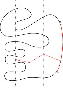
(a) The domain in “logarithmic coordinates”, that is, in order to get back to the original domain we need to apply the covering map $w\mapsto z_{0}+e^{w}$. The annulus is the vertical strip drawn with dots. We wish to give an upper bound to the probability of the event of a connected path of $+1$ spins crossing the annulus (or more accurately any of its components with purely $-1$ boundary), indicated by the dashed red arrow.

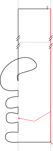
(b) The domain after the transformation. The horizontal dotted line is the middle radial line of the sector. By monotonicity, the upper bound is given as the probability of having a connected path of $+1$ spins crossing the lower half of the sector. The fact that the crossing is bounded away from $b$ is useful for technical purposes when using Theorem 4.8.

Figure 14: We apply a transformation to the domain which is consistent with the monotonicity of the Ising model. The transformed domain is a simply connected subdomain of an appropriately chosen Riemann surface. Thus any of the hanging parts to the left of the annulus in 14(b) which seem to overlap with the part of the domain in the annulus should be considered to be on a different sheet of the cover than the annular part. Notice that in 14(b) we require that the crossing is in the lower half.

We apply the transformation illustrated in Figure 14 to the domain $(U,a,b)$. We’ll give the details in next paragraphs.

Let $I_{j}$, $j=1,2,\ldots,m$, be the boundary arcs of $V_{k}$ that lie on the circle of radius $r$ and centered at $z_{0}$, that is, on the inner boundary of $A$. And for each $j=1,2,\ldots,m$, let $U_{j}$ be the connected component of $U\setminus I_{j}$ which is disconnected from $a$ and $b$ in $U$ by $I_{j}$.

Suppose that the interface in $(U,a,b)$ makes an unforced crossing of $A$. Then in particular, there is a crossing of $+1$ spins from the $+1$ boundary arc to one of the components $U_{j}$. By monotonicity of the Ising model, the probability of such an event increases if we pull the “$+1$ boundary” closer and push the “$-1$ boundary” away.

Consider the $12\pi$ sector on the universal cover to which we can lift all $V_{k}$ so that they are lifted to the “lower” half (opening of $6\pi$) of the $12\pi$ sector. Below we will always consider crossings that stay in the “lower” half. Let $U^{\medsquare}_{0}\subset F$ be the $12\pi$ sector and let $U^{\#}_{0}\subset F$ be its discrete approximation, say, let $U^{\#}_{0}\subset F$ be the union of all the faces of the lifted square lattice that are contained in $U^{\medsquare}_{0}$. Denote by $U^{\medsquare}$ and $U^{\#}$ the domain and its discrete approximation which we get by gluing each $U_{j}$ along the lifted arcs $I_{j}$ to $U^{\medsquare}_{0}$ and $U^{\#}_{0}$, respectively, on appropriate Riemann surfaces so that $U_{j}$ remain disjoint from $U^{\medsquare}_{0}$ and $U^{\#}_{0}$. See Figure 14 for illustration.

Let $a^{\#}$ be one of the boundary points of the dual lattice near one of the corners of $U^{\#}_{0}$ corresponding to $\rho=R$ and let $b^{\#}$ be close to the other corner, but next to a point with $\rho=9R/10$. Here $\rho$ refers to the coordinates (95). Suppose that the radial angle of $a^{\#}$ is smaller than the radial angle of $b^{\#}$. If the boundary condition change at $a^{\#}$ and $b^{\#}$ from $-1$ to $+1$ and back in this new setup, then the probability of the $+1$ crossing from $a^{\#}b^{\#}$ to any of $U_{j}$, and which stays in “lower half”, gives an upper bound to the probability of an unforced crossing of $A$ in $(U,a,b)$ by monotonicity of the Ising model (FKG inequality).

This means that the interface in the new setup will make a crossing staying in the “lower half” of $U^{\#}_{0}$ to some $U_{j}$. The probability of this can be estimated using the martingale property of $f$.

Let $a^{\medsquare}$ and $b^{\medsquare}$ be the boundary points of $U^{\medsquare}$ that correspond to $a^{\#}$ and $b^{\#}$.

Let $c^{\#}$ be on the same radial boundary segment of $U^{\#}$ as $b^{\#}$ and let $c^{\medsquare}$ be the corresponding boundary point of $U^{\medsquare}$. Since $\lambda\sqrt{\Psi^{\prime}(b^{\medsquare})}$ is positive and the boundary near $b$ is straight, also $\lambda\sqrt{\Psi^{\prime}(c^{\medsquare})}$ is positive as well as any $f_{\delta}^{U^{\#}_{\tau},a^{\#}_{\tau},b^{\#}}(c^{\#})$ which we consider below. We define $a^{\#}_{\tau}$ to be the tip of $\gamma$ at the random time $\tau$ and $U^{\#}_{\tau}$ to be $U^{\#}\setminus\gamma[0,\tau]$. The domain $U^{\medsquare}_{\tau}$ is $U^{\medsquare}\setminus([a^{\medsquare},a^{\#}]\cup\gamma[0,\tau])$ where $[a^{\medsquare},a^{\#}]$ is the line segment from $a^{\medsquare}$ to $a^{\#}$ in the plane. Let $\tau$ be the hitting time of $\bigcup_{j>0}U_{j}$ by $\gamma$ and $U^{\#,-}_{0}$ be the “lower half” of $U^{\#}_{0}$. By the martingale property

$$f_{\delta}^{U^{\#},a^{\#},b^{\#}}(c^{\#})\geq\mathbb{E}\left[\mathbbm{1}_{\tau<\infty,\;\gamma[0,\tau]\subset U^{\#,-}_{0}}\;f_{\delta}^{U^{\#}_{\tau},a^{\#}_{\tau},b^{\#}}(c^{\#})\right].$$ (96)

Therefore to get an estimate for $\mathbb{P}[\tau<\infty,\;\gamma[0,\tau]\subset U^{\#,-}_{0}]$ we have to estimate the ratio

$$\frac{f_{\delta}^{U^{\#}_{\tau},a^{\#}_{\tau},b^{\#}}(c^{\#})}{f_{\delta}^{U^{\#},a^{\#},b^{\#}}(c^{\#})}$$

By the convergence of $f_{\delta}^{U^{\#},a^{\#},b^{\#}}(c^{\#})$ to $f^{U^{\medsquare},a^{\medsquare},b^{\medsquare}}(c^{\medsquare})$, we can choose a constant $\delta_{1}>0$ such that

$$f_{\delta}^{U^{\#},a^{\#},b^{\#}}(c^{\#})\leq 2f^{U^{\medsquare},a^{\medsquare},b^{\medsquare}}(c^{\medsquare})$$

for all $0<\delta<\delta_{1}$. By the uniform convergence of $f_{\delta}^{U^{\#}_{\tau},a^{\#}_{\tau},b^{\#}}(c^{\#})$ to $f^{U^{\medsquare}_{\tau},a^{\#}_{\tau},b^{\medsquare}}(c^{\medsquare})$ and by the fact that $f^{U^{\medsquare}_{\tau},a^{\#}_{\tau},b^{\medsquare}}(c^{\medsquare})$ is uniformly bounded below by a positive constant, we can choose a constant $\delta_{2}>0$ such that

$$f_{\delta}^{U^{\#}_{\tau},a^{\#}_{\tau},b^{\#}}(c^{\#})\geq\frac{1}{2}f^{U^{\medsquare}_{\tau},a^{\#}_{\tau},b^{\medsquare}}(c^{\medsquare})$$

for all $0<\delta<\delta_{2}$. Notice that we continue to denote the tip of the curve by $a^{\#}_{\tau}$ since it’s the tip of the discrete path $\gamma$ and in fact, $U^{\medsquare}_{\tau}$ is the continuum domain slitted by the discrete path.

Set $\delta_{0}=\min\{\delta_{1},\delta_{2}\}$. Then

$$\frac{f_{\delta}^{U^{\#}_{\tau},a^{\#}_{\tau},b^{\#}}(c^{\#})}{f_{\delta}^{U^{\#},a^{\#},b^{\#}}(c^{\#})}\geq\frac{1}{4}\frac{f^{U^{\medsquare}_{\tau},a^{\#}_{\tau},b^{\medsquare}}(c^{\medsquare})}{f^{U^{\medsquare},a^{\medsquare},b^{\medsquare}}(c^{\medsquare})}$$

for $0<\delta<\delta_{0}$.

Let $\psi$ be a conformal map that sends $U^{\medsquare}$ to $\mathbb{H}$ and $b^{\medsquare}$ to $\infty$ and such that its derivative at $b^{\medsquare}$ has modulus equal to $1$ in an appropriate sense. Then the function $\Psi$ in Theorem 4.8 and in (94) can be written as $\Psi=\eta_{\psi(a^{\medsquare})}\circ\psi$ where $\eta_{\alpha}:z\mapsto-(z-\alpha)^{-1}$. Notice also that $f^{U^{\medsquare}_{\tau},a^{\#}_{\tau},b^{\medsquare}}(c^{\medsquare})$ is a constant times the square root of the conformal map $\eta_{g(\psi(a^{\#}_{\tau}))}\circ g\circ\psi$ where $g$ is the conformal map sending $\mathbb{H}\setminus\psi([a^{\medsquare},a^{\#}]\cup\gamma[0,\tau])$ onto $\mathbb{H}$ and normalized hydrodynamically at $\infty$. Hence

$$\frac{f^{U^{\medsquare}_{\tau},a^{\#}_{\tau},b^{\medsquare}}(c^{\medsquare})}{f^{U^{\medsquare},a^{\medsquare},b^{\medsquare}}(c^{\medsquare})} =\sqrt{\frac{g^{\prime}(\psi(c^{\medsquare}))\;\eta_{g(\psi(a^{\#}_{\tau}))}^{\prime}(g(\psi(c^{\medsquare})))}{\eta_{\psi(a^{\medsquare})}^{\prime}(\psi(c^{\medsquare}))}}$$

$$=\sqrt{\frac{g^{\prime}(\psi(c^{\medsquare}))\;(\psi(c^{\medsquare})-\psi(a^{\medsquare}))^{2}}{(g(\psi(c^{\medsquare}))-g(\psi(a^{\#}_{\tau})))^{2}}}.$$ (97)

It remains to estimate the quantity inside the square root. We will do this in the next section.

4.2.3 Auxiliary results on conformal maps

We will slightly simplify the notation of the previous subsection.

Let $0<r<R$ and $\theta_{1}<\theta_{2}\leq\theta_{1}+2\pi k$, where $k\in\mathbb{N}$ is fixed. Let $U_{0}$ be an annular sector $U_{0}=\{(\rho,\theta)\in(r,R)\times(\theta_{1},\theta_{2})\}$, which we consider as a covering space of $A=A(z_{0},r,R)$ through the map $(\rho,\theta)\mapsto z_{0}+\rho e^{i\theta}$. Consider a domain $U$ which is simply connected and is obtained from $U_{0}$ by gluing (disjointly) to it along the radius $r$ boundary a finite number of $U_{j}$’s in an appropriate covering space as in the previous subsection.

Consider some numbers $0<r<r_{d}<r_{c}<R_{b}<R$. Set

$$a=z_{0}+Re^{i\theta_{1}},\qquad b=z_{0}+R_{b}e^{i\theta_{2}},$$

$$c=z_{0}+r_{c}e^{i\theta_{2}},\qquad d=z_{0}+r_{d}e^{i\theta_{2}},$$

where the proportionalities of $R$, $r_{c}$ and $r_{d}$ to $r$ are specified later, but we consider $R/R_{b}$ to be a fixed number close to $1$, say, equal to $9/10$. That is, $a,b,c,d$ follow the counterclockwise order on the boundary of the annular sector and $a$ is an outer corner of the sector, $b$ is close to the other corner and $b,c,d$ lie on the same ray. See Figure 15.

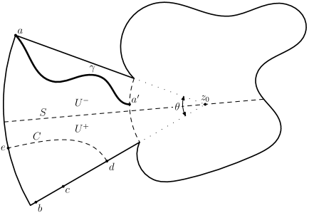
Figure 15: The setup for Lemma 4.10 and Proposition 4.11.

Let $S$ be the component of the intersection of $U$ and the line $\{z_{0}+te^{i(\theta_{1}+\theta_{2})/2}\,:\,t\in\mathbb{R}\}$ which meets the annular sector and hence ends at a point on the boundary of the annular section.

Let $\psi:U\to\mathbb{H}$ be conformal and onto such that $b$ is mapped to $\infty$. Let $C_{\mathbb{H}}$ be the half-circle in the upper-half plane centered at $\psi(a)$ and with the left-end point equal to $\psi(d)$. Set $C=\psi^{-1}(C_{\mathbb{H}})$. Denote $\psi(x)$ by $x_{\mathbb{H}}$ where $x=a,b,c,d$.

Define further disjoint connected domains $U^{\pm}$ such that $U=U^{-}\cup S\cup U^{+}$ and $U^{-}$ is next to $a$ and $U^{+}$ is next to $b$. Set also $U_{0}^{\pm}=U_{0}\cap U^{\pm}$.

Lemma 4.10.

There is a universal constant $m>1$, such that $C\subset U^{+}$ if $r_{d}>mr$.

Proof.

Denote the other endpoint of $C$ by $e$. By considering the modulus of the quad $(U,b,d,a,e)$ and using the conformal invariance of the modulus as well as the definition of $C_{\mathbb{H}}$, we see that $e\in\partial U^{+}$ for large enough $m$.

Now the path $C$ is characterized by the property that the boundary arcs $ed$ and $de$ of $U$ have both harmonic measure seen form any point of $C$ equal to $1/2$. We claim that on $S$ the harmonic measure of $de$ is strictly larger than that of $ed$. This is true in the domain obtained by gluing to $U_{0}$ along each $I_{j}$ the cover of $\mathbb{C}$ that is formed from infinite number of sheets glued along $I_{j}$. Notice that this is a space where $U$ can be embedded naturally. Here $I_{j}=\overline{U}_{0}\cap\overline{U}_{j}$. Since the harmonic measure of $de$ only increases when the domain is decreased, the claim holds for the general domain $U$. Thus the lemma follows. ∎

Proposition 4.11.

Consider a simple path $\gamma$ from $a$ to some $a^{\prime}$ with $|a^{\prime}-z_{0}|=r$. Denote $\psi(\gamma)$ by $\gamma_{\mathbb{H}}$ and $\psi(a^{\prime})$ by $a^{\prime}_{\mathbb{H}}$. Suppose that $\gamma$ is contained in $\overline{U_{0}^{-}}$. Let $H$ be $\mathbb{H}\setminus\gamma_{\mathbb{H}}$. Let $g:H\to\mathbb{H}$ be the Loewner map associated to $\gamma_{\mathbb{H}}$. Then for any $M>0$ there exists $N>0$ such that if $R/r\geq N^{3}$, $r_{c}=N^{2}r$, $r_{d}=Nr$, then

$$g^{\prime}(c_{\mathbb{H}})\;\frac{(c_{\mathbb{H}}-a_{\mathbb{H}})^{2}}{(g(c_{\mathbb{H}})-g(a^{\prime}_{\mathbb{H}}))^{2}}\geq M.$$ (98)

Proof.

Set $l=a_{\mathbb{H}}-d_{\mathbb{H}}$, which is the radius of the semicircle $C_{\mathbb{H}}$. Then $a_{\mathbb{H}}-c_{\mathbb{H}}>a_{\mathbb{H}}-d_{\mathbb{H}}=l$.

By considering the extremal length of suitable curve families, we can show that $0<g(a^{\prime}_{\mathbb{H}})-g(d_{\mathbb{H}})<g(d_{\mathbb{H}})-g(c_{\mathbb{H}})$ and that $0<d_{\mathbb{H}}-c_{\mathbb{H}}<\varepsilon l$ for $\varepsilon>0$ which can be arbitrarily small when $N$ is chosen to be large. In the former inequality the curve family is the family connecting $a^{\prime}b$ to $cd$ in $U\setminus\gamma$ and in the latter it is the family connecting $bc$ to $da$ in $U$, which both have small extremal length. By translating, we can assume that $a_{\mathbb{H}}=0$. Then $d_{\mathbb{H}}=-l$ and $c_{\mathbb{H}}=-l-l\tilde{\varepsilon}$ with $0<\tilde{\varepsilon}<\varepsilon$.

We observe that by the properties of Loewner flows $g(d_{\mathbb{H}})-g(c_{\mathbb{H}})<d_{\mathbb{H}}-c_{\mathbb{H}}=l\tilde{\varepsilon}$. That is, we can consider $g$ as a Loewner chain at the time corresponding to the value of its half-plane capacity and use the fact that $t\mapsto|g_{t}(x)-g_{t}(x^{\prime})|$ is decreasing for any real $x,x^{\prime}$ that lie on the same component of $\mathbb{R}\setminus\{W_{0}\}$, where $W_{0}$ is the Loewner driving term at time $0$.

The second observation coming from Loewner flows is that $g$ satisfies for all $\varepsilon>0$

$$g^{\prime}(c_{\mathbb{H}})\geq\tilde{g}^{\prime}(c_{\mathbb{H}})\geq\tilde{g}^{\prime}(-l-l\varepsilon)=\frac{(1+\varepsilon)^{2}-1}{(1+\varepsilon)^{2}}\geq 2\varepsilon-3\varepsilon^{2},$$

where $\tilde{g}(z)=z+l^{2}/z$. The first inequality follows from the fact that $g$ and $\tilde{g}$ can be seen as two time instances of the same Loewner chain and $t\mapsto g^{\prime}_{t}(x)$ for real $x$ is decreasing. The half-plane capacity of $g$ is less than that of $\tilde{g}$, which gives the order of the corresponding time instances.

Combining these estimates gives

$$g^{\prime}(c_{\mathbb{H}})\;\frac{(c_{\mathbb{H}}-a_{\mathbb{H}})^{2}}{(g(c_{\mathbb{H}})-g(a^{\prime}_{\mathbb{H}}))^{2}}\geq g^{\prime}(c_{\mathbb{H}})\;\frac{l^{2}}{(2l\tilde{\varepsilon})^{2}}\geq(2\varepsilon-3\varepsilon^{2})\;\frac{1}{4\varepsilon^{2}}=\frac{1}{2\varepsilon}-\frac{3}{4}.$$

And since $\varepsilon>0$ becomes arbitrarily small when $N$ is increased, the claim follows. ∎

Combining (96) and (97) with Proposition 4.11 gives Condition G2 for the spin Ising model as we will state in the next proposition. Before that we give the required definitions.

In the following $U$ is an admissible domain if all the following conditions hold

• The domain $U$ is assumed to be a union of full plaquettes of a square lattice (with some mesh size).

• The domain $U$ is assumed to be cut from the square lattice by paths $c_{1}$ and $c_{2}$ (on the dual lattice), that is, $U$ is a bounded connected component of $\mathbb{C}\setminus(c_{1}\cup c_{2})$. The paths $c_{1}$ and $c_{2}$ are assumed to be edge-simple and non-self-crossing, but they are allowed to contain counterclockwise loops (hence they are not necessarily vertex-simple), and they assumed to be mutually disjoint except that they share common parts in both ends (we can assume that the common parts are at least one edge long in both ends, because we interpret that the boundary conditions change at the end points from $-1$ to $+1$ and we can always explore the interface by one step).

• Let $a$ and $b$ be the common end points of $c_{1}$ and $c_{2}$. Then $a$ and $b$ are assumed to be on the boundary of $U$ and $c_{1}$ and $c_{2}$ assumed to trace the boundary in clockwise and counterclockwise direction, respectively.

This set of conditions is consistent with growing the leftmost path $\gamma$ in the domain wall configuration in the spin Ising model — to recall the definition see the beginning of Section 4.2.1. The conformal map $\phi_{U}$ is defined to be a conformal map from $U$ onto $\mathbb{D}$ such that $\phi_{U}(a)=-1$ and $\phi_{U}(b)=1$.

The probability measure $\mathbb{P}_{U}$ is the law of the leftmost path $\gamma$ in the domain wall configuration in the spin Ising model on the graph corresponding to $U$ with boundary conditions equal to $+1$ on each vertex on the right of $c_{1}$ (including the vertices that are inner corners of $\partial U$) and to $-1$ on each vertex on the left of $c_{2}$ excluding the vertices are inner corners of $\partial U$.

The martingale property works well with the definition of admissible domains and $\mathbb{P}_{U}$ and the exploration of $\gamma$. The following result follows readily from the estimates of this subsection and the previous one.

Proposition 4.12.

The collection of the laws of the interface of spin Ising model at criticality on square lattice (or on isoradial graphs)

$$\Sigma_{\textnormal{spin Ising}}=\{(U,\phi_{U},\mathbb{P}_{U})\;:\;U\textnormal{ an admissible domain}\}$$ (99)

satisfies Condition G2.

4.3 Percolation

Here we verify that the interface of site percolation on the triangular lattice at criticality satisfies Condition G2. More generally we could work on any graph dual to a planar trivalent graph. The triangular lattice is denoted by $\mathbb{T}$ and it consists of the set of vertices $\{x_{1}e_{1}+x_{2}e_{2}:x_{k}\in\mathbb{Z}\}$ where $e_{1}=1$ and $e_{2}=\exp(i\,\pi/3)$ and the set of edges such that vertices $v_{1},v_{2}$ are connected by an edge if and only if $|v_{1}-v_{2}|=1$. The dual lattice of the triangular lattice is the hexagonal lattice $\mathbb{T}^{\prime}$ consisting of vertices $\{z_{\pm}+x_{1}e_{1}+x_{2}e_{2}:x_{k}\in\mathbb{Z}\}$ where $z_{\pm}=(1/\sqrt{3})\exp(\pm i\,\pi/6)$ and two vertices $v_{1},v_{2}$ are neighbors if $|v_{1}-v_{2}|=1/\sqrt{3}$.

The percolation measure on the whole triangular lattice with a parameter $p\in[0,1]$ is the probability measure $\mu_{\mathbb{T}}^{p}$ on $\{\text{open},\text{closed}\}^{\mathbb{T}}$ such that independently each vertex is open with probability $p$ and closed with probability $1-p$. The independence property of the percolation measure gives a consistent way to define the measure on any subset of $\mathbb{T}$ by restricting the measure to that set. The well-known critical value of $p$ is $p_{c}=1/2$.

In the case of triangular lattice define the set of admissible domains containing any domain $U$ with boundary $\partial U=c_{1}\cup c_{2}$ where $c_{1}$ and $c_{2}$ are

• simple paths on the the hexagonal lattice (write them as $(c_{k}(n))_{n=0,1,\ldots.N_{k}}$)

• mutually avoiding except that they have common beginning and end part: $c_{1}(k)=c_{2}(k)$, $k=0,1,\ldots,l_{1}$, and $c_{1}(N_{1}-k)=c_{2}(N_{2}-k)$, $k=0,1,\ldots,l_{2}$, where $l_{1},l_{2}>0$

• such that $a=c_{1}(0)=c_{2}(0)$ and $b=c_{1}(N_{1})=c_{2}(N_{2})$ are contained on the boundary of the bounded component of $\mathbb{C}\setminus(c_{1}\cup c_{2})$ and furthermore there is at least one path from $a$ to $b$ staying in $U\cap\mathbb{T}^{\prime}$.

The last condition is needed to guarantee that $a$ and $b$ are boundary points of the bounded domain and that the subgraph containing all the vertices reach from either $a$ or $b$ is connected. Note that the graph is in fact simply connected.

On an admissible domain $U$ with boundary arcs $c_{1}$ and $c_{2}$, denote by $V$ the set of vertices of $\mathbb{T}$ inside $U$, denote by $V_{1}$ the set of vertices of $\mathbb{T}$ next to $c_{1}$ and by $V_{2}$ the set of vertices next to $c_{2}$. Define a probability measure $\mu_{U}^{p}$, $p\in[0,1]$, on the set $\{\text{open},\text{closed}\}^{V}$ such that each vertex is independently chosen to be open with the probability $p$ and closed with the probability $1-p$ and such that it satisfies the boundary conditions: the vertices are open on $V_{1}$ and closed on $V_{2}$. Now there are interfaces on $\mathbb{T}^{\prime}$ separating clusters of open vertices from clusters of closed vertices. Define $\mathbb{P}_{U}$ be the law of the unique interface connecting $a$ to $b$ under the critical percolation measure $\mu_{U}^{p_{c}}$

The proof of the fact that the collection $(\mathbb{P}_{U}\,:\,U\text{ admissible})$ satisfies Condition G2 couldn’t be easier to give since we have the Russo–Seymour–Welsh theory (RSW). Let $B_{n}$ be the set of points in the triangular lattice that are at graph-distance $n$ or less from $0$ and let $A_{n}=B_{3n}\setminus B_{n}$ and let $O_{n}$ be the event that there is a open path inside $A_{n}$ separating $0$ from $\infty$. Then there exists $q>0$ such that for any $n$

$$\mu_{\mathbb{T}}^{p_{c}}(O_{n})\geq q.$$ (100)

Denote by $O^{\prime}_{n}$ the event that there is a closed path inside $A_{n}$ separating $0$ from $\infty$. By symmetry the same estimate holds for $O^{\prime}_{n}$.

Let now $\tilde{A}_{n}=B_{9n}\setminus B_{n}$, i.e. $\tilde{A}_{n}$ is the union of the disjoint sets $A_{n}$ and $A_{3n}$. Now probabilities that $A_{n}$ contains an open path and $A_{3n}$ contains a closed path (both separating $0$ from $\infty$) are independent and hence the corresponding joint event has positive probability

$$\mu_{\mathbb{T}}^{p_{c}}(O_{n}\cap O^{\prime}_{3n})\geq q^{2}.$$ (101)

Proposition 4.13.

The collection of the laws of the interface of site percolation at criticality on triangular lattice

$$\Sigma_{\textnormal{Percolation}}=\{(U,\phi_{U},\mathbb{P}_{U})\;:\;U\textnormal{ an admissible domain}\}.$$ (102)

satisfies Condition G2.

Remark 4.14.

Exactly the same proof as for FK Ising works for percolation. However RSW provides a simpler way to prove the proposition.

Proof.

As in the case of FK Ising, we don’t have to consider the stopping times at all. The reason for this is that if $\gamma:[0,N]\to U\cup\{a,b\}$ is the interface parametrized such that $\gamma(k)$, $k=0,1,2,\ldots,N$, are the vertices along the path, then $U\setminus\gamma(0,k]$ is admissible for any $k=0,1,2,\ldots,N$ and no information is added during $(k,k+1)$. Hence after stopping we stay within the family (102). Here we also need that the law of percolation conditioned to the vertices explored up to time $n$ is the percolation measure in the domain where $\gamma(k)$, $k=1,2,\ldots,n$, are erased.

For any $U$, we can apply a translation and consider annuli around the origin. Consider the annular region $B_{9^{N}n}\setminus B_{n}$ for any $n,N\in\mathbb{N}$. By the inequality (101) the probability that $\gamma$ makes an unforced crossing is at most $(1-q^{2})^{N}\leq 1/2$, for large enough $N$. ∎

4.4 Harmonic explorer

The result that the harmonic explorer (HE) satisfies Condition G2 appears already in [29]. We will here just recall the definitions and state the auxiliary result needed. For all the details we refer to [29].

In this section and also in Sections 4.5 and 4.6 the models are directly related to simple random walk. The next basic estimate is needed for bounds like in Conditions G3 and C3.

Lemma 4.15 (Weak Beurling estimate of simple random walk).

Let $L=\mathbb{Z}^{2}$ or $L=\mathbb{T}$ and let $(X_{t})_{t=0,1,2,\ldots}$ be a simple random walk on $L$ with the law $P_{x}$ such that $P_{x}(X_{0}=x)=1$ and let $\tau_{B}$ be the hitting time of a set $B$. For an annulus $A=A(z_{0},r,R)$, denote by $E(A)$ the event that a simple random walk starting at $x\in A\cap L$ makes a non-trivial loop around $z_{0}$ before exiting $A$, that is, there exists $0\leq s<t\leq\tau_{\mathbb{C}\setminus A}$ s.t. $X|_{[s,t]}$ is not nullhomotopic in $A$. Then there exists $K>0$ and $\Delta>0$ such that

$$P_{x}(E(A(z_{0},r,R))))\geq 1-K\left(\frac{r}{R}\right)^{\Delta}$$

for any annulus $A(z_{0},r,R)$ with $1\leq r\leq R$ and for any $x\in A(z_{0},r,R)\cap L$ such that $\sqrt{rR}-1<|x-z_{0}|<\sqrt{rR}+1$.

Sketch of proof.

Either use the similar property of Brownian motion and the convergence of simple random walk to Brownian motion or construct the event $E(A(z_{0},r,4r)$ for $|x-z_{0}|\approx 2r$ from elementary events which, for $L=\mathbb{Z}^{2}$, are of the type that a random walk started from $(n,n)\in\mathbb{Z}^{2}$ will exit the rectangle $R_{n}=[0,\lfloor an\rfloor]\times[0,2n]$ through the side $\{\lfloor an\rfloor\}\times[0,2n]$. That elementary event for given $a>1$ has positive probability uniformly over all $n$. ∎

We use here the same definition as in the case of percolation for admissible domains, for $c_{k}$, for $V_{k}$ etc. In the same way as above, the random curve $\gamma$ will be defined on $\mathbb{T}^{\prime}$. We describe here how to take the first step in the harmonic explorer. Let $U$ be an admissible domain and choose $a$ and $b$ in some way. Suppose for concreteness that $c_{1}$ follows the boundary clockwise from $a$ to $b$ and therefore $c_{1}$ lies to the “left” from $a$ and $c_{2}$ lies to the “right”. Denote by $H_{U}:U\cap\mathbb{T}\to[0,1]$ the discrete harmonic function on $U\cap\mathbb{T}$ that has boundary values $1$ on $V_{1}$ and $0$ on $V_{2}$.

Now $\gamma(0)=a$ has either one or two neighbor vertices in $U$. If it has only one, then set $\gamma(1)$ equal to that vertex. If it has two neighbors, say, $w_{L}$ and $w_{R}$ (defined such that $w_{L}-a,w_{R}-a,c_{1}(1)-a$ are in the clockwise order) calculate the value of $p_{0}=H_{U}(v_{0})$ at the center $v_{0}$ of the hexagon that is lying next to all these three vertices. Then flip a biased coin and set $\gamma(1)=w_{R}$ with probability $p_{0}$ and $\gamma(1)=w_{L}$ with probability $1-p_{0}$. Note that the rule followed when there is only one neighbor can be seen as a special case of the second rule.

Extend $\gamma$ linearly between $\gamma(0)$ and $\gamma(1)$ and set now $U_{1}=U\setminus\gamma(0,1]$ which is an admissible domain. Repeat the same procedure for $U_{1}$ to define $\gamma(2)$ using a biased coin independent from the first one so that the curve turns right with probability $p_{1}=H_{U_{1}}(v_{1})$ and left with probability $1-p_{1}$ where $v_{1}$ is the center of the hexagon next to $\gamma(1)$ and its neighbors except for $\gamma(0)$. Then define $U_{2}=U_{1}\setminus\gamma(1,2]=U\setminus\gamma(0,2]$ and continue the construction in the same manner. This repeated procedure defines a random curve $\gamma(k)$, $k=0,1,2,\ldots,N$, such that $\gamma(0)=a$, $\gamma(N)=b$, $\gamma$ is simple and stays in $U$.

A special property of this model is that the values of the harmonic functions $M_{n}=H_{U_{n}}(v)$ for fixed $v\in U\cap\mathbb{T}$ but for randomly varying $U_{n}$ defined as above will be a martingale with respect to the $\sigma$-algebra generated by the coin flips or equivalently by the curve or the domains $(U_{n})$.

It turns out that in this case, the harmonic “observables” $(H_{U_{n}}(v))_{v\in U\cap\mathbb{T},n=0,1,\ldots,N}$, provide also a method to verify the Condition G2. This is done in Proposition 6.3 of the article [29]. We only sketch the proof here. Let $U$ be an admissible domain and $A=A(z_{0},r,R)$ an annulus. Let $V_{-}$ be the set of vertices in $V_{1}\cap B(z_{0},3r)$ that are disconnected from $b$ by $A^{u}$ and let the corresponding part of $A^{u}$ be $A^{u}_{-}$. Let $\tilde{M}_{n}=\sum_{x\in V_{-}}\tilde{H}_{U_{n}}(x)$, where $\tilde{H}_{U}(x)$, $x\in V_{1}$ is defined to be the harmonic measure of $V_{2}$ seen from $x$ and can be expressed in terms of $H_{U}$ as the average value $H_{U}$ among the neighbors of $x$. Now the key observation in the above proof is that $(\tilde{M}_{n})$ is a martingale with $\tilde{M}_{0}=\mathcal{O}((r/R)^{\Delta})$ for some $\Delta>0$ (following from Beurling estimate of simple random walk) and on the event of crossing one of $A^{u}_{-}$ it increases to $\mathcal{O}(1)$. A martingale stopping argument tells that the probability of the crossing event is then $\mathcal{O}((r/R)^{\Delta})$.

Proposition 4.16 (Schramm–Sheffield).

The family of harmonic explorers satisfies Condition G2.

4.5 Chordal loop-erased random walk

The loop-erased random walk is one of the random curves proved to be conformally invariant. In [22], the radial loop-erased random walk between an interior point and a boundary point was considered. We’ll treat here the chordal loop-erased random walk between two boundary points. Condition G2 is slightly harder to verify in this case. Namely, the natural extension of Condition G2 to the radial case can be verified in the same way, except that Proposition 4.17 is not necessary, and it is done in [22]. For another approach, yet similar, see [38].

Let $(X_{t})_{t=0,1,\ldots}$ be a simple random walk (SRW) on the lattice $\mathbb{Z}^{2}$ and $P_{x}$ its law so that $P_{x}(X_{0}=x)=1$. Consider a bounded, simply connected domain $U\subset\mathbb{C}$ whose boundary $\partial U$ is a path in $\mathbb{Z}^{2}$. Call the corresponding graph $G$, i.e., $G$ consists of vertices $\overline{U}\cap\mathbb{Z}^{2}$ and the edges which stay in $U$ (except that the end points may be in $\partial U$). Let $V$ be the set of vertices and $\partial V\mathrel{\mathop{:}}=V\cap\partial U$. When $X_{0}=x\in\partial V$ condition SRW on $X_{1}\in U$. For any $X_{0}=x\in V$ define $T$ to be the hitting time of the boundary, i.e., $T=\inf\{t\geq 1\,:\,X_{t}\in\partial V\}$.

Denote by $\tau_{A}$ the hitting time of the set $A$ by the simple random walk $(X_{t})_{t=0,1,\ldots}$ or $(X_{t})_{t=0,1,\ldots,T}$. Let $\omega_{U}(x,A)=P_{x}^{U}(X_{T}\in A)=P_{x}^{U}(\tau_{A}\leq T)$ which is the discrete harmonic measure of $A$ in $U$ as seen from $x$. The quantity $\omega_{U}(x,A)$ is discrete harmonic in $x$ and satisfies the properties of a measure with respect to $A$.

For $a\in V$ and $b\in\partial V$ define $P_{a\to b}=P_{a\to b}^{U}$ to be the law of $(X_{t})_{t=0,1,2,\ldots,T}$ with $X_{0}=a$ conditioned on $X_{T}=b$. If $(X_{t})_{t=0,1,2,\ldots,T}$ distributed according to $P_{a\to b}^{U}$ then the process $(Y_{t})_{t=0,1,2,\ldots,T^{\prime}}$, which is obtained from $(X_{t})$ by erasing all loops in chronological order, is called loop-erased random walk (LERW) from $a$ to $b$ in $U$. Denote its law by $\mathbb{P}^{U,a,b}$. We will show that the collection $\{\mathbb{P}^{U,a,b}\,:\,(U,a,b)\}$ of chordal LERWs satisfies Condition C2, where $U$ runs over all simply connected domains as above and $\{a,b\}\subset\partial U$.

Proposition 4.17.

There exists $\varepsilon_{0}>0$ such that for any $c>0$ there exists $L_{0}>0$ such that the following holds. Let $U$ be a discrete domain ($\partial U$ is a path in $\mathbb{Z}^{2}$) and let $Q$ be a topological quadrilateral with “sides” $S_{0},S_{1},S_{2},S_{3}$ and which lies on the boundary in the sense that $S_{1},S_{3}\subset\partial U$. Let $A\subset V\setminus Q$ be a set of vertices such that $S_{0}$ disconnects $S_{2}$ from $A$. If $m(Q)\geq L_{0}$, then there exists $u\in Q$ and $r>0$ such that

1. $B\mathrel{\mathop{:}}=V\cap B(u,r)\subset Q$,

2. $\min_{x\in B}\omega_{U}(x,A)\geq c\,\max_{x\in S_{2}}\omega_{U}(x,A)$ and

3. $P_{x\to y}^{Q}(X[0,T]\cap B\neq\emptyset)\geq\varepsilon_{0}$ for any $x\in S_{0}$ and $y\in S_{2}$.

Proof.

Cut $Q$ into three quads (topological quadrilaterals) by transversal paths $p_{1}$ and $p_{2}$ and call these quads $Q_{k}$, $k=1,2,3$. The sides of $Q_{k}$ are denoted by $S_{j}^{k}$, $j=0,1,2,3$, and we assume that $S_{0}^{1}=S_{0}$, $S_{2}^{1}=p_{1}=S_{0}^{2}$, $S_{2}^{2}=p_{2}=S_{0}^{3}$ and $S_{2}^{3}=S_{2}$.

We assume that $m(Q_{1})=m(Q_{2})=l$ and $m(Q_{3})=L-2l$ where $L=m(Q)$. Using the Beurling estimate, Lemma 4.15, it is possible to fix $l$ so large that $\omega_{Q_{1}\cup Q_{2}}(z,S_{0}^{1}\cup S_{2}^{2})\leq 1/100$ for any $z$ on the discrete path closest to $S_{2}^{1}=S_{0}^{2}$.

Since the harmonic measure $z\mapsto\omega_{Q_{1}\cup Q_{2}}(z,S_{1}^{1}\cup S_{1}^{2})$ changes at most by a constant factor between neighboring sites, we can find $u$ along the discrete path closest to $S_{2}^{1}=S_{0}^{2}$ in such a way that $\omega_{Q_{1}\cup Q_{2}}(u,S_{1}^{1}\cup S_{1}^{2}),\omega_{Q_{1}\cup Q_{2}}(u,S_{3}^{1}\cup S_{3}^{2})\geq 1/6$. Let $r$ be equal to half of the inradius of $Q_{1}\cup Q_{2}$ at $u$. Then $B\mathrel{\mathop{:}}=V\cap B(u,r)$ satisfies (i) by definition and (iii) for some $\varepsilon_{0}>0$ follows from Proposition 3.1 of [8].

Let $H(x)=\omega_{U}(x,A)$. Let $c^{\prime}>0$ be such that $H(x)\geq c^{\prime}\,H(y)$ for any $x,y\in B$. The constant $c^{\prime}$ can be chosen to be universal by Harnack’s lemma. Let $M=\max_{x\in S_{2}^{2}}H(x)$ and let $x^{*}$ be the point where the maximum is attained. By the maximum principle there is a path $\pi$ from $x^{*}$ to $A$ such that $H\geq M$ on $\pi$. Now $H(u)\geq M/6$ and hence $\min_{x\in B}H(x)\geq Mc^{\prime}/6$. Finally by the Beurling estimate $\max_{x\in S_{2}^{2}}H(x)\geq\exp(\alpha m(Q_{3}))\max_{x\in S_{2}}H(x)$ for some universal constant $\alpha>0$. And hence we can choose $L_{0}$ so large that (ii) holds for any $L\geq L_{0}$. ∎

Theorem 4.18.

Condition C2 holds for LERW.

Proof.

Let $L_{0}>0$ and $\varepsilon_{0}>0$ be as in Proposition 4.17 for $c=2$. Consider a quad $Q$ with $L=m(Q)\geq L_{0}>0$ as in Proposition 4.17 for $A=\{b\}$. We will show that there is uniformly positive probability that $(X_{t})_{t=0,1,\ldots,T}$ conditioned on $X_{T}=b$ doesn’t cross $Q$. By iterating that estimate $n\in\mathbb{N}$ times (for large enough $n$) we get that the probability of crossing is at most $1/2$ for $L\geq n\,L_{0}$.

We can assume $P_{a}(\tau_{S_{2}}<T\,|\,X_{T}=b)\geq 1/2$, otherwise there wouldn’t be anything to prove. By the previous proposition

$$P_{a}(\tau_{B}<(\tau_{S_{2}}\wedge T)\,|\,X_{T}=b)\geq\varepsilon_{0}P_{a}(\tau_{S_{2}}<T\,|\,X_{T}=b)\geq\frac{\varepsilon_{0}}{2}.$$

Now since $\max_{x\in S_{2}}P_{x}(X_{T}=b)\leq(1/2)\cdot\min_{y\in B}P_{y}(X_{T}=b)$ by assumption,

$$P_{y}(\tau_{S_{2}}<T\,|\,X_{T}=b) =\frac{P_{y}(\tau_{S_{2}}<T,\,X_{T}=b)}{P_{y}(X_{T}=b)}$$

$$\leq\frac{\max_{x\in S_{2}}P_{x}(X_{T}=b)}{P_{y}(X_{T}=b)}\leq\frac{1}{2}$$

for any $y\in B$. Combine these estimates to show that

$$P_{a}(\tau_{S_{2}}<T\,|\,X_{T}=b)\leq 1-P_{a}(\tau_{B}<T<\tau_{S_{2}})\,|\,X_{T}=b)\leq 1-\frac{\varepsilon_{0}}{4}$$

from which the claim follows. ∎

4.6 Condition G2 fails for uniform spanning tree

For a given connected graph $G$, a spanning tree is a subgraph $T$ of $G$ such that $T$ is a tree, i.e., connected and without any cycles, and $T$ is spanning, i.e., $V(T)=V(G)$. A uniform spanning tree (UST) of $G$ is a spanning tree sampled uniformly at random from the set of all spanning trees of $G$. More precisely, if $T$ is a uniform spanning tree and $t$ is any spanning tree of $G$ then

$$\mathbb{P}(T=t)=\frac{1}{N(G)}$$ (103)

where $N(G)$ is the number of spanning trees of $G$. The UST model can be analyzed via simple random walks and electrical networks, see [16] and references therein. The conformal invariance of UST on planar graphs was shown in [22] where Lawler, Schramm and Werner proved that the UST Peano curve (see below) converges to SLE(8). Their work partly relies on Aizenman–Burchard theorem and [3] where the relevant crossing estimate was established.

Concerning the current work, the UST Peano curve gives a counterexample: it is a curve otherwise eligible but it fails to satisfy Condition G2. For discrete random curves converging to some SLE$(\kappa)$ this shows that Condition G2 is only relevant to the case $0\leq\kappa<8$. In some sense $0\leq\kappa\leq 8$ is the physically relevant case. For instance, the reversibility property holds only in this range of $\kappa$. Therefore it is interesting to extend the methods of this paper to the spacial case of UST Peano curve. This shown to be possible by the first author of this paper in [18].

Consider a finite subgraph $G_{\delta}\subset\delta\mathbb{Z}^{2}$, $\delta>0$, which is simply connected, i.e., it is a union of entire faces of $\delta\mathbb{Z}^{2}$ such that the corresponding domain is Jordan domain of $\mathbb{C}$. A boundary edge of $G_{\delta}$ is an edge $e$ in $G_{\delta}$ such that there is a face in $\delta\mathbb{Z}^{2}$ which contains $e$ but which doesn’t belong entirely to $G$. Take a non-empty connected set $E_{W}$ of boundary edges not equal to the entire set of boundary edges. Then $E_{W}$ will be a path which we call wired boundary. Call its end points in the counterclockwise direction as $\tilde{a}_{\delta}$ and $\tilde{b}_{\delta}$.

Let $T$ be a uniform spanning tree on $G_{\delta}$ conditioned on $E_{W}\subset T$. Then $T$ can be seen as an unconditioned UST of the contracted graph $G_{\delta}/E_{W}$. The UST Peano curve is defined to be the simple cycle $\gamma$ on $\delta(1/4+\mathbb{Z}/2)^{2}$ which is clockwise oriented and follows $T$ as close as possible, i.e., for each $k$, there is either a vertex of $G_{\delta}$ on the right-hand side of $(\gamma(k),\gamma(k+1))$ or there is a edge of $T$. We restrict this path to a part which goes from a point next to $\tilde{a}_{\delta}$ to a point next to $\tilde{b}_{\delta}$. With an appropriate choice of the domain $U_{\delta}$, $\gamma$ is a simple curve in $U_{\delta}$ connecting boundary points $a_{\delta}$ and $b_{\delta}$ and it is also a space-filling curve, i.e., $\gamma$ visits all the vertices $U_{\delta}\cap\delta(1/4+\mathbb{Z}/2)^{2}$.

It is easy to see that $\gamma$ doesn’t satisfy Condition G2: since it is space filling it will make an unforced crossing of $A(z_{0},r,R)$ with probability $1$ if there are any sites which are disconnected from $a_{\delta}$ and $b_{\delta}$ by a component of $A(z_{0},r,R)$. However the probability of having more than $2$ crossings in such a component is small. This approach is taken in [18], where it is sufficient to consider the following event: let $Q\subset U_{\delta}$ be a topological quadrilateral such that $\partial_{0}Q$ and $\partial_{2}Q$ are subsets of $U_{\delta}$ and $\partial_{1}Q$ and $\partial_{3}Q$ are subsets of wired part of $\partial U_{\delta}$. Then $Q$ has the property that it doesn’t disconnect $a_{\delta}$ from $b_{\delta}$. We call a set of edges $E\subset E(G_{\delta})\cap Q$ a confining layer if $E\cup E_{W}$ is a tree and the vertex set of $E$ contains a crossing of $Q$ from $\partial_{1}Q$ to $\partial_{3}Q$. This is equivalent to the fact that there can be only two vertex disjoint crossings of $Q$ from $\partial_{0}Q$ to $\partial_{2}Q$ by paths in $U_{\delta}\cap\delta(1/4+\mathbb{Z}/2)^{2}$. Based on the connection to the simple random walk by Wilson’s method, it is possible to establish that there exists universal constant $c>0$ such that

$$\mathbb{P}(T\text{ contains a confining layer in }Q)\geq 1-\frac{1}{c}\exp(-cm(Q,\partial_{0}Q,\partial_{2}Q)).$$ (104)

This will be sufficient for the treatment of UST Peano curve in the similar manner as in this article.

Appendix A Appendixes

A.1 Schramm–Loewner evolution

We will be interested in describing random curves in simply connected domains with boundary in the complex plane by Loewner evolutions with random driving functions. Since the setup for Loewner evolutions is conformally invariant, we can define them in some fixed domain. A standard choice is the upper half-plane $\mathbb{H}:=\{z\in\mathbb{C}:\operatorname{Im}(z)>0\}$. Another choice could be the unit disc $\mathbb{D}:=\{z\in\mathbb{C}:|z|<1\}$.

Consider a simple curve $\gamma:[0,T]\to\mathbb{C}$ such that $\gamma(0)\in\mathbb{R}$ and $\gamma(t)\in\mathbb{H}$ for any $t>0$. Let $K_{t}=\gamma[0,t]$ and $H_{t}=\mathbb{H}\setminus K_{t}$. Note that $K_{t}$ is compact and $H_{t}$ is simply connected.

There is a unique conformal mapping $g_{t}:H_{t}\to\mathbb{H}$ satisfying the normalization $g_{t}(\infty)=\infty$ and $\lim_{z\to\infty}[g_{t}(z)-z]=0$. This is called the hydrodynamical normalization and then around the infinity

$$g_{t}(z)=z+\frac{a_{1}(t)}{z}+\frac{a_{2}(t)}{z^{2}}+\ldots$$ (105)

The coefficient $a_{1}(t)=\mathrm{cap}_{\mathbb{H}}(K_{t})$ is called the half-plane capacity of $K_{t}$ or shorter the capacity. Quite obviously, $a_{1}(0)=0$, and it can be shown that $t\mapsto a_{1}(t)$ is strictly increasing and continuous. The curve can be reparameterized (which also changes the value of $T$) such that $a_{1}(t)=2t$ for each $t$.

Assuming the above normalization and parameterization, the family of mappings $(g_{t})_{t\in[0,T]}$ satisfies the upper half-plane version of the Loewner differential equation, that is

$$\frac{\partial g_{t}}{\partial t}(z)=\frac{2}{g_{t}(z)-W_{t}}$$ (106)

for any $t\in[0,T]$, where the “driving function” $t\mapsto W_{t}$ is continuous and real-valued. It can be proven that $g_{t}$ extends continuously to the point $\gamma(t)$ and $W_{t}=g_{t}(\gamma(t))$. For the proofs of these facts see Chapter 4 of [20]. An illustration of the construction is in Figure 16. The equation or rather its version on the unit disc was introduced by Loewner in 1923 in his study of the Bieberbach conjecture [24].

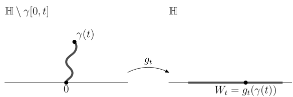
Figure 16: The mapping $g_{t}$ maps the complement of $\gamma[0,t]$ onto the upper half-plane. The tip $\gamma(t)$ is mapped to a point $W_{t}$ on the real line.

Consider more general families of growing sets. Call a compact subset $K$ of $\overline{\mathbb{H}}$ such that $\mathbb{H}\setminus K$ is simply connected, as a hull . The sets $K_{t}$ given by a simple curve, as above, are hulls. Also other families of hulls can be described by the Loewner equation with a continuous driving function. The necessary and sufficient condition is given in the following proposition. Also some facts about the capacity are collected there.

Proposition A.1.

Let $T>0$ and $(K_{t})_{t\in[0,T]}$ a family of hulls s.t. $K_{s}\subset K_{t}$, for any $s<t$, and let $H_{t}=\mathbb{H}\setminus K_{t}$.

• If $(K_{t}\setminus K_{s})\cap\mathbb{H}\neq\emptyset$ for all $s<t$, then $t\mapsto\mathrm{cap}_{\mathbb{H}}(K_{t})$ is strictly increasing

• If $t\mapsto H_{t}$ is continuous in Carathéodory kernel convergence, then $t\mapsto\mathrm{cap}_{\mathbb{H}}(K_{t})$ is continuous.

• Assume that $\mathrm{cap}_{\mathbb{H}}(K_{t})=2t$ (under the first two assumptions there is always such a time reparameterization). Then there is a continuous driving function $W_{t}$ so that $g_{t}$ satisfies Loewner equation (106) if and only if for each $\delta>0$ there exists $\varepsilon>0$ so that for any $0\leq s<t\leq T$, $|t-s|<\delta$, a connected set $C\subset H_{s}$ can be chosen such that $\operatorname{diam}(C)<\varepsilon$ and $C$ separates $K_{t}\setminus K_{s}$ from infinity.

Two first statements are relatively simple. The second claim is almost self-evident: Carathéodory kernel convergence means that $g_{s}\to g_{t}$ as $s\to t$ in the compact subsets of $H_{t}$ and then we have to use the fact that $\mathrm{cap}_{\mathbb{H}}(K)$ can be expressed as an integral $\frac{1}{2\pi}\int_{0}^{\pi}\operatorname{Re}\big{(}Re^{i\theta}g_{K}(Re^{i\theta})\big{)}\mathrm{d}\theta$ for $R$ large enough. The third claim is proved in [21].

By the third claim not all continuous $W_{t}$ correspond to a simple curve. One important class of $(K_{t})_{t\in[0,T]}$ are the ones generated by a curve in the following sense: For a curve $\gamma:[0,T]\to\overline{\mathbb{H}}$, $\gamma(0)\in\mathbb{R}$, that is not necessarily simple, define $H_{t}$ to be the unbounded component of $\mathbb{H}\setminus\gamma[0,t]$ and $K_{t}=\overline{\mathbb{H}\setminus H_{t}}$. For each $t$, $K_{t}$ is a hull and the collection of hulls $(K_{t})_{t\in[0,T]}$ is said to be generated by the curve $\gamma$. But even this class is not general enough: a counterexample is a spiral that winds infinitely many times around a circle in the upper half-plane and then unwinds, see for example the discussion in the article by Lind, Marshall and Rohde [23].

A Schramm–Loewner evolution, SLE_κ, $\kappa>0$, is a random $(K_{t})_{t\geq 0}$ corresponding to a random driving function $W_{t}=\sqrt{\kappa}B_{t}$ where $(B_{t})_{t\geq 0}$ is a standard one-dimensional Brownian motion. SLE was introduced by Schramm [28] in 1999. An important result about them is that they are curves in the following sense:

• $0<\kappa\leq 4$: $K_{t}$ is a simple curve

• $4<\kappa<8$: $K_{t}$ is generated by a curve

• $\kappa\geq 8$: $K_{t}$ is a space filling curve

This is proven $\kappa\neq 8$ in [27]. For $\kappa=8$, it follows since SLE₈ is a scaling limit of a random planar curve in the sense explained in the current paper, see [22]. So based on this result, the above definition can be reformulated: a Schramm–Loewner evolution is a random curve in the upper half-plane whose Loewner evolution is driven by a Brownian motion.

In fact, Schramm–Loewner evolutions are characterized by the conformal Markov property [28], see [35] for an extended discussion. For this reason, if the scaling limit of a random planar curve is conformally invariant in an appropriate sense, then it has to be SLE_κ, for some $\kappa>0$.

A.2 Equicontinuity of Loewner chains

In this section, we prove simple statements about equicontinuity of general Loewner chains. For $g_{t}$ as in the previous section, denote its inverse by $f_{t}=g_{t}^{-1}$, which satisfies the corresponding Loewner equation

$$\partial_{t}f_{t}(z)=-f_{t}^{\prime}(z)\frac{2}{z-W_{t}}$$ (107)

together with the initial condition $f_{0}(z)=z$. We call any of the equivalent objects $(g_{t})_{t\in[0,T]}$, $(f_{t})_{t\in[0,T]}$ and $(K_{t})_{t\in[0,T]}$ as a Loewner chain (with the driving term $(W_{t})_{t\in[0,T]}$).

Let $V_{T,\delta}=[0,T]\times\{z\in\mathbb{C}\,:\,\operatorname{Im}z\geq\delta\}$

Lemma A.2.

For any $T,\delta>0$ the family

$$\left\{\tilde{F}:V_{T,\delta}\to\mathbb{C}\,:\,\begin{gathered}\text{there is a Loewner chain $(f_{t})_{t\in\mathbb{R}_{+}}$ s.t. }\\ \tilde{F}(t,z)=f_{t}(z),\,\forall(t,z)\in V_{T,\delta}\end{gathered}\right\}$$ (108)

is equicontinuous and

$$\left|\partial_{t}\tilde{F}(t,z)\right|\leq\frac{2}{\delta}e^{8\frac{t}{\delta^{2}}},\qquad\left|\partial_{z}\tilde{F}(t,z)\right|\leq e^{8\frac{t}{\delta^{2}}}$$ (109)

for any $\tilde{F}$ in the set (108) and for any $(t,z)\in V_{T,\delta}$.

Proof.

Since $V_{T,\delta}$ is convex, it is sufficient to show (109). The equicontinuity follows from that bound by integrating along a line segment in $V_{T,\delta}$

Let $\Phi_{w}(z)=i(\operatorname{Im}w)\frac{1+z}{1-z}+\operatorname{Re}w$ and $f:\mathbb{H}\to\mathbb{C}$ be any conformal map. Then

$$z\mapsto\frac{f\circ\Phi_{w}(z)-f\circ\Phi_{w}(0)}{\Phi_{w}^{\prime}(0)f^{\prime}(w)}$$

belongs to the class $S$ of univalent functions, see Chapter 2 of [13], and therefore by Bieberbach’s theorem

$$(\operatorname{Im}w)\left|\frac{f^{\prime\prime}(w)}{f^{\prime}(w)}\right|\leq 3.$$

If we apply this bound to the Loewner equation of $f^{\prime}_{t}$ we find that

$$|\partial_{t}f_{t}^{\prime}(z)|\leq\frac{8}{(\operatorname{Im}z)^{2}}|f_{t}^{\prime}(z)|$$

and therefore

$$|f_{t}^{\prime}(z)|\leq e^{8\frac{t}{(\operatorname{Im}z)^{2}}}\leq e^{8\frac{T}{\delta^{2}}}.$$

Furthermore, plugging this estimate in the Loewner equation gives

$$|\partial_{t}f_{t}(z)|\leq\frac{2}{\operatorname{Im}z}e^{8\frac{T}{\delta^{2}}}\leq\frac{2}{\delta}e^{8\frac{T}{\delta^{2}}}.$$

∎

For $T,\delta>0$ and family of hulls $(K_{t})_{t\in[0,T]}$, let

$$S_{K}(T,\delta)=\{(t,z)\in[0,T]\times\overline{\mathbb{H}}\,:\,\operatorname{dist}(z,K_{t})\geq\delta\}$$ (110)

Lemma A.3.

Let $\gamma_{n}$ be a sequence of curves in $\mathbb{H}$ and let $\gamma$ be a curve in $\mathbb{H}$ all parametrized with the interval $[0,T]$, $T>0$, and let $g_{n,t}$ and $g_{t}$ be the normalized conformal maps related to the hulls $K_{n,t}$ and $K_{t}$ of $\gamma_{n}[0,t]$ and $\gamma[0,t]$, respectively. If $\gamma_{n}\to\gamma$ uniformly, then $g_{n,t}\to g_{t}$ uniformly on $S_{K}(T,\delta)$. Especially $\mathrm{cap}_{\mathbb{H}}\gamma_{n}[0,\cdot]\to\mathrm{cap}_{\mathbb{H}}\gamma[0,\cdot]$ uniformly.

Proof.

The lemma follows from the Carathéodory convergence theorem (Theorem 3.1 of [13] and Theorem 1.8 of [26]). Convergence is uniform in $t$ since the interval $[0,T]$ is compact. ∎

Lemma A.4.

Let $W_{n}$ be a sequence of continuous functions on $[0,T]$ and let $W$ be a continuous functions on $[0,T]$ and let $g_{n,t}$ and $g_{t}$ be the solutions of Loewner equation with the driving terms $W_{n,t}$ and $W_{t}$, respectively, and let $K_{t}$ be the hull of $g_{t}$. If $W_{n}\to W$ uniformly, then $g_{n,t}\to g_{t}$ uniformly on $S_{K}(T,\delta)$ and $g_{t}$ and $W$ satisfy the Loewner equation.

Proof.

This lemma follows from the basic properties of ordinary differential equations. ∎

A.2.1 Main lemma

Consider a sequence $\tilde{\gamma}_{n}\in X_{\mathrm{simple}}(\mathbb{D})$ with $\tilde{\gamma}_{n}(0)=-1$ and $\tilde{\gamma}_{n}(1)=+1$ which converges to some curve $\tilde{\gamma}\in X$. After choosing a parametrization and using the chosen conformal transformation from $\mathbb{D}$ to $\mathbb{H}$, it is natural to consider for some $T>0$ a sequence of one-to-one continuous functions $\gamma_{n}:[0,T]\to\mathbb{C}$ with $\gamma_{n}(0)\in\mathbb{R}$ and $\gamma(0,T]\subset\mathbb{H}$ such that $\gamma_{n}$ converges uniformly to a continuous function $\gamma:[0,T]\to\mathbb{C}$ which is not constant on any subinterval of $[0,T]$. In this section we present practical conditions under which $\gamma$ is a Loewner chain, that is, $\gamma$ can be reparametrized with the half-plane capacity.

Let

$$\upsilon_{n}(t)=\frac{1}{2}\mathrm{cap}_{\mathbb{H}}(\gamma_{n}[0,t]),\qquad\upsilon(t)=\frac{1}{2}\mathrm{cap}_{\mathbb{H}}(\gamma[0,t]).$$ (111)

Then $t\mapsto\upsilon_{n}(t)$ and $t\mapsto\upsilon(t)$ are continuous and $\upsilon_{n}\to\upsilon$ uniformly as $n\to\infty$. In particular, $\lim_{n}\upsilon_{n}(T)=\upsilon(T)$ and by the assumptions $\upsilon(1)>0$. Furthermore, $t\mapsto\upsilon(t)$ is non-decreasing. Let $(W_{n}(t))_{t\in[0,\upsilon_{n}(T)]}$ be the driving term of $\gamma_{n}$ which exists since $\gamma_{n}$ is simple.

When is it true that $\gamma$ has a continuous driving term? It is a fact that if $\upsilon$ is strictly increasing then $\gamma$ has a driving term $W((t))_{t\in[0,\upsilon(1)]}$ and that $W_{n}\to W$ uniformly on $[0,\upsilon(1))$. However we won’t prove this auxiliary result, instead we prove a weaker result which gives a practical conditions to be verified.

Lemma A.5.

Let $T>0$ and for each $n\in\mathbb{N}$, let $\gamma_{n}:[0,T]\to\mathbb{C}$ be injective continuous function such that $\gamma_{n}(0)\in\mathbb{R}$ and $\gamma_{n}(0,T]\subset\mathbb{H}$. Suppose that

1. $\gamma_{n}\to\gamma$ uniformly on $[0,T]$ and $\gamma$ is not constant on any subinterval of $[0,T]$

2. $W_{n}\to W$ uniformly on $[0,\upsilon(T)]$.

3. $F_{n}\to F$ uniformly on $[0,T]\times[0,1]$, where

   $$F_{n}(t,y)=g_{\gamma_{n}[0,t]}^{-1}\big{(}\,W_{n}(\upsilon_{n}(t))+iy\,\big{)}.$$ (112)

Then $t\mapsto\upsilon(t)$ is strictly increasing and $g_{t}\mathrel{\mathop{:}}=g_{\gamma\circ\upsilon^{-1}[0,t]}$ satisfies the Loewner equation with the driving term $W$. Furthermore, $\gamma_{n}\circ\upsilon_{n}^{-1}$, which is the sequence of curves in the capacity parametrization, converges uniformly to $\gamma\circ\upsilon^{-1}$ and the sequence of mappings $(t,z)\mapsto g_{\gamma_{n}\circ\upsilon_{n}^{-1}[0,t]}(z)$ converges to $g_{t}$ uniformly on

$$S_{K}(T,\delta)=\{(t,z)\in[0,T]\times\overline{\mathbb{H}}\,:\,\operatorname{dist}(z,K_{t})\geq\delta\}$$ (113)

for any $\delta>0$. Here $K_{t}$ is the hull of $\gamma[0,t]$.

Remark A.6.

By applying a scaling and corresponding time change, it’s enough that there exists $\varepsilon>0$ such that $F_{n}\to F$ uniformly on $[0,T]\times[0,\varepsilon]$.

Proof.

By Lemma A.3, $\gamma_{n}\to\gamma$ implies that $\upsilon_{n}\to\upsilon$ uniformly as $n\to\infty$. Let $f_{n,t}=g_{\gamma_{n}[0,t]}^{-1}$. Since

$$F_{n}(t,y)=f_{n,t}(W_{n}\circ\upsilon_{n}(t)+i\,y)$$ (114)

and since by Lemma A.2

$$|f_{n,t}(z)-f_{n,t^{\prime}}(z^{\prime})|\leq C(\delta,\upsilon(T))\,\left(|\upsilon_{n}(t)-\upsilon_{n}(t^{\prime})|+|z-z^{\prime}|\right),$$ (115)

it follows directly from the assumptions that if for some $s<t$, $\upsilon(s)=\upsilon(t)$, then $F(s,y)=F(u,y)=F(t,y)$ for all $u\in[s,t]$ and $y\geq 0$. Especially $\gamma(u)=F(u,0)$ is constant on the interval $u\in[s,t]$ which contradicts with the assumptions of the lemma. Hence $\upsilon$ is strictly increasing. An application of Helly’s selection theorem gives that $\upsilon_{n}^{-1}$ converges uniformly to $\upsilon^{-1}$. Therefore $\gamma_{n}\circ\upsilon_{n}^{-1}$ converges uniformly to $\gamma\circ\upsilon^{-1}$ and hence for any $\delta>0$ $(t,z)\mapsto g_{\gamma_{n}\circ\upsilon_{n}^{-1}[0,t]}$ converges to $g_{t}$ uniformly on the set (113). The convergence of $W_{n}$ together with standard results about ODE’s imply that $g_{\gamma_{n}\circ\upsilon_{n}^{-1}[0,t]}$, which are the solutions of the Loewner equation with the driving terms $W_{n}$, converge uniformly to the solution of the Loewner equation with the driving term $W$, see Lemma A.4. Hence $g_{t}$ is generated by $\gamma$ and driven by $W$. ∎

Lemma A.7.

Let $\gamma:[0,T]\to\mathbb{C}$ be continuous and not constant on any subinterval of $[0,T]$. Let $\gamma_{n}:[0,T]\to\mathbb{C}$ be a sequence of simple parametrized curves such that $\gamma_{n}(0)\in\mathbb{R}$ and $\gamma_{n}(\,(0,T]\,)\subset\mathbb{H}$. Suppose that $\gamma_{n}\to\gamma$ uniformly as $n\to\infty$. If

• $(W_{n})_{n\in\mathbb{N}}$ is equicontinuous and

• there exist increasing continuous $\psi:[0,\delta)\to\mathbb{R}_{+}$ such that $\psi(0)=0$ and $|F_{n}(t,y)-\gamma_{n}(t)|\leq\psi(y)$ for all $0<y<\delta$ and for all $n\in\mathbb{N}$

then $W_{n}$ converges to some continuous $W$, $\gamma$ can be continuously reparametrized with the half-plane capacity and $\gamma\circ\upsilon^{-1}$ is driven by $W$.

Proof.

It is clearly enough to show that $(F_{n})_{n\in\mathbb{N}}$ is a equicontinuous family of functions on $[0,T]\times[0,1]$. The claim then follows from the previous lemma after choosing by Arzelà-Ascoli theorem a subsequence $n_{j}$ such that $F_{n_{j}}$ and $W_{n_{j}}$ converge.

Let $g_{n,t}=g_{\gamma_{n}[0,t]}$ and $f_{n,t}=g_{n,t}^{-1}$. Let $\varepsilon>0$ and choose $\delta>0$ such that

$$|F_{n}(t,y)-\gamma_{n}(t)| \leq\frac{\varepsilon}{6}$$ (116)

$$|\gamma_{n}(t^{\prime})-\gamma_{n}(t)| \leq\frac{\varepsilon}{6}$$ (117)

when $0\leq y\leq\delta$ and $t,t^{\prime}\in[0,T]$ with $|t-t^{\prime}|\leq\delta$. Then by the triangle inequality

$$|F_{n}(t^{\prime},y^{\prime})-F_{n}(t,y)|\leq\frac{\varepsilon}{2}$$ (118)

for all $0\leq y,y^{\prime}\leq\delta$, for all $t,t^{\prime}\in[0,T]$ with $|t-t^{\prime}|\leq\delta$ and for all $n\in\mathbb{N}$.

By (114) and Lemma A.2, the family of mappings $(F_{n}|_{[0,T]\times[\delta,1]})_{n\in\mathbb{N}}$ is equicontinuous. Hence we can choose $0<\tilde{\delta}\leq\delta$ such that (118) for all $\delta\leq y,y^{\prime}\leq 1$ with $|y-y^{\prime}|\leq\tilde{\delta}$, for all $t,t^{\prime}\in[0,T]$ with $|t-t^{\prime}|\leq\tilde{\delta}$ and for all $n\in\mathbb{N}$. Hence by the triangle inequality

$$|F_{n}(t^{\prime},y^{\prime})-F_{n}(t,y)|\leq\varepsilon$$ (119)

for all $0\leq y,y^{\prime}\leq 1$ with $|y-y^{\prime}|\leq\tilde{\delta}$, for all $t,t^{\prime}\in[0,T]$ with $|t-t^{\prime}|\leq\tilde{\delta}$ and for all $n\in\mathbb{N}$. ∎

A.3 Some facts about conformal mappings

In this section, a collection of simple lemmas about normalized conformal mappings is presented. Only elementary methods are used, and therefore it is advantageous to present the proofs here, even though they appear elsewhere in the literature.

Denote the inverse mapping of $g_{K}$ by $f_{K}$ and by $I\subset\mathbb{R}$ the image of $\partial K$ under $g_{K}$, i.e. $I=\overline{\{x\in\mathbb{R}\,:\,\operatorname{Im}f_{K}(x)>0\}}$. Now $f_{K}$ can be given by integral with Poisson kernel of upper half-plane as

$$f_{K}(z)=z+\frac{1}{\pi}\int_{I}\frac{\operatorname{Im}f_{K}(x)}{x-z}\mathrm{d}x.$$ (120)

This gives a nice proof of the following fact.

Lemma A.8.

Denote $u_{+}=\max I$ and $u_{-}=\min I$ and $x_{\pm}=f_{K}(u_{\pm})$. Assume $\mathbb{H}\cap K\neq\emptyset$. Then

$$f_{K}(x)<x\textrm{ when }x\geq u_{+}\textrm{ and }f_{K}(x)>x\textrm{ when }x\leq u_{-}$$ (121)

and

$$g_{K}(x)>x\textrm{ when }x\geq x_{+}\textrm{ and }g_{K}(x)<x\textrm{ when }x\leq x_{-}.$$ (122)

Proof.

Note that $\operatorname{Im}f_{K}(x)$ is non-negative everywhere. It is positive in a set of non-zero Lebesgue measure, otherwise the equation (120) would imply that $f_{K}$ is an identity which is a contradiction. Now the equation (120) implies directly the equation (121). Apply $g_{K}$ on both sides to get the equation (122). ∎

The lemma can be used, for example, in the following way.

Lemma A.9.

Let $K\subset K^{\prime}$ be two hulls. Let $x\in\mathbb{R}$ s.t. $g_{K}(\overline{K^{\prime}\setminus K})\cap(x,\infty)=\emptyset$, and let $z=f_{K}(x)$. Then $g_{K}(z)\leq g_{K^{\prime}}(z)$.

Proof.

Apply Lemma A.8 to hull $J=g_{K}(\overline{K^{\prime}\setminus K})$ and $u=g_{J}(x)$. ∎

Let’s introduce still one more concept. Consider now $K=[-l,l]\times[0,h]$ where $l,h>0$. The domain $\mathbb{H}\setminus K$ can be thought as a polygon with the vertices $w_{1}=-l$, $w_{2}=-l+ih$, $w_{3}=l+ih$, $w_{4}=l$ and $w_{5}=\infty$. The interior angles at these vertices are $\alpha_{1}=\frac{\pi}{2}$, $\alpha_{2}=\frac{3\pi}{2}$, $\alpha_{3}=\frac{3\pi}{2}$, $\alpha_{4}=\frac{\pi}{2}$ and $\alpha_{5}=0$, respectively. For the last one, this has to be thought on the Riemann sphere.

Mappings from $\mathbb{H}$ to polygons are well-known. They are Schwarz-Christoffel mappings. In this case, when $f_{K}(\infty)=w_{5}=\infty$ all such mappings can be written in the form

$$f_{K}(z)=A+C\int^{z}\frac{\sqrt{\zeta-z_{2}}\sqrt{\zeta-z_{3}}}{\sqrt{\zeta-z_{1}}\sqrt{\zeta-z_{4}}}\mathrm{d}\zeta.$$ (123)

Here $f_{K}(z_{i})=w_{i}$, $i=1,2,3,4$. So in a sense $\operatorname{Re}A,\operatorname{Im}A,C$ and $z_{i}$ are parameters in the problem. Two of them can be chosen freely and the rest are determined from them. The branches of the square roots are chosen so that far on the positive real axis the square root is positive and then analytic continuation is used.

In our case $f_{K}$ is normalized at the infinity. This fixes $C=1$ and $\operatorname{Re}A$ so that it cancels the constant term in the expansion of the integral. But if we are only interested in differences $f_{K}(z)-f_{K}(z^{\prime})$ we don’t have to care about $A$.

Lemma A.10.

Let $K=[-l/2,l/2]\times[0,h]$, $h,l>0$, and let $z_{i}$ be as above. Then

$$z_{3}=-z_{2}=\frac{1}{2}l\,\big{(}1+o(1)\big{)}\textrm{ and }z_{4}-z_{3}=z_{2}-z_{1}=\frac{2}{\pi}h\,\big{(}1+o(1)\big{)}\textrm{ as }\frac{h}{l}\to 0.$$ (124)

Proof.

Note first that by symmetry $z_{1}=-z_{4}$ and $z_{2}=-z_{4}$.

Denote $\lambda=z_{3}-z_{2}$ and $\theta=z_{4}-z_{3}$. We would like to estimate $\lambda$ and $\theta$ in terms of $l$ and $h$.

Calculate $h=\operatorname{Im}(w_{3}-w_{4})$ as an integral along the real axis

$$h=\int_{z_{3}}^{z_{4}}\sqrt{\frac{\zeta-z_{2}}{\zeta-z_{1}}}\sqrt{\frac{\zeta-z_{3}}{z_{4}-\zeta}}\mathrm{d}\zeta.$$

Since the first factor of the integrand is a decreasing function $\zeta$, it can be bounded with the values at the end points $z_{3}$ and $z_{4}$. After couple of variable changes, the integral of the second factor is

$$\int_{z_{3}}^{z_{4}}\sqrt{\frac{\zeta-z_{3}}{z_{4}-\zeta}}\mathrm{d}\zeta=\frac{\pi}{2}(z_{4}-z_{3})$$

and therefore

$$\frac{\pi}{2}\sqrt{\frac{1}{1+\frac{\theta}{\lambda}}}\,\theta\leq h\leq\frac{\pi}{2}\sqrt{\frac{1+\frac{\theta}{\lambda}}{1+2\frac{\theta}{\lambda}}}\,\theta.$$ (125)

Calculate $l=w_{3}-w_{2}$ as

$$l=\int_{z_{2}}^{z_{3}}\sqrt{\frac{(\zeta-z_{2})(z_{3}-\zeta)}{(\zeta-z_{1})(z_{4}-\zeta)}}\mathrm{d}\zeta=2\int_{0}^{z_{3}}\sqrt{\frac{z_{3}^{2}-\zeta^{2}}{z_{4}^{2}-\zeta^{2}}}\mathrm{d}\zeta$$

The integrand is always less or equal then one. So $l\leq\lambda$. For the lower bound, note that the integrand is a decreasing function of $\zeta$. Therefore

$$\int_{0}^{z_{3}}\sqrt{\frac{z_{3}^{2}-\zeta^{2}}{z_{4}^{2}-\zeta^{2}}}\mathrm{d}\zeta\geq\zeta_{0}\sqrt{\frac{z_{3}^{2}-\zeta_{0}^{2}}{z_{4}^{2}-\zeta_{0}^{2}}}$$

Maximize this with respect to $\zeta_{0}\in[0,z_{3}]$ to get

$$\int_{0}^{z_{3}}\sqrt{\frac{z_{3}^{2}-\zeta^{2}}{z_{4}^{2}-\zeta^{2}}}\mathrm{d}\zeta\geq\left(z_{4}-\sqrt{z_{4}^{2}-z_{3}^{2}}\right)$$

To conclude this

$$\left(1+2\frac{\theta}{\lambda}-2\sqrt{\frac{\theta}{\lambda}}\sqrt{1+\frac{\theta}{\lambda}}\right)\,\lambda\leq l\leq\lambda$$ (126)

The inequalities (125) and (126) can be combined to conclude that $\frac{\theta}{\lambda}$ is small when $\frac{h}{l}$ is small. And in this case $\theta\approx\frac{2}{\pi}h$ and $\lambda\approx l$. And all the claims follow. ∎

Lemma A.11.

Let hull $K$ be a subset of a rectangle $[-l,l]\times[0,h]$, $l,h>0$. If $K\cap\,(\{l\}\times[0,h])\neq\emptyset$ then uniformly for any $z$ in this set $g_{K}(z)=l\big{(}1+o(1)\big{)}$ as $\frac{h}{l}\to 0$.

Proof.

Assume that $K\cap\mathbb{H}\neq\emptyset$. Otherwise the statement is trivial since $z=l$ and $g_{K}$ is identity.

Let $K^{\prime}=[-l,l]\times[0,h]$. Then $K\subset K^{\prime}$. Take any $z\in K\cap\,(\{l\}\times[0,h])$. Let $x_{+}=l$, $u_{+}=g_{K}(x_{+})$ and $v_{+}=g_{K^{\prime}}(x_{+})$.

By Lemma A.9 and Lemma A.10 $l\leq u_{+}\leq v_{+}=l\big{(}1+o(1)\big{)}$. And by an length area principle, for example, Wolff’s lemma (Proposition 2.2 of [26]), $0\leq u_{+}-g_{K}(z)=o(1)\,l$.∎

Lemma A.12.

If $i\in K$ then $\mathrm{cap}_{\mathbb{H}}(K)\geq\frac{1}{4}$.

Proof.

First of all note that this is sharp. It is attained by a vertical slit extending from $0$ to $i$.

Now assume that there is $K$ containing $i$ s.t. $\mathrm{cap}_{\mathbb{H}}(K)<\frac{1}{4}$. It is possible to choose $\tilde{K}$ containing $K$ s.t. the capacities are arbitrarily close and the boundary of $\tilde{K}$ is a smooth curve. This can be done by choosing a smooth, simple curve $\gamma$ that separates an interval containing $g_{K}(K)$ from $\infty$ in $\mathbb{H}$. Then $\tilde{K}$ is the hull that has $f_{K}(\gamma)$ as the boundary. Therefore there exists now $\tilde{K}$ s.t. it contains $i$, $\mathrm{cap}_{\mathbb{H}}(\tilde{K})<\frac{1}{4}$ and the boundary is a curve.

Therefore, there exists a simple curve $\gamma(t)$, $t\in[0,T]$, parameterized by the capacity so that $0<T<\frac{1}{4}$ and $\gamma$ contains some point lying on the line $i+\mathbb{R}$. Now take any point $z$ s.t. $\operatorname{Im}z>4T$, and let $Z_{t}=X_{t}+iY_{t}=g_{t}(z)$. Then by Loewner equation

$$\frac{\mathrm{d}Y_{t}}{\mathrm{d}t}=-\frac{2Y_{t}}{(X_{t}-U_{t})^{2}+Y_{t}^{2}}\geq-\frac{2}{Y_{t}}.$$

Therefore

$$Y_{t}\geq\sqrt{\big{(}\operatorname{Im}z\big{)}^{2}-4t}>0.$$

Hence $z\notin\gamma[0,T]$. This leads to a contradiction: $\gamma$ doesn’t intersect the line $i+\mathbb{R}$. ∎

Lemma A.13.

Let $K$ be a hull. If $K\cap\big{(}\mathbb{R}\times\{hi\}\big{)}\neq\emptyset$ then $\mathrm{cap}_{\mathbb{H}}(K)\geq\frac{1}{4}h^{2}$. If $K\subset[-l,l]\times[0,h]$, then $\mathrm{cap}_{\mathbb{H}}(K)\leq\mathrm{cap}_{\mathbb{H}}\big{(}[-l,l]\times[0,h]\big{)}$ and $\mathrm{cap}_{\mathbb{H}}\big{(}[-l,l]\times[0,h]\big{)}=\frac{1}{2\pi}hl\big{(}1+o(1)\big{)}$ as $\frac{h}{l}\to 0$.

Proof.

The lower bound follows from Lemma A.12 and scaling.

For the upper bound let’s use the Schwarz-Christoffel mapping. Write

$$\mathrm{cap}_{\mathbb{H}}(K) =\frac{1}{8}\big{(}-z_{1}^{2}-z_{4}^{2}+z_{2}^{2}+z_{3}^{2}\big{)}=\frac{1}{4}\big{(}z_{4}-z_{3}\big{)}\big{(}z_{4}+z_{3}\big{)}$$

$$=\frac{1}{2\pi}hl\big{(}1+o(1)\big{)}$$ (127)

This gives the desired upper bound. ∎

References

- [1] L. V. Ahlfors. Conformal invariants: topics in geometric function theory. McGraw-Hill Book Co., New York, 1973.
- [2] M. Aizenman and A. Burchard. Hölder regularity and dimension bounds for random curves. Duke Math. J., 99(3):419–453, 1999.
- [3] M. Aizenman, A. Burchard, C. M. Newman, and D. B. Wilson. Scaling limits for minimal and random spanning trees in two dimensions. Random Structures Algorithms, 15(3-4):319–367, 1999. Statistical physics methods in discrete probability, combinatorics, and theoretical computer science (Princeton, NJ, 1997).
- [4] V. Beffara and H. Duminil-Copin. The self-dual point of the two-dimensional random-cluster model is critical for . Probab. Theory Related Fields, 153(3-4):511–542, 2012.
- [5] P. Billingsley. Convergence of probability measures. Wiley Series in Probability and Statistics: Probability and Statistics. John Wiley & Sons Inc., New York, second edition, 1999. A Wiley-Interscience Publication.
- [6] F. Camia and C. M. Newman. Two-dimensional critical percolation: the full scaling limit. Comm. Math. Phys., 268(1):1–38, 2006.
- [7] F. Camia and C. M. Newman. Critical percolation exploration path and : a proof of convergence. Probab. Theory Related Fields, 139(3-4):473–519, 2007.
- [8] D. Chelkak. Robust Discrete Complex Analysis: A Toolbox. ArXiv e-prints, dec 2012, 1212.6205.
- [9] D. Chelkak, H. Duminil-Copin, and C. Hongler. Crossing probabilities in topological rectangles for the critical planar FK-Ising model. ArXiv e-prints, Dec. 2013, 1312.7785.
- [10] D. Chelkak, H. Duminil-Copin, C. Hongler, A. Kemppainen, and S. Smirnov. Convergence of Ising interfaces to Schramm’s SLE curves. C. R. Math. Acad. Sci. Paris, 352(2):157–161, 2014.
- [11] D. Chelkak and S. Smirnov. Universality in the 2D Ising model and conformal invariance of fermionic observables. Invent. Math., 189(3):515–580, 2012.
- [12] H. Duminil-Copin, V. Sidoravicius, and V. Tassion. Continuity of the phase transition for planar Potts models with . In preparation, 2014.
- [13] P. L. Duren. Univalent functions, volume 259 of Grundlehren der Mathematischen Wissenschaften [Fundamental Principles of Mathematical Sciences]. Springer-Verlag, New York, 1983.
- [14] R. Durrett. Probability: theory and examples. Duxbury Press, Belmont, CA, second edition, 1996.
- [15] G. Grimmett. The random-cluster model, volume 333 of Grundlehren der Mathematischen Wissenschaften [Fundamental Principles of Mathematical Sciences]. Springer-Verlag, Berlin, 2006.
- [16] G. Grimmett. Probability on graphs, volume 1 of Institute of Mathematical Statistics Textbooks. Cambridge University Press, Cambridge, 2010. Random processes on graphs and lattices.
- [17] F. Johansson Viklund, S. Rohde, and C. Wong. On the continuity of in . Probab. Theory Related Fields, 159(3-4):413–433, 2014.
- [18] A. Kemppainen. On convergence of uniform spanning tree interface to SLE(8). In preparation, 2015.
- [19] A. Kemppainen and S. Smirnov. Conformal invariance in random cluster models. II. Full scaling limit as a branching SLE. In preparation, 2015.
- [20] G. F. Lawler. Conformally invariant processes in the plane, volume 114 of Mathematical Surveys and Monographs. American Mathematical Society, Providence, RI, 2005.
- [21] G. F. Lawler, O. Schramm, and W. Werner. Values of Brownian intersection exponents. I. Half-plane exponents. Acta Math., 187(2):237–273, 2001.
- [22] G. F. Lawler, O. Schramm, and W. Werner. Conformal invariance of planar loop-erased random walks and uniform spanning trees. Ann. Probab., 32(1B):939–995, 2004.
- [23] J. Lind, D. E. Marshall, and S. Rohde. Collisions and spirals of Loewner traces. Duke Math. J., 154(3):527–573, 2010.
- [24] K. Löwner. Untersuchungen über schlichte konforme Abbildungen des Einheitskreises. I. Math. Ann., 89(1-2):103–121, 1923.
- [25] N. Makarov and S. Smirnov. Off-critical lattice models and massive SLEs. In XVIth International Congress on Mathematical Physics, pages 362–371. World Sci. Publ., Hackensack, NJ, 2010.
- [26] C. Pommerenke. Boundary behaviour of conformal maps, volume 299 of Grundlehren der Mathematischen Wissenschaften. Springer-Verlag, Berlin, 1992.
- [27] S. Rohde and O. Schramm. Basic properties of SLE. Ann. of Math. (2), 161(2):883–924, 2005.
- [28] O. Schramm. Scaling limits of loop-erased random walks and uniform spanning trees. Israel J. Math., 118:221–288, 2000.
- [29] O. Schramm and S. Sheffield. Harmonic explorer and its convergence to . Ann. Probab., 33(6):2127–2148, 2005.
- [30] O. Schramm and S. Sheffield. Contour lines of the two-dimensional discrete Gaussian free field. Acta Math., 202(1):21–137, 2009.
- [31] S. Sheffield. Exploration trees and conformal loop ensembles. Duke Math. J., 147(1):79–129, 2009.
- [32] S. Sheffield and N. Sun. Strong path convergence from Loewner driving function convergence. Ann. Probab., 40(2):578–610, 2012.
- [33] S. Smirnov. Critical percolation in the plane: conformal invariance, Cardy’s formula, scaling limits. C. R. Acad. Sci. Paris Sér. I Math., 333(3):239–244, 2001.
- [34] S. Smirnov. Critical percolation and conformal invariance. In XIVth International Congress on Mathematical Physics, pages 99–112. World Sci. Publ., Hackensack, NJ, 2005.
- [35] S. Smirnov. Towards conformal invariance of 2D lattice models. In International Congress of Mathematicians. Vol. II, pages 1421–1451. Eur. Math. Soc., Zürich, 2006.
- [36] S. Smirnov. Critical percolation in the plane (long version). ArXiv e-prints, sep 2009, 0909.4499.
- [37] S. Smirnov. Conformal invariance in random cluster models. I. Holomorphic fermions in the Ising model. Ann. of Math. (2), 172(2):1435–1467, 2010.
- [38] D. Zhan. The scaling limits of planar LERW in finitely connected domains. Ann. Probab., 36(2):467–529, 2008.