Efficient high-dimensional entanglement imaging with a compressive sensing, double-pixel camera

Abstract

We implement a double-pixel, compressive sensing camera to efficiently characterize, at high resolution, the spatially entangled fields produced by spontaneous parametric downconversion. This technique leverages sparsity in spatial correlations between entangled photons to improve acquisition times over raster-scanning by a scaling factor up to $n^{2}/\log(n)$ for $n$-dimensional images. We image at resolutions up to $1024$ dimensions per detector and demonstrate a channel capacity of $8.4$ bits per photon. By comparing the entangled photons’ classical mutual information in conjugate bases, we violate an entropic Einstein-Podolsky-Rosen separability criterion for all measured resolutions. More broadly, our result indicates compressive sensing can be especially effective for higher-order measurements on correlated systems.

I Introduction

Spatially entangled biphotons, such as those generated by spontaneous parametric downconversion (SPDC), exhibit strong Einstein-Podolsky-Rosen (EPR) type correlations Einstein et al. (1935) in the transverse position and transverse momentum degrees of freedom Howell et al. (2004). Because these variables are continuous, the entanglement can be very high-dimensional with a typical Schmidt number greatly exceeding $1000$ Pors (2011). This provides high information density which can be leveraged to increase channel capacity and security for quantum key distribution Ekert (1991); Walborn et al. (2006, 2008) and dense coding Bennett and Wiesner (1992); Braunstein and Kimble (2000). Other applications include ghost imaging Pittman et al. (1995); Abouraddy et al. (2001), quantum computing Tasca et al. (2011), and quantum teleportation Walborn et al. (2007).

Experimentally characterizing the SPDC state is unfortunately difficult due to weak sources and low resolution detectors. Spatial entanglement is traditionally imaged by jointly raster-scanning photon-counting avalanche photodiodes (APDs) to measure spatial correlations. This scales extremely poorly with increasing detector resolution. With a biphoton flux of $4,000$ coincident detections per second, it would take $55$ days to jointly scan a $24\times 24$ pixel region for a signal-to-noise ratio (SNR) of $10$. For $32\times 32$ pixels, it would take $310$ days (see Eq. 9).

Other approaches have been tried with mixed success. Intensified CCD cameras can measure the Schmidt number Di Lorenzo Pires et al. (2009), but do not detect single-photon correlations rendering them ineffective for most quantum applications. Arrays of photon counting APDs could replace CCDs, but they are currently low resolution, noisy and resource intensive; especially since each pixel pair must be individually correlated Coffey (2011); Albota (2002); Itzler et al. (2010). A recent, promising result averages intensity correlations over many images from a single-photon sensitive electron-multiplying CCD, reporting $2500$ modes Edgar et al. (2012). This technique is limited to a $30$ ms exposure time (APDs are sub-ns) and is noisier than using APDs because it does not isolate individual coincident detections.

In ref Dixon et al. (2012), Dixon et. al. reduce the number of measurements required for a raster-scan by only measuring in an area of interest where correlations are expected, reporting a channel capacity of $7$ bits per photon. While not a true full-field measurement, they highlight a critical feature of the SPDC field. In both position and momentum representations, the distribution of correlations between pairs of detector pixels is very sparse despite dense (not sparse) single-particle distributions. Applying ideas from the field of compressive sensing, we exploit prior knowledge of this sparsity to beat the “curse of dimensionality” Bellman (2003) and efficiently characterize the full biphoton field without raster scanning.

In this article, we implement a compressive sensing, photon-counting double-pixel camera that efficiently images single-photon SPDC correlations in the near- and far-field at resolutions up to $32\times 32=1024$ dimensions per detector. At $32\times 32$ resolution, the measurement time is reduced from $310$ days for raster scanning to around $8$ hours. We perform an entropic characterization showing channel capacities of up to $8.4$ bits per photon, equivalent to $337$ independent, identically distributed modes. Sums of channel capacities in conjugate bases violate a EPR steering bound Schneeloch et al. (2012) by up to $6.6$ bits.

II Theory

II.1 Compressive Sensing

Compressive sensing is a technique that employs optimization to measure a sparsely represented $N$-dimensional signal from $M<N$ incoherent measurements Donoho (2006); Candes and Romberg (2007); Baraniuk (2007); Candes and Wakin (2008). The approach is so-named because the signal is effectively compressed during measurement. Though sparsity is assumed, it is not known prior to measurement which elements contain appreciable amplitude. Compressive sensing must determine both which elements are significant and find their values.

To detect a sparsely represented $N$-dimensional signal vector $X$, we measure a series of $M<N$ values $Y$ by multiplying $X$ by an $M\times N$ sensing matrix $A$ such that

$$Y=\bm{AX}+\bm{\Gamma},$$ (1)

where $\Gamma$ is a noise vector.

Because $M<N$, this system is undetermined; a given $Y$ does not specify a unique $X$. The correct $X$ is recovered by minimizing a regularized least squares objective function

$$\min_{X}\frac{1}{2}||Y-AX||^{2}_{2}+\tau g(X),$$ (2)

where for example $||\Omega||^{2}_{2}$ is the $\ell_{2}$ norm of $\Omega$ and $\tau$ is a scaling constant. The function $g(X)$ is a regularization promoting sparsity. Common $g(X)$ include $X$’s $\ell_{1}$ norm, assuming the signal is sparse, and $X$’s total variation, assuming the signal’s gradient is sparse Candes and Romberg (2005). $A$ must be incoherent with the basis of interest, with the surprising and non-intuitive result that a random, binary sensing matrix works well. Given sufficiently large $M$, the recovered $X$ approaches the exact signal with high probability Candes et al. (2006). For a $k-$sparse signal, the required $M$ scales as $M\propto k\log(N/k)$.

Incoherent, random sampling is particularly beneficial for low-light measurements as each measurement receives on average half the total photon flux $\Phi/2$, as apposed to $\Phi/n$ for a raster scan. Compressive sensing is now beginning to be used for quantum applications such as state tomography Gross et al. (2010). Shabani et. al, for example, perform a tomography on a two qubit photonic gate for polarization entangled photons Shabani et al. (2011). CS has also been used to with spatially correlated light for ghost imaging Katz et al. (2009); Zerom et al. (2011). It is important to note that for ghost imaging, CS is not required to recover the full two-particle probability distribution as in entanglement characterization.

The quintessential compressed sensing example is the single-pixel camera Wakin et al. (2006); Duarte et al. (2008). An object is imaged onto a Digital Micromirror device (DMD), a 2D binary array of individually-addressable mirrors that reflect light either to a single detector or a dump. Rows of the sensing matrix $A$ consist of random, binary patterns placed sequentially on the DMD. For an $N$-dimensional image, minimizing Eq. 2 recovers images using as few as $M=0.02N$ measurements.

II.2 Compressive Sensing for Measuring Correlations

The single-pixel camera concept naturally adapts to imaging correlations by adding a second detector. Consider placing separate DMDs in the near-field or far-field of the SPDC signal and idler modes, where “on” pixels are redirected to photon counting modules. The signal of interest is

$$p_{x}(u,v) =\int\limits_{u}\mathrm{d}\vec{x_{s}}\int\limits_{v}\mathrm{d}\vec{x_{i}}|f(\vec{x_{s}},\vec{x_{i}})|^{2}$$ (3)

$$p_{k}(u,v) =\int\limits_{u}\mathrm{d}\vec{k_{s}}\int\limits_{v}\mathrm{d}\vec{k_{i}}|f(\vec{k_{s}},\vec{k_{i}})|^{2},$$ (4)

where $p(u,v)$ represents the probability of a coincident detection between the $u^{\text{th}}$ pixel on the signal DMD and $v^{\text{th}}$ pixel on the idler DMD. The functions $f(\vec{x_{s}},\vec{x_{i}})$ and $f(\vec{k_{s}},\vec{k_{i}})$ are approximate position and momentum wavefunctions for the biphoton

$$\psi(\vec{x_{s}},\vec{x_{i}})= \mathcal{N}\exp\left(-\frac{(\vec{x_{s}}-\vec{x_{i}})^{2}}{4\sigma_{c}^{2}}\right)\exp\left(-\frac{(\vec{x_{s}}+\vec{x_{i}})^{2}}{16\sigma_{p}^{2}}\right)$$

$$\psi(\vec{k_{s}},\vec{k_{i}})= (4\sigma_{p}\sigma_{c})^{2}\mathcal{N}\exp(-\sigma_{c}^{2}(\vec{k_{s}}-\vec{k_{i}})^{2})$$

$$\times\exp(-4\sigma_{p}^{2}(\vec{k_{s}}+\vec{k_{i}})^{2}).$$ (5)

Subscripts $s$ and $i$ refer to signal and idler photons respectively, $\sigma_{p}$ and $\sigma_{c}$ are the pump and correlation widths, and $\mathcal{N}$ is a normalizing constant. $\bm{X}$ of Eq. 2 is simply a one-dimensional reshaping of $p_{x}$ or $p_{k}$.

Like the single-pixel camera, a series of random patterns are placed on the DMDs to form rows of $A$. For each pair of patterns, correlations between the signal and idler photons form the measurement vector $Y$. Minimization of Eq. 2 recovers $p(u,v)$.

While a fully random $\bm{A}$ is preferred, the DMDs only act on their respective signal or idler subspace, which prevents arbitrary $\bm{A}$. Rows of $\bm{A}$ are therefore outer products of rows of single-particle sensing sensing matrices $\mathbf{a}$ and $\mathbf{b}$

$$A=\begin{pmatrix}\mathbf{a}_{1}\otimes\mathbf{b}_{1}\\ \mathbf{a}_{2}\otimes\mathbf{b}_{2}\\ \vdots\\ \mathbf{a}_{m}\otimes\mathbf{b}_{m}\end{pmatrix},$$ (6)

where rows of $\mathbf{a}$ represent random patterns placed on the signal DMD and rows of $\mathbf{b}$ represent random patterns placed on the idler DMD. To make signal and idler photons distinguishable, $\mathbf{a}$ and $\mathbf{b}$ are not the same. The validity of Kronecker-type sensing matrices has been established and is of current interest in the CS community as attention shifts to higher dimensional signals Duarte and Baraniuk (2010, 2012). The measurement vector $Y$ is obtained by counting coincident detections for the series of DMD configurations given by $A$.

A variety of reconstruction algorithms exist for Eq. 2, with their computational complexity dominated by repeatedly calculating $\bm{AX}$ and $\bm{A^{T}Y}$ Li et al. (2010). This is especially unwieldy for correlation measurements as the size of $A$ is $M\times n^{2}$ for $n-$pixel DMDs. Using properties for Kronecker products Horn and Johnson (1994), these can be more efficiently computed by

$$\bm{AX} =\textbf{diag}(\mathbf{b}\,\textbf{sq}(\bm{X})\,\mathbf{a}^{T})$$ (7)

$$\bm{A^{T}Y} =\textbf{vec}(\mathbf{b}^{T}\,\textbf{od}\,(\bm{Y})\mathbf{a}),$$ (8)

where sq and vec reshape a vector to a square matrix and vice-versa; diag forms a vector from the diagonal elements of a square matrix; and od forms a square matrix placing the operand vector on its diagonal.

II.3 Comparison to Raster Scanning

The compressive approach finds the joint probability distribution orders of magnitude faster than raster scanning through two key improvements. The first is simply the reduction in the number of measurements. To jointly raster scan an $n$-pixel space requires $n^{2}$ measurements. For a compressive measurement, sparsity is approximately $n$ with dimensionality $n^{2}$, so only $M\propto n\log(n)$ measurements are required. In practice, we found excellent results when $M$ was only three percent of $n^{2}$.

The second advantage of compressive measurements is that they more efficiently use available flux. For the raster scan, the total flux is distributed over at best $n$ pairs of pixels in the case of perfect correlations. Conversely, the average flux per incoherent compressive measurement is independent of $n$, with each measurement receiving on average $1/4$ the total flux. To maintain constant SNR (photons/measurement) with increasing $n$, total measurement time therefore scales as $n^{3}$ for raster scanning. Given a photon flux of $\Phi$ photons per second, the measurement time for a desired SNR is

$$t=n^{2}t_{\text{meas}}=\frac{n^{3}\text{SNR}^{2}}{\Phi},$$ (9)

where $t_{\text{meas}}$ is the time per measurement.

For incoherent, compressive measurements, acquisition time scales as $n\log(n)$. The compressive improvement therefore scales as $n^{2}/\log(n)$. For $n=32\times 32=1024$, this is of order $10^{5}$.

This scaling factor somewhat optimistically assumes the reconstruction process yields an accurate result despite a noisy signal. Unfortunately, propagation of uncertainty through the reconstruction process remains a difficult problem, especially for non-ideal, real world systems Willett et al. (2011). There has been much recent theoretical work on the topic for Gaussian Donoho et al. (2011); Wu and Verdu (2012); Reeves and Gastpar (2012) and Poissonian noise Willett and Raginsky (2009); Harmany et al. (2009). These results tend to require ideal sensing matrices or more complicated formulations to give provable performance bounds. As such, their findings are difficult to directly, quantitatively apply to experiment. However, they do reveal pertinent features that indicate CS can perform extremely well in the presence of noise.

A well known characteristic of CS is a rapid phase change from poor to good quality reconstructions Ganguli and Sompolinsky (2010). This phase change is often discussed as a function of increasing $m$, with the boundary $m\propto k\log(n/k)$. A similar phase transition occurs as a function of the noise level; in our case, this is the number of photons per measurement. For some cases, these two are even linked Donoho et al. (2011). A practical compressive measurement simply requires large enough $m$ and photon flux $\Phi$ to be in the space of good reconstructions. Fortunately, simply obtaining a recognizable reconstruction generally indicates the measurement conditions exceed this threshold.

Unlike a direct measurement, the information obtained by a series of $y$ compressive measurements is contained in their deviation from the average value $\bar{y}$. In the presence of noise, these deviations must exceed the noise level. Assuming Poissonian shot noise, good reconstructions require $\text{std}(y)\geq\beta\sqrt{\bar{y}}$, where $\text{std}(y)$ is the standard deviation of the measurement vector and $\beta$ is a positive constant greater than one.

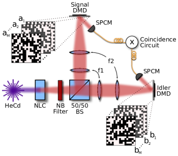
Figure 1: Experimental Setup. Photons generated via SPDC pass through a narrow-band filter and are split into signal and idler modes by a 50/50 beamsplitter. For position correlations, lenses $f1=125$ mm and $f2=500$ mm form a 4$f$ imaging system with the crystal and DMDs placed in the object and image planes respectively. For momentum correlations, f1 is removed and the DMD is placed in the focal plane of $f2=88.3$ mm. Photons striking DMD “on” pixels are directed to large area, single-photon counting modules. Photon arrivals are then correlated by a coincidence circuit.

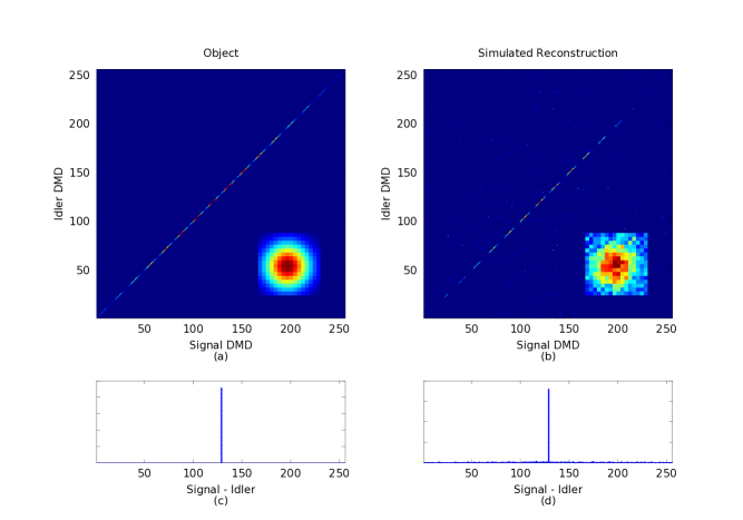
Figure 2: $16\times 16$ Pixel Simulation. The ideal object is given in (a). The object was incoherently sampled with $m=2500$ random binary patterns. Poissonian noise corresponding to 5000 photons in the field ($\approx 1250$ detected) per measurement was added to the measurement vector. The reconstruction is shown in (b), with MSE $5\times 10^{-8}$. Plots (c) and (d) integrate along the anti-diagonal to show that the reconstruction recovers the correlation width $\sigma_{c}<1$ pixel with negligible error.

;

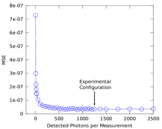
Figure 3: Simulated Mean Squared Error (MSE) versus Photon Flux for $n=256$ and $m=2500$. The phase change behavior versus photon number can be clearly seen. The experiment used $5000$ total (1250 detected) photons per measurement to comfortably exceed the phase change. The MSE approaches a value $5\times 10^{-8}$ corresponding to an SNR of roughly $17$.

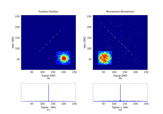
Figure 4: Sample $16\times 16$ Experimental Reconstructions. 4(a) and 4(b) give the joint probability distribution for position-position and momentum-momentum correlations where DMD pixels are listed in column-wise order. 2D marginal distributions for the signal photon are inset. 4(c) and 4(d) show correlation widths of only 1 pixel by summing over the signal $+$ idler (c) and signal $-$ idler (d) axes. Only 2500 ($3\%$ of raster-scanning) measurements were needed with a total acquisition time of about 40 minutes.

;

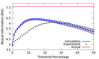
Figure 5: Mutual Information Versus Thresholding. The mutual information for reconstruction values above a thresholded percentage of the maximum is given for $100$, $n=256$ pixel simulations with $m=2500$ measurements and $\Phi=5000$ photons per measurement. The red, constant line gives the true mutual information for the simulated object. The black points give the $n=256$ far field experimental data for comparison.

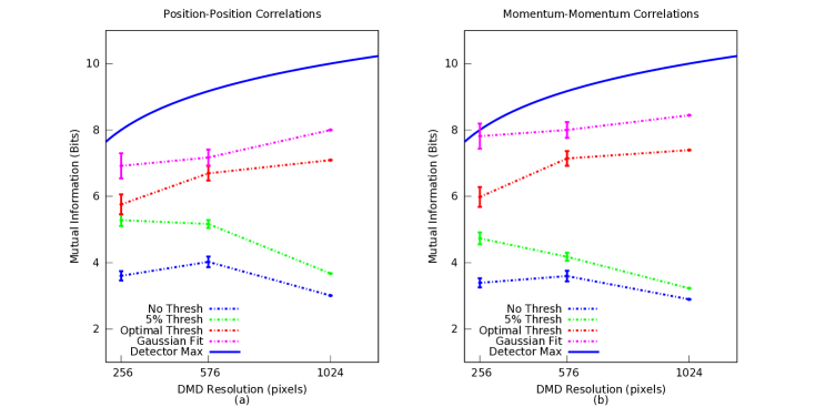
Figure 6: Mutual information between signal and idler photons for position-position and momentum-momentum representations are presented as a function of detector resolution. Three levels of thresholding are shown, as well as a fit to Eq. 5. Dashed lines are to guide the eye. Error bars enclose two standard deviations from the expected uncertainty from simulations (not performed for $n=1024$). The solid curve represents the maximum possible value for a particular detector resolution given perfect correlations and uniform marginals.

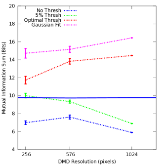
Figure 7: The sum of position-position and momentum-momentum mutual information is presented as function of detector resolution to demonstrate violation of an EPR steering inequality (Eq. 13). The solid line represents the threshold that must be exceeded to witness EPR steering. Error bars enclose two standard deviations from the expected uncertainty from simulations (not performed for $n=1024$). Because simulations systematically underestimate the mutual information, values above the bound are convincing.

The particular algorithm chosen to solve Eq. 2 also plays a role in the reconstruction”s accuracy. These often have provable performance on ideal signals, but degrade when confronted with noisy or otherwise non-ideal conditions. In these circumstances, they have various strengths, including speed, accuracy, and sensitivity to user selected parameters such as $\tau$ in Eq. 2. For more information on common reconstruction algorithms, see Refs Figueiredo et al. (2007); Candes and Wakin (2008); Li et al. (2010); Gill et al. (2011).

In practice, the best way to determine accuracy for a particular signal, sensing matrix, and reconstruction approach remains repeated simulations or experiments. For our system, we reduce a $n=32\times 32$ measurement from a $310$ day raster scan (SNR of 10) to an $8$ hour compressive acquisition, a thousand-fold improvement.

III Experiment

The experimental apparatus is given in Fig. 1. Light from a $2.8$ mW, $325$ nm HeCd laser was directed to a $1$ mm long BiBO crystal oriented for type I, collinear SPDC. The generated daughter photons passed through a $650/13$ nm narrowband filter before separating into signal and idler modes at a $50/50$ beamsplitter. To measure position-position correlations, lenses $f1=125$ mm and $f2=500$ mm imaged the crystal onto signal and idler mode DMDs. For momentum-momentum correlations, $f1$ was removed and the DMDs were placed in the focal plane of $f2=88.3$ mm. DMD “on” pixels reflected light to large area, single photon counting modules (SPCM) connected to a correlating circuit.

To measure $p(u,v)$, a series of $M$ random patterns were placed on the DMDs to form the sensing matrix $A$. For each set of patterns, joint detections were counted for acquisition times $t_{aq}$ for a total measurement time $t=Mt_{aq}$ to make up the measurement vector $y$. The joint distribution $p(u,v)$ was reconstructed using a Gradient Projection solver for Eq. 2 with $\ell_{1}$ regularization, commonly referred to as Basis Pursuit Denoising Figueiredo et al. (2007).

We measured at dimensions of $N=256^{2}$, $N=576^{2}$, and $N=1024^{2}$ corresponding to DMD resolutions of $16\times 16$, $24\times 24$, and $32\times 32$ pixels. The associated measurement numbers $M$ were $2500$, $10,000$, and $30,000$ so that $M$ is only about $0.03N$. Acquisition times were $1$ second for position measurements and $1.5$ seconds for momentum measurements to average $1000$ coincident detections per DMD configuration in all cases. Additionally, we performed representative simulations at $16\times 16$ and $24\times 24$ resolutions.

IV Results

IV.1 Joint Probability Distribution

A simulation for measuring position-position correlations at $16\times 16$ DMD resolution is given in Fig. 2. The object in 2(a) is the correlation function of Eq. 4. The simulation used $m=2500$ measurements and a photon flux of $\Phi=5000$ photons/measurement multiplied by the ideal $p(u,v)$, conditions representative of the $1$ second experimental acquisitions. Note that this is the total signal strength before interacting with the sensing matrix; the mean value of the measurement vector is $\Phi/4=1250$ detected photons. Values of the measurement vector were Poissonian distributed to simulate the effect of shot noise.

Fig. 4(b) gives the reconstructed correlation function $p(u,v$) between signal and idler DMD pixels. The sharply defined diagonal line shows the expected positive correlations between the two DMDs. DMD pixels are listed in column-major order. The mean squared error (MSE) for the reconstruction was $5\times 10^{-8}$. The two-dimensional signal marginal distribution is inset, which provides an image of the signal beam. Figs. 2(c) and 2(d) sum the result along the anti-diagonal to show the correlation width $\sigma_{c}$. Qualitatively, the reconstruction closely resembles the original object, faltering only near the edges of the distribution where the signal falls beneath a noise floor. The reconstruction recovers $\sigma_{c}<1$ pixel with negligible error.

To demonstrate the reconstruction accuracy, simulations were performed for increasing photon flux $\Phi$ with DMD resolution $16\times 16$ and $m=2500$. The MSE versus $\Phi$ is given in Fig. 3. Reconstructions were normalized to the incident flux $\Phi$ for comparison to the ideal signal. The result shows the rapid phase change from poor to excellent reconstructions with a MSE converging to $5\times 10^{-8}$ beyond the phase change.

The MSE can be used to roughly estimate the signal-to-noise ratio for a particular measurement of an average, non-zero element. Assuming perfect pixel correlations and uniform marginal distributions, the energy in the signal is distributed over $1/n$ elements. The signal-to-noise ratio is then $1/n\sqrt{\text{MSE}}$. For $n=256$ pixels and MSE $=5\times 10^{-8}$, this yields an approximate SNR of $17$. For comparison, using Eq. 9, a raster scan would require about four days to achieve a SNR of only $10$. The simulated CS acquisition time was $42$ minutes for $2500$, $1$ second measurements.

Sample experimental reconstructions for position-position and momentum-momentum correlations at $16\times 16$ pixel DMD resolution are given in Fig.4. As in the simulations, the position-position result shows a well defined diagonal line indicating positive pixel correlations. Conversely, the momentum-momentum result shows an anti-diagonal line showing the expected anti-correlations. Figs. 4(c) and 4(d) sum the results along the anti-diagonal (position-position) and diagonal (momentum-momentum) to reveal an effective correlation width $\sigma_{ce}$ of a single pixel. Our detection scheme is therefore as accurate as possible at this resolution and our channel capacity remains detector limited.

IV.2 Mutual Information in the Channel

Once $p(u,v)$ is recovered, the channel capacity is given by the classical mutual information shared between signal and idler DMD pixels;

$$I= -\sum_{u}p(u)\log p(u)-\sum_{v}p(v)\log p(v)$$

$$+\sum_{u,v}p(u,v)\log p(u,v),$$ (10)

where for example,

$$p(u)=\sum_{v}p(u,v)$$ (11)

is the signal particle’s marginal probability distribution Dixon et al. (2012). This entropic analysis is solely measurement based and does not require reconstructing a wavefunction or density matrix, a challenging task even for low-dimensional systems Barnett and Phoenix (1989); Walborn et al. (2009, 2011).

To estimate the uncertainty in the mutual information from shot noise and the reconstruction process, we performed $100$ simulations at $n=256$ pixel resolution and $31$ simulations at $n=576$ pixel resolution. Simulations were not performed at $n=1024$ pixel resolution due to available computer time. In addition to the results from the raw reconstruction, thresholding was performed to provide noise reduction, where all values in the recovered $p(u,v)$ below a percentage of the maximum value are forced to zero. The simulated mutual information versus thresholding percentage is given in Fig. 5 for the $n=256$ pixel simulations exemplified by Fig. 2. Errorbars enclose one standard deviation from repeated simulations.

As the threshold increases from zero, the mutual information rises as a weak, uncorrelated noise floor is removed. An optimal threshold is quickly reached, beyond which the threshold removes more signal than noise, reducing the mutual information. Note that the reconstructed mutual information is systematically lower than the actual mutual information in the ideal object. This is due to remaining noise and difficulty in recovering parts of the signal towards the tail of the distribution.

The $n=256$ far field experimental result is included for comparison to the simulation. The experiment closely matches the simulation both for no thresholding and beyond its optimal threshold, but is smaller in the intermediate region. This is likely due to experimental errors not included in the simulation. These include slight pixel misalignment between signal and idler DMDs, optical aberrations, detector dark noise, stray light, power fluctuations in the laser, and temperature stability of the nonlinear crystal. Fig. 5 indicates that these experimental difficulties appear to increase the uncorrelated noise floor rather than significantly affect the correlated part of the reconstruction.

Although thresholding is a simple post-processing technique, it is applicable to how the entangled pixels might be used for communication. If a pair of entangled pixels has a correlated amplitude near or below the background noise, it will be difficult to use that particular pair for communication. A communication scheme would likely only consider pixel pairs above a certain threshold to be useful. This is related to the technique in photonic quantum information of subtracting background noise from a measured signal. In CS, it is also common to perform post-processing or secondary optimization after maximizing sparsity, such as the debiasing routine used in Ref. Figueiredo et al. (2007).

The experimental channel capacity versus DMD resolution for both position-position and momentum-momentum is given in Fig. 6 for several levels of thresholding. The optimal threshold is that which maximizes the mutual information. At $256$ and $576$ pixel resolutions, optimal thresholds of $20\%$ and $30\%$ were used for position-position and momentum-momentum distributions respectively. At $1024$ pixel resolution, noise was more significant, so the optimal thresholds increased to $30\%$ and $40\%$. Error bars on $n=256$ and $n=576$ pixels measurements represent the expected effect of shot noise and reconstruction uncertainty derived from simulation. These have been conservatively set to include two standard deviations from the simulated result.

The joint probability distribution was also fit to the double-Gaussian wavefunction (Eq. 5) to find effective widths $\sigma_{ce}$ and $\sigma_{pe}$. When $\sigma_{p}\gg\sigma_{c}$, the mutual information between particles for Eq. 5 is the logarithm of the Federov ratio Fedorov et al. (2009)

$$\log\left(\frac{\sigma_{p}^{2}}{\sigma_{c}^{2}}\right),$$ (12)

where the ratio is squared for two dimensions. While this technically applies to the continuous wavefunction, and the true $\sigma_{c}$ is smaller than a DMD pixel, Eq. 12 still applies to the discritized measurement so long as the effective $\sigma_{ce}\gg\sigma_{pe}$.

Fitting yielded the largest channel capacities with a maximum of $8.4$ bits for momentum-momentum correlations at $1024$ pixel resolution, equivalent to $337$ independent, identically distributed, entangled modes.

Given that fitting more accurately characterizes the system and gives a larger mutual information, it is reasonable to question the usefulness the direct mutual information computation. However, the two approaches suit different purposes. Fitting is useful if one is particularly interested in the state itself. However, if one intends to use correlated pixels for some other purpose, such as communication, the direct calculation is more appropriate. This is because the correlated pixels on the low intensity, tail of the distribution will be difficult to use in practice even if their amplitude can be inferred by fitting.

The solid curve of Fig. 6 gives the maximum possible mutual information between two, $n$-pixel detectors. Assuming perfect diagonal or anti-diagonal correlations and uniform marginals, this is simply $\log(n)$. Because we have Gaussian marginals, we do not expect to reach this bound, even with $\sigma_{ce}\approx 1$ pixel. By magnifying and using only the central part of the field, we could approach this upper limit.

IV.3 Witnessing Entanglement

Despite not reconstructing a full density matrix, it is still possible to demonstrate non-classical behavior by comparing position-position and momentum-momentum correlation measurements directly. This has traditionally involved fitting the measurements to Eq. 5 and analyzing products or sums of conditional variances Reid (1989); Duan et al. (2000); Simon .

We recently presented a more inclusive, entropic steering inequality for witnessing continuous variable entanglement with discrete measurements Schneeloch et al. (2012), where the sum of the classical mutual information between position-position and momentum-momentum correlations is classically bounded. For our system, all classically correlated measurements must satisfy

$$I_{xs,xi}+I_{ks,ki}\leq 2\log\left(\frac{nd_{x}d_{k}}{\pi e}\right),$$ (13)

where $d_{x}$ and $d_{k}$ are the respective widths of DMD pixels in the position and momentum basis. Note that $nd_{x}d_{k}$ is simply the bandwidth product for the DMD area, and is independent of $n$ if total area does not change.

The sum of the classical mutual information in conjugate bases for each detector resolution is given in Fig. 7. The solid blue line provides right hand side of Eq. 13, which must be exceeded to witness EPR steering. Error bars for the $n=256$ and $n=576$ cases are derived from simulation and include two standard deviations. In all cases, we show EPR steering both with optimal thresholding and fitting to the double Gaussian wavefunction (Eq. 5). Even at $5\%$ thresholding, there is a violation for $16\times 16$ dimensions. Recall that simulations (Fig. 3) systematically under-represented the object mutual information relative to measurement uncertainty, so measurement error is highly unlikely to have over-estimated this sum. For the fitted $32\times 32$ dimensional result, we violate the classical bound by $6.6$ bits.

V Conclusion

In this article, we present a compressive sensing, double-pixel camera for characterizing the SPCD biphoton state with photon-counting detectors. This technique is very efficient, improving acquisition times over raster-scanning by $n^{2}/\log(n)$ for $n-$pixel detectors. We image SPDC correlations at up to 1024 dimensions per detector and measure a detector-limited mutual information of up to 8.4 bits. We also violate an entropic EPR steering bound, indicating that these correlations are non-classical. More broadly, our results suggest that compressive sensing can be extremely effective for analyzing correlations within large dimensional signals (eg. intensity-intensity correlations). Potential applications range from verifying security in spectral correlations for energy-time QKD Ali-Khan et al. (2007) to imaging through scattering media Gong and Han (2011).

This work was supported by DARPA InPho grant W911NF-10-1-0404.

References

- Einstein et al. (1935) A. Einstein, B. Podolsky, and N. Rosen, “Can Quantum-Mechanical Description of Physical Reality Be Considered Complete?” Phys. Rev. 47, 777–780 (1935).
- Howell et al. (2004) J. C. Howell, R. S. Bennink, S. J. Bentley, and R. W. Boyd, “Realization of the Einstein-Podolsky-Rosen Paradox Using Momentum- and Position-Entangled Photons from Spontaneous Parametric Down Conversion,” Phys. Rev. Lett. 92, 210403 (2004).
- Pors (2011) J. B. Pors, Entangling Light in High Dimensions, Ph.D. thesis, Leiden University (2011).
- Ekert (1991) A. K. Ekert, “Quantum Cryptography Based on Bell’s Theorem,” Phys. Rev. Lett. 67, 661–663 (1991).
- Walborn et al. (2006) S. P. Walborn, D. S. Lemelle, M. P. Almeida, and P. H. Souto Ribeiro, “Quantum Key Distribution with Higher-Order Alphabets Using Spatially Encoded Qudits,” Phys. Rev. Lett. 96, 090501 (2006).
- Walborn et al. (2008) S. P. Walborn, D. S. Lemelle, D. S. Tasca, and P. H. Souto Ribeiro, “Schemes for Quantum Key Distribution with Higher-order Alphabets Using Single-photon Fractional Fourier Optics,” Phys. Rev. A 77, 062323 (2008).
- Bennett and Wiesner (1992) C. H. Bennett and S. J. Wiesner, “Communication via One- and Two-particle Operators on Einstein-Podolsky-Rosen States,” Phys. Rev. Lett. 69, 2881–2884 (1992).
- Braunstein and Kimble (2000) S. L. Braunstein and H. J. Kimble, “Dense Coding for Continuous Variables,” Phys. Rev. A 61, 042302 (2000).
- Pittman et al. (1995) T. B. Pittman, Y. H. Shih, D. V. Strekalov, and A. V. Sergienko, “Optical Imaging by Means of Two-photon Quantum Entanglement,” Phys. Rev. A 52, R3429–R3432 (1995).
- Abouraddy et al. (2001) A. F. Abouraddy, B. E. A. Saleh, A. V. Sergienko, and M. C. Teich, “Role of Entanglement in Two-Photon Imaging,” Phys. Rev. Lett. 87, 123602 (2001).
- Tasca et al. (2011) D. S. Tasca, R. M. Gomes, F. Toscano, P. H. Souto Ribeiro, and S. P. Walborn, “Continuous-variable Quantum Computation with Spatial Degrees of Freedom of Photons,” Phys. Rev. A 83, 052325 (2011).
- Walborn et al. (2007) S. P. Walborn, D. S. Ether, R. L. de Matos Filho, and N. Zagury, “Quantum Teleportation of the Angular Spectrum of a Single-photon Field,” Phys. Rev. A 76, 033801 (2007).
- Di Lorenzo Pires et al. (2009) H. Di Lorenzo Pires, C. H. Monken, and M. P. van Exter, “Direct Measurement of Transverse-mode Entanglement in Two-photon States,” Phys. Rev. A 80, 022307 (2009).
- Coffey (2011) V. C. Coffey, “Seeing in the Dark: Defense Applications of IR Imaging,” Opt. Photonics News 22, 26–31 (2011).
- Albota (2002) M. A Albota, “Three-Dimensional Imaging Laser Radars with Geiger-Mode Avalange Photodiode Arrays,” Lincoln Laboratory Journal 13, 351 –367 (2002).
- Itzler et al. (2010) M. A. Itzler, M. Entwistle, M. Owens, K. Patel, X. Jiang, K. Slomkowski, S. Rangwala, P. F. Zalud, T. Senko, J. Tower, and J. Ferraro, “Geiger-mode Avalanche Photodiode Focal Plane Arrays for Three-dimensional Imaging LADAR,” in Proc. SPIE, Infrared Remote Sensing and Instrumentation XVIII, Vol. 7808 (SPIE, 2010) p. 78080C.
- Edgar et al. (2012) M. P. Edgar, D. S. Tasca, F. Izdebski, R. E. Warburton, J. Leach, M. Agnew, G. S. Buller, R. W. Boyd, and M. J. Padgett, “Imaging High-dimensional Spatial Entanglement with a Camera,” Nat. Commun. 3 (2012), 10.1038/ncomms1988.
- Dixon et al. (2012) P. B. Dixon, G A. Howland, J. Schneeloch, and J. C. Howell, “Quantum Mutual Information Capacity for High-Dimensional Entangled States,” Phys. Rev. Lett. 108, 143603 (2012).
- Bellman (2003) R. Bellman, Dynamic Programming (Dover Books on Computer Science) (Dover Publications, 2003).
- Schneeloch et al. (2012) J. Schneeloch, P. B. Dixon, G. A. Howland, C. J. Broadbent, and J. C. Howell, “Witnessing Continuous Variable Entanglement with Discrete Measurements,” (2012), arXiv, arXiv:quant-ph/1210.4234 .
- Donoho (2006) D. L. Donoho, “Compressed Sensing,” Information Theory, IEEE Transactions on 52, 1289 –1306 (2006).
- Candes and Romberg (2007) E. J. Candes and J. Romberg, “Sparsity and Incoherence in Compressive Sampling,” Inverse Problems 23, 969 (2007).
- Baraniuk (2007) R.G. Baraniuk, “Compressive Sensing [Lecture Notes],” Signal Processing Magazine, IEEE 24, 118 –121 (2007).
- Candes and Wakin (2008) E. J. Candes and M. B. Wakin, “An Introduction To Compressive Sampling,” Signal Processing Magazine, IEEE 25, 21 –30 (2008).
- Candes and Romberg (2005) E. J. Candes and J. Romberg, “l1-Magic: Recovery of Sparse Signals via Convex Programming,” (2005).
- Candes et al. (2006) E.J. Candes, J. Romberg, and T. Tao, “Robust Uncertainty Principles: Exact Signal Reconstruction from Highly Incomplete Frequency Information,” Information Theory, IEEE Transactions on 52, 489 – 509 (2006).
- Gross et al. (2010) D. Gross, Y. K. Liu, S. T. Flammia, S. Becker, and J. Eisert, “Quantum State Tomography via Compressed Sensing,” Phys. Rev. Lett. 105, 150401 (2010).
- Shabani et al. (2011) A. Shabani, R. L. Kosut, M. Mohseni, H. Rabitz, M. A. Broome, M. P. Almeida, A. Fedrizzi, and A. G. White, “Efficient Measurement of Quantum Dynamics via Compressive Sensing,” Phys. Rev. Lett. 106, 100401 (2011).
- Katz et al. (2009) O. Katz, Y. Bromberg, and Y. Silberberg, “Compressive Ghost Imaging,” Applied Physics Letters 95, 131110 (2009).
- Zerom et al. (2011) P. Zerom, K. W. C. Chan, J. C. Howell, and R. W. Boyd, “Entangled-photon Compressive Ghost Imaging,” Phys. Rev. A 84, 061804 (2011).
- Wakin et al. (2006) M.B. Wakin, J.N. Laska, M.F. Duarte, D. Baron, S. Sarvotham, D. Takhar, K.F. Kelly, and R.G. Baraniuk, “An Architecture for Compressive Imaging,” in Image Processing, 2006 IEEE International Conference on (2006) pp. 1273 –1276.
- Duarte et al. (2008) M. F. Duarte, M. A. Davenport, D. Takhar, J. N. Laska, T. Sun, K. F. Kelly, and R. G. Baraniuk, “Single-Pixel Imaging via Compressive Sampling,” Signal Processing Magazine, IEEE 25, 83 –91 (2008).
- Duarte and Baraniuk (2010) M.F. Duarte and R.G. Baraniuk, “Kronecker product matrices for compressive sensing,” in Acoustics Speech and Signal Processing (ICASSP), 2010 IEEE International Conference on (2010) pp. 3650 –3653.
- Duarte and Baraniuk (2012) M.F. Duarte and R.G. Baraniuk, “Kronecker compressive sensing,” Image Processing, IEEE Transactions on 21, 494 –504 (2012).
- Li et al. (2010) C. Li, W. Yin, and Y. Zhang, “TVAL3: TV Minimization by Augmented Lagrangian and ALternating Direction ALgorithms,” (2010).
- Horn and Johnson (1994) R. A. Horn and C. R. Johnson, Topics in Matrix Analysis (Cambridge University Press, 1994).
- Willett et al. (2011) Rebecca M. Willett, Roummel F. Marcia, and Jonathan M. Nichols, “Compressed sensing for practical optical imaging systems: a tutorial,” Optical Engineering 50, 072601–072601–13 (2011).
- Donoho et al. (2011) D.L. Donoho, A. Maleki, and A. Montanari, “The noise-sensitivity phase transition in compressed sensing,” Information Theory, IEEE Transactions on 57, 6920 –6941 (2011).
- Wu and Verdu (2012) Yihong Wu and S. Verdu, “Optimal phase transitions in compressed sensing,” Information Theory, IEEE Transactions on 58, 6241 –6263 (2012).
- Reeves and Gastpar (2012) G. Reeves and M. Gastpar, “Compressed sensing phase transitions: Rigorous bounds versus replica predictions,” in Information Sciences and Systems (CISS), 2012 46th Annual Conference on (2012) pp. 1 –6.
- Willett and Raginsky (2009) R.M. Willett and M. Raginsky, “Performance bounds on compressed sensing with poisson noise,” in Information Theory, 2009. ISIT 2009. IEEE International Symposium on (2009) pp. 174 –178.
- Harmany et al. (2009) Z.T. Harmany, R.F. Marcia, and R.M. Willett, “Sparse poisson intensity reconstruction algorithms,” in Statistical Signal Processing, 2009. SSP ’09. IEEE/SP 15th Workshop on (2009) pp. 634 –637.
- Ganguli and Sompolinsky (2010) Surya Ganguli and Haim Sompolinsky, “Statistical mechanics of compressed sensing,” Phys. Rev. Lett. 104, 188701 (2010).
- Figueiredo et al. (2007) M. A. T. Figueiredo, R. D. Nowak, and S. J. Wright, “Gradient Projection for Sparse Reconstruction: Application to Compressed Sensing and Other Inverse Problems,” Selected Topics in Signal Processing, IEEE Journal of 1, 586–597 (2007).
- Gill et al. (2011) P.R. Gill, A. Wang, and A. Molnar, “The in-crowd algorithm for fast basis pursuit denoising,” Signal Processing, IEEE Transactions on 59, 4595 –4605 (2011).
- Barnett and Phoenix (1989) S. M. Barnett and S. J. D. Phoenix, “Entropy as a Measure of Quantum Optical Correlation,” Phys. Rev. A 40, 2404–2409 (1989).
- Walborn et al. (2009) S. P. Walborn, B. G. Taketani, A. Salles, F. Toscano, and R. L. de Matos Filho, “Entropic Entanglement Criteria for Continuous Variables,” Phys. Rev. Lett. 103, 160505 (2009).
- Walborn et al. (2011) S. P. Walborn, A. Salles, R. M. Gomes, F. Toscano, and P. H. Souto Ribeiro, “Revealing Hidden Einstein-Podolsky-Rosen Nonlocality,” Phys. Rev. Lett. 106, 130402 (2011).
- Fedorov et al. (2009) M. V. Fedorov, Yu. M. Mikhailova, and P. A. Volkov, “Gaussian Modelling and Schmidt Modes of SPDC Biphoton States,” Journal of Physics B: Atomic, Molecular and Optical Physics 42, 175503 (2009).
- Reid (1989) M. D. Reid, “Demonstration of the Einstein-Podolsky-Rosen Paradox Using Nondegenerate Parametric Amplification,” Phys. Rev. A 40, 913–923 (1989).
- Duan et al. (2000) Lu-Ming Duan, G. Giedke, J. I. Cirac, and P. Zoller, “Inseparability criterion for continuous variable systems,” Phys. Rev. Lett. 84, 2722–2725 (2000).
- (52) R. Simon, “Peres-horodecki separability criterion for continuous variable systems,” Phys. Rev. Lett. 84.
- Ali-Khan et al. (2007) I. Ali-Khan, C. J. Broadbent, and J. C. Howell, “Large-Alphabet Quantum Key Distribution Using Energy-Time Entangled Bipartite States,” Phys. Rev. Lett. 98, 060503 (2007).
- Gong and Han (2011) W. Gong and S. Han, “Correlated Imaging in Scattering Media,” Opt. Lett. 36, 394–396 (2011).