Multi-thermal dynamics and energetics
of a coronal mass ejection in the low solar atmosphere

Abstract

Aims. The aim of this work is to determine the multi-thermal characteristics and plasma energetics of an eruptive plasmoid and occulted flare observed by Solar Dynamics Observatory/Atmospheric Imaging Assembly (SDO/AIA).

Methods. We study an event from 03-Nov-2010 (peaking at 12:20UT in GOES soft X-rays) of a coronal mass ejection and occulted flare which demonstrates the morphology of a classic erupting flux rope. The high spatial, and time resolution, and six coronal channels, of the SDO/AIA images allows the dynamics of the multi-thermal emission during the initial phases of eruption to be studied in detail. The Differential Emission Measure (DEM) is calculated, using an optimised version of a regularized inversion method (Hannah & Kontar 2012), for each pixel across the six channels at different times, resulting in emission measure maps and movies in a variety of temperature ranges.

Results. We find that the core of the erupting plasmoid is hot (8-11, 11-14MK) with a similarly hot filamentary “stem” structure connecting it to the lower atmosphere, which could be interpreted as the current sheet in the flux rope model, though is wider than these models suggest. The velocity of the leading edge of the eruption is 597-664 km s^-1 in the temperature range $\geq$3-4MK and between 1029-1246 km s^-1 for $\leq$2-3MK. We estimate the density (in 11-14 MK) of the erupting core and stem during the impulsive phase to be about $3\times 10^{9}$ cm^-3, $6\times 10^{9}$ cm^-3, $9\times 10^{8}$ cm^-3 in the plasmoid core, stem and surrounding envelope of material. This gives thermal energy estimates of $5\times 10^{29}$ erg, $1\times 10^{29}$ erg and $2\times 10^{30}$ erg. The kinetic energy for the core and envelope is slightly smaller. The thermal energy of the core and current sheet grows during the eruption, suggesting continuous influx of energy presumably via reconnection.

Conclusions. The combination of the optimised regularized inversion method and SDO/AIA data allows the multi-thermal characteristics (i.e. velocity, density and thermal energies) of the CME eruption to be determined.

1 Introduction

The solar atmosphere is awash with highly dynamic phenomena driven by the rapid liberation of magnetically stored energy. Magnetic reconnection is thought to facilitate this energy release, resulting in solar flares, coronal mass ejections (CMEs) and the associated particle acceleration, plasma heating and bulk motions. The classic model of solar eruptive events (SEE) is the CSHKP model (Carmichael 1964; Sturrock 1966; Hirayama 1974; Kopp & Pneuman 1976) which continues to become more ornate over time (for instance Lin & Forbes 2000). The basic scenario is that of an erupting flux rope (helical magnetic structure) which stretches and elongates the coronal magnetic field behind it, instigating magnetic reconnection in a vertical current sheet. This releases considerable energy, particularly in accelerated particles that then travel down into the denser lower solar atmosphere. Here they lose their energy through collisions with the background plasma, producing hard X-ray (HXR) footpoints and flare ribbons, heating material that then expands upwards filling flaring loops.

Flares are well observed in the lower solar atmosphere, but CMEs have, till recently, mostly been studied at higher altitudes (for an overview see Hudson et al. (2006); Webb & Howard (2012)) due to the lack of suitable high cadence observations. This means that there is considerable uncertainty as to the specific processes that develop flux ropes and initiate CMEs (e.g Démoulin & Aulanier 2010). High in the corona, white-light observations typically show CMEs structured as a bright loop ahead of a darker cavity containing a bright core. Here the bright loop is taken to be due to the increased density of material amassed in the leading front of the eruption with the cavity likely due to to a flux rope (Gibson et al. 2006). CMEs have been found to evolve in distinct stages, initiation, acceleration and propagation (Zhang & Dere 2006) and the initial acceleration stage of CME synchronize well with the flare HXR (Kahler et al. 1988; Sterling & Moore 2005; Temmer et al. 2008, 2010) and soft X-ray (SXR) emission (Zhang et al. 2001; Vršnak et al. 2005), while the HXR flux correlates with the acceleration of CMEs (Temmer et al. 2010). Active regions are significantly more likely to be eruptive if they have a sigmoidal morphologly (Canfield et al. 1999) and these structures are seen as the precursors to flux ropes both observational (Liu et al. 2010; Green et al. 2011) and in simulations (Török & Kliem 2003; Fan & Gibson 2003; Archontis & Török 2008; Aulanier et al. 2010).

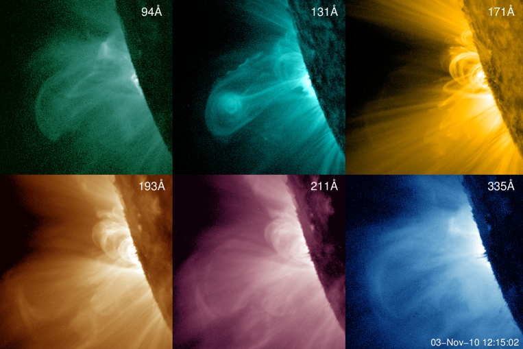
Figure 1: SDO/AIA observations from each of the six coronal filters during the impulsive phase of the 3-Nov-2010 flare when the erupting plasmoid is clearly visible in 131Å. The time shown is for the 94Å  image, with all from 12:15:00 to 12:15:09UT.

Associated with CMEs is the nearby dimming of the corona during the onset stage, seen in soft X-rays (Sterling & Hudson 1997) and EUV (e.g. Gopalswamy & Hanaoka 1998). This could be due to the depletion of material as part of the eruption, plasma heating or a combination of both. Observations generally point to the former: for instance five CMEs studied by Harrison et al. (2003) using EUV spectroscopic data from CDS showed dimming due to mass loss and not temperature variations. However the are also examples of CMEs where the dimming is due to plasma heating and not depletion (Robbrecht & Wang 2010).

Spectral observations of CMEs in the extended corona ($>1.5R_{\sun}$ from Sun centre) with SOHO/UVCS revealed many aspects of CMEs at these altitudes (Kohl et al. 2006), observing spectral lines from CMEs over 0.02 – 6 MK. In one CME a “narrow” (100Mm) structure was observed for 20hrs, with an emission measure of about $10^{25}$cm^-5 over 4 – 6 MK connecting the CME core to the flare loops below (Ciaravella et al. 2002). This was interpreted as an edge-on view of the current sheet and a density of $5\times 10^{7}$cm^-3 was estimated using a 40Mm line-of-sight component. Similarly hot current sheets have been observed in another long-duration event (Ko et al. 2003) as well as faster ones (Lin et al. 2005) where the leading edge and CME core were moving at 1 939 and 1 484 kms^-1 respectively. Hotter current sheets have been observed in some CMEs as well (Innes et al. 2003; Bemporad et al. 2006; Schettino et al. 2010). Landi et al. (2010) used Hinode/EIS to determine the Differential Emission Measure (DEM, see §2) of the CME lower in the solar atmosphere (at $1.1R_{\sun}$). They found a multiple peaked DEM, with two components at 0.13 MK of density $10^{10-11}$ cm^-3 and another at 0.5 MK of density $10^{8.7}$ cm^-3 travelling together. The emission at about 1MK was due to the line-of-sight/background corona however SXR emission was also detected by Hinode/XRT, enveloping the core and suggestive of material at 5–10 MK. The analysis of the post eruption arcade found similar plasma to the current sheet, both coronal plasma heated up to 3 MK (Landi et al. 2012)

High spatial ($\sim 1.5\arcsec$) and temporal resolution ($\sim 12$ s) EUV full disk images in multiple wavelengths is now available from the Atmospheric Imaging Assembly (Lemen et al. 2012) on the Solar Dynamics Observatory (SDO/AIA), with several authors taking advantage of this data to study CME formation and propagation from the low corona (e.g. Patsourakos et al. 2010; Kozarev et al. 2011). One particular event, which peaked in GOES SXRs at 12:20UT 03-Nov-2010 (Figure 1), of an occulted flare and erupting plasmoid, shows unambiguously the formation of a flux rope and has subsequently been studied in detail (Reeves & Golub 2011; Cheng et al. 2011; Foullon et al. 2011; Bain et al. 2012; Savage et al. 2012; Cheng et al. 2012), and will be studied in detail in this paper. This event shows the formation of a flux rope clearly in 131Å, images with a peak in their sensitivity at 11MK, though dimming at the core in channels sensitive to cooler emission (171Å, 211Å), shown in Figure 1. As the plasmoid move outwards, a filamentary, stem-like structure forms behind it, again sharply defined in 131Å, suggestive of a large-scale current sheet (Reeves & Golub 2011; Cheng et al. 2011; Savage et al. 2012). The kinematics of the eruption in the different channels has been found to be slower (about 600 kms^-1 versus 1 400 kms^-1) in those sensitive to hotter emission (Cheng et al. 2011; Bain et al. 2012).

The propagation of a metric Type II radio burst ahead of the CME in EUV is faster still (nearing 2 000 kms^-1) suggesting a piston-drive shock, in which it is moving too quickly for the ambient plasma to flow behind the driver (Bain et al. 2012). This work also found that HXR emission observed with RHESSI had two non-thermal (18-40 keV) sources, one compact low in the corona, the other extended and high in the corona, close to the erupting plasmoid. The later could be due to electrons accelerated in the stem/current sheet. Although this event superficially matches the cartoon model of flux rope eruption things are more complicated: Foullon et al. (2011) found Kelvin-Helmholtz waves along the top edge of the erupting plasma, possibly allowing a secondary reconnection process. Savage et al. (2012) studied the inflow and outflow into the CS region, finding the hottest material inflowing fastest and correlating with the RHESSI thermal X-ray emission. Pairs of inflowing and outflowing material was found to be travelling away from the region faster than they arrived, suggesting acceleration.

Since SDO/AIA provides six different wavelength channels, sensitive to a range of coronal temperatures, they can be used to determine the DEM of the different parts of the CME. Cheng et al. (2012) did this for this event, as well as two others, producing DEMs for different CME regions: the core of the erupting flux rope and the leading front. They found the cores to be have emission over a broad distribution of temperatures ($3\leq T\leq 20$MK), with an average temperature of about $>8$MK and densities of about $10^{9}$cm^-3. The leading front of the eruptions were cooler (about 2MK on average) with a narrower temperature distribution ($1\leq T\leq 3$MK) similar to the pre-eruption coronal material but with slightly higher densities. They interpreted the leading fronts to be the showing signatures of compressed ambient coronal plasma. Dimming, about 10 minutes after the eruption, was found to be due to the rarefaction of material.

In this paper we use a different approach, regularized inversion, to produce the DEM not for a few regions within the CME but for every single pixel in the set of six SDO/AIA images, every 12 seconds throughout the event. Thus allowing the highly dynamic multi-thermal properties of the CME to be investigated. The regularized approach detailed in this paper (see§2) is an optimized version of our original code, introduced, tested, and compared to the approach used by Cheng et al. (2012) in Hannah & Kontar (2012). The version present here is able to compute 10 000s of DEMs per second, calculating both horizontal and vertical and uncertainties (see §2.2) and without forcing a prescribed DEM model. In §3.2 the properties of the DEM in different pixels of the event are discussed, with the maps and their uncertainties presented in §3.3. We then investigate the time evolution of the DEMs in terms of the morphology, total emission and propagation speed for the different temperature ranges, in §3.4. As the erupting plasmoid and filamentary stem structure is well defined at high temperature (11-14MK), we use the emission measures in §3.5 to estimate the densities and thermal energy of the different components.

2 Differential Emission Measures

2.1 Introduction

The signal detected $g(x,y,t,i)$ in each pixel $(x,y)$ in the $i^{th}$ SDO/AIA filter at time $t$ can be interpreted as

$$g(x,y,t,i)=\int_{T}K(T,i)\xi(T,x,y,t)dT+\delta g(x,y,t,i),$$ (1)

where $K(T,i)$ is the temperature response of the $i^{th}$ filter (O’Dwyer et al. 2010; Boerner et al. 2012). The Differential Emission Measure DEM $\xi(T,x,y,t)$, at a particular instance in one pixel, is taken to be $\xi(T)=n(h)^{2}\mathrm{d}h/\mathrm{d}T$ [cm^-5K^-1], which is the electron density $n^{2}$ along the line-of-sight $h$ of the emitting material at temperature $T$. The inherent noise in the observations $\delta g(x,y,t,i)$, due to counting statistics, background and instrumental uncertainties, will be significantly amplified when a direct solution of Eq. (1) is attempted. This recovery of the DEM is an ill-posed inverse problem (Tikhonov 1963; Bertero et al. 1985; Craig & Brown 1986; Prato et al. 2006) with the growth of uncertainties resulting in spurious solutions. To recover useful solutions of the problem given in Eq. (1), it needs to be constrained to avoid the noise amplification in the DEM solution. The constraints are often physically motivated additional information a priori known about the solution. An additional challenge here is that we need an approach that can quickly and robustly calculate DEMs since there is a wealth of SDO/AIA data to study this highly dynamic eruption. The simple isothermal/ratio approach (e.g. Vaiana et al. 1973) places a very strict, though possibly erroneous, constraint on the DEM solution and so is ill-suited to this problem. An alternative is to forward fit a chosen DEM model to the data, for example with multi-Gaussians (e.g. Aschwanden & Boerner 2011) or splines (e.g. Weber et al. 2004), the latter used for this CME event by Cheng et al. (2012). Again, if the assumption about the form of the DEM is wrong then the results are difficult to reliably interpret. These techniques can be computationally slow, only allowing select regions to be analysed, not taking full advantage of the SDO/AIA data. Other approaches, such as MCMC (Kashyap & Drake 1998), can produce very robust results, without requiring predefined functional forms to the DEM solution, and uncertainty estimates but are computationally slow and so are again inappropriate to obtain DEM maps.

Tikhonov regularized inversion recovers the solution by limiting the amplification of the uncertainties through assumptions about its “smoothness” by using linear constraints (Tikhonov 1963; Craig 1977; Prato et al. 2006). This approach does not make any assumption on the functional form of DEM and we have implemented an algorithm (Hannah & Kontar 2012) to recover the DEM from solar data using Tikhonov regularization and Generalized Singular Value Decomposition GSVD (Hansen 1992). This code, originally developed and extensively tested for the inversion of X-ray data (Kontar et al. 2004, 2005), naturally provides estimates to the uncertainties in the solution, an important feature, when trying to recover a large number of DEMs. Recently, a simpler and computationally fast (computing 100s to 1,000s DEMs per second) SVD regularisation approach has been applied to AIA data (Plowman et al. 2012), however it does not produce error estimates. Regularization has also been used with solar data to determine the 3D emission measure through the use of solar rotation or multi-spacecraft observations (Frazin et al. 2005, 2009). In general, regularized approaches do not require a positive solution but one can be obtained by using an iterative method such a Reiterated Conjugate Gradients, which was used for solar data by Fludra & Sylwester (1986). Our approach uses one iteration to help with the weighting, and positivity, of the final solution whilst maintaining the fast computational speed.

2.2 Regularization Method for DEM maps

The full details of the method are in Hannah & Kontar (2012) and this previous version of the algorithm allows a variety of different controls to the nature of the regularization but is too computationally slow to practically produce DEM maps and movies (running at about a few DEMs per second). We have produced an optimized and simplified version of the software, detailed below with considerable speed gains. As the DEM calculation per pixel location is independent of other pixels in the same image, further speed gains were achieved by parallization of the code within IDL using Bridges. The results is that we can achieve about 1 000s DEMs per second on a standard multi-core cpu laptop/desktop and 10 000s on multi-cpu machines.

To obtain the DEM maps we perform regularization with the zeroth-order constraint and no initial guess solution. For the detailed explanation of these parameters and the affect they have on the regularized solution see Hannah & Kontar (2012). The specific problem to be solved here is

$$\left\|{\bf\widetilde{K}}\;{\xi-\bf\widetilde{g}}\right\|^{2}+\lambda\|{{{\bf L}\;\xi}}\|^{2}=\mbox{min},$$ (2)

where the constraint matrix ${\bf L}$ is the identity matrix (normalised by the temperature bin width) and the tilde indicates normalisation by the error in the data $\delta g$. The GSVD singular values ($\gamma_{i}$, $\beta_{i}$) and vectors ($\bf u,v,w$) produced from the GSVD of $\bf\widetilde{K}$ and $\bf L$ provide a ready DEM solution $\xi_{\lambda}$ as a function of the regularisation parameter $\lambda$ (Hansen 1992), i.e.

$$\xi_{\lambda}(T)=\sum_{i=1}^{6}\frac{\phi_{i}^{2}}{\phi_{i}^{2}+\lambda}\left(\frac{({\bf\widetilde{g}}\cdot{\bf u}_{i}){\bf w}_{i}}{\gamma_{i}}\right)\;,$$ (3)

where $\phi_{i}=\gamma_{i}/\beta_{i}$. To find the regularization parameter $\lambda$ that produces a solution $\xi_{\lambda}$ that matches the required $\chi^{2}=1$ (in data space) we use coarser sampling of $\lambda$ than in the original software which helps with the computational speed increase. Even with this approach we achieve $\chi^{2}$ of typically between 0.5 and 1.75 with our regularized solutions, which are identical (within the error bars) to the results from the previous code. The above procedure is run twice (as in the original code) with the result from the first run $\xi_{\lambda}(T)$ being used to weight the constraint matrix as $\mathbf{L}^{2}_{jj}=d\log{T_{j}}/\xi_{\lambda}(T_{j})$ before the second GSVD is performed and final $\xi_{\lambda}$ solution found. The horizontal errors are again taken to be the spread of the resolution matrix $\mathbf{R_{\lambda}K}$ for each temperature bin (Hannah & Kontar 2012), where $\mathbf{R_{\lambda}}$ is the regularized inverse assumed to be close to the generalized inverse $\mathbf{K^{\dagger}}$, i.e. $\xi_{\lambda}\simeq\mathbf{R_{\lambda}g}$. For the vertical error we do not use the Monte Carlo approach as in Hannah & Kontar (2012) but take it to be $\Delta\xi(T)^{2}=<\delta\xi(T)^{2}>=\left\|\mathbf{R_{\lambda}\delta g}\right\|^{2}$. This produces a similar result but is considerably quicker to compute.

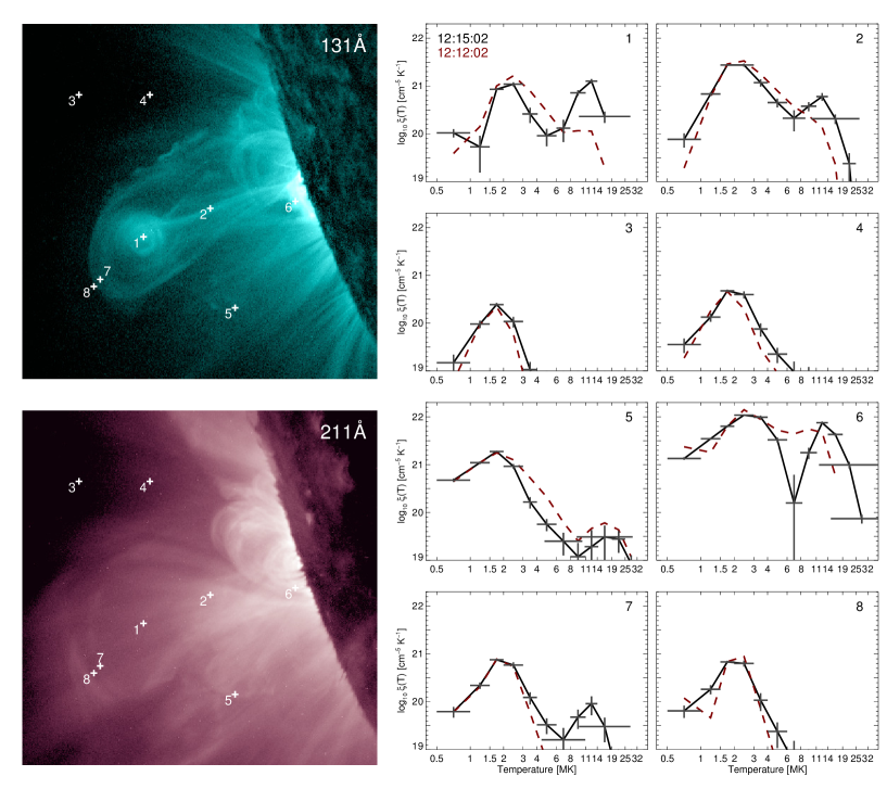
Figure 2: (Left) The 131Å and 211Å images from Figure 1 with eight pixels highlighted. (Right) The corresponding regularized DEM solutions $\xi(T)$ (using twelve temperature bins) and the vertical $\Delta\xi(T)$ and horizontal $\Delta\log{T}$ errors (the maximum of the error from the resolution matrix or the temperature bin width) for the highlighted pixels using the data from all six image in Figure 1. The dashed lines show the DEM solutions in those pixels before the eruption at 12:12:02 UT whereas the solid lines are from 12:15:02 UT.

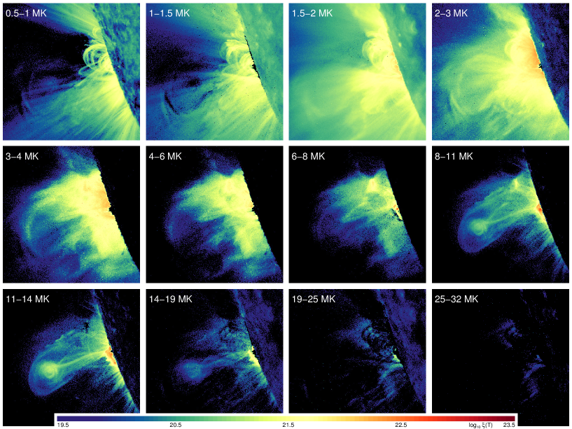
Figure 3: DEM maps in different temperature ranges for the 3-Nov-2010 flare at 12:15:02 UT. The same pixel position in the twelve maps corresponds to the regularized DEM solution $\xi(T)$ (as shown in detail for eight pixel positions in Figure 2) to the set of data values from the corresponding pixel in the six images shown in Figure 1. The colour scale is $\log{\xi(T)}$ and is in units of cm^-5K^-1.

3 DEM Maps of 03-Nov-2010 Eruptive Event

3.1 Data Reduction

The data between 12:12:02 UT and 12:19:02 UT (with a set of six different channel images every 12 seconds) were prepared to level 1.6 by deconvolving the point spread function using aia_deconvolve_richardsonlucy.pro before being processed with aia_prep.pro. The co-alignment of the images were checked using aia_coalign_test.pro and found to be sub-pixel accurate. The resulting images were reduced down to sub-maps covering -1150″to -850″in the x direction and and -500″to -200″in the y direction, 501 by 501 pixels.

For each pixel position $(x,y)$ across the six different filters ($i=1\ldots 6$) in the 12 second set $t$ provides the signal $g(x,y,t,i)$, in units of DN s^-1px^-1, from which the associated errors $\delta g(x,y,t,i)$ are calculated using the readout noise and photon counting statistics. The set of six values, and their associated errors, with the temperature response functions are passed to the regularized DEM map code, as detailed in §2. The SDO/AIA temperature response functions are calculated using both the CHIANTI fix (an empirical correction for missing emission in the CHIANTI v7.0 database in channels 94Å  and 131Å) and EVE normalisation (to match EVE spectroscopic full-disk observations), further details available online.. We use fairly broad temperature binning, twelve pseudo-logarithmic bins between 0.5 to 32MK, as to avoid a large number of temperature bins slowing down the code. These are larger than the designed achievable temperature resolution (Judge 2010), yet narrow enough to recover test models , from testing the recovery of Gaussian model DEMs, as in Hannah & Kontar (2012).

3.2 DEM from individual pixels

The resulting DEMs found for eight distinct pixel locations in the images from Figure 1 are shown in Figure 2. These pixels are shown for the 131Å and 211Å images but the data from all six coronal-filter images were used to recover the DEMs. The vertical and horizontal errors shown are calculated as detailed in §2.2. The vertical error is just the linear propagation of the uncertainty on the source data but the horizontal error is more complicated as it gives a measure of the temperature spread (from the resolution matrix) as well as the quality of the regularized solution (i.e. strong off-diagonal terms) in each bin, see Hannah & Kontar (2012) for further details. The DEMs of the different positions show a variety of forms but clearly none are isothermal and the majority cannot be represented by a single Gaussian model. Shown for comparison are the DEMs obtained in these pixels before the eruption at 12:12:02 UT.

For each specific pixel we have:

Pixel 1 - Core of the erupting plasmoid:

There are clearly two distinct components, one peaking in the range 1.5-3MK, the other at 8-14MK. The lower temperature one is likely the background corona along the line-of-sight whereas the hotter from the plasmoid itself. The pre-eruption DEM has no high temperature component;

Pixel 2 - Filament/stem behind the plasmoid:

Again two components at similar temperature ranges to the core of the plasmoid but the low temperature component has larger emission (due to higher densities lower in the corona compared to Pixel 1) and the higher temperature one has considerably weaker emission (due to a smaller amount of heated material accumulating in this location compared to the core, Pixel 1). The pre-eruption DEM has no high temperature component;

Pixel 3 - High corona away from the event:

A single component covering 1-3MK with expected weak emission, since lower density higher in the corona, and identical (within the errors bars) to the pre-eruption DEM;

Pixel 4 - Corona away from the event:

A broader DEM with slightly higher peak emission than Pixel 3, likely due to it being lower in the corona but again peaking over 1-3MK, and similar (within the errors bars) to the pre-eruption DEM;

Pixel 5 - Corona near the event:

Higher emission and broader DEM than similar location of Pixel 4 indicating the presence of more hot coronal loops. The emission at high temperatures (above 6MK) is zero within the errors bars. The pre-eruption DEM is slightly higher, though consistent within the errors, so may indicate a slightly hotter and denser loop(s) moving out of this region;

Pixel 6 - Low corona flare emission:

Very high emission across all temperatures with a bright peak at 1.5-3MK and 8-14MK for the flare heated material expanding up above the limb to be visible. The pre-eruption DEM shows emission across 6-8MK and 8-11MK but weaker at higher temperatures, which might be due to the behind-the-limb flare;

Pixel 7 - Envelope just ahead of the plasmoid:

Weaker emission than the core of the plasmoid (Pixel 1) but again a similar DEM with two components, peaking at 1.5-3MK and 8-14MK, the latter likely due to the accumulation of hotter coronal emission in this leading front of the eruption. The pre-eruption DEM does not show this hotter (8-14MK) emission;

Pixel 8 - Further ahead of the plasmoid:

Similar to the low temperature component of Pixel 7 (which is physically closer to the core of the erupting material) but no higher temperature component. Consistent (within the error bars) to the pre-eruption DEM.

Overall the DEMs in Figure 2 present a similar scenario to that found by previous authors (Cheng et al. 2011; Bain et al. 2012) who were studying the behaviour just in the different SDO/AIA channels, as well as the DEM analysis from Cheng et al. (2012). Given the inherent difficulties in recovering DEMs this is reassuring that their bulk features are consistent with the original SDO/AIA data. Here we have a hot (8-11, 11-14MK) plasmoid core, well-defined with a filamentary stem-like structure behind it, similarly hot. This connects down to the flare loops filling up with even hotter material (14-19MK), which have expanded just above the limb, consistent with the classic flux rope eruption model. At cooler temperatures there is strong emission ahead of the erupting plasmoid but there is also a line-of-sight coronal component (peaking about 1.5-2MK) in all the pixels chosen.

3.3 DEM Maps

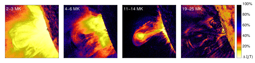
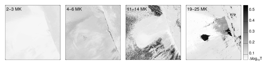
Figure 4: Maps of the (top row) vertical uncertainty $\Delta\xi(T)$ and (bottom row) horizontal uncertainty, or temperature resolution $\Delta\log{T}$, in the regularized DEM solution shown in Figure 3 for four temperature ranges.

To get a better understanding of the spatial structure of the event we can create DEM maps for each temperature range, shown in Figure 3. Many pixel locations in these maps show emission across a broad range of temperatures, highlighting the complex, multi-thermal nature of the line-of-sight DEMs. The temperature maps for 0.5-1MK and 8-11MK do resemble the images from the 171Å and 131Å channels respectively showing that the emission here is mostly from one component of the channels’ response. However for the other temperature maps, features start to appear that are not apparent in the SDO/AIA images themselves, such as there being little 4-6MK emission about the core of the erupting plasmoid. This emphasizes the complicated temperature response of SDO/AIA filters and the necessity of the DEM inference to interpret the temperature or density structures in the corona. Before discussing these spatial properties it is prudent to investigate which of the regularized DEMs are robust solutions.

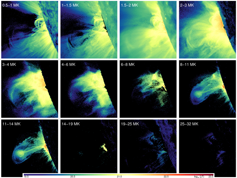
Figure 5: DEM maps in different temperature ranges for the 3-Nov-2010 flare at 12:15:02 as shown in Figure 3 but only showing pixels where $\Delta\xi(T)\leq 30\%$ and $\Delta\log{T}\leq 0.25$. The colour scale is $\log{\xi(T)}$ and is in units of cm^-5K^-1.

One major advantage of our regularization approach is that it produces information about the vertical $\Delta\xi(T)$ and horizontal $\Delta\log{T}$ uncertainty in the regularized solution (see §2.2) and so we can plot uncertainty maps, shown in Figure 4. The vertical error $\Delta\xi(T)$ (top row, given as a percentage error of the DEM signal) show the largest uncertainties are predominantly from the regions where the emission measure is very low as well as at the highest temperatures. The latter is due to a combination of SDO/AIA having lower sensitivity to the temperatures $>20$MK and there also being little plasma emitting in this temperature range. Hence the data, and also DEM, are very noisy. Conversely, at the temperatures where SDO/AIA has a very strong response (about 0.5 to 3MK) and there is bright solar emission, the signal, and hence DEM, has a very small associated vertical error.

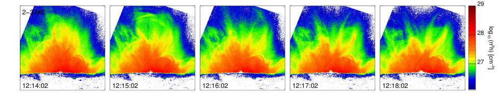
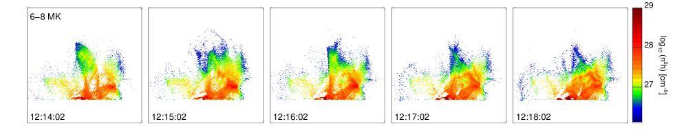
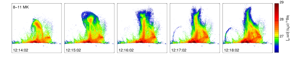
Figure 6: Emission Measure maps for various times in 2-3MK, 6-8MK and 8-11MK (top, middle, bottom rows). These maps have been rotated by $110^{\circ}$. The second column is of the time interval shown in previous Figures. A movie of this is available with the electronic version of this paper, covering the 1-1.5 to 14-19MK from 12:12:02 UT to 12:19:52 UT, see Figure 13.

The horizontal error in the solution (bottom row Figure 4) are mostly slightly larger than the SDO/AIA minimum theoretical limit of temperature resolution $\Delta\log{T}=0.1$ (Judge 2010). The largest uncertainties again come from regions where there is a weak signal and/or noisy data, this is particularly evident for the largest temperatures. But there are are also positions where the data is noisy in the hottest temperature bands yet the horizontal error is small. This is due to the regularization approach robustly determining that there is very weak/no emission at these positions and temperature. Where the horizontal errors (temperature resolution) are small it means that the emission is confined to that temperature range but with large errors ($\geq 0.3$) it suggests the emission shown in that temperature band could actually be attributed to a neighbouring temperature bins. Therefore at temperatures where the horizontal uncertainty are large the DEM solution should be treated with caution (see Hannah & Kontar 2012) and additional analysis of the residuals could be useful (e.g. Piana et al. 2003).

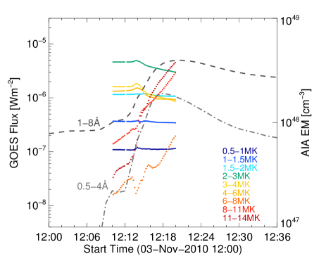
Figure 7: GOES SXR lightcurve of the 3-Nov-2010 flare C4.9 (grey lines) with the spatially integrated emission measures derived from the SDO/AIA observations for the chosen temperature ranges (colored lines).

Using this error information we can restrict the DEM maps to only show the values with the smallest vertical and horizontal errors and this is shown for $\Delta\xi(T)\leq 30\%$ and $\Delta\log{T}\leq 0.25$ in Figure 5. At the hottest temperature (25-32MK) there is virtually no emission due to the largest uncertainties and poor confidence in the DEM solution and any weak emission shown is likely unreliable. In 14-19MK the emission is predominantly coming from the flare heated material that has risen above the limb though there is a hint of very faint emission from the plasmoid core. These loops show the strongest emission in 8-11 and 11-14MK but also in these temperature ranges is the plasmoid core, an envelope of surrounding material and the filamentary stem behind it, all sharply visible. The plasmoid core has slightly stronger emission in 11-14MK than 8-11MK. Only a single thin stem structure is clearly defined in 11-14MK but two, in a V-shape diverging away from the plasmoid core, are visible in 8-11MK. In both cases their high temperatures, and the inflow region to these stems, is not explained by the classical flux rope eruption model. Some additional heating maybe present and the Kelvin-Helmholtz waves to the top of the erupting material are a signature of a reconnection layer surrounding the erupting flux rope, producing a secondary means of releasing energy (Foullon et al. 2011, 2012).

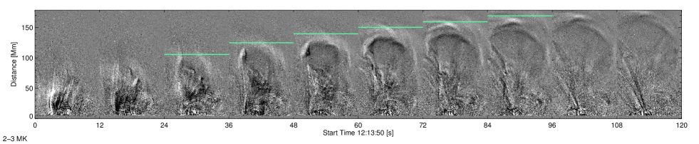
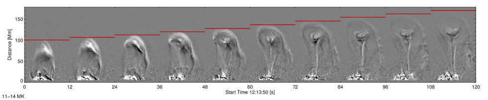
Figure 8: Running differences of the DEM maps ($\xi(T,x,y,t_{i})-\xi(T,x,y,t_{i-1})$) for 2-3MK (top row) and 11-14MK (bottom row). The leading edge of the erupting plasma was tracked and is indicated by the red horizontal lines The resulting height profiles as a function of time for these and other temperature ranges is shown in Figure 9 and 10. These maps have been rotated by $110^{\circ}$.

At cooler temperatures ($\leq$6MK) the core of the plasmoid disappears, which is likely the cause of the dimming observed in some SDO/AIA images but it is not clear whether this is due to heating or mass loss. To try and understand this we look at the time evolution of the maps in §3.4. The V-shaped structure of the stems is still present though, clearly in 6-8MK but slightly obscured by the bright surrounding coronal emission in 3-4 and 4-6MK. Ahead of the plasmoid core we start to see the leading edge of a front of material, visible in 2-3, 3-4 and 4-6MK. This density increase of material is likely due to a compression front being driven ahead of the erupting plasmoid. At the coolest temperatures (0.5-1, 1-1.5 and 1.5-2MK) there is some faint evidence of the leading edge moving out but it is dominated by the emission from several hot coronal loops associated with the occulted active region and flare.

3.4 Time Evolution

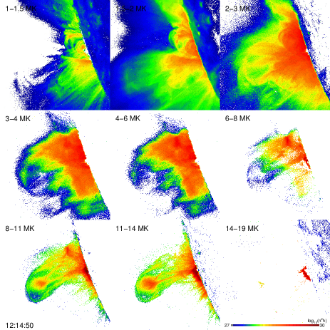
Figure 13: One frame of the movie, available online, showing the EM maps, $\log{n^{2}h}$ in units of cm^-5, for the temperature ranges 1-1.5 through to 14-19MK, starting at 12:12:02 UT running till 12:19:52 UT.

As the 03-Nov-2010 solar eruption is highly dynamic we investigate the DEM maps as a function of time, which we have shown in three temperature ranges at 1 minute intervals in Figure 6. A movie of this is available with the electronic version of this paper, covering 1-1.5 to 14-19MK from 12:12:02 UT to 12:19:52 UT, see Figure 13. We have also converted the DEM maps into EM maps by removing the factor $\ln{10}T\mathrm{d}\log{T}$, resulting in the values shown being $EM=n^{2}h$ [cm^-5], making it easier to calculate densities (see §3.5). Again we have only shown the emission in the pixels and temperature ranges that have $\Delta\xi(T)\leq 30\%$ and $\Delta\log{T}\leq 0.25$, as in Figure 5.

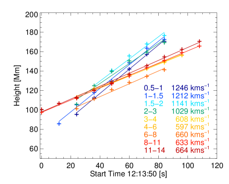
Figure 9: Height (above an arbitrary origin) versus time profiles of the leading edge of the erupting plasma for each of the temperature ranges the propagation could be reliably tracked.

In the 2-3MK temperature range (top row Figure 6) we see the leading edge of the eruption clearly at 12:15:02 UT but afterwards gone and the loops bending/collapsing back. There is some strong emission ahead of erupting flux rope at 12:14:02 UT but that disappears at later times, likely erupted. Lower in the corona the loops barely change over time and only the highest ones modify, being bent back after the eruption, leaving a void where the stem forms in higher temperatures. In 6-8MK (middle row Figure 6) we see the initial eruption of the plasmoid core and stems behind it at 12:14:02 UT but at later times there is a void of material at this temperature, again suggestive of material loss (or spreading out) due to the eruption mass loss. There is increased emission from the loops that have bundled up below the eruption to the right indicating possible heating of material in these contracting loops.

The erupting plasmoid and the filamentary stem structure connecting it to the lower solar atmosphere is sharply defined in 8-11MK (bottom row Figure 6). The strong emission from the core of the plasmoid quickly weakens as it moves higher leaving the strongest emission from the vertical stem behind it. It would be tempting to immediately classify this structure as a current sheet, given the superficial similarity to the classical eruption model. However this stem is relatively thick and appears to be made up of several thinner structures. This maybe a projection effect with multiple thin stem misaligned along the line-of-sight. A bigger issue is that this structure shows strong emission in this hot (11-14MK) temperature range and again the classical model is unable to explain the presence of such hot material inflowing to the current sheet. Below to the right of the eruption (or to the top right in the original orientation) hot loops bundle up between 12:16:02 UT to 12:18:02 UT. This is associated with Kelvin-Helmholtz waves (Foullon et al. 2011) and possible density increases due to outflowing material (Savage et al. 2012). In the classic eruptive model this region would be associated with shrinking loops and the outflow from the reconnection region. However the dynamics here are clearly more complicated and difficult to unambiguously ascertain due to the strong emission lower in the atmosphere. In the 12:17:02 UT and 12:18:02 UT images another large coronal loop develops to the left of the main eruption. This fainter emission in 11-14MK is likely flare heated material that has expanded into this large loop. STEREO-B/SECCHI images from behind the limb do show a separate core flaring region located at the base of this hot loop (Savage et al. 2012).

By summing over the whole of the region shown in Figure 6 we can produce a time profile in each temperature band, shown in Figure 7 in comparison to the GOES SXR emission. We have computed this between 12:12:02 UT and 12:19:50UT (the time range shown in the movie available in the electronic version of this paper, see Figure 13) as saturation from the flaring loops starts to dominate and produces unreliable EM maps in these regions. From Figure 7 we see that there is a slight increase in most of the temperature ranges as the eruption begins (12:13UT) which then drops off as the material is ejected (12:15UT), suggesting this initial change is due to the heating, then the loss of coronal plasma. After this the hottest temperature ranges (6-8, 8-11 and 11-14MK) increase in a similar manner (though slightly delayed) to the SXR emission observed by GOES. This is initially due to further heating in the current sheet and the shrinkage of loops below the eruption with heated material outflowing the reconnection region. The later sharp increase is likely due to the bright post-flare loops rising above the limb. At the cooler temperatures it will be later in the event before the current sheet and flare heated material (if visible above the limb) cool into these temperature range. This explains the decrease in the emission at these temperatures after the loss of material during the eruption. The very small decrease at the smallest temperatures (0.5-1, 1-1.5, 1.5-2MK) suggest that this emission is dominated by the background and line-of-sight coronal emission over the whole region.

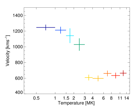
Figure 10: Velocity of the leading edge of the eruption as a function of temperature, obtained from linear fits to the data shown in Figure 9. The vertical uncertainty is taken as the largest of the error in the parameter from the linear fits shown in Figure 9 and three AIA pixels travelled in 12s.

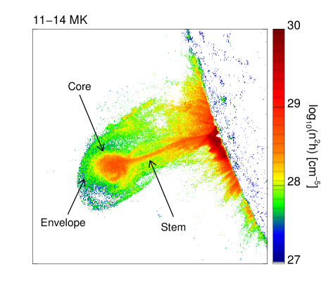
Figure 11: Emission Measure map for 11-14MK at 12:15:02 UT with the different components identified.

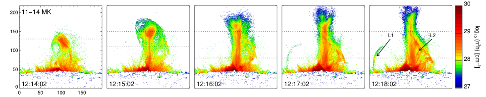
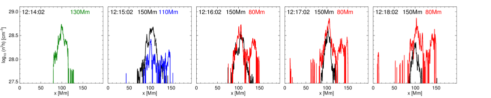
Figure 12: (Top) Emission Measure maps for various times in 11-14 MK. (Bottom) The emission measure profile at various heights for one minute time intervals in 11-14 MK, indicated by the dotted lines in the top panel.

To investigate the time profile of the erupting material in different temperature ranges we have manually tracked the front of the emission in running difference maps of the emission measure, i.e. $\xi(T,x,y,t_{i})-\xi(T,x,y,t_{i-1})$. This is shown in Figure 8 for 2-3 and 11-14MK, with black indicating a decrease in emission, white an increase and the colour lines showing the manually tracked front of the eruption. This type of analysis has been performed before but in individual SDO/AIA wavelength channels (Cheng et al. 2011; Bain et al. 2012) and not for specific temperature ranges. The former has the advantage of a clearer time evolution as the channels are a $\approx$3s duration image every 12s whereas the EM maps are effectively 12s cadence due to the use of six different channels in their calculation. This makes the determination of the leading edge tricky and the resulting height (above an arbitrary position) as a function of time for the different temperature ranges are shown in Figure 9. Here we have linearly fitted the data to produce a velocity as a function of temperature. These velocities and there associated error (the largest between the error in the fitted parameter and from three SDO/AIA pixels travelled in 12s) are shown in Figure 10. In the cooler temperature range the leading edge of the eruption travels at 1 246 kms^-1 in 0.5-1MK decreasing to 1 029 kms^-1 in 2-3MK. This general trend of a slower eruption at higher temperature is more evident above 3-4MK once we are in the range associated with the plasmoid eruption itself. From 3-4Mk to 11-14MK the velocities are consistently between 597 kms^-1 to 664 kms^-1 suggesting the multi-thermal structure is moving outwards together. These two distinct structures at different velocities are consistent with those found by tracking the eruption in the SDO/AIA channels (Cheng et al. 2011; Bain et al. 2012), with the 131Å  and 335Å  at 667 and 747 kms^-1 and the cooler 211Å and 193Å at 1 154 and 1 439 kms^-1 (Bain et al. 2012).

Table 1: Thermal parameters for the different features shown in Figures 11 and 12.

					(h=w)		Energy		(h=100Mm)	Energy
Time	Feature	EM	Width	Length	Density	Vol	Thermal	Kinetic	Density	Thermal	Kinetic
		$10^{28}$cm-5	Mm	Mm	$10^{9}$cm-3	$10^{28}$cm3	$10^{29}$erg	$10^{29}$erg	$10^{9}$cm-3	$10^{29}$erg	$10^{29}$erg
12:14:02	Core	$2.5$	25	40	$3.2$	2.5	$4.1$	2.9	1.6	8.2	5.8
12:15:02	Core	$3.9$	30	30	$3.6$	2.7	$5.1$	3.6	2.0	9.3	6.5
	Envelope	$0.5$	65	100	$0.9$	39.6	$18.0$	12.6	0.7	23.8	16.7
	Stem	$2.5$	7	80	$6.0$	0.4	$1.2$		1.6	4.6
12:16:02	Stem	$2.0$	25	100	$2.8$	6.3	$9.1$		1.4	18.3
12:17:02	Stem	$3.2$	20	110	$4.0$	4.4	$9.1$		1.8	20.3
12:18:02	Stem	$1.6$	10	130	$4.0$	1.3	$2.7$		1.3	8.5

3.5 Density and Thermal Energy

To recover the density from the EM maps an estimate of the line-of-sight depth $h$ of the emission is required. As the structures are sharply defined at higher temperatures (visbile in Figure 11, labelling the three distinct components: plasmoid core, envelope and stem) we can use their apparent width in the EM maps as the depth assuming spherical/cylindrical symmetry. We focus just on 11-14MK here as the structures are similar in shape to those in 8-11MK (bottom row of Figure 6) and at lower temperatures this would be difficult as the shape of the structures is far harder to estimate reliably. The density of the sheath of the Kelvin-Helmholtz waves has been estimated at lower temperatures (about 4MK) using emission measures found using both our regularized approach and Gaussian model forward-fitting techniques, finding similar values, and is the subject of a separate publication (Foullon et al. 2012).

The EM maps in 11-14MK for 5 time intervals during the plasmoid eruption are shown in Figure 12 (top row). Here we have plotted the EM as a function of position (bottom row) for various slices through the erupting structure, indicated in the EM maps by dotted horizontal lines. From these slices we can determine a width of the structures of interest: the erupting plasmoid core, envelope and stem. Assuming a spherical/cylindrical geometry in these structure we can use the width as the depth, giving the line-of-sight extent $h$. Since $EM=n^{2}h$ this readily gives an estimate of the density in the structure and these values for the various structures at the different times are given in Table 1. Here we see that the density in the core region (about $3\times 10^{9}$cm^-3) does not change between the two time intervals shown before it fully erupts. The envelope of material surrounding the plasmoid core has a lower density ($3\times 10^{8}$cm^-3) but still shows a sharp transition to the background corona as that has effectively no emission in this temperature range.

The density in the stem region does decrease over time but that is initially due to a widening of the structure (seen at 12:16:02 UT onwards) rather than a reduction in the emission measure. As discussed before, it is difficult to attribute such a wide hot structure to the monolithic current sheet as proposed by the classic eruption model. If we instead assuming the structures are more elongated, using a line-of-sight component of $h=100$Mm (shown in Table 1), we find that the density of the stem does not vary much with time. In fact these slightly smaller densities (about $10^{9}$cm^-3) are fairly similar for both the core and stem regions.

The thermal energy of this emission can be calculated via $W_{\mathrm{T}}=3nVk_{\mathrm{B}}T$, where we take $T=12.5$MK the middle of the temperature range. We estimate the volume using $V=whL$, with $w$ the width, $h$ the line-of-sight component and $L$ the extent perpendicular in the image to $w$. This is found using a filling factor of unity, and as this could be smaller, the values we calculate are upper limits to the thermal energy. Note that for the envelope region we have calculated the volume of the region minus the volume of the plasmoid core. The energies are shown in Table 1 for the times and regions in Figure 12. We find that the thermal energy in this temperature range as the core erupts increases slightly ($4.1$ to $5.1\times 10^{29}$ erg) whereas the energy in the stem structure greatly increases just after the impulsive eruption ($1.2$ to $9.1\times 10^{29}$ erg). This is due to the widening of the stem whilst maintaining the same emission measure per pixel within the stem. This weakens by 12:18:02 UT when the emission measure starts to drop and the stem narrows. If we again assume the structures are elongated, with line-of-sight $h=100$Mm, we get a smaller variation between the thermal energy of the different structures and how they evolve with time, with energies of about $10^{30}$ erg. In both cases there is an increase in the thermal energy of the stem which is consistent with the idea of continuous energy release in this region. The envelope of hot material around the plasmoid core has a considerably higher thermal energy but that is because it is larger structure.

We can also calculate the kinetic energy for the structures which clearly propagate outwards, the plasmoid envelope and core. The kinetic energy is taken as $W_{\mathrm{K}}=nVm_{\mathrm{p}}v^{2}/2$ where $m_{\mathrm{p}}$ is the proton mass and the velocity is $v=660$ kms^-1 from Figure 9. These are again given in Table 1 for $h=w$ and $h=100$Mm. Here we find that the thermal energy (in 11-14MK) is consistently slightly larger than the kinetic energy of the material in this temperature range. A higher thermal to kinetic energy was also found previously by Landi et al. (2010). This similarity between the thermal and kinetic energies is typical for CMEs from observations higher in the corona (e.g. Forbes 2000). Our values for the energies are also smaller than those for a “moderately” large CME (Forbes 2000) ($10^{30}$ versus $10^{32}$ erg) which is expected as our energy is just from one component of the CME and in one temperature range.

3.5.1 Coronal Loop Density

In the later time intervals in Figure 12 (12:18:02 UT) there are distinctive coronal loops associated with the flaring region (L1) and the shrinkage below the eruption (L2). Again assuming $w=h$ we can calculate the loop density, taking them to be about 2Mm, though we do not estimate the energy as we cannot determine a reliable loop length. The large coronal loop (L1), associated with the core of the occulted flaring region, is visible from 12:17:02 UT onwards, and its density increases as more hot material fills the loop (from $5.6\times 10^{9}$cm^-3 to $7.1\times 10^{9}$cm^-3). The loops below the ejected material (L2) have an emission measure that doubles between 12:17:02 UT and 12:18:02 UT, resulting in a density increase to $1.3\times 10^{10}$cm^-3 from $8.9\times 10^{9}$cm^-3. This increase in heated material maybe due to outflows from the reconnection region in the stem structure (Savage et al. 2012) or the reconnection layer above the loops where Kelvin-Helmholtz waves were located (Foullon et al. 2012).

4 Discussion & Conclusions

Regularized inversion of multi-filter observations provides an essential tool to study the temporal and spatial evolution of multi-thermal plasma during eruptive events. The regularized maps of an erupting CME presented in the paper allow the basic plasma properties (integrated along the line-of-sight) to be inferred and calculation of the density and energetics of various parts of the eruption. We find that the leading edge of the eruption travels between 1 029-1 246 km s^-1 and has the temperature range $\leq$2-3MK followed by slower 597-664 km s^-1 but hotter plasma $\geq$3-4MK. The erupting core and stem which could be interpreted as a plasmoid with a current sheet appears sharply defined in 11-14MK. The width of the stem/current sheet we find (7-25Mm) is far larger than that expected in the classical reconnection model, and somewhat smaller than the predicted $<1Mm$ (Vršnak et al. 2009). This value is in fact smaller than those found higher in the corona (e.g. Ciaravella et al. 2002; Landi et al. 2012) suggesting continuous expansions as the CME lifts up. The stem/current sheet width we determine is however at a higher temperature range and made with a higher spatial resolution observations than these previous results.

During the impulsive phase, we find that the density is about $3\times 10^{9}$ cm^-3, $6\times 10^{9}$ cm^-3, $9\times 10^{8}$ cm^-3 in the plasmoid core, stem and surrounding envelope of material. This gives thermal energy estimates of $5\times 10^{29}$ erg, $1\times 10^{29}$ erg and $2\times 10^{30}$ erg. These are slightly larger than the values found for the kinetic energy of the erupting envelope and core, which is consistent with previous CME energy estimations (Landi et al. 2010). The observations also show the increase of the thermal energy of the core (plasmoid) and of the stem (current sheet) as the CME is rising from 12:14:02 UT to 12:17:02 UT, suggesting ongoing energy release. The increase of energy is more noticeable for the stem with it more than doubling over 3 minutes. This is consistent with the predictions of recent reconnection models (Murphy et al. 2010; Reeves et al. 2010, e.g.) with the energy released in the current sheet pumped into the plasmoid.

The reconstructed DEM maps show the multi-thermal nature of the corona, which is unsurprising given that we have a hot plasmoid erupting through the cooler surrounding corona, two distinct structures with different temperature characteristics. Our DEM maps show in greater detail the same basic physical picture that was found by Cheng et al. (2012) using a different DEM reconstruction method for a few regions in the CME. Namely that the bright leading front of the CME is composed of a corona-like temperature distribution, with the increased emission due to the accumulation of material, whereas the erupting core contains heated material ($>8$MK). All DEM solutions however should be treated carefully given the uncertainties in the temperature response functions and the possibly broad temperature resolution (Testa et al. 2012). Used carefully, with these issues kept in mind, regularized DEM maps present a useful tool for exploring the dynamics of heating in the solar corona with SDO/AIA observations.

Appendix A EM Movie of the Eruption