The Impact of Helium-Burning Reaction Rates on Massive Star Evolution and Nucleosynthesis

Abstract

We study the sensitivity of presupernova evolution and supernova nucleosynthesis yields of massive stars to variations of the helium-burning reaction rates within the range of their uncertainties. The current solar abundances from Lodders (2009) are used for the initial stellar composition. We compute a grid of 12 initial stellar masses and 176 models per stellar mass to explore the effects of independently varying the ${}^{\text{12}}$C($\alpha,\gamma$)${}^{\text{16}}$O and 3$\alpha$ reaction rates, denoted $R_{\alpha,12}$ and $R_{3\alpha}$, respectively. The production factors of both the intermediate-mass elements (A=16-40) and the s-only isotopes along the weak s-process path (⁷⁰Ge, ⁷⁶Se, ⁸⁰Kr, ⁸²Kr, ⁸⁶Sr, and ⁸⁷Sr) were found to be in reasonable agreement with predictions for variations of $R_{3\alpha}$ and $R_{\alpha,12}$ of $\pm 25\,\%$; the s-only isotopes, however, tend to favor higher values of $R_{3\alpha}$ than the intermediate-mass isotopes. The experimental uncertainty (one standard deviation) in $R_{3\alpha}$($R_{\alpha,12}$) is approximately $\pm 10\,\%$($\pm 25\,\%$). The results show that a more accurate measurement of one of these rates would decrease the uncertainty in the other as inferred from the present calculations. We also observe sharp changes in production factors and standard deviations for small changes in the reaction rates, due to differences in the convection structure of the star. The compactness parameter was used to assess which models would likely explode as successful supernovae, and hence contribute explosive nucleosynthesis yields. We also provide the approximate remnant masses for each model and the carbon mass fractions at the end of core-helium burning as a key parameter for later evolution stages.

1 Introduction

Massive stars are responsible for the production of most intermediate-mass ($\mathrm{A}=16-40$) isotopes through hydrostatic burning phases and subsequent supernovae (Burbidge et al., 1957; Woosley et al., 2002). During core-He burning the ${}^{\text{12}}$C($\alpha,\gamma$)${}^{\text{16}}$O and 3$\alpha$ reactions compete to determine the relative abundances of oxygen and carbon prior to core-C burning. Changes in these abundances have significant effects on subsequent stellar evolution and structure and on the resulting nucleosynthesis. The carbon abundance influences subsequent shell burning episodes and affects whether core-C burning will be radiative or convective. There is also a non-monotonic relation between the carbon abundance and the resulting remnant mass (Woosley et al., 2003), so that these reactions are important for understanding the populations of neutron stars (NS) and black holes (BH).

These rates can also affect weak s-process yields. The weak s-process is a slow neutron capture process occurring at the end of convective core-He burning and during shell carbon burning (Pignatari et al., 2010), and contributes to isotopic production along the s-process path above iron and up to a mass number of A$\approx$100 (Raiteri et al., 1993). A change in the helium-burning rates can induce a corresponding change in temperature to keep the star at constant luminosity, and the reaction for the neutron source for the weak s-process, ${}^{\text{22}}$Ne($\alpha,\mathrm{n}$)${}^{\text{25}}$Mg, is highly temperature-dependent. Additionally, the amounts of neutron poisons have been shown to vary with these rates (Rayet and Hashimoto, 2000; Tur et al., 2009).

Although not discussed in this paper the production of the important radioactive nuclei ²⁶Al, ⁴⁴Ti, and ⁶⁰Fe (Tur et al., 2010) is also sensitive to these rates. Gamma rays from these nuclei provide observational information that may help to test models of massive star internal structure and nucleosynthesis through the constraints imposed by the abundance ratios of $\mathrm{{}^{44}\mathrm{Ti}/^{56}Co}$ and $\mathrm{{}^{26}Al/^{60}Fe}$ (Diehl et al., 2006; Leising and Diehl, 2009).

This work is an extension of the study by Tur et al. (2007, 2009), who calculated a limited subset of models of our full 2D parameter space. They concluded that across the 2$\sigma$ uncertainty range root-mean-square (rms) deviations for the production factors sometimes vary non-monotonically with the rates, as do deviations in the remnant mass, indicating that both helium burning reactions are independently important (Tur et al., 2007). We extend upon their study by performing a much finer sampling of the 2$\sigma$ uncertainty range to assess the effect of changing the rates independently, in order to map the whole 2D landscape to determine the true non-monotonic behavior with a higher resolution grid. The purpose is to: i) examine the effect of varying the helium burning reaction rates on the production factors of intermediate-mass isotopes, ii) examine the effect on the production factors of the six s-only isotopes along the weak s-process path, iii) assess the impact on i) and ii) of including only models that are likely to explode as successful supernovae, and iv) examine the effect on the remnant mass. We do not address the effect of varying the solar abundance set, which indeed has been shown to impact the final nucleosynthesis, and is studied in Tur et al. (2007) for the intermediate-mass isotopes and in Tur et al. (2009) for the weak s-process isotopes. We use an updated solar abundance set (Lodders, 2009) that was not yet available for the previous studies. It was corrected for the weak s-only isotopes by subtracting estimated main s-process contributions, as described in Section 2. We note that recent 3-body calculations of the 3$\alpha$ reaction show an increase in this rate at temperatures below $\sim 0.07\,\mathrm{GK}$ (Nguyen et al., 2012). This will not impact the current study as He ignition in massive stars occurs beyond this threshold, at $T_{3\alpha}\sim 0.1\,\mathrm{GK}$.

This paper has the following outline: in Section 2 we describe the stellar models and methods used in the analysis. In Section 3 we compare the intermediate-mass and weak s-process isotopes across all models, and for the subset of models likely to explode as supernovae rather than collapse to black holes (we ignore hypernovae and gamma ray bursts). This subset is chosen using a compactness parameter filter. We also discuss the remnant mass and carbon mass fractions at the end of core-He burning for the different stellar masses. Our conclusions are given in Section 4.

2 Stellar Models and Analysis

All models were computed using KEPLER, a time-implicit one-dimensional hydrodynamics package for stellar evolution (Weaver et al., 1978; Rauscher et al., 2002). A grid of 12 initial stellar masses M/$\mathrm{M}_{\text{$\odot$}}$=12, 13, 14, 15, 16, 17, 18, 20, 22, 25, 27, and 30 was used, with the revised pre-solar abundances from Lodders (2009) for the initial composition. For each stellar mass, 176 models were computed to scan at least a 2$\sigma$ uncertainty range for both the ${}^{\text{12}}$C($\alpha,\gamma$)${}^{\text{16}}$O and 3$\alpha$ reaction rates, denoted $R_{\alpha,12}$ and $R_{3\alpha}$, respectively. This range was parametrized as a multiplier on the centroid values for the rates, as done by Tur et al. (2007). The centroid values used in KEPLER are taken from Caughlan and Fowler (1988) for $R_{3\alpha}$, and 1.2 times the rate recommended by Buchmann (2000) for $R_{\alpha,12}$. The range for the $R_{\alpha,12}$ multipliers was $\left(0.5,2.0\right)$ with a resolution of $\Delta=0.1$, and the range for the $R_{3\alpha}$ multipliers was $\left(0.75,1.25\right)$ with a resolution of $\Delta=0.05$. Commonly accepted uncertainties for $R_{3\alpha}$ and $R_{\alpha,12}$ are $\pm 10\,\%$ (Chernykh et al., 2010) and $\pm 25\,\%$. Our total range was, conservatively, slightly more than $\pm 2\sigma$.

In Fig. 2 we show the grid of models computed both by Tur et al. (2007) and in the present work.

The $R_{\alpha,12}$ and $R_{3\alpha}$ reaction rate multiplier values used in the stellar models. The models using the reaction rate multiplier pairs given in red plusses, green asterisks, and blue squares were performed by Tur et al. (2007). The black asterisks show the models computed in the present work.

All stellar models were first evolved through hydrostatic burning until the Fe core collapsed, and an inward velocity of $10^{8}\,\mathrm{cm\,s^{-1}}$ was reached. The explosion mechanism for the resulting supernova was modeled as a mechanical piston that imparted an acceleration at constant Lagrangian mass coordinate to provide the desired total kinetic energy of the ejecta, taken in these models to be 1.2 B ($\mathrm{1\,B}=10^{51}\,\mathrm{erg}$) at 1 year after the explosion. For details on the parametrization of the explosion used in KEPLER see Woosley and Heger (2007), and references therein. For details on the treatment of convection and mixing see Woosley and Weaver (1998) and Woosley et al. (2002), and a discussion of the mass cut is given in Tur et al. (2007) and Heger and Woosley (2010). Effects of rotation and magnetic fields are ignored. The final supernova yields for all models were then averaged by integrating over the Salpeter initial mass function (IMF) for each reaction rate multiplier pair in Fig. 2. The yields from stellar winds were included.

$$Y_{i}^{*}=\sum_{j}\intop_{m_{j}}^{m_{j+1}}\xi\left(m\right)\cdot\left(s_{i,j}\cdot\left[m-m_{j}\right]+Y_{i,j}\right)\cdot dm$$ (1)

$$P_{i}=\frac{Y_{i}^{*}}{X_{i,\odot}\cdot\sum_{k}Y_{k}^{*}}$$ (2)

In Equation 1 the IMF interpolated yield mass for isotope i is given by $Y_{i}^{*}$, and the Salpeter mass spectrum is $\xi\left(m\right)=C\cdot m^{-2.35}$, where $C$ is the proportionality constant . The mass grid used for the integrations are the ejected masses, defined as the baryonic remnant masses subtracted from the initial stellar mass grid. Yields are linearly interpolated between adjacent masses in the integral, with the slope defined by, $s_{i,j}=\left(Y_{i,j+1}-Y_{i,j}\right)/\left(m_{j+1}-m_{j}\right)$, where $Y_{i,j}$ is the yield mass of isotope i from a model with initial mass $m_{j}$. In Equation 2 the production factor for isotope i is given by $P_{i}$, the sum in the denominator runs over all isotopes, and the solar mass fraction of isotope i is given by $X_{i,\odot}$.

Massive stars are responsible for producing nearly the entire solar abundance of a subset of intermediate-mass isotopes, namely ^16,18O, ²⁰Ne, ²³Na, ²⁴Mg, ²⁷Al, ²⁸Si, ³²S, ³⁶Ar, and ⁴⁰Ca. Hence, in order to make the solar abundance pattern, massive near-solar metallicity stars need to produce these intermediate-mass isotopes in solar ratios. An analysis of the standard deviations of the production factors for this set of isotopes is used in the present work to identify helium reaction rate values that agree with solar observations. This agreement is an approximation that the above isotopes owe their entire solar abundance to massive, near-solar metallicity stars, and relies on sufficient sampling of the initial mass function (IMF) and understanding of the initial compositions. As mentioned, the impact of uncertainties in the initial composition is not addressed in this work, but an analysis of the effect of different compositions can be found in Tur et al. (2007).

For the weak s-process isotopes a correction is necessary, since the solar abundances of the six s-only isotopes along the weak s-process path (⁷⁰Ge, ⁷⁶Se, ⁸⁰Kr, ⁸²Kr, ⁸⁶Sr, and ⁸⁷Sr) have additional contributions from the main s-process, which occurs in asymptotic giant branch (AGB) stars, not massive stars. Hence what is needed are the production factors relative to the contributions from the weak s-process only, not relative to the entire solar abundance. To achieve this, the solar abundance decomposition from West and Heger (2012) was used, which gives, in part, the approximate solar contributions for the six weak s-only isotopes. This modifies Equation 1. with the substitution of $X_{i,w}$ for $X_{i,\odot}$, where $X_{i,w}$ denotes the contribution to the solar mass fraction of isotope i from the weak s-process.

3 Results and Discussion

3.1 Comparison of ${}^{\text{12}}$C($\alpha,\gamma$)${}^{\text{16}}$O and 3$\alpha$ Reaction Rates

The production factors for the models were computed using Equations 1 and 2, and standard deviations were calculated for each model, using the intermediate-mass isotope set (in Section 4.1) and the six s-only isotopes along the weak s-process path (in Section 4.2),

$$\sigma_{P}=\sqrt{\frac{\sum_{k=1}^{n}P{}_{k}^{2}}{n-1}-\left(\frac{\sum_{k=1}^{n}P{}_{k}}{n-1}\right)^{2}}$$ (3)

where $P{}_{k}$ are the production factors computed in Equation 2, and $n$ is the number of entries in the isotope list: 10 for the intermediate-mass isotopes and 6 for the s-only isotopes along the weak s-process path. We distinguish $\sigma_{P}$ (the standard deviation of the production factors) from $\sigma$ (the uncertainty in the rates). Since massive stars contribute to most of the solar abundances for the intermediate-mass isotopes considered (or a fraction of them in the case of the s-only isotopes), low standard deviations should indicate combinations of $R_{\alpha,12}$ and $R_{3\alpha}$ that agree with observations. We first follow the type of analysis performed by Tur et al. (2007), for constant $R_{\alpha,12}$ and $R_{3\alpha}$ multipliers, shown in Fig. 1.

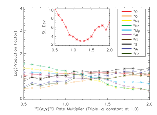
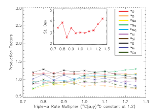
Figure 1: Left: The production factors for the intermediate-mass isotopes averaged over the IMF as a function of the $R_{\alpha,12}$ multiplier, at a constant $R_{3\alpha}$ multiplier of 1.0. Right: The production factors for the intermediate-mass isotopes averaged over the IMF as a function of the $R_{3\alpha}$ multiplier, at a constant $R_{\alpha,12}$ multiplier of 1.2. The inset graph shows the standard deviations.

For a constant $R_{3\alpha}$ multiplier of 1.0 (Fig. 1, left), values for the $R_{\alpha,12}$ multiplier are favored within about $\pm$25 % of the centroid multiplier of 1.2. For a constant $R_{\alpha,12}$ multiplier of 1.2 (Fig. 1, right), values for the $R_{3\alpha}$ multiplier have a minimum standard deviation at 0.85, and vary across a similar range of standard deviation values for a $\pm 25\,\%$ change in $R_{3\alpha}$. Since $R_{3\alpha}$ is better experimentally determined, however, the extremes of this range are less likely than for $R_{\alpha,12}$. The results in Fig. 1 show approximate qualitative agreement with the findings of Tur et al. (2007), but care must be taken in a comparison as they do not use the Lodders (2009) abundances, and they have demonstrated that there is non-trivial variation among different solar abundance sets.

The corresponding plot for the weak s-only isotopes is given in Fig. 2.

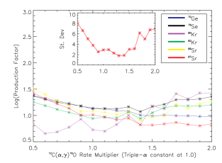
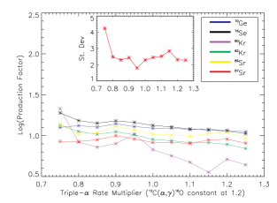
Figure 2: Left: The production factors for the weak s-only isotopes averaged over the IMF as a function of the $R_{\alpha,12}$ multiplier, at a constant $R_{3\alpha}$ multiplier of 1.0. Right: The production factors for the weak s-only isotopes averaged over the IMF as a function of the $R_{3\alpha}$ multiplier, at a constant $R_{\alpha,12}$ multiplier of 1.2. The inset graph shows the standard deviations.

For a constant $R_{3\alpha}$ multiplier of 1.0 (Fig. 2, left), values for the $R_{\alpha,12}$ multiplier have a minimum standard deviation at 1.3. For a constant $R_{\alpha,12}$ multiplier of 1.2 (Fig. 2, right), the standard deviation has a minimum at the $R_{3\alpha}$ multiplier value of 0.95. Significant variations in the production factors exists across both multiplier ranges.

3.2 Intermediate-Mass Isotopes

To address how changing the rate multipliers independently affects the nucleosynthesis, the entire set of models in $\left(R_{\alpha,12},R_{3\alpha}\right)$ space was mapped in a 2D grid, rather than restricting ourselves to 1D slices. Results are first given for just the 25 $\mathrm{M}_{\text{$\odot$}}$ models (Fig. 3.2). The corresponding plots for all models can be found in the Appendix.

Standard deviations of the production factors as a function of the $R_{\alpha,12}$ and $R_{3\alpha}$ reaction rate multipliers for the 25 $\mathrm{M}_{\text{$\odot$}}$ models. Each model is given by the $R_{\alpha,12}$ and $R_{3\alpha}$ reaction rate multiplier pair used for the helium rates.

The best fit $R_{\alpha,12}$ and $R_{3\alpha}$ values occupy a region in the lower right-hand corner, and a strip running approximately though the centroid value for each rate. It is interesting that some adjacent models display significant differences in their nucleosynthesis despite small change in the reaction rate multipliers, for example $\left(R_{\alpha,12},R_{3\alpha}\right)=\left(0.5,0.9\right)$,$\left(0.6,0.9\right)$ or $\left(R_{\alpha,12},R_{3\alpha}\right)=\left(0.5,1.05\right)$,$\left(0.6,1.05\right)$. In some cases adjacent models can evolve with quite different shell burning episodes, whereas in other cases can be very similar, such as for $\left(R_{\alpha,12},R_{3\alpha}\right)=\left(0.9,0.9\right)$,$\left(1.0,0.9\right)$ or $\left(R_{\alpha,12},R_{3\alpha}\right)=\left(1.0,1.1\right)$,$\left(1.1,1.1\right)$. How this occurs can be understood by considering the convective history of adjacent models. First, the $\left(R_{\alpha,12},R_{3\alpha}\right)=\left(0.5,0.9\right)$ and $\left(R_{\alpha,12},R_{3\alpha}\right)=\left(0.6,0.9\right)$ models are given in Fig. 3.2, which have a difference in $\sigma_{P}$ of 3 to 4 (Fig. 3.2).

Top: The convection plot for the inner 7$\,\mathrm{M}_{\odot}$ of the $\left(R_{\alpha,12},R_{3\alpha}\right)=\left(0.5,0.9\right)$ model. Bottom: The convection plot for the $\left(R_{\alpha,12},R_{3\alpha}\right)=\left(0.6,0.9\right)$ model. Shown are convective regions (green hatch-marks), semi-convective (red cross-hatching), energy generation from nucleosynthesis (blue), and radiative/neutrino cooling (pink). The entire evolution from the main sequence to onset of core collapse is shown.

In the $\left(0.5,0.9\right)$ model we observe a convective region that extends past the C shell and into the above He layer, with subsequent He ingestion into the shell burning with C into O. In the $\left(0.6,0.9\right)$ model the convective layer terminates before the He shell, and the mixing and subsequent nucleosynthesis seen in the $\left(0.5,0.9\right)$ model does not occur.

In contrast, the $\left(R_{\alpha,12},R_{3\alpha}\right)=\left(0.9,0.9\right)$ and $\left(R_{\alpha,12},R_{3\alpha}\right)=\left(1.0,0.9\right)$ models are given in Fig. 3.2, which show a difference in $\sigma_{P}$ of $\leq 1$.

Top: The convection plot for the inner 7$\,\mathrm{M}_{\odot}$ of the $\left(R_{\alpha,12},R_{3\alpha}\right)=\left(0.9,0.9\right)$ model. Bottom: The convection plot for the $\left(R_{\alpha,12},R_{3\alpha}\right)=\left(1.0,0.9\right)$ model. See Fig. 3.2 for a detailed description.

In both Fig. 3.2 and Fig. 3.2 the $\Delta R_{3\alpha}$ is the same; however, in the latter the $R_{\alpha,12}$ values are sufficiently large to result in radiative core-C burning, and C shell burning episodes in the $\left(R_{\alpha,12},R_{3\alpha}\right)=\left(0.9,0.9\right)$ and $\left(1.0,0.9\right)$ models (Fig. 3.2) that do not interact convectively with the He layer. Generally, larger carbon abundances at the end of core-He burning can support longer and more energetic carbon shell burning episodes, which can result in He ingestion leading to different nucleosynthesis.

The differences of adjacent models depend on the initial stellar mass, and it is expected that regions in the $\left(R_{\alpha,12},R_{3\alpha}\right)$ parameter space that have different standard deviations at one mass may not at another. To average these effects across the IMF, Equations 1 and 2 were used for the entire set of models for all masses, and the standard deviations for the production factors are given Fig. 3.2.

Changes in the ${}^{12}\mathrm{C}+{}^{12}\mathrm{C}$ reaction rate may also affect nucleosynthesis; rate uncertainties at low temperatures were thought to be large, perhaps orders of magnitude. A heavy ion fusion study by Jiang et al. (2007) reported a rate decrease at low energy. On the other hand, Spillane et al. (2007) found a strong increase in rates due to a low energy resonance. A still lower energy resonance at lower energy had weak experimental support. Possible effects have been studied by Pignatari et al. (2013) for a 25 $\mathrm{M}_{\odot}$ half-solar metallicity star. They found significant changes in the production of s-process elements. However, their calculations were not carried through to solar collapse and an explosion, which affects the production of these isotopes (Tur et al., 2009). In addition, recent measurements by Zickefoose (2010, unpublished), reported by Notani et al. (2012) give an S-factor 50 times smaller than the previously reported value. For these reasons it is not clear how much the nucleosynthesis considered in this paper would be affected.

Standard deviations of the IMF averaged production factors for the intermediate-mass isotopes. The entire grid of initial masses was used.

The results in Fig. 3.2 show a region of small standard deviation $\left(\sigma_{P}\lesssim 4\right)$ that extends across models within $\left(R_{\alpha,12},R_{3\alpha}\right)=\left(1.0,0.75\right)$ to $\left(1.6,1.25\right)$ and defined with a slope (in rate multiplier ratios) close to unity with a spread of $\approx\pm 0.2$ in $R_{\alpha,12}$. The IMF averaged production factors for the weak s-process isotopes are shown in Fig. 3.2. The results for the individual masses can be found in the appendix for the weak s-only isotopes.

Standard deviations for the IMF averaged production factors for the weak s-only isotopes, using the entire grid of initial masses.

The results in Fig. 3.2 show a region of small standard deviation $\left(\sigma_{P}\lesssim 4\right)$ that extends across models within $\left(R_{\alpha,12},R_{3\alpha}\right)=\left(1.3,1.0\right)$ to $\left(1.5,1.25\right)$ and defined with a slope close to unity with a spread of $\approx\pm 0.1$ in $R_{\alpha,12}$. The production factors for all isotopes for the $\left(R_{\alpha,12},R_{3\alpha}\right)=\left(1.3,1.0\right)$ model are given in Fig. 3.2. This model lies within the region of minimum standard deviation for both the intermediate-mass and weak s-only isotopes. The neutrino-process isotopes, $\mathrm{{}^{7}Li}$, $\mathrm{{}^{11}B}$, ${}^{19}\mathrm{F}$, ${}^{138}\mathrm{La}$, and ${}^{180}\mathrm{Ta}$ all show over-productions. Specifically, $\mathrm{{}^{11}B}$ shows a production factor very close to ${}^{16}\mathrm{O}$ $\left(P_{11\mathrm{B}}/P_{16\mathrm{O}}=0.97\right)$, which agrees with Austin et al. (2011); these authors also show that this ratio varies by more than a factor of 2 at different values of $R_{\alpha,12}$. The low values for most of the heavy nuclei in Fig. 3.2 are expected, as we did not include the r-process or s-process contributions from AGB stars.

Production factors for all isotopes for the $\left(R_{\alpha,12},R_{3\alpha}\right)=\left(1.3,1.0\right)$ model. Shown are the ${}^{16}\mathrm{O}$ production factor (dashed line) with $\pm 2$ ranges (dotted lines).

3.3 Implications for Stellar Remnants

The analysis above assumed a perfect supernova success rate; i.e., abundances from all models were included even though some would collapse to a black hole without enriching the ISM with a SN event. We thus performed an additional analysis that removed the models that may result in possible “failed” supernovae, prior to IMF averaging. Black hole formation following core collapse has been investigated recently by O’Connor and Ott (2011), who identified a single parameter that can be used to roughly infer the fate of the core collapse event, using 62 progenitors. This compactness parameter is defined generally as,

$$\xi_{M}=\frac{M/\mathrm{M}_{\odot}}{R\left(M\right)/1000\,\mathrm{km}},$$ (4)

where $M$ is the baryonic mass, and $R\left(M\right)$ is the radial coordinate that encloses $M$ at the time of core bounce. The relevant specific $\xi_{M}$ for black hole formation is at a mass of $M=2.5\,\mathrm{M}_{\odot}$, and $\xi_{2.5}$ is used by O’Connor and Ott (2011) to distinguish a possible boundary between successful and failed supernova explosions at the value of $\xi_{2.5}=0.45$. Their models with $\xi_{2.5}<0.45$ were concluded to be likely successful supernova, using considerations of the time-averaged neutrino heating efficiency and subject (albeit mildly) to the equation of state (EOS) employed.

A more recent analysis of over 100 supernova simulations by Ugliano et al. (2012) have resultant NS and BH mass ranges that are compatible with a possible paucity of low mass BHs, which may imply a lower $\xi_{2.5}$ value than used by OConner2011. A more refined boundary of $\xi_{2.5}\thickapprox 0.25$ has been proposed by Woosley (2012), and will be adopted in the present work.

In our analysis all models are assumed to have the same final kinetic energy for the ejecta (1.2 B), however, the explosion energies can vary. A larger explosion energy would cause successful SNe above $\xi_{2.5}=0.25$, since now larger densities would be required to overcome this larger energy and prevent a successful SN explosion. It would also cause more material above the Fe core to escape the gravitational potential, resulting in a smaller mass cut and remnant mass for models already below this limit.

The $\xi_{2.5}$ values were computed for each model. The distribution of $\xi_{2.5}$ values for the 25 $\mathrm{M}_{\text{$\odot$}}$ models is given as an example in Fig. 3.3. Figures for the $\xi_{2.5}$ values of the other masses can be found in the Appendix.

The distribution of $\xi_{2.5}$ values for the 25 $\mathrm{M}_{\text{$\odot$}}$ models.

For the 25 $\mathrm{M}_{\text{$\odot$}}$ models, those with low $R_{\alpha,12}$ values are favored for successful SNe events, in addition to a local minimum in $\xi_{2.5}$ defined by a narrow strip close to the centroid value for this rate. In comparison, the 12 $\mathrm{M}_{\text{$\odot$}}$, 13 $\mathrm{M}_{\text{$\odot$}}$, 14 $\mathrm{M}_{\text{$\odot$}}$, 15 $\mathrm{M}_{\text{$\odot$}}$, and 16 $\mathrm{M}_{\text{$\odot$}}$ models all explode as successful SNe, whereas the 17 $\mathrm{M}_{\text{$\odot$}}$ models have only 6 of 176 that fail. The 18 $\mathrm{M}_{\text{$\odot$}}$ models have 16 failed SNe, all above $R_{\alpha,12}\geq 0.9$ and spanning the whole range of $R_{3\alpha}$. Among our models of 20 $\mathrm{M}_{\text{$\odot$}}$, several fail towards high $R_{\alpha,12}$ and low $R_{3\alpha}$ values, with a fairly delineated boundary between successful and failed SNe beginning at a multiplier pair value of $\left(R_{\alpha,12},R_{3\alpha}\right)=\left(1.2,0.75\right)$, and ending at $\left(1.8,1.25\right)$. The 22 $\mathrm{M}_{\text{$\odot$}}$ and 27 $\mathrm{M}_{\text{$\odot$}}$ models show the same behavior as the 20 $\mathrm{M}_{\text{$\odot$}}$ models but with a boundary favoring more BHs, delineated by a slope defined by $\left(1.0,0.75\right)$ and $\left(1.4,1.25\right)$ for the former, and $\left(0.5,0.75\right)$ and $\left(0.8,1.25\right)$ for the latter. Among our models of 30 $\mathrm{M}_{\text{$\odot$}}$, there are 10 that explode at $R_{\alpha,12}=0.5$ along with a strip of successful SNe from $\left(0.8,0.75\right)$ to $\left(1.3,1.25\right)$.

The yields from the stellar winds of all models, as well as the explosive yields of the models that satisfy the condition $\xi_{2.5}<0.25$ were then averaged over an IMF. The result is given in Fig. 3.3 for the intermediate-mass isotopes and in Fig. 3.3 for the weak s-only isotopes.

Standard deviations for the IMF-averaged production factors for the intermediate-mass isotopes. The yields from all stellar winds and the explosive yields from models that satisfy the condition $\xi_{2.5}<0.25$ were used in the averaging.

Standard deviations for the IMF-averaged production factors for the weak s-only isotopes. The yields from stellar winds and from the explosive yields of models that satisfy the condition $\xi_{2.5}<0.25$ were used in the averaging.

As stated, Fig. 3.2 showed a small standard deviation region $\left(\sigma_{P}\lesssim 4\right)$. This region extended across models within $\left(R_{\alpha,12},R_{3\alpha}\right)=\left(1.0,0.75\right)$ to $\left(1.5,1.25\right)$ and was defined with a slope close to unity with a spread of $\approx\pm 0.2$ in $R_{\alpha,12}$. The impact of the compactness parameter for the intermediate-mass isotopes is that the $\left(\sigma_{P}\lesssim 4\right)$ region from Fig. 3.2 is still observed in Fig. 3.3, but the latter has models in this region whose standard deviation has $\sigma_{P}$ larger by 1, although this effect may be less if an even finer mass grid was used. We conclude that the current $25\,\%$ uncertainty range of $R_{\alpha,12}$ agrees with observations. The region of small standard deviations for Fig. 3.3 has a slope defined approximately by $\left(R_{\alpha,12},R_{3\alpha}\right)=\left(1.1,0.75\right)$ to $\left(1.6,1.25\right)$ with a spread of $\approx\pm 0.2$ in $R_{\alpha,12}$ for $R_{3\alpha}\lesssim 0.95$, and spread of $\approx\pm(0.3-0.4)$ in $R_{\alpha,12}$ for $R_{3\alpha}\gtrsim 0.95$. It is then possible to define the relation,

$$R_{\alpha,12}=1.0R_{3\alpha}+(0.25\pm 0.3).$$ (5)

For a chosen $R_{3\alpha}$ value in the range 0.75 to 1.25, Equation 5 gives a range of $R_{\alpha,12}$ values that agree with observations, taking into account only the intermediate-mass isotopes.

The impact of the compactness parameter on the weak s-only isotopes is that the $\left(\sigma_{P}\lesssim 4\right)$ region from Fig. 3.2 becomes somewhat more sharply defined, in that the models above $R_{3\alpha}\approx 0.95$, from $R_{\alpha,12}\approx 1.0$ to $1.3$ have increased standard deviations by $\approx 1-2$. In Fig. 3.3 there is a region of small $\sigma_{P}$ with a slope defined by $\left(1.1,0.75\right)$ to $\left(1.6,1.25\right)$, with an average spread of $\approx\pm 0.2$ in $R_{\alpha,12}$. This result should be interpreted with care, however, since the IMF averaging is subject to the $X_{i,w}$ values, taken from an approximate analysis of weak s-process contributions to the solar abundances (West and Heger, 2012) which uses only the relevant nuclear physics and does not employ stellar modeling. Furthermore, the decomposition of the weak s-process contributions does not address recent works that indicate possible evidence for an increase of the s-elements in the Galactic disk (Mashonkina et al., 2007; Maiorca et al., 2011, 2012; Jacobson and Friel, 2012). It is unclear what impact this would have on our analysis, however, since the weak s-isotopic abundances do not dominate their respective elemental abundances. Despite these issues, the weak s-process analysis in the present work is a step in the right direction; one simply cannot compare the weak s-process yields directly to the solar abundances (which contain main s-process abundances also). We thus caution the reader that whereas our weak s-process analysis is an improvement, it is also weakly constrained.

The best values for the helium rates from our analysis should agree with observations for both the intermediate-mass and weak s-only isotope sets. We thus computed the average of the standard deviation values for both sets (Fig. 3.3). Whereas the optimal values for the helium burning rates from our analysis should reproduce the observed abundance ratios for both the intermediate-mass and weak s-only isotope sets, the two sets will not be at the same level of production factor, because they have different astrophysical natures and galactic chemical evolution histories. For example, the weak s-process, being of secondary nature, is overproduced by a factor of $\approx 2.0$ at solar metallicity and less is made at lower metallicities, yet their relative abundance ratio should be about solar - and this is what we match. In contrast, the intermediate-mass isotopes are primary and should be produced at a solar level, and again within this subgroup the isotope ratios should be at solar level. Hence, they were analyzed separately before the results were combined, instead of computing the standard deviations for all isotopes as a single group. The ratio of weak s-process to intermediate-mass isotopes is not the solar abundance ratio and not expected to be, so fitting both at once would be wrong.

The average of the standard deviations for the production factors of the intermediate-mass (Fig. 3.3) and weak s-only isotopes (Fig. 3.3).

The region of small standard deviations for Fig. 3.3 has a slope defined approximately by $\left(R_{\alpha,12},R_{3\alpha}\right)=\left(1.1,0.75\right)$ to $\left(1.6,1.25\right)$ with a spread of $\approx\pm 0.1$ in $R_{\alpha,12}$ for $R_{3\alpha}\lesssim 0.95$, and spread of $\approx\pm(0.2-0.3)$ in $R_{\alpha,12}$ for $R_{3\alpha}\gtrsim 0.95$. We then define the relation,

$$R_{\alpha,12}=1.0R_{3\alpha}+(0.35\pm 0.2).$$ (6)

For a chosen $R_{3\alpha}$ value in the range 0.75 to 1.25, Equation 6 gives a range of $R_{\alpha,12}$ values that agree with observations, taking into account both the intermediate-mass and weak s-only isotopes. Note that this relation does not accurately define the regions of small standard deviation for either isotope set individually (see Fig. 3.3 and Fig. 3.3). Note further that the region of small $\sigma_{P}$ in Fig. 3.3 is “noisy,” and has values along the line of best fit that are not minima of this region. We must re-emphasize that the analysis used is approximate, and the region contains values that may change if we change the parameters of the model or improve the completeness of the models included. Hence, whereas we can define this region, the analysis is likely insufficient to reliably distinguish between neighboring values within it. Subject to the approximations employed in the analysis, coordinate pairs for the reaction rate multipliers that satisfy this relation results in nucleosynthesis that equally agrees with current observations for both the intermediate and weak s-only isotopes, as far as the present study can determine.

We also explored the dependence of our results on the IMF used in Equation 1. We computed IMF averaged production factors for both the intermediate and weak s isotope list using two modified Salpeter IMFs ($+0.3$ and $-0.3$ added to the exponent). For the weak s-isotope list, both modified IMFs resulted in a difference in IMF-averaged production factors by $\leq 6\,\%$ in the region of best fit rates identified by Equation 6. For the intermediate-mass isotope list, both modified IMFs resulted in a difference in IMF averaged production factors by $\leq 4\,\%$ in the region of best fit rates. We thus believe the choice of IMF has only a small impact on the results, provided a reasonable IMF is chosen.

The stellar model KEPLER, however, is only approximate: convection is treated using mixing length theory, effects of rotation, binary star evolution, and magnetic fields are ignored, many reaction rates and mass loss rates are not well enough known, the opacities have uncertainties, etc. Some of these effects have been investigated. For example, Chieffi and Limongi (2012) studied the impact of rotation on solar metallicity massive stars in the range $13-120\,\mathrm{M}_{\odot}$, and found over-productions of F and slight over-productions of weak s-process isotopes. Another study by Iliadis et al. (2011) found several reaction rate uncertainties that influence massive star Al production, and found a range of ${}^{26}\mathrm{Al}$ larger than those found by Tur et al. (2007). Although it was not the purpose of the present work to address the effects of the approximations in the stellar models, it is important to note that they can have a non-negligible impact on the results in some cases. Additionally, we interpolated yields across a finite IMF sampling and only for solar metallicity CCSNe stars instead of a full galactic chemical evolution model from big bang nucleosynthesis to the present Galaxy including all nucleosynthesis sources. For the isotopes we compare in this work, however, the assumption that solar composition stars should produce about their solar ratios is reasonable.

3.4 Variations in Carbon Mass Fractions and Remnant Mass

The baryonic mass of the progenitor of the remnant depends on the central carbon mass at the end of core-He burning. An increase in $R_{3\alpha}$ or decrease in $R_{\alpha,12}$ results in an increase in the carbon abundance. An example of the resulting trend in baryonic mass is given in Fig. 3.4, for the 25 $\mathrm{M}_{\text{$\odot$}}$ models. Figures for the baryonic masses of the other models can be found in the Appendix.

The baryonic mass of the progenitor of the remnant for the 25 $\mathrm{M}_{\text{$\odot$}}$ models as a function of the $R_{3\alpha}$ and $R_{\alpha,12}$ multipliers.

Fig. 3.4 shows that there is a decrease in baryonic remnant mass for increasing $R_{3\alpha}$ and decreasing $R_{\alpha,12}$. This is because a larger carbon abundance at the end of core-He burning can support longer and more energetic carbon shell burning episodes, which allows the core to cool to lower entropy, yielding a smaller progenitor (Woosley et al., 2003; Tur et al., 2007). Note the apparent local maximum beginning at a $R_{\alpha,12}$ multiplier value of $\sim 0.7$ and extending to $\sim 1.2$, which coincides with the $\xi_{2.5}$ local maximum in Fig. 3.3. This may be caused by non-convective core-C burning that results in a more compact star and more massive baryonic remnant (Heger et al., 2001). This non-monotonicity has also been observed by Tur et al. (2007).

The cut-off mass for the remnant becoming a BH versus a NS is difficult to assess. A fraction of the NS progenitor is radiated away by neutrinos, which is dependent on the EOS (Lattimer and Prakash, 2001). A larger maximum for NS masses result from the “stiffest” EOS (those with largest pressures for a given density), and an upper limit of $M_{high}=2.9\,\mathrm{M}_{\odot}$ has been calculated by Tolos et al. (2012). Observational evidence places this limit between $2.0\,\mathrm{M}_{\odot}\lesssim M_{\mathrm{high}}\lesssim 2.5\,\mathrm{M}_{\odot}$, although this may only be an indication of the limit to the mass that can possibly be accreted in a binary system (Lattimer and Prakash, 2010).

An example of the correlation between baryonic mass and central carbon mass at the end of core-He burning can be seen by comparing Fig. 3.4 with Fig. 3.4 for the 25 $\mathrm{M}_{\text{$\odot$}}$ models. Figures for the carbon mass fractions of the other models can be found in the Appendix.

Central carbon mass fraction at the end of core-He burning for the 25 $\mathrm{M}_{\text{$\odot$}}$ models as a function of the $R_{3\alpha}$ and $R_{\alpha,12}$ multipliers.

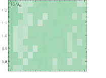
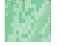
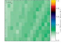
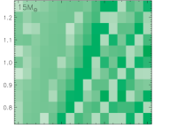
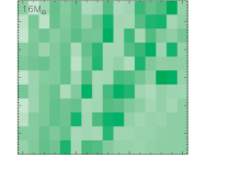
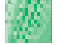
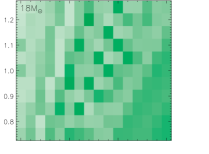
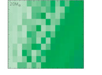
Figure 6: Baryonic mass of the progenitors $\left(M_{\odot}\right)$ for all models as a function of the $R_{3\alpha}$ and $R_{\alpha,12}$ multipliers. The color scale gives the logarithm of the baryonic mass, and the rest of the figure follows the convention of Fig. 3.

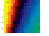
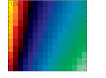
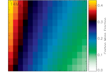
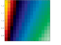
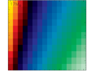
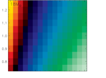
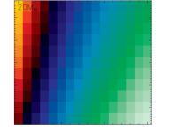
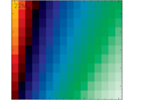
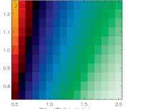
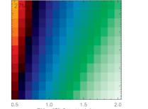
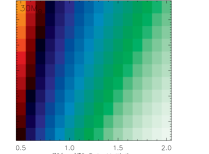
Figure 7: Central carbon mass fractions at the end of core-He burning for all models as a function of the $R_{3\alpha}$ and $R_{\alpha,12}$ multipliers. The color scale gives the carbon mass fraction, and the rest of the figure follows the convention of Fig. 3.

As shown in Fig. 3.4, high $R_{3\alpha}$ and low $R_{\alpha,12}$ multipliers result in higher carbon mass fractions as expected, whereas low $R_{3\alpha}$ and high $R_{\alpha,12}$ multipliers result in lower carbon mass fractions. Comparing Fig. 3.4 and Fig. 3.4 shows an overall inverse relation between the carbon mass fraction and the remnant mass (see also Fig. 6 and Fig. 7).

4 Conclusions

This paper studies the effect of changing the helium burning rates ${}^{\text{12}}$C($\alpha,\gamma$)${}^{\text{16}}$O and ${}^{\text{4}}$He($2\alpha,\gamma$)${}^{\text{12}}$C independently to map the effects on stellar evolution and nucleosynthesis. We follow the entire evolution from hydrogen burning through the SN explosion, including wind and SN yields, and considering fallback, mixing, and which stars make SNe ($\xi_{2.5}<0.25$) or collapse to BHs without SN, and finally integrating the yields over an IMF. In total, we calculated nucleosynthesis for a grid of 176 models for each of 12 stellar masses from $\mathrm{12\,M}_{\text{$\odot$}}$ to $\mathrm{30\,M}_{\text{$\odot$}}$ (2112 models). This is by far the most extensive investigation on the effects of rate variations for the helium burning reactions to date, and the first to use updated solar abundances (Lodders, 2009).

Combining constraints on intermediate-mass and weak s-only isotopes, we find a best fit for rate multipliers $\left(R_{\alpha,12},R_{3\alpha}\right)=\left(1.1,0.75\right)$ to $\left(1.6,1.25\right)$ with an average spread of $\approx\pm 0.2$ in $R_{\alpha,12}$. More generally, we find a relation between $R_{\alpha,12}$ and $R_{3\alpha}$ for good fits to nucleosynthesis given by $R_{\alpha,12}=1.0R_{3\alpha}+(0.35\pm 0.2)$ in the range $R_{3\alpha}$ = 0.75 to 1.25. We also provide the line of best fit using only the intermediate-mass isotope list, given by $R_{\alpha,12}=1.0R_{3\alpha}+(0.25\pm 0.3)$.

In this analysis, all models are assumed to have a final kinetic energy of the ejecta of 1.2 B. Real supernovae have a range of explosion energies. A larger explosion energy would allow successful SNe above the $\xi_{2.5}=0.25$ limit, since now larger densities would be required to overcome this larger energy to prevent a successful SN explosion. It would also cause more material above the Fe core to escape the gravitational potential, resulting in a smaller mass cut and remnant mass for models already below $\xi_{2.5}=0.25$.

Small changes in the reaction rates can result in significant differences in the convection structure of the star, which is not just a numerical artifact but due to the physics of shell burning. This introduces “noise” into the comparisons, and is a warning for calculations done for specific cases; the general conclusion may be influenced by isolated processes. Given an astrophysical model that includes all the important physics with perfectly known physical input parameters, the values for the standard deviations shown in the figures should have a minimum region reflecting only the uncertainties in isotopic abundances. We know, however, that the stellar model used is only approximate and can affect the nucleosynthesis, as discussed in Section 3.3. For the isotopes we compare in this work, however, the assumption that solar composition stars should produce about their solar ratios is reasonable.

If we change the parameters of the models or improve the completeness of the models, we expect the best fit rates to change also. Hence it is not necessarily the case that the best fit rate for an observable (in our case the abundances) coincides with the true rate. This suggests that the best reaction rates we obtain in our analyses are at some level effective rates. Analogous procedures have been used in many areas of physics. For example, in the shell model of nuclear physics, an effective nucleon-nucleon interaction (close to but not identical to the true interaction) is chosen to fit the low-lying spectra of many nuclei, and this reaction is very successfully used to predict other observables. Similarly, we think that the present procedure can provide better predictions of other astrophysical quantities, remnant masses or neutrinos synthesis of certain isotopes, for example.

Whereas our comparisons do not have the power to accurately determine the helium burning reaction rates, they do show that the experimental values are not too far from the truth and that changes needed to compensate (in an effective interaction sense) for model uncertainties are not large. Thus, similar calculations necessary to assess the situation, as overall model uncertainties decrease, will be less demanding; we have shown that a significant part of the uncertainty space is irrelevant. It is also clear that if one of the two helium burning reactions is much better determined, the effective rate for the other will be much better determined. For example, if it is later determined that $R_{3\alpha}$ is near 1.25 times the present experimental centroid value, then the best fit $R_{\alpha,12}$ will be 33 % larger than the experimental centroid value. It may also happen that if both reactions become well determined, they would not agree with the effective interaction that best reproduces the abundances. In such an event, this work may still serve to provide an evaluation of other model uncertainties and point the way to improvements.

Appendix A Appendix

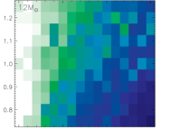
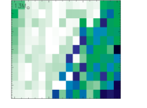
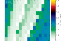
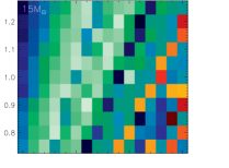
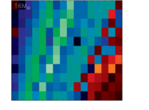
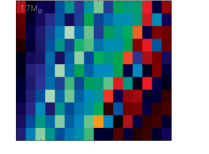
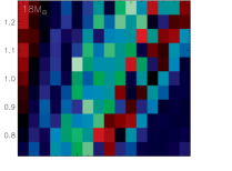
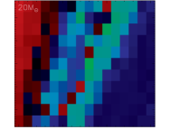
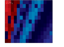
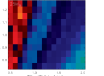
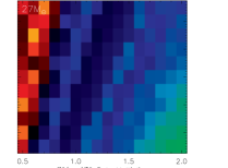
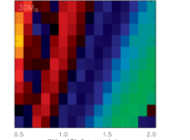
Figure 3: Standard deviations of the production factors of intermediate-mass isotopes for all models as a function of the $R_{3\alpha}$ and $R_{\alpha,12}$ multipliers. The horizontal axis gives the $R_{\alpha,12}$ multiplier, the vertical axis gives the $R_{3\alpha}$ multiplier, and the color scale gives the logarithm of the standard deviations.

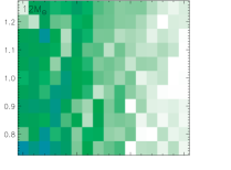
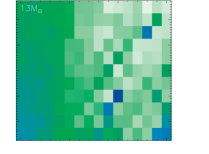
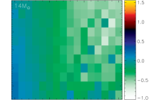
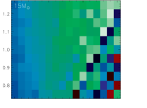
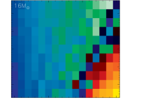
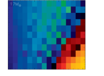
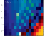
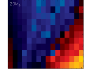
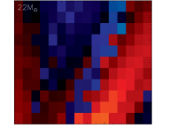
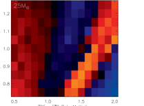
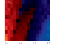
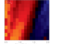
Figure 4: Standard deviations of the production factors of weak s-only isotopes for all models as a function of the $R_{3\alpha}$ and $R_{\alpha,12}$ multipliers. The figure follows the convention of Fig. 3.

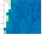
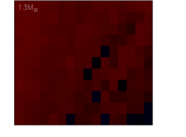
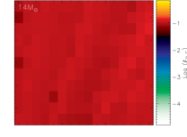
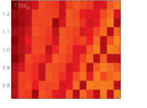
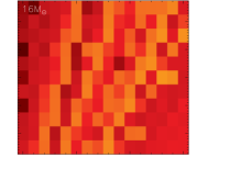
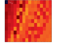
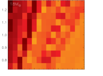
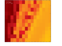
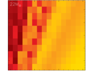
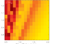
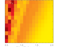
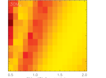
Figure 5: Compactness parameter values for all models as a function of the $R_{3\alpha}$ and $R_{\alpha,12}$ multipliers. The color scale gives the logarithm of the compactness parameter, and the rest of the figure follows the convention of Fig. 3.

References

- Austin et al. (2011) Austin, S., Heger, A., & Tur, C., 2011, Phys. Rev. L, 106, 15
- Buchmann (2000) Buchmann, L., 2000, Priv. Comm.
- Burbidge et al. (1957) Burbidge, M., Burbidge, G., Fowler, W, & Hoyle, F., 1957, Rev. Mod. Phys., 29, 547
- Caughlan and Fowler (1988) Caughlan, G., & Fowler, W., 1988, At. Data & Nucl. Data Tab., 40, 283
- Chernykh et al. (2010) Chernykh, M., Feldmeier, H., Neff, T., von Neumann-Cosel, P., & Richter, A., 2010, Phys. Rev. Lett. 105, 02250
- Chieffi and Limongi (2012) Chieffi, A., & Limongi, M., 2012, arXiv:1212.2759v1
- Diehl et al. (2006) Diehl, R., Prantzos, N., & von Ballmoos, P., 2006, Nucl. Phys. A, 777, 70
- Heger et al. (2001) Heger, A., Woosley, S. E., Mart nez-Pinedo, G., & Langanke, K., 2001, ApJ, 560, 307
- Heger and Woosley (2010) Heger, A., & Woosley, S., 2010, ApJ, 724, 341
- Iliadis et al. (2011) Iliadis, C., Champagne, A., Chieffi, A., & Limongi, M., 2011, ApJ, 193, 16
- Jacobson and Friel (2012) Jacobson, H., & Friel, E., 2012, AAS, 219
- Jiang et al. (2007) Jiang, C., Rehm, K., Back, B., & Janssens, R., 2007, Phys. Rev. C., 75, 1
- Lattimer and Prakash (2001) Lattimer, J. M., & Prakash, M. 2001, ApJ, 550, 426
- Lattimer and Prakash (2010) Lattimer, J., & Prakash, M., 2010, arXiv1012.3208L
- Leising and Diehl (2009) Leising, M., & Diehl, R., 2009, arXiv:0903.0772
- Lodders (2009) Lodders, K., 2009, arXiv:1010.2746v1
- Maiorca et al. (2011) Maiorca, E., Randich, S., Busso, M., Magrini, L., & Palmerini, S., 2011, ApJ, 736, 120
- Maiorca et al. (2012) Maiorca, E., Magrini, L., Busso, M., Randich, S., Palmerini, S., & Trippella, O., 2012, ApJ, 747, 53
- Mashonkina et al. (2007) Mashonkina, L., Vinogradova, A., Ptitsyn, D., Khokhlova, V., & Chernetsova, T., 2007, ARep, 51, 903
- Notani et al. (2012) Notani, M., Esbensen, H., Fang, X., Bucher, B., Davies, P., Jiang, C., et al., 2012, Phys. Rev. C., 85, 014607
- Nguyen et al. (2012) Nguyen, N., Nunes, F., Thompson, I., & Brown, E., 2012, Phys. Rev. Lett. 109, 14
- O’Connor and Ott (2011) O’Connor, & E., Ott, C., 2011, ApJ, 730, 70
- Pignatari et al. (2010) Pignatari, M., Gallino, R., Heil, M., Wiescher, M., Kppeler, F., Herwig, F., et al, 2010, ApJ, 710, 1557
- Pignatari et al. (2013) Pignatari, M., Hirschi, R., Wiescher, M., Gallino, R., Bennett, M., Beard, M., et al., 2013, ApJ, 762, 31
- Raiteri et al. (1993) Raiteri, C., Gallino, R., Busso, M., Neuberger, D., & Kppeler, F., 1993, ApJ, 419, 207
- Rauscher et al. (2002) Rauscher, T., Heger, A., Hoffman, R., & Woosley, S., 2002, ApJ, 576, 323348
- Rayet and Hashimoto (2000) Rayet, M., Hashimoto, M., 2000, A&A, 354, 740
- Spillane et al. (2007) Spillane, T., Raiola, F., Rolfs, C., Schrmann, D., Strieder, F., Zeng, S., et al. 2007, Phys. Rev. Lett., 98, 122501
- Tolos et al. (2012) Tolos, L., Sagert, I., Chatterjee, D., Schaffner-Bielich, J., & Sturm, C., 2012, arXiv1211.0427T
- Tur et al. (2007) Tur, C, Heger, A., & Austin, S., 2007, ApJ, 671, 821
- Tur et al. (2009) Tur, C, Heger, A., & Austin, S., 2009, ApJ, 702, 1068
- Tur et al. (2010) Tur, C, Heger, A., & Austin, S., 2010, ApJ, 718, 357
- Ugliano et al. (2012) Ugliano, M., Janka, H., Marek, A., & Arcones, A., 2012, ApJ, 757, 69
- Weaver et al. (1978) Weaver, T., Zimmerman, G., & Woosley, S., 1978, ApJ, 225, 1021
- West and Heger (2012) West, C., & Heger, A., 2012, arXiv:1203.5969v1
- Woosley and Weaver (1998) Woosley, S., Weaver, T., 1988, Phys. Rep., 163, 79
- Woosley et al. (2002) Woosley, S., Heger, A., & Weaver, T., 2002, Rev. of Mod. Phys., 74 1015
- Woosley et al. (2003) Woosley, S., Heger, A., Rauscher, T., & Hoffman, R., 2003, Nucl. Phys. A, 718, 3c
- Woosley and Heger (2007) Woosley, S., & Heger, A.,2007, Phys. Rep. 442, 269
- Woosley (2012) Woosley, S., 2012, private communication
- Zhang et al. (2008) Zhang, W., Woosley, S., & Heger, A., 2008, ApJ, 679, 639
- Zickefoose (2010, unpublished) , J., 2010, Ph.D. Thesis, University of Connecticut