Third virial coefficient of the unitary Bose gas

Abstract

By unitary Bose gas we mean a system composed of spinless bosons with $s$-wave interaction of infinite scattering length and almost negligible (real or effective) range. Experiments are currently trying to realize it with cold atoms. From the analytic solution of the three-body problem in a harmonic potential, and using methods previously developed for fermions, we determine the third cumulant (or cluster integral) $b_{3}$ and the third virial coefficient $a_{3}$ of this gas, in the spatially homogeneous case, as a function of its temperature and the three-body parameter $R_{t}$ characterizing the Efimov effect. A key point is that, converting series into integrals (by an inverse residue method), and using an unexpected small parameter (the three-boson mass angle $\nu=\pi/6$), one can push the full analytical estimate of $b_{3}$ and $a_{3}$ up to an error that is in practice negligible.

I Introduction

The field of quantum gases has been exploring, in the last decade, the strongly interacting regime, thanks to the possibility of tuning the $s$-wave scattering length $a$ to arbitrarily large values (in absolute value) with the Feshbach resonance technique Heinzen ; Julienne . This opens up the perspective of studying a fascinating object, the unitary gas, such that the interactions among particles have an infinite $s$-wave scattering length and a negligible range. The two-body scattering amplitude then reaches the maximal modulus allowed by unitarity of the $S$ matrix, and the gas is maximally interacting.

For the spin-$1/2$ Fermi gases, the experimental realisation and characterisation of the strongly interacting regime have been fully successful prems ; BookZwerger , recently culminating with the measurement of the equation of state of the unitary gas, both at high and low temperature $T$ Nascimbene ; Navon ; Zwierlein . In the unpolarized case, this has allowed a precise comparison with the theoretical predictions, that are pushed to their limits. At zero temperature, in practice $T/T_{F}\ll 1$ where $T_{F}$ is the Fermi temperature, the measurements have confirmed the precision of the most recent variational fixed-node calculations, as far as the universal number $\xi=\mu/(k_{B}T_{F})$ is concerned, $\mu$ being the chemical potential of the gas Gezerlis . For the superfluid phase transition, the experiments confirm the expected universality class and find a value of the critical temperature $T_{c}$ that slightly corrects the result of the first Quantum Monte Carlo calculations Svistunov and that confirms the one of most recent Quantum Monte Carlo calculations Goulko . Above $T_{c}$, the measurements at MIT are in remarkable agreement with the diagrammatic Monte Carlo method BDMC . Finally, in the non-degenerate regime $T>T_{F}$, the experiments at ENS have been able to confirm the value of the third virial coefficient $a_{3}$ of the spatially homogeneous gas, already theoretically deduced Drummond from the analytical solution of the three-body problem in a harmonic trap Werner and reproduced later on by a diagrammatic method Leyronas ; these experiments are even ahead of theory in getting the value of $a_{4}$, not yet extracted by theory in a reliable way from the four-body problem Blume .

For the strongly interacting gases of spinless bosons, the experimental studies are less advanced, due to the Efimov effect Efimov : The effective three-body attraction predicted by Efimov, and leading to his famous weakly bound trimers, for which there is now an experimental signature Revue , leads to a strong increase of atomic losses in the gas, due to three-body collisions with strongly exothermic formation of deeply bound dimers. In the unitary limit, one can at the moment prepare a stable and thermal equilibrium Bose gas only in the non-degenerate regime $\rho\lambda^{3}\ll 1$ SalomonPetrov , where $\rho$ is the gas density and $\lambda=(2\pi\hbar^{2}/mk_{B}T)^{1/2}$ is the thermal de Broglie wavelength: The two-body elastic collision rate, scaling as $\frac{\hbar}{m}\rho\lambda$, then overcomes the three-body loss rate scaling as $\frac{\hbar}{m}\rho\lambda^{4}$ Esry . Fortunately, there exists a few ideas to explore to reduce losses, such as taking advantage of the loss-induced Zeno effect in an optical lattice Zoller , or simply the use of narrow Feshbach resonances Petrov ; Wang .

On a theoretical point of view, the study of the unitary Bose gas is just starting. Most of the works do not take into account in an exact way the three-or-more-body correlations Pandha ; Stoof ; Ho2012 ; they cannot thus quantitatively account for the fact that resonant interactions among bosons involve the three-body parameter $R_{t}$, a length giving the global energy scale in the Efimov trimer spectrum (no energy scale can be given by the scattering length here, since it is infinite). As a consequence, the various phases under which the unitary Bose system may exist at thermal equilibrium, as functions of temperature, remain to be explored. At zero temperature, inclusion of a hard-core three-body interaction, allowing one to adjust the value of $R_{t}$ and to avoid the system collapse, has allowed one to show, with numerical calculations limited to about ten particles, that the bosons form a $N$-body bound state, with an energy that seems to vary linearly with $N$ vonStecher , which suggests a phase of bounded density at large $N$, for example a liquid. At high temperature (more precisely at low density $\rho\lambda^{3}\to 0$), the natural theoretical approach is the virial expansion Beth , that we recall here for the spatially homogeneous gas Huang :

$$\frac{P\lambda^{3}}{k_{B}T}=\sum_{n\geq 1}a_{n}(\rho\lambda^{3})^{n}$$ (1)

where $P$ is the gas pressure. The coefficient $a_{n}$ is precisely the $n^{\mathrm{th}}$ virial coefficient. In practice, it will be more convenient to determine the coefficients $b_{n}$ of the expansion of the grand potential $\Omega$ in powers of the fugacity $z=e^{\beta\mu}$, with the chemical potential $\mu$ tending to $-\infty$:

$$\Omega=-\frac{V}{\lambda^{3}}k_{B}T\sum_{n\geq 1}b_{n}z^{n},$$ (2)

with $V$ the system volume and $\beta=1/(k_{B}T)$. The coefficients $b_{n}$ are called cluster integrals in reference Huang . Since $-\beta\Omega$ is the logarithm of the grand canonical partition function, it is natural to call $b_{n}$ the $n^{\mathrm{th}}$ cumulant, as we shall do in this paper. The knowledge of all cumulants up to order $n$ included allows one to determine all the virial coefficients up to the same order. Note that $a_{1}=b_{1}=1$ by construction; the higher order expressions that are useful here are deduced in a simple way from the thermodynamic equalities $\Omega=-PV$ and $N=-\partial_{\mu}\Omega$ Huang :

$$a_{2}=-b_{2}\ \ \ \mbox{and}\ \ \ a_{3}=4b_{2}^{2}-2b_{3}.$$ (3)

Contrarily to the fermionic case, the cumulant $b_{3}$ and the virial coefficient $a_{3}$ of the bosons in the unitary limit are not pure numbers, they rather are not yet explicitly determined functions of the three-body parameter. After the pioneering works PaisUlhenbeck1959 , there exist for sure formal expressions of $b_{3}$ in the general quantum case involving Faddeev equations GibsonReiner , the $S$-matrix Ma , Mayer diagrams Royer , an Ursell operator Huang ; Laloe1995 . The most operational form seems to be the one of GibsonReiner written in terms of a three-body scattering amplitude BedaqueRupak2003 , but its evaluation for the unitary Bose gas is, to our knowledge, purely numerical, and for three different values of $R_{t}$ only BedaqueRupak2003 . Here, we show on the contrary that $b_{3}$ can be obtained analytically, from the solution of the harmonically trapped three-boson problem Pethick ; Werner .

In the first stage of the solution, one considers the system at thermal equilibrium in the harmonic potential $U(\mathbf{r})=\frac{1}{2}m\omega^{2}r^{2}$, $\omega$ being the free oscillation angular frequency, and one expresses the third cumulant $B_{3}(\omega)$ of the trapped gas, defined by the expansion (5) to come, in terms of the partition functions of $n$-body problems in the trap, $1\leq n\leq 3$. In theoretical physics, a formal “harmonic regularisator” was already introduced to obtain the second Ouvry and third Cabe ; Law virial coefficients of a gas of anyons. The same technique was then used in the case of cold fermionic atoms Drummond , to take advantage of the fact that the three-body problem is solvable in the unitary limit; note that it is then not a pure calculation trick anymore since the trapping can be realised experimentally.

In the second stage, one takes the limit of a vanishing trap spring constant. As shown by the local density approximation Drummond , which is actually exact in that limit, the cumulants $b_{n}$ of the homogeneous gas are then given by Ouvry ; Drummond

$$\frac{b_{n}}{n^{3/2}}=\lim_{\omega\to 0}B_{3}(\omega)\equiv B_{3}(0^{+}).$$ (4)

In Drummond , this limit is evaluated purely numerically for the fermions. We shall insist here on showing that one can actually go much farther analytically.

II Expression of $\Delta B_{3}$ in terms of canonical partition functions

When the chemical potential $\mu\to-\infty$ at fixed temperature, which corresponds to a low density limit, the grand potential of the trapped unitary Bose gas can be expanded as

$$\Omega=-k_{B}TZ_{1}\sum_{n\geq 1}B_{n}z^{n}$$ (5)

where $Z_{N}$ is the canonical partition function with $N$ particles, $z=\exp(\beta\mu)$ is the fugacity, and $B_{n}(\omega)$ is the $n^{\mathrm{th}}$ cumulant of the trapped gas. By construction, $B_{1}(\omega)\equiv 1$. One also has, by definition, $\Omega=-k_{B}T\ln(1+\sum_{N\geq 1}Z_{N}z^{N}).$ By order-by-order identification in $z$, as for example in Drummond , one finds

$$B_{2}=\frac{Z_{2}}{Z_{1}}-\frac{1}{2}Z_{1}\ \ \ \mbox{and}\ \ \ B_{3}=\frac{Z_{3}}{Z_{1}}-Z_{2}+\frac{1}{3}Z_{1}^{2}.$$ (6)

In reality, one shall calculate the deviation from the ideal gas,

$$\Delta B_{n}=B_{n}-B_{n}^{(0)}$$ (7)

where $B_{n}^{(0)}(\omega)$ is the $n^{\mathrm{th}}$ cumulant of the trapped ideal gas. Similarly one introduces $\Delta Z_{N}=Z_{N}-Z_{N}^{(0)}$, noting that $\Delta Z_{1}=0$. As there is furthermore separability of the center of mass in a harmonic trap, both for the ideal gas and for the unitary gas, and as the spectrum of the center of mass is the same as the one of the one-body problem, one is left with partition functions of the $n$-body relative motion, denoted by “rel”:

$$\Delta B_{2} = \frac{\Delta Z_{2}}{Z_{1}}=\Delta Z_{2}^{\rm rel}$$ (8)

$$\Delta B_{3} = \frac{\Delta Z_{3}}{Z_{1}}-\Delta Z_{2}=\Delta Z_{3}^{\rm rel}-\Delta Z_{2}.$$ (9)

It remains to use the expressions for the relative motion spectrum, known in the unitary limit up to $n=3$ Pethick ; Werner .

II.1 Case $N=2$

The interactions modify the spectrum of the relative motion only in the sector of angular momentum $l=0$, and in the unitary limit, their effect reduces to a downward shift by $\hbar\omega$ of the unperturbed spectrum, $E_{l=0,n}^{(0)}=(2n+3/2)\hbar\omega$ Wilkens , so one finds

$$\Delta Z_{2}^{\rm rel}=(e^{x}-1)\sum_{n\geq 0}e^{-x(2n+3/2)}=\frac{e^{-x/2}}{1+e^{-x}}=\Delta B_{2}$$ (10)

where $x=\beta\hbar\omega$. As a consequence, using equation (8) and $Z_{1}=[e^{-x/2}/(1-e^{-x})]^{3}$:

$$\Delta Z_{2}=\frac{e^{-2x}}{(1-e^{-x})^{2}(1-e^{-2x})}.$$ (11)

Another consequence is that the second cumulant of the spatially homogeneous unitary Bose gas is obtained from the expression $B_{2}^{(0)}(\omega)=\frac{1}{2}(\frac{1}{2\operatorname{ch}(x/2)})^{3}$ (deduced by a direct calculation) by taking the $\omega\to 0$ limit and using (4):

$$\frac{b_{2}}{2^{3/2}}=\frac{1}{2}+\frac{1}{2^{4}}.$$ (12)

II.2 Case $N=3$

As shown in Werner , the problem of three trapped bosons has a particular class of eigenstates, called laughlinian in what follows, with a wavefunction that vanishes when there is at least two particles in the same point. These eigenstates thus have energies that are independent of the scattering length $a$ and they do not contribute to $\Delta Z_{3}$. It therefore remains to sum over the non-laughlinian eigenstates for the non-interacting case ($a=0$) and for the unitary limit ($1/a=0$).

In the case $a=0$, using as in Drummond the Efimov ansatz for the three-body wavefunction one finds that the non-laughlinian eigenenergies of the relative motion are

$$E_{\rm rel}^{(0)}=(u_{l,n}^{(0)}+1+2q)\hbar\omega\ \ \ \mbox{of degeneracy}\ 2l+1,$$ (13)

where $l,n,q$ span the set of natural integers, with $l$ quantifying the angular momentum and $q$ the excitation of the hyperradial mode WernerSym . The $u^{(0)}\geq 0$ are the roots of the function $s\mapsto 1/\Gamma(\frac{l-s}{2}+1)$ :

$$u_{l,n}^{(0)}=l+2+2n.$$ (14)

In reality, one must keep in the spectrum (13) the physical roots only, such that the Efimov ansatz is not identically zero. The two known unphysical roots are $u^{(0)}=4$ for $l=0$, and $u^{(0)}=3$ for $l=1$. But this will not play any role in what follows.

In the case $1/a=0$, using the Efimov ansatz as in Werner , subjected to the Wigner-Bethe-Peierls contact conditions, one gets the transcendental equation $\Lambda_{l}(s)=0$, with GasaneoBirse

$$\Lambda_{l}(s)=\cos\nu-(-\sin\nu)^{l}\frac{\Gamma(\frac{l+1+s}{2})\Gamma(\frac{l+1-s}{2})}{\pi^{1/2}\Gamma(l+\frac{3}{2})}\\ \times{}_{2}F_{1}\left(\frac{l+1+s}{2},\frac{l+1-s}{2},l+\frac{3}{2};\sin^{2}\nu\right)$$ (15)

where ${}_{2}F_{1}$ is the Gauss hypergeometric function and the usual mass angle what introduced, which is given for three bosons by

$$\nu=\arcsin\frac{1}{2}=\frac{\pi}{6}.$$ (16)

In practice, we shall also use the representation derived in Tignone for fermions and easily transposed to the bosonic case, in terms of Legendre polynomials $P_{l}(X)$ :

$$\!\!\!\Lambda_{l}(s)\!\! \!\stackrel{{\scriptstyle l\,{\rm even}}}{{=}}\! \!\!\cos\nu-\frac{2}{\sin\nu}\!\!\int_{0}^{\nu}\!\!d\theta P_{l}\left(\frac{\sin\theta}{\sin\nu}\right)\frac{\cos(s\theta)}{\cos(s\pi/2)}$$ (17)

$$\!\!\!\Lambda_{l}(s)\!\! \!\stackrel{{\scriptstyle l\,{\rm odd}}}{{=}}\! \!\!\cos\nu+\frac{2}{\sin\nu}\!\!\int_{0}^{\nu}\!\!d\theta P_{l}\left(\frac{\sin\theta}{\sin\nu}\right)\frac{\sin(s\theta)}{\sin(s\pi/2)},$$ (18)

which allows us to explicitly write $\Lambda_{l}(s)$ with the sine function and rational fractions of $s$.

II.3 Efimovian channel

In the zero-angular-momentum sector, $l=0$, $\Lambda_{l}(s)$ has one and only one root $u_{0,0}\in i\mathbb{R}^{+}$ Werner , usually noted as

$$u_{0,0}=s_{0}=i|s_{0}|,\ \ |s_{0}|=1,006\,237\,825\,\ldots$$ (19)

This root gives rise to the efimovian channel, where the eigenenergies $\epsilon_{q}(\omega)$ of the relative motion solve a transcendental equation Pethick ; Werner that one can rewrite as in Werner_gen2 to make explicit and univocal the dependence with the quantum number $q\in\mathbb{N}$ :

$$\operatorname{Im}\ln\Gamma\Big{(}\frac{1+s_{0}-\epsilon_{q}/(\hbar\omega)}{2}\Big{)}+\frac{|s_{0}|}{2}\ln\Big{(}\frac{2\hbar\omega}{E_{t}}\Big{)}+q\pi=0,$$ (20)

the function $\ln\Gamma(z)$ being taken with its standard determination (branch cut in $\mathbb{R}^{-}$). In the limit $\omega\to 0$ for a fixed $q$, this reproduces the geometric sequence of Efimov trimers:

$$\epsilon_{q}(\omega)\to\epsilon_{q}(0^{+})=-e^{-2\pi q/|s_{0}|}E_{t},$$ (21)

which shows that $E_{t}=2\exp[\frac{2}{|s_{0}|}\operatorname{Im}\ln\Gamma(1+s_{0})]\hbar^{2}/(mR_{t}^{2})$, $R_{t}$ being the three-body parameter according to the convention of Werner . In a strict zero-range limit, $q$ would span $\mathbb{Z}$ and the spectrum would be unbounded below, which would prevent thermal equilibrium of the system. As noted by Efimov Efimov , however, in any given interaction model of finite range $b$, including experimental reality, the geometric form (21) of the spectrum only applies to the trimers of binding energy much smaller than $\hbar^{2}/(mb^{2})$, possible more deeply bound trimers being out of the unitary limit and non universal. Here, the quantum number $q=0$ thus simply corresponds to the first state having (almost) reached the unitary limit. For an interaction to allow for the realisation of the unitary Bose gas at thermal equilibrium, $q=0$ must correspond to the true ground trimer, and this is indeed the case for the model of vonStecher and for the narrow Feshbach resonance Petrov_bosons ; Gogolin ; Pricoupenko2010 ; Zwerger : in both situations, $E_{t}$ is indeed of the order of $e^{-2\pi/|s_{0}|}\hbar^{2}/(mb^{2})\ll\hbar^{2}/(mb^{2})$ and the trimer spectrum can be considered as being entirely efimovian, as it is assumed in the present work.

II.4 Universal channels

The real positive roots $(u_{0,n})_{n\geq 1}$ of $\Lambda_{0}(s)$, and the roots $(u_{l,n})_{n\geq 0}$ of $\Lambda_{l}(s)$ for $l>0$, which are all real Werner and taken in what follows to be positive, give rise to universal, that is non-efimovian, states, with eigenenergies of the relative motion that are independent of $R_{t}$:

$$E_{\rm rel}=(u_{l,n}+1+2q)\hbar\omega\ \ \ \mbox{of degeneracy}\ 2l+1,$$ (22)

where $(l,n)$ spans $\mathbb{N}^{2*}$, and $q$ spans $\mathbb{N}$, and the star indicates that the vanishing element [here $(0,0)$] has to be excluded. One can note the similitude with the non-interacting case (13), the quantum number $q$ having the same physical origin Werner . As in the non-interacting case, one must eliminate from the spectrum (22) the unphysical roots $u$, that give a vanishing Efimov ansatz. These unphysical roots, however, are exactly the same ones in both cases , which allows us formally to include them in the partition functions $Z_{3}$ et $Z_{3}^{(0)}$, since their (unphysical) contributions exactly compensate in $\Delta Z_{3}$. Collecting the contributions of the systems with and without interaction of common quantum numbers, we finally obtain:

$$\Delta Z_{3}^{\rm rel}=\sum_{q\geq 0}\left[e^{-\beta\epsilon_{q}(\omega)}-e^{-x(u_{0,0}^{(0)}+1+2q)}\right]\\ \!\!\!\!+\sum_{(l,n)\in\mathbb{N}^{2*}}\sum_{q\geq 0}(2l+1)\left[e^{-x(u_{l,n}+1+2q)}-e^{-x(u_{l,n}^{(0)}+1+2q)}\right].$$ (23)

II.5 Some useful transforms

In order to treat one by one the problems that arise in taking the limit $\omega\to 0$, it is useful to split (23) as the sum of a purely efimovian contribution $S(\omega)$ and of a purely universal contribution $\sigma(\omega)$, up to additive remainders $R(\omega)$ and $\rho(\omega)$. In what follows we shall study the efimovian series

$$S(\omega)\equiv\sum_{q\geq 0}\left[e^{-\beta\epsilon_{q}(\omega)}-e^{-2qx}\right],$$ (24)

that reproduces the first sum in (23) up to the remainder

$$R(\omega)=\sum_{q\geq 0}\Big{[}e^{-2qx}-e^{-x(u_{0,0}^{(0)}+1+2q)}\Big{]}=\frac{1-e^{-3x}}{1-e^{-2x}}.$$ (25)

We shall see that it is a doubly clever idea to introduce the universal series

$$\sigma(\omega)=\!\!\!\sum_{(l,n)\in\mathbb{N}^{2*}}\sum_{q\geq 0}(2l+1)\Big{[}e^{-x(u_{l,n}+1+2q)}-e^{-x(v_{l,n}+1+2q)}\Big{]},$$ (26)

with

$$v_{l,n}=l+1+2n.$$ (27)

First, this provides a numerical advantage Drummond , since $v_{l,n}$ is the large-$l$-or-$n$ equivalent of $u_{l,n}$ introduced in equation (17) of reference Werner , so that the series $\sigma$ rapidly converges. Second, as it is apparent in the form (15), the $(v_{l,n})_{n\geq 0}$ are the positive poles of the function $\Lambda_{l}(s)$; the writing (26) is thus reminiscent of the residue theorem, and we shall soon take advantage of this fact. As $v_{l,n}=u_{l,n}^{(0)}-1$, $\sigma$ reproduces the second sum of (23) up to the remainder

$$\rho(\omega)=\!\!\!\sum_{(l,n)\in\mathbb{N}^{2*}}\sum_{q\geq 0}(2l+1)\Big{[}e^{-x(v_{l,n}+1+2q)}-e^{-x({u}_{l,n}^{(0)}+1+2q)}\Big{]}.$$ (28)

With the generating function method, one gets $\sum_{l\geq 0}(2l+1)e^{-lx}=(1-2\frac{d}{dx})\frac{1}{1-e^{-x}}=(1+e^{-x})/(1-e^{-x})^{2}$. This, together with the identities (11) and (25), leads to $\rho(\omega)=\Delta Z_{2}+1-R(\omega)$, and (9) reduces to the simple writing

$$\Delta B_{3}(\omega)=S(\omega)+\sigma(\omega)+1.$$ (29)

This equation (29) is the bosonic equivalent of the fermionic expressions (56,58) of reference Drummond , from which it differs mainly through the contribution $S(\omega)$ of the efimovian channel.

III Analytical transforms and $\omega\to 0$ limit

The most relevant physical quantity being the third cumulant of the spatially homogeneous gas, we must now, according to (4), take the limit of a vanishing trap spring constant. An explicit calculation for the trapped ideal gas gives

$$B_{3}^{(0)}(\omega)=\frac{1}{3}\left(\frac{e^{-x}(1-e^{-x})}{1-e^{-3x}}\right)^{3}\underset{\omega\to 0}{\to}\frac{1}{3^{4}}.$$ (30)

In the unitary case, the method of reference Werner_gen2 allows one to determine $S(0^{+})$ exactly; furthermore, as we shall see, the sum over $n$ in equation (26) and the $x\to 0$ limit can be performed analytically, and the resulting integrals in $\sigma(0^{+})$, that are very simple to evaluate numerically, can also be usefully evaluated by taking the mass angle $\nu$ as a small parameter.

III.1 Working on the efimovian contribution $S(\omega)$

For an arbitrary positive number $A$, with $A\gg 1$, we split as in Werner_gen2 the series (26) into three pieces, $S=S_{1}+S_{2}+S_{3}$.

In the first (quasi-bound) piece, that contains the states such that $\epsilon_{q}(\omega)<-A\hbar\omega$, the three bosons occupy a spatial zone much smaller than the ground-state harmonic oscillator length $[\hbar/(m\omega)]^{1/2}$, so that the spectrum is close to the free-space spectrum (21):

$$\epsilon_{q}(\omega)=\epsilon_{q}(0^{+})\Big{[}1-\frac{1+|s_{0}|^{2}}{6}\Big{(}\frac{\hbar\omega}{\epsilon_{q}(0^{+})}\Big{)}^{2}+\ldots\Big{]}$$ (31)

As $\epsilon_{q}(0^{+})$ is a geometric sequence, approximating $\epsilon_{q}(\omega)$ with $\epsilon_{q}(0^{+})$ in $S_{1}$ induces an error of the order of the error on the last term, that vanishes as $x/A$. From the same geometric property, the maximal index $q_{1}$ in that first piece diverges only logarithmically, as $\frac{|s_{0}|}{2\pi}\ln[E_{t}/(2\hbar\omega)]$, which allows one to replace each term $e^{-2qx}$ by 1, the resulting error on $S_{1}$ vanishing as $xq_{1}^{2}$. One thus has

$$S_{1}=\sum_{q=0}^{q_{1}}\Big{[}e^{-\beta\epsilon_{q}(0^{+})}-1\Big{]}+o(1).$$ (32)

The second piece contains the intermediate states, such that $|\epsilon_{q}(\omega)|<A\hbar\omega$. As the level spacing between the $\epsilon_{q}(\omega)$ is of order $\hbar\omega$ at least, it contains a finite number $O(A)$ of terms, and each terms vanishes when $\omega$ vanishes, so that $S_{2}=o(1)$.

The third piece contains the states $A<\epsilon_{q}(\omega)$, that reconstruct the free space efimovian scattering states when $\omega\to 0$. On can use for these states the large-$q$ expansion

$$\frac{\epsilon_{q}(\omega)}{\hbar\omega}=2q+\Delta\big{(}\epsilon_{q}(\omega)\big{)}+O(1/q)$$ (33)

where the dimensionless function of the energy $\Delta(\epsilon)$ is given by equation (C6) of Werner_gen2 . In each term of $S_{3}$, one uses the approximation $e^{-2qx}\simeq e^{-\beta\epsilon_{q}}[1+x\Delta(\epsilon_{q})]$, and one replaces the sum over $q$ by an integral over energy; since the level spacings are almost constant, $\epsilon_{q+1}-\epsilon_{q}=2\hbar\omega[1+O(\hbar\omega/\epsilon_{q})]$ WernerThese , one gets

$$S_{3}=-\frac{1}{2}\int_{A\hbar\omega}^{+\infty}d\epsilon\,e^{-\beta\epsilon}\beta\Delta(\epsilon)+o(1).$$ (34)

Collecting the three pieces and writing up $\Delta(\epsilon)$ explicitly as in Werner_gen2 , one finally obtains for $\omega\to 0$:

$$S(0^{+})=\Big{\{}\sum_{q\geq 0}\left[e^{-\beta\epsilon_{q}(0^{+})}-1\right]\Big{\}}+\frac{|s_{0}|}{\pi}\Big{\{}\frac{1}{2}\ln(e^{\gamma}\beta E_{t})\\ -\sum_{p\geq 1}\!e^{-p\pi|s_{0}|}\operatorname{Re}\!\Big{[}\Gamma(-ip|s_{0}|)(\beta E_{t})^{ip|s_{0}|}\Big{]}\!\Big{\}},$$ (35)

where $\gamma=0.577\,215\ldots$ is Euler’s constant, and the free space trimer energy $\epsilon_{q}(0^{+})$ is given by (21). One can note that the bound state contribution $\sum_{q\geq 0}e^{-\beta\epsilon_{q}(0^{+})}$ is divergent, and has thus to be collected with the contribution of the continuum to obtain the counter-term $-1$ ensuring the convergence of the sum in (35); in the case of the second virial coefficient of a plasma, the (two-body) bound states have an hydrogenoid spectrum, which requires the more elaborated counter-term $-(1+\beta\epsilon_{q})$ to get a converging sum Larkin .

III.2 Working on the universal contribution $\sigma(\omega)$

Let us extract from the definition (26) of $\sigma(\omega)$ the contribution of the angular momentum $l$ and let us sum over $q$, to obtain

$$\sigma=\sum_{l\geq 0}\sigma_{l},\ \ \mbox{with}\ \ \sigma_{l}=\frac{l+\frac{1}{2}}{\operatorname{sh}x}\sum_{n\geq\delta_{l,0}}\Big{(}e^{-xu_{l,n}}-e^{-xv_{l,n}}\Big{)}.$$ (36)

The key point is now that the function $\Lambda_{l}(s)$ has a simple root in $u_{l,n}$ and a simple pole in $v_{l,n}$, so that its logarithmic derivative has a pole in both points, with a residue respectively equal to $+1$ et $-1$. By inverse application of the residue formula, one thus finds for $l>0$ that

$$\sigma_{l}(\omega)\stackrel{{\scriptstyle l>0}}{{=}}\frac{l+\frac{1}{2}}{\operatorname{sh}x}\int_{C}\frac{dz}{2i\pi}\frac{\Lambda_{l}^{\prime}(z)}{\Lambda_{l}(z)}e^{-xz}$$ (37)

where the integral is taken over the contour $C$ that comes from $z=+\infty+i\eta$ ($\eta>0$), moves parallelly to and above the real axis, crosses the real axis close to the origin and then tends to $z=+\infty-i\eta$ moving parallelly to and below the real axis. This contour indeed encloses all the positive roots $(u_{l,n})_{n\geq 0}$ and all the positive poles $(v_{l,n})_{n\geq 0}$ of the function $\Lambda_{l}(z)$. As $\Lambda_{l}(z)$ ($l>0$) has no other roots or poles in the half-plane $\operatorname{Re}{z}\geq 0$, one can unfold $C$ around the origin and map it to the purely imaginary axis $z=iS$:

$$\sigma_{l}(\omega)\stackrel{{\scriptstyle l>0}}{{=}}\frac{l+\frac{1}{2}}{\pi\operatorname{sh}x}\int_{0}^{+\infty}dS\frac{\Lambda_{l}^{\prime}(iS)}{\Lambda_{l}(iS)}i\sin(xS)$$ (38)

where the fact that $\Lambda_{l}^{\prime}(iS)/\Lambda_{l}(iS)$ is an odd function allows one to omit the $\cos(xS)$ and to restrict integration to $S>0$. It is then elementary to take the $x\to 0$ limit, and a simple integration by parts leads to the nice result:

$$\sigma_{l}(0^{+})\stackrel{{\scriptstyle l>0}}{{=}}-\frac{2l+1}{2\pi}\int_{0}^{+\infty}dS\ln\Big{(}\frac{\Lambda_{l}(iS)}{\cos\nu}\Big{)}.$$ (39)

According to (17,18), the function $\Lambda_{l}(iS)/\cos\nu$ exponentially tends to 1 at infinity, so that the integral in (39) rapidly converges.

The case $l=0$ requires some twist of the previous reasoning. First, the pole $v_{0,0}$ of the function $\Lambda_{0}(s)$ does not contribute to $\sigma(\omega)$, since $(l,n)=(0,0)$ is in the efimovian channel. Second, the existence of the efimovian roots $\pm i|s_{0}|$ of $\Lambda_{0}(s)$ prevents one from folding back the integration contour $C$ on the purely imaginary axis. Both points are solved by considering the function $\frac{s^{2}-v_{0,0}^{2}}{s^{2}-s_{0}^{2}}\Lambda_{0}(s)$ rather than the function $\Lambda_{0}(s)$ itself: The rational prefactor suppresses the poles $\pm v_{0,0}$ and the roots $\pm s_{0}$ without destroying the parity invariance that we have used. In the limit $\omega\to 0$, this leads to

$$\sigma_{0}(0^{+})=-\frac{1}{2\pi}\int_{0}^{+\infty}dS\ln\Big{(}\frac{S^{2}+1}{S^{2}-|s_{0}|^{2}}\,\frac{\Lambda_{0}(iS)}{\cos\nu}\Big{)}.$$ (40)

From the writing (17,18) of the functions $\Lambda_{l}(s=iS)$, and using the numerical tools of formal integration software, one obtains in a few minutes, the value of the constant term in $\Delta B_{3}(0^{+})$:

$$1+\sigma(0^{+})=1-0,364\,037\,\ldots=0,635\,962\,\ldots$$ (41)

One observes that $(\sigma_{l}(0^{+}))_{l\geq 1}$ is an alternating sequence with a rapidly decreasing modulus, so that the error due to a truncation in $l$ is bounded by the first neglected term. Analytically, one can obtain the elegant asymptotic form

$$\sigma_{l}(0^{+})\underset{l\to\infty}{\sim}\Big{(}\frac{l}{\pi}\Big{)}^{1/2}\frac{(-\tan\frac{\nu}{2})^{l}}{\cos\frac{\nu}{2}(\cos\nu)^{3/2}},$$ (42)

where $\nu$ is the mass angle (16).

III.3 An entirely analytical evaluation

The fact that $\sigma_{l}(0^{+})$ is rapidly decreasing with the angular momentum, even in the absence of physical interpretation, can be understood from the fact that, for $l>0$, the deviations of $\Lambda_{l}(iS)/\cos\nu$ from unity vanish as $-(-\nu)^{l}$, this is obvious on the writing (15):

$$\delta_{l}(S)\equiv\frac{\Lambda_{l}(iS)}{\cos\nu}-1\underset{\nu\to 0}{=}O(\nu^{l}).$$ (43)

For $\nu=\pi/6$, one finds that, already for $l=1$, the maximum of $|\delta_{l}(S)|$, reached in $S=0$, has the small value $\simeq 0,273$. This gives the idea of treating each $\delta_{l}$ (for $l>0$) as an infinitesimal quantity of order $l$. The series expansion of $\ln[1+\delta_{l}(S)]$ in powers of $\delta_{l}$ in (39) is convergent and generates a convergent expansion of $\sigma_{l}(0^{+})$ :

$$\sigma_{l}(0^{+})\stackrel{{\scriptstyle l>0}}{{=}}\sum_{n\geq 1}\sigma_{l}^{(n)},\ \mbox{with}\ \sigma_{l}^{(n)}=(2l+1)\frac{(-1)^{n}}{n}\int_{\mathbb{R}}\frac{dS}{4\pi}[\delta_{l}(S)]^{n}.$$ (44)

The resulting integral can in principle be calculated analytically by the residue formula, for $0<\nu<\pi/2$, which leads to series that can be expressed in terms of the Bose functions $g_{\alpha}(z)=\sum_{k\geq 1}z^{k}/k^{\alpha}$, also called polylogarithms, but this rapidly becomes tedious at large $l$ or $n$. We thus restrict ourselves to the order 3 included. For $n\leq 2$, it is actually simpler to directly calculate the sum over all $l\geq 1$ of $\sigma_{l}^{(n)}$, that we note as $\sigma_{1:\infty}^{(n)}$. We finally keep as the desired approximation:

$$\sigma(0^{+})\approx\sigma_{0}(0^{+})+\sigma_{1:\infty}^{(1)}+\sigma_{1:\infty}^{(2)}+\sigma_{1}^{(3)}.$$ (45)

The second and third terms of the approximation (45) can be expressed simply for an arbitrary $\nu$ as

$$\!\!\!\!\!\sigma_{1:\infty}^{(1)} \!\!\!=\!\!\! \frac{1}{\pi\cos\nu\,(1+\sin\nu)}-\frac{\operatorname{argth}(\sin\nu)}{\pi\cos\nu\sin\nu}$$ (46)

$$\!\!\!\!\!\sigma_{1:\infty}^{(2)} \!\!\!=\!\!\! \frac{2\nu}{\pi^{2}\sin\nu\cos^{3}\nu}-\frac{4[\frac{7}{8}\zeta(3)-\operatorname{Re}C_{3}-\nu\operatorname{Im}C_{2}]}{(\pi\sin\nu\cos\nu)^{2}}$$ (47)

with $\zeta$ the Riemann function and $C_{\alpha}=g_{\alpha}(e^{2i\nu})-\frac{1}{2^{\alpha}}g_{\alpha}(e^{4i\nu})$. For $\nu=\pi/6$, one has simply $\operatorname{Re}C_{3}=\frac{7}{18}\zeta(3)$ and $\operatorname{Im}C_{2}=\frac{\sqrt{3}}{72}[\psi^{\prime}(\frac{1}{6})-\psi^{\prime}(\frac{5}{6})]$, where $\psi$ is the digamma function and $\psi^{\prime}$ its first order derivative. To be concise, we give the value of the last term of (45) for $\nu=\pi/6$ only:

$$\sigma_{1}^{(3)}=\frac{64}{\pi^{3}\sqrt{3}}\left(\frac{17D_{3}}{432}-\frac{14\zeta(3)}{3}-\frac{403\zeta(5)}{27}+2\right)\\ +\frac{16}{9\pi^{2}}\left(\frac{17D_{3}}{54}+5D_{1}-\frac{322\zeta(3)}{3}-36\right)\\ +\frac{32}{3\pi\sqrt{3}}\left(\frac{5D_{1}}{9}-\frac{112\zeta(3)}{27}+\frac{8}{3}-2\ln 3\right),$$ (48)

with $D_{k}=\psi^{(k)}(\frac{1}{3})-\psi^{(k)}(\frac{2}{3})$, $\psi^{(k)}$ being the $k^{\mathrm{th}}$ derivative of the digamma function, see relation 8.363(8) of reference Gradstein .

It remains to analytically evaluate the first term of (45), that is the universal contribution at zero angular momentum $\sigma_{0}(0^{+})$ given by (40). Since a series expansion of the logarithm around $1$ is not suited to this case, we directly expand to second order in powers of the mass angle: according to (17),

$$\frac{\Lambda_{0}(iS)}{\cos\nu}=1-\frac{2}{\operatorname{ch}(S\pi/2)}-\frac{4}{3}\nu^{2}\frac{1+S^{2}/4}{\operatorname{ch}(S\pi/2)}+O(\nu^{4}).$$ (49)

This first allows one to evaluate the efimovian root

$$|s_{0}|=\theta+\frac{8\nu^{2}}{3\pi\sqrt{3}}(1+\theta^{2}/4)+O(\nu^{4})$$ (50)

where $\theta=\frac{2}{\pi}\operatorname{argch}2=0,838\,401\ldots$, in a way that reproduces (for $\nu=\pi/6$) its exact value (19) within one part per thousand. Then, after a few applications of the residue formula, one obtains the desired approximation up to order 3 included:

$$\sigma_{0}(0^{+})\simeq-\frac{1+\theta^{2}}{8}-\frac{2\nu^{2}}{9\pi\sqrt{3}}\,\theta(1+\theta^{2}/4).$$ (51)

For $\nu=\pi/6$, our analytical approximation (45) then leads to

$$1+\sigma(0^{+})\simeq 1-0,364\,613\,\ldots=0,635\,386\,\ldots$$ (52)

which reproduces the exact value (41) within one part per thousand. Such a precision is sufficient in practice, considering the present uncertainty on the measurements of the equation of state of the ultracold atomic gases Nascimbene ; Navon ; Zwierlein and the fact that $b_{3}$ is the coefficient of a term that has to be small in a weak density expansion.

IV Conclusion

We have shown that one can entirely analytically determine the third cumulant $b_{3}$ of the spatially homogeneous unitary Bose gas of three-body parameter $R_{t}$ and thermal de Broglie wavelength $\lambda$: The result

$$b_{3}=3\sqrt{3}[S(0^{+})+C]\ \ \mbox{with}\ \ C=0,648\ldots$$ (53)

is the sum of a function $S(0^{+})$ of $\lambda/R_{t}$ exactly given by equation (35), and of a constant $C$; we have found an original integral representation of $C$ that makes its numerical evaluation straightforward, and that allows one to perform a perturbative expansion of $C$, in principle to arbitrary order but restricted here to third order included, taking the mass angle $\nu=\pi/6$ as a small parameter. This gives access to the third virial coefficient $a_{3}$ of the unitary Bose gas, combining relations (3) and (12).

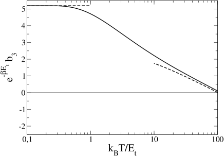
Figure 1: Third cumulant $b_{3}$ of the spatially homogeneous unitary Bose gas: $b_{3}$ is multiplied by $e^{-\beta E_{t}}$ and plotted as a function of temperature $T$ as a solid line. The dashed lined to the left and to the right respectively correspond to the approximations (54) and (55), that have been multiplied by $e^{-\beta E_{t}}$. $(-E_{t})$ is the energy of the ground state (efimovian) trimer, and $\beta=1/(k_{B}T)$.

As shown by the figure, our result has the physical interest of describing the crossover between two limiting regimes, the low-temperature regime $k_{B}T\ll E_{t}$, where $b_{3}$ is dominated by the contribution of the ground state trimer of energy $-E_{t}$:

$$b_{3}\simeq 3\sqrt{3}\,e^{\beta E_{t}},$$ (54)

with $E_{t}\propto\hbar^{2}/(mR_{t}^{2})$, and the regime $k_{B}T\gg E_{t}$, where the trimers are almost fully dissociated:

$$b_{3}\simeq 3\sqrt{3}\frac{|s_{0}|}{2\pi}\ln(e^{\gamma+2\pi C/|s_{0}|}\beta E_{t}).$$ (55)

The exponential approximation (54) agrees with the expression (193) of reference PaisUlhenbeck1959 , that was very simply deduced from the chemical equilibrium condition of the gas. The logarithmic approximation (55) can also be recovered, within a constant factor inside the logarithm, by a calculation that totally differs from ours, the extraction of the loss rate constant $L_{3}$ from the free-space inelastic scattering problem of three bosons SalomonPetrov , further combined with equation (25) of Werner_gen2 that relates (through general arguments) ${\partial b_{3}}/{\partial(\ln R_{t})}$ to $L_{3}$ in the weak inelasticity limit of that scattering problem.

In practice, in the temperature range where the logarithmic approximation (55) well reproduces our values of $b_{3}$, it may be difficult to ensure that the unitary limit is reached, i.e.  that the finite (real or effective) range of the interaction is indeed negligible. In particular, it is not guaranteed that the change of sign of $b_{3}$ at high temperature, as predicted by the zero-range efimovian theory used in this paper, may really be observed for a more realistic model such as the ones of references vonStecher ; Petrov_bosons ; Gogolin ; Pricoupenko2010 , or in ultracold-atom experiments. Answering this question requires the study of a specific model for the interaction and must be kept for future investigation.

References

- (1) J.M. Vogels et al., Phys. Rev. A 56, R1067 (1997).
- (2) C. Chin, R. Grimm, P. Julienne, E. Tiesinga, Rev. Mod. Phys. 82, 1225 (2010).
- (3) K.M. O’Hara et al., Science 298, 2179 (2002); T. Bourdel et al., Phys. Rev. Lett. 91, 020402 (2003);
- (4) The BCS-BEC Crossover and the Unitary Fermi Gas, LNIP 836, edited by W. Zwerger (Springer, Berlin, 2012).
- (5) S. Nascimbène et al., Nature 463, 1057 (2010).
- (6) N. Navon, S. Nascimbène, F. Chevy, C. Salomon, Science 328, 729 (2010).
- (7) Mark J.H. Ku, A.T. Sommer, L.W. Cheuk, M.W. Zwierlein, Science 335, 563 (2012).
- (8) M. M. Forbes, S. Gandolfi, A. Gezerlis, Phys. Rev. Lett. 106, 235303 (2011).
- (9) E. Burovski, N. Prokof’ev, B. Svistunov, M. Troyer, Phys. Rev. Lett. 96, 160402 (2006).
- (10) O. Goulko, M. Wingate, Phys. Rev. A 82, 053621 (2010).
- (11) K. Van Houcke et al., Nature Phys. 8, 366 (2012).
- (12) S. Jonsell, H. Heiselberg, C.J. Pethick, Phys. Rev. Lett. 89, 250401 (2002).
- (13) Xia-Ji Liu, Hui Hu, P. D. Drummond, Phys. Rev. Lett. 102, 160401 (2009); Phys. Rev. A 82, 023619 (2010).
- (14) F. Werner, Y. Castin, Phys. Rev. Lett. 97, 150401 (2006).
- (15) X. Leyronas, Phys. Rev. A 84, 053633 (2011).
- (16) D. Rakshit, K. M. Daily, D. Blume, Phys. Rev. A 85, 033634 (2012).
- (17) V. Efimov, Sov. J. Nucl. Phys. 12, 589 (1971).
- (18) F. Ferlaino, A. Zenesini, M. Berninger, B. Huang, H.-C. Nägerl, R. Grim, Few-Body Syst. 51, 113 (2011).
- (19) B. S. Rem et al., http://hal.archives-ouvertes.fr/hal-00768038
- (20) J. P. D’Incao, H. Suno, B. D. Esry, Phys. Rev. Lett. 93, 123201 (2004).
- (21) F. Werner, Y. Castin, Phys. Rev. A 86, 053633 (2012).
- (22) A. J. Daley et al., Phys. Rev. Lett. 102, 040402 (2009).
- (23) J. Levinsen, T.G. Tiecke, J.T.M. Walraven, D.S. Petrov, Phys. Rev. Lett. 103, 153202 (2009).
- (24) Yujun Wang, J. P. D’Incao, B.D. Esry, Phys. Rev. A 83, 042710 (2011).
- (25) S. Cowell et al., Phys. Rev. Lett. 88, 210403 (2002).
- (26) J. M. Diederix, T. C. F. van Heijst, H. T. C. Stoof, Phys. Rev. A 84, 033618 (2011).
- (27) Weiran Li, Tin-Lun Ho, Phys. Rev. Lett. 108, 195301 (2012).
- (28) J. von Stecher, J. Phys. B 43, 101002 (2010).
- (29) E. Beth, G.E. Uhlenbeck, Physica III 8, 729 (1936); Physica IV 10, 915 (1937).
- (30) K. Huang, in Statistical Mechanics, p. 427 (Wiley, New York, 1963).
- (31) A. Pais, G.E. Uhlenbeck, Phys. Rev. 116, 250 (1959).
- (32) W.G. Gibson, Phys. Letters 21, 619 (1966); A.S. Reiner, Phys. Rev. 151, 170 (1966).
- (33) R. Dashen, Shang-keng Ma, H.J. Bernstein, Phys. Rev. 187, 345 (1969); S. Servadio, Il Nuovo Cimento 102, 1 (1988).
- (34) A. Royer, J. Math. Phys. 24, 897 (1983).
- (35) P. Grüter, F. Laloë, J. Physique I 5, 181 (1995).
- (36) P.F. Bedaque, G. Rupak, Phys. Rev. B 67, 174513 (2003).
- (37) A. Comtet, Y. Georgelin, S. Ouvry, J. Phys. A 22, 3917 (1989).
- (38) J. McCabe, S. Ouvry, Phys. Lett. B 260, 113 (1990).
- (39) J. Law, Akira Suzuki, R.K. Bhaduri, Phys. Rev. A 46, 4693 (1992).
- (40) T. Busch, B.G. Englert, K. Rzazewski, M. Wilkens, Found. Phys. 28, 549 (1998).
- (41) F. Werner, Y. Castin, Phys. Rev. A 74, 053604 (2006).
- (42) G. Gasaneo, J.H. Macek, J. Phys. B 35, 2239 (2002); M. Birse, J. Phys. A 39, L49 (2006).
- (43) Y. Castin, E. Tignone, Phys. Rev. A 84, 062704 (2011).
- (44) D.S. Petrov, Phys. Rev. Lett. 93, 143201 (2004).
- (45) A.O. Gogolin, C. Mora, R. Egger, Phys. Rev. Lett. 100, 140404 (2008).
- (46) L. Pricoupenko, Phys. Rev. A 82, 043633 (2010).
- (47) R. Schmidt, S.P. Rath, W. Zwerger, Eur. Phys. J. B 85, 386 (2012).
- (48) F. Werner, PhD thesis, University Paris 6 (2008), http://tel.archives-ouvertes.fr/tel-00285587
- (49) A.I. Larkin, Sov. Phys. JETP 11, 1363 (1960).
- (50) I.S. Gradshteyn, I. M. Ryzhik, in Tables of Integrals, Series, and Products, fifth edition, edited by A. Jeffrey (Academic Press, San Diego, 1994).