Modular transformation and bosonic/fermionic topological orders
in Abelian fractional quantum Hall states

Abstract

The non-Abelian geometric phases of the robust degenerate ground states were proposed as physically measurable defining properties of topological order in 1990. In this paper we discuss in detail such a quantitative characterization of topological order, using generic Abelian fractional quantum Hall states as examples. We find a way to determine even the pure $U(1)$ phase of the non-Abelian geometric phases. We show that the non-Abelian geometric phases not only contain information about the quasi-particle statistics, they also contain information about the chiral central charge $\Delta c$ mod 24 of the edge states, as well as the Hall viscosity. Thus, the non-Abelian geometric phases (both the Abelian part and the non-Abelian part) provide a quite complete way to characterize 2D topological order.

I Introduction

Topological orderWen (1990); Wen and Niu (1990) is a new kind of order that is beyond Landau symmetry breaking theory,Landau (1937); Landau and Lifschitz (1958) and appear in fractional quantum Hall (FQH) states.Tsui et al. (1982); Laughlin (1983) It represents the pattern of long range entanglement in highly entangled quantum ground states.Kitaev and Preskill (2006); Levin and Wen (2006); Chen et al. (2010) The notion of topological order was first introduced (or partially defined) via a physically measurable property: the topologically robust ground state degeneracies (ie robust against any local perturbations that can break all the symmetries).Wen and Niu (1990) The ground state degeneracies depend on the topology of the space. Shortly after, a more complete characterization/definition of topological order was introduced through the topologically robust non-Abelian geometric phases associated with the degenerate ground states as we deform the Hamiltonian.Wen (1990); Keski-Vakkuri and Wen (1993) It is was conjectured that the non-Abelian geometric phases may provide a complete characterization of topological orders in 2D,Wen (1990) and, for example, can provide information on the quasi-partiicle statistics. Recently, such non-Abelian geometric phases were calculated numerically,Zhang et al. (2012); Cincio and Vidal (2012); Zaletel et al. (2012) and the connection to quasi-partiicle statistics was confirmed.

We like to stress that, now we know many ways to characterize topological orders, such as $K$-matrix,Wen and Niu (1990); Blok and Wen (1990a); Read (1990); Wen and Zee (1992a); Fröhlich and Studer (1993) $F$-symbol,Levin and Wen (2005) fixed-point tensor network,Gu et al. (2009); Buerschaper et al. (2009) etc . But they are either not directly measurable (ie correspond to a many-to-one characterization), or cannot describe all topological orders, or cannot fully characterize topological orders (ie correspond to a one-to-many characterization). So the non-Abelian geometric phases, as a physical and potentially complete characterization of topological orders, are very important. To understand this point, it is useful to compare topological order with superconducting order. Superconducting order is defined by physically measurable defining properties: zero resistivity and Meissner effect. Similarly topological order is defined by physically measurable defining properties: topological ground state degeneracy and the non-Abelian geometric phases of the degenerate ground states.

To gain a better understanding of non-Abelian geometric phases of the degenerate ground states, in this paper, we are going to study the non-Abelian geometric phases of most general Abelian fractional quantum Hall (FQH) states in detail. In particular we find a way to determine both the non-Abelian part and the Abelian $U(1)$ phase of the non-Abelian geometric phases. Through those examples, we like to argue that non-Abelian geometric phases form a representation of $SL(2,\mathbb{Z})$, which is generated by $S,T$ satisfying $S^{4}=(ST)^{6}=1$. Such a representation contains information on the quasi-particle statistics as well as the chrial central charge $\Delta c$ mod 24.

It is generally believed that the quasi-particle statistics and the chiral central charge completely determine the topological order. Thus the non-Abelian geometric phases provide a quite complete way to determine the topological order. In this paper, we will calculate and study the non-Abelian geometric phases for a generic Abelian FQH state. First, we will give a general introduction of topological order and FQH states.

II Topological orders in FQH states

II.1 Introduction to FQH effect

At high enough temperatures, all matter is in a form of gas. However, as temperature is lowered, the motion of atoms becomes more and more correlated. Eventually the atoms form a very regular pattern and a crystal order is developed. With advances of semiconductor technology, physicists learned how to confine electrons on a interface of two different semiconductors, and hence making a two dimensional electron gas (2DEG). In early 1980’s physicists put a 2DEG under strong magnetic fields ($\sim$ 10 Tesla) and cool it to very low temperatures ($\sim 1K^{\circ}$), hoping to find a crystal formed by electrons. They failed to find the electron crystal. But they found something much better. They found that the 2DEG forms a new kind of state – Fractional Quantum Hall (FQH) state.von Klitzing et al. (1980); Tsui et al. (1982) Since the temperatures are low and interaction between electrons are strong, the FQH state is a strongly correlated state. However such a strongly correlated state is not a crystal as people originally expected. It turns out that the strong quantum fluctuations of electrons due to their very light mass prevent the formation of a crystal. Thus the FQH state is a quantum liquid.

Soon many amazing properties of FQH liquids were discovered. A FQH liquid is more “rigid” than a solid (a crystal), in the sense that a FQH liquid cannot be compressed. Thus a FQH liquid has a fixed and well-defined density. More magic shows up when we measure the electron density in terms of filling factor $\nu$, defined as a ratio of the electron density $n$ and the applied magnetic field $B$

$$\nu\equiv\frac{nhc}{eB}=\frac{\hbox{density of electrons}}{\hbox{density of magnetic flux quanta}}$$

All discovered FQH states have such densities that the filling factors are exactly given by some rational numbers, such as $\nu=1,1/3,2/3,2/5,...$. FQH states with simple rational filling factors (such as $\nu=1,1/3,2/3,...$) are more stable and easier to observe. The exactness of the filling factor leads to an exact Hall resistance $\rho_{xy}=\nu^{-1}\frac{h}{e^{2}}$. Historically, it was the discovery of exactly quantized Hall resistance that led to the discovery of quantum Hall states.von Klitzing et al. (1980) Now the exact Hall resistance is used as a standard for resistance.

II.2 Dancing pattern – a correlated quantum fluctuation

Typically one thinks that only crystals have internal pattern, and liquids have no internal structure. However, knowing FQH liquids with those magical filling factors, one cannot help to guess that those FQH liquids are not ordinary featureless liquids. They should have some internal orders or “patterns”. According to this picture, different magical filling factors can be thought to come from different internal “patterns”. The hypothesis of internal “patterns” can also help to explain the “rigidness” (ie. the incompressibility) of FQH liquids. Somehow, a compression of a FQH liquid could break its internal “pattern” and cost a finite energy. However, the hypothesis of internal “patterns” appears to have one difficulty – FQH states are liquids, and how can liquids have internal “patterns”?

Theoretical studies since 1989 did conclude that FQH liquids contain highly non-trivial internal orders (or internal “patterns”). However these internal orders are different from any other known orders and cannot be characterized by local order parameters and long range correlations. What is really new (and strange) about the orders in FQH liquids is that they are not associated with any symmetries (or the breaking of symmetries),Wen (1990); Wen and Niu (1990) and cannot be characterized by order parameters associated with broken symmetries. This new kind of order is called topological order,Wen (1990); Wen and Niu (1990) and we need a whole new theory to describe the topological orders.

Figure 1: A particle and its quantum wave on a circle.

To gain some intuitive understanding of those internal “patterns” (ie topological orders), let us try to visualize the quantum motion of electrons in a FQH state. Let us first consider a single electron in a magnetic field. Under the influence of the magnetic field, the electron always moves along circles (which are called cyclotron motions). In quantum physics, only certain discrete cyclotron motions are allowed due the wave property of the particle. The quantization condition is such that the circular orbit of an allowed cyclotron motion contains an integer number of wavelength (see Fig. 1). The above quantization condition can be expressed in a more pictorial way. We may say that the electron dances around the circle in steps. The step length is always exactly equal to the wavelength. The quantization condition requires that the electron always takes an integer number of steps to go around the circle. If the electron takes $m$ steps around the circle we say that the electron is in the $(m+1)^{\text{th}}$ Landau level. ($m=0$ for the first Landau level.) Such a motion of an electron give it an angular momentum $m\hbar$. We will call such an angular momentum (in unit of $\hbar$) the orbital spin $S_{ob}$ of the electron. So $S_{ob}=m$ for electrons in the $(m+1)^{\text{th}}$ Landau level.

The orbital spin can be probed via its coupling to the curvature of the 2D space. As an object with no-zero orbital spin moves along a loop $C$ on a curved 2D space, a non-zero geometric phase will be induced. The geometric phase is given by

$$\phi=S_{ob}\oint_{C}dx^{i}\omega_{i}=S_{ob}\int_{S_{C}}d^{2}xR$$ (1)

where $S_{C}$ is the area enclosed by the loop $C$. Here $R$ is the the Gauss curvature and $\omega_{i}$ the connection whose curl gives rise to the curvature. The relation between $\omega_{i}$ and $R=\varepsilon_{ij}\partial_{i}\omega_{j}$ is the same as relation between the gauge potential $a_{i}$ and the “magnetic field” $b=\varepsilon_{ij}\partial_{i}a_{j}$. On a sphere, we have $\int_{\text{sphere}}d^{2}xR=4\pi$.

When we have many electrons to form a 2DEG, electrons not only do their own cyclotron dance in the first Landau level, they also go around each other and exchange places. Those additional motions also subject to the quantization condition. For example an electron must take an integer steps to go around another electron. Since electrons are fermions, exchanging two electrons induces a minus sign to the wave function. Also exchanging two electrons is equivalent to move one electron half way around the other electron. Thus an electron must take half integer steps to go half way around another electron. (The half integer steps induce a minus sign in the electron wave.) In other words an electron must take an odd-integer steps to go around another electron. Electrons in a FQH state not only move in a way that satisfies the quantization condition, they also try to stay away from each other as much as possible, due the strong Coulomb repulsion and the Fermi statistics between electrons. This means that an electron tries to take more steps to go around another electron.

Now we see that the quantum motions of electrons in a FQH state are highly organized. All the electrons in a FQH state dance collectively following strict dancing rules:

1. all electrons do their own cyclotron dance in the $m^{\text{th}}$ Landau level (ie $m$ step around the circle);

2. an electron always takes odd integer steps to go around another electron;

3. electrons try to stay away from each other (try to take more steps to go around other electrons).

If every electrons follows these strict dancing rules, then only one unique global dancing pattern is allowed. Such a dancing pattern describes the internal quantum motion in the FQH state. It is this global dancing pattern that corresponds to the topological order in the FQH state.Wen (1990); Wen and Niu (1990) Different QH states are distinguished by their different dancing patterns (or equivalently, by their different topological orders).

Recently, it was realized that topological orders are nothing but patterns of long range entanglements.Chen et al. (2010) FQH states are highly entangled state with long range entanglements. The dancing pattern described above is a simple intuitive way to described the patterns of long range entanglements in FQH states.

II.3 Ideal FQH state and ideal FQH Hamiltonian

A more precise mathematical description of the quantum motion of electrons described above is given by the famous Laughlin wave function Laughlin (1983)

$$\Psi_{m}=\left[\prod(z_{i}-z_{j})^{m}\right]\hskip 1.0pt\mathrm{e}^{-\frac{1}{4}\sum|z_{i}|^{2}}$$ (2)

where $z_{j}=x_{j}+iy_{j}$ is the coordinate of the $j^{\text{th}}$ electron. The wave function is antisymmetric when $m=$odd integer and correspond to a wave function of fermions. Such a wave function describes a filling factor $\nu=1/m$ FQH state for fermionic electrons. In this paper, we will also consider the possibility of bosonic electrons. A $\nu=1/m$ FQH state for bosonic electrons is described by eqn. (2) with $m=$ even.

We see that the wave function changes its phase by $2\pi m$ as we move one electron around another. Thus an electron always takes $m$ steps to go around another electron in the Laughlin state $\Psi_{m}$. We also see that, as $z_{i}\to z_{j}$, the wave function vanishes as $(z_{i}-z_{j})^{m}$, so that the electrons do not like to stay close to each other. Since every electron takes the same number of steps around another electron, every electron in the Laughlin state is equally happy to be away from any other electrons.

The Laughlin wave function has another nice property: it is the exact ground state of the following $N$-electron interacting Hamiltonian

$$H_{m}=-\sum_{i=1}^{N}\frac{1}{2}(\boldsymbol{\partial}_{\boldsymbol{r}_{i}}-i\boldsymbol{A}(\boldsymbol{r}_{i}))^{2}+\sum_{i<j}V_{m}(\boldsymbol{r}_{i}-\boldsymbol{r}_{j})$$ (3)

where $\boldsymbol{r}_{i}=(x_{i},y_{i})$ is the coordinate of the $i^{\text{th}}$ electron and

$$V_{m}(\boldsymbol{r})=\sum_{l=1,\cdots,m-1}v_{l}(-)^{l}\partial^{l}_{z^{*}}\delta(z)\partial^{l}_{z},\ \ \ \ \ z\equiv x+iy.$$ (4)

To see $\Psi_{m}(\{z_{i}\})$ to be the ground state of the above Hamiltonian, we note that all electrons in $\Psi_{m}(\{z_{i}\})$ are in the first Landau level. Thus we can treat the kinetic energy $-\sum_{i=1}^{N}\frac{1}{2}(\boldsymbol{\partial}_{\boldsymbol{r}_{i}}-i\boldsymbol{A}(\boldsymbol{r}_{i}))^{2}$ as a constant. We also note that average total potential energy of $\Psi_{m}(\{z_{i}\})$ vanishes:

$$V_{tot}\equiv\int\prod_{i}d^{2}z_{i}\;\Psi_{m}^{*}(\{z_{i}\})\sum_{i<j}V_{m}(z_{i}-z_{j})\Psi_{m}(\{z_{i}\})=0.$$

This is because the function $\partial^{l}_{z_{i}-z_{j}}\Psi_{m}$ still have $m-l$ order zero as $z_{i}\to z_{j}$. Thus $\delta(z_{i}-z_{j})\partial^{l}_{z_{i}-z_{j}}\Psi_{m}=0$ is $l<m$. When $v_{l}>0$, the potential energy is positive definite. Thus $\Psi_{m}(\{z_{i}\})$ is the exact ground state of the Hamiltonian (3).

If we compress the Laughlin state, some $m^{\text{th}}$ order zeros between pairs of electrons become lower order zeros; so some electrons take less steps around other electrons. This represents a break down of dancing pattern (or creation of defects of topological orders), and cost finite energies. Indeed, for such a compressed wave function, the average total potential is greater than zero since the order of zero in the compressed wave function can less or equal to the $l$ in the potential (4). Thus the Laughlin state explains the incompressibility observed for $\nu=1/m$ FQH states.

Since the ground state wave function of the Hamiltonian $H_{m}$ (3) is known exactly and describe a FQH state, we call $H_{m}$ an ideal FQH Hamiltonian. Its exactly ground state $\Psi_{m}$ is called ideal FQH states. From the ideal FQH wave function $\Psi_{m}$, we can clearly see the dancing pattern of electrons.

II.4 Pattern of zeros characterization of FQH states

In the above, we have related the dancing patterns (or more generally, patterns of long range entanglements) to the patterns of zeros in the ideal FQH wave functions. Such an idea was developed further in LABEL:WW0808. (see also LABEL:SL0604,BKW0608,SY0802,BH0802,BH0802a,BH0882.)

A set of data called the patterns of zerosWen and Wang (2008a) was introduced to characterize the dancing patterns (or pattern of long range entanglements). By definition, the pattern of zeros is a sequence of integers $\{S_{a},a=2,3,4,...\}$, where $S_{a}$ is the lowest order of zeros in the ideal wave function as we fuse $a$ electrons together. Naturally a pattern of zeros must satisfy certain consistent conditions so that it does correspond to an existing FQH wave functions. The pattern of zeros that satisfy the consistent conditions can be divided into two classes: quasi-periodic solutions with a period $n$ and non quasi-periodic solutions. The non quasi-periodic solutions may not correspond to any gapped FQH states, so we only consider the quasi-periodic solutions. Those solution is said to satisfy the $n$-cluster condition. This quasi-periodicity reduces the infinite sequence $\{S_{a},a=2,3,4,...\}$ into a finite set of data $\{n;m;S_{2},\cdots,S_{n}\}$.

It turns out that the pattern of zeros data $\{n;m;S_{2},\cdots,S_{n}\}$ can characterize many non-Abelian FQH states.Moore and Read (1991); Wen (1991) We can calculate the filling fraction, the ground state degeneracy, the number of types of quasi-particles, the quasi-particle charges, the quasi-particles fusion algebra, etc from the data $\{n;m;S_{2},\cdots,S_{n}\}$.Wen and Wang (2008b); Barkeshli and Wen (2009, 2010); Lu et al. (2010) However, in this paper, we will concentrate on Abelian FQH states, which can be characterized by a simpler $K$-matrix.

II.5 The $(K,\boldsymbol{q},\boldsymbol{s})$ characterization of general Abelian FQH states

Laughlin states with filling fraction $\nu=1/m$ represent the simplest QH states (or simplest topological orders). FQH states also appear at filling fractions $\nu=2/3,2/5,3/7,...$. So what kind of dancing pattern (or topological order) give rise to those QH states?

$\nu=1/m$ Laughlin states as simplest FQH states contain only one component of incompressible fluid. One way to understand certain more general FQH states (called Abelian FQH states) is to assume that those states contain several components of incompressible fluid. The filling fraction $\nu=2/3,2/5,3/7,...$ FQH states are all Abelian FQH states and can be understood this way.

The dancing patterns (or the topological orders) in an Abelian FQH state can be described in a similar way by the dancing steps if there are several types of electrons in the state (such as electrons with different spins or in different layers). Each type of electrons form a component of incompressible fluid and the Abelian FQH state contain several components of incompressible fluid. It turns out that even for an FQH state formed by a single kind of electrons, the electrons can spontaneous separate into several “different types” and the FQH state can be treated as a state formed by several different types of electrons.Blok and Wen (1990b); Read (1990)

With such a understanding, we find that the dancing patterns in an Abelian FQH state can be characterized by an integer symmetric matrix $K$ and an integer charge vector $\boldsymbol{q}$.Blok and Wen (1990b); Read (1990); Fröhlich and Kerler (1991); Wen and Zee (1992a) The dimension of $K$, $\boldsymbol{q}$, $\boldsymbol{s}$ is $\kappa$ which corresponds to the number of incompressible fluids in the FQH state. An entry of $K$, $K^{IJ}$, is the number of steps taken by a particle in the $I^{\text{th}}$ component to go around a particle in the $J^{\text{th}}$ component. We note that when $I=J$, the order of zero $K_{II}$ depends on the statistics of electrons. For bosonic electrons, $K_{II}=$ even and for fermionic electrons, $K_{II}=$ odd.

An entry of $\boldsymbol{q}$, $q_{I}$, is the charge (in unit of $e$) carried by the particles in the $I^{\text{th}}$ component of the incompressible fluid. An entry of $\boldsymbol{s}$, $s_{I}$, describe how the $I^{\text{th}}$ component of the incompressible fluid couple to the curvature of the 2D space. It is roughly given by the orbital spin of the particles in the $I^{\text{th}}$ component. Or more precisely, if the particle in the $I^{\text{th}}$ component are in the $m^{\text{th}}$ Landau level $s_{I}=m-1+\frac{K_{II}}{2}$.Wen (1995) The term $m-1$ is the orbital spin of the particles in the $I^{\text{th}}$ component. There is also a “quantum” correction $\frac{K_{II}}{2}$ that is beyond semi-classical picture of electron dancing step.

All physical properties associated with the topological orders can be determined in term of $K$ and $\boldsymbol{q}$. For example the filling factor is simply given by $\nu=\boldsymbol{q}^{T}K^{-1}\boldsymbol{q}$.

In the $(K,\boldsymbol{q},\boldsymbol{s})$ characterization of QH states, the $\nu=1/m$ Laughlin state is described by $K=m$, $\boldsymbol{q}=1$, and $\boldsymbol{s}=m/2$, while the $\nu=2/5$ Abelian state is described by $K=\begin{pmatrix}3&2\\ 2&3\end{pmatrix}$, $\boldsymbol{q}=\begin{pmatrix}1\\ 1\end{pmatrix}$, and $\boldsymbol{s}=\begin{pmatrix}3/2\\ 5/2\end{pmatrix}$.

The topological order described by $(K,\boldsymbol{q})$ have a precise mathematical realization in term of ideal multilayer FQH wave function:

$$\Psi_{K} =\Big{\{}\prod_{I<J}\prod_{i,j}(z^{I}_{i}-z^{J}_{j})^{K_{IJ}}\Big{\}}\times$$

$$\ \ \ \ \Big{\{}\prod_{I}\prod_{i<j}(z^{I}_{i}-z^{I}_{j})^{K_{II}}\Big{\}}\hskip 1.0pt\mathrm{e}^{-\frac{B}{2}\sum_{i,I}[y^{I}_{i}]^{2}}$$ (5)

where $I,J=1,\cdots,\kappa$ label $\kappa$ different layers and $z^{I}_{i}$ is the coordinate of the $i^{\text{th}}$ electron in the $I^{\text{th}}$ layer. For such a multilayer system, electrons in each layer naturally from a component of incompressible fluid. Since those electrons all carry unit charges, so $q_{i}=1$. The exponents (or the order of zeros) $K_{IJ}$ form the symmetric integer matrix $K=(K_{IJ})$. The topological order in the FQH state (II.5) is described by $K=(K_{IJ})$, $q_{I}=1$, and $s_{I}=K_{II}/2$.

We would like to point out that there exists a Hamiltonian (of a form similar to that in eqn. (3)) such that the wave function $\Psi_{K}$ is its exact ground state. Thus $\Psi_{K}$ is an ideal FQH state. The dancing pattern and its $(K,\boldsymbol{q},\boldsymbol{s})$ characterization can be seen clearly from the ideal FQH wave function $\Psi_{K}$.

It is instructive to compare FQH liquids with crystals. FQH liquids are similar to crystals in the sense that they both contain rich internal patterns (or internal orders). The main difference is that the patterns in the crystals are static related to the positions of atoms, while the patterns in FQH liquids are “dynamic” associated with the ways that electrons “dance” around each other. (Such a “dynamic” dancing pattern corresponds to pattern long range entanglements.Chen et al. (2010)) However, many of the same questions for crystal orders (and more general symmetry breaking orders) can also be asked and should be addressed for topological orders.

II.6 Chern-Simons effective theory for Abelian FQH states

We know that the low energy effective theory for a symmetry breaking order is given by Ginzburg-Landau theory. What is the low energy effective theory of topological order? One of the most important application of the $(K,\boldsymbol{q},\boldsymbol{s})$ characterization of Abelian FQH states is to use the data $(K,\boldsymbol{q},\boldsymbol{s})$ to write down the low energy effective theory of the Abelian FQH states.

There are two types of low energy effective theories for Abelian FQH states: Ginzburg-Landau-Chern-Simons effective theoryGirvin and MacDonald (1987); Zhang et al. (1989); Read (1989) and pure Chern-Simons effective theoryWen and Niu (1990); Blok and Wen (1990b); Wen and Zee (1992a). The pure Chern-Simons effective theory is more compact and more closely related to the $(K,\boldsymbol{q},\boldsymbol{s})$ characterization. The detailed derivations of pure Chern-Simons effective theory has been given in LABEL:Wtoprev,Wen04 and I will not repeat them here. We find that an Abelian FQH states characterized by $(K,\boldsymbol{q},\boldsymbol{s})$ is described by the following Chern-Simons effective theory

$${\cal L} =-\sum_{I,J}\frac{K_{IJ}}{4\pi}a_{I\mu}\partial_{\nu}a_{J\lambda}\epsilon^{\mu\nu\lambda}$$ (6)

$$\ \ \ -\sum_{I}\frac{q_{I}}{2\pi}A_{\mu}\partial_{\nu}a_{I\lambda}\epsilon^{\mu\nu\lambda}+\sum_{I}\frac{s_{I}}{2\pi}\omega_{i}\partial_{\nu}a_{I\lambda}\epsilon^{i\nu\lambda}+\cdots$$

where $\cdots$ represents higher derivative terms [such as the Maxwell term $(\partial_{\mu}a_{I\nu}-\partial_{\nu}a_{I\mu})^{2}$]. It is important to note that the scales of the gauge fields $a_{I\mu}$ are chosen that the gauge charges of the gauge fields $a_{I\mu}$ are all quantized as integers. Thus we cannot redefine the gauge fields $a_{I\mu}\to\sum_{J}U_{IJ}a_{J\mu}$ to diagonalize $K$.

The Chern-Simons effective theory allows us to calculation all the topological properties of Abelian FQH state. The filling fraction is given by $\nu=\boldsymbol{q}^{T}K^{-1}\boldsymbol{q}$. The quasi-particle excitations are labeled by integer vectors $\boldsymbol{l}$. A component of $\boldsymbol{l}$, $l_{I}$, corresponds to the integer gauge charge of $a_{I\mu}$. In fact, a quasi-particle labeled by $\boldsymbol{l}$ is described by the Following wave function

$$\Psi_{K,\xi}=\prod_{i,I}(z_{i}^{I}-\xi)^{l_{I}}\Psi_{K}.$$

The electric charge of the quasi-particle $\boldsymbol{l}$ is given by $Q=\boldsymbol{q}^{T}K^{-1}\boldsymbol{l}$ and the statistics is given by $\theta=\pi\boldsymbol{l}^{T}K^{-1}\boldsymbol{l}$.

To compare with some later discussions, we introduce another way to label the quasi-particles: we use a rational vector $\boldsymbol{\alpha}=K^{-1}\boldsymbol{l}$ to label the quasi-particle labeled by $\boldsymbol{l}$ in the previous scheme. A quasi-particle labeled by $\boldsymbol{\alpha}$ carries an electric charge $Q=\boldsymbol{q}^{T}\boldsymbol{\alpha}$ and has a statistics $\theta=\pi\boldsymbol{\alpha}^{T}K\boldsymbol{\alpha}$.

We note that, in the new labeling scheme, when $\boldsymbol{\alpha}$ is an integral vector $\boldsymbol{\alpha}=\boldsymbol{n}$, the corresponding quasi-particle excitation carries an integral electric charge $Q=\boldsymbol{q}^{T}\boldsymbol{n}$. The statistics of the excitations also agrees with the statistics of $\boldsymbol{q}^{T}\boldsymbol{n}$ electrons. So such an excitation can be viewed as a bound state of a integral number of electrons. We may view quasi-particles that differ by several electrons as equivalent. Thus $\boldsymbol{\alpha}$ is equivalent to $\boldsymbol{\alpha}^{\prime}=\boldsymbol{\alpha}+\boldsymbol{n}$. The equivalent classes of $\boldsymbol{\alpha}$ correspond to different types of fractionalized excitations. They correspond to $\boldsymbol{\alpha}$’s that lie inside of the $\kappa$ dimensional unit cube. Since the number of $\boldsymbol{\alpha}$’s inside of the $\kappa$ dimensional unit cube is $|\det(K)|$, so there are $|\det(K)|-1$ different types of the fractionalized quasi-particles. (Note $\boldsymbol{\alpha}=0$ corresponds to the trivial unfractionalized excitations which correspond to bound states of electrons.)

II.7 The $(K,\boldsymbol{q},\boldsymbol{s})$ characterization is not physical enough

As we have stressed that the key to understand topological order is to find a characterization of topological order. For the real Hamiltonian of a FQH system

$$H_{\text{real}}=-\sum_{i=1}^{N}\frac{1}{2}(\boldsymbol{\partial}_{\boldsymbol{r}_{i}}-i\boldsymbol{A}(\boldsymbol{r}_{i}))^{2}+\sum_{i<j}\frac{e^{2}}{|\boldsymbol{r}_{i}-\boldsymbol{r}_{j}|}$$ (7)

the ground state wave function is very complicated. We can hardly see any pattern from such a complicated wave function.

Figure 2: (Color online) The plane represents the space of possible Hamiltonians. The solid lines are the phase transition lines that separate phases with different topological orders. The solid dots represent the ideal Hamiltonians whose ground state can be characterized by $(K,\boldsymbol{q},\boldsymbol{s})$. The dash line represents the real Hamiltonians that can be realized in experiments.

What we did above is to deform the Hamiltonian into an ideal Hamiltonian which have a simple ideal ground state wave function. We find that the ideal ground state wave function can be characterized by $(K,\boldsymbol{q},\boldsymbol{s})$. Then we say that all the states in the same region of the phase diagram that contains the ideal state are characterized by the same $(K,\boldsymbol{q},\boldsymbol{s})$ (see Fig. 2). This allows us to characterize topological order in the ground state of real Hamiltonian.

Such a understanding also indicates that the $(K,\boldsymbol{q},\boldsymbol{s})$ characterization of topological order is not very direct. We cannot determine $K$ even if we know the ground state wave function of a (non-ideal) Hamiltonian exactly. In other words, $K$ is not a directly measurable physical quantity. We need to rely on the deformation to ideal Hamiltonian to have a $(K,\boldsymbol{q},\boldsymbol{s})$ characterization of topological order. This raises a possibility that two different sets, $(K_{1},\boldsymbol{q}_{1},\boldsymbol{s}_{1})$ and $(K_{2},\boldsymbol{q}_{2},\boldsymbol{s}_{2})$, may characterize the same topological order, since the two ideal FQH state characterized by $(K_{1},\boldsymbol{q}_{1},\boldsymbol{s}_{1})$ and $(K_{2},\boldsymbol{q}_{2},\boldsymbol{s}_{2})$ may belong to the same phase (see Fig. 2). (ie we can deform one ideal FQH state into the other smoothly without encountering a phase transition.) Indeed, through a field redefinition $a_{I\mu}\to\sum_{j}W_{IJ}a_{J\mu}$ in the Chern-Simons effective theory (6), we see that, if $(K_{1},\boldsymbol{q}_{1},\boldsymbol{s}_{1})$ and $(K_{2},\boldsymbol{q}_{2},\boldsymbol{s}_{2})$ are related byWen (1995)

$$W\boldsymbol{q}_{1}=\boldsymbol{q}_{2},\ W\boldsymbol{s}_{1}=\boldsymbol{s}_{2},\ W^{T}K_{1}W=K_{2},\ W\in SL(\kappa,Z),$$ (8)

then $(K_{1},\boldsymbol{q}_{1},\boldsymbol{s}_{1})$ and $(K_{2},\boldsymbol{q}_{2},\boldsymbol{s}_{2})$ describe the same FQH states. Note that for $W\in SL(\kappa,Z)$ the field redefinition $a_{I\mu}\to\sum_{j}W_{IJ}a_{J\mu}$ does not change the quantization condition of the gauge charges (ie all gauge charges remain to be integers).

However, the equivalence condition (8) is not complete. It was point out in LABEL:H9590 that even $K$ matrices with different dimensions may describe the same FQH state.chung Kao et al. (1999) Right now, we believe that all Abelian FQH states are described by $(K,\boldsymbol{q},\boldsymbol{s})$. But $(K,\boldsymbol{q},\boldsymbol{s})$ is a many-to-one labeling of Abelian topological order. It is not clear if we have found all the equivalence conditions of $(K,\boldsymbol{q},\boldsymbol{s})$’s.

The dancing pattern and the related $(K,\boldsymbol{q},\boldsymbol{s})$ description is an intuitive way for us to visualize topological order (or pattern of long range entanglements) in (Abelian) FQH states. But, due to its many-to-one property, $(K,\boldsymbol{q},\boldsymbol{s})$ is not something that can be directly measured in experiments or numerical calculations. So such a description of topological order, although very pictorial, is not very physical. A more rigorous and more physical (partial) definition of topological orderWen (1990); Wen and Niu (1990) is given by the topology-dependent ground state degeneracy which can be measured in numerical calculations.

In this paper, wen will concentrate on the physical characterization of topological orders. We will concentrate on the ground state degeneracy of FQH states on compact spaces. We obtain more physical data to characterized the rich topological orders in FQH states, we will also study the non-Abelian geometric phase associated with the degenerate ground states as we deform the Hamiltonian of the FQH systems. First, to understand the ground state degeneracy of FQH states, in the next section, we will study FQH state on torus.

III FQH states on torus

III.1 One electron in a uniform magnetic field

One electron in a uniform magnetic field $B$ is described by the following Hamiltonian

$$H=-\frac{1}{2}\left[(\frac{\partial}{\partial x}-iA_{x})^{2}+(\frac{\partial}{\partial y}-iA_{y})^{2}\right],$$ (9)

where

$$(A_{x},A_{y})=(-By,0).$$ (10)

The ground states of eqn. (9) are highly degenerate. Those ground states form the first Landau level and have the following form

$$\Psi(x,y)=\Psi(z)=f(z)\hskip 1.0pt\mathrm{e}^{-\frac{B}{2}y^{2}}$$ (11)

where the function $f(z)$ is a holomorphic function of complex variables $z=x+iy$

First let us consider the symmetry of the Hamiltonian (9). Since the magnetic field is uniform, we expect the translation symmetry in both $x$- and $y$-directions. The Hamiltonian (9) does not depend on $x$, thus

$$T^{\dagger}_{d_{x}\boldsymbol{x}}HT_{d_{x}\boldsymbol{x}}=H,\ \ \ \ \ \ T_{d_{x}\boldsymbol{x}}=\hskip 1.0pt\mathrm{e}^{d_{x}\partial_{x}}$$

But the Hamiltonian (9) depends on $y$ and there seems no translation symmetry in $y$-direction. However, we do have a translation symmetry in $y$-direction ounce we include the gauge transformation. The Hamiltonian (9) is invariant under $y\to y+d_{y}$ transformation followed by a $\hskip 1.0pt\mathrm{e}^{\hskip 1.0pt\mathrm{i}\hskip 1.0ptd_{y}Bx+\hskip 1.0pt\mathrm{i}\hskip 1.0pt\phi}$ $U(1)$-gauge transformation:

$$T^{\dagger}_{d_{y}\boldsymbol{y}}HT_{d_{y}\boldsymbol{y}}=H,\ \ \ \ \ \ T_{d_{y}\boldsymbol{y}}=\hskip 1.0pt\mathrm{e}^{\hskip 1.0pt\mathrm{i}\hskip 1.0ptd_{y}Bx+\hskip 1.0pt\mathrm{i}\hskip 1.0pt\phi}\hskip 1.0pt\mathrm{e}^{d_{y}\partial_{y}},$$

In general

$$T^{\dagger}_{\boldsymbol{d}}HT_{\boldsymbol{d}}=H,\ \ \ \ \ \ T_{\boldsymbol{d}}=\hskip 1.0pt\mathrm{e}^{\hskip 1.0pt\mathrm{i}\hskip 1.0ptd_{y}Bx+\hskip 1.0pt\mathrm{i}\hskip 1.0pt\frac{B}{2}d_{x}d_{y}}\hskip 1.0pt\mathrm{e}^{\boldsymbol{d}\cdot\boldsymbol{\partial}}.$$ (12)

where we have chosen the constant phase in $T_{\boldsymbol{d}}$

$$\phi=\frac{B}{2}d_{x}d_{y}$$ (13)

to simplify the later calculations. The operator $T_{\boldsymbol{d}}$ is called magnetic translation operator. So the Hamiltonian (9) does have translation symmetry in any directions. But the (magnetic) translations in different directions do not commute

$$T_{\boldsymbol{d}_{1}}T_{\boldsymbol{d}_{2}}=\hskip 1.0pt\mathrm{e}^{\hskip 1.0pt\mathrm{i}\hskip 1.0ptB(d_{1,x}d_{2,y}-d_{1,y}d_{2,x})}T_{\boldsymbol{d}_{2}}T_{\boldsymbol{d}_{1}}.$$ (14)

and momenta in $x$- and $y$-directions cannot be well defined at the same time.

We note that $T_{\boldsymbol{d}}$ acts on the total wave function $f(z)\hskip 1.0pt\mathrm{e}^{-\frac{B}{2}y^{2}}$. It is convenient to introduce

$$\tilde{T}_{\boldsymbol{d}} =\hskip 1.0pt\mathrm{e}^{\frac{B}{2}y^{2}}T_{\boldsymbol{d}}\hskip 1.0pt\mathrm{e}^{-\frac{B}{2}y^{2}}$$

$$=\hskip 1.0pt\mathrm{e}^{\hskip 1.0pt\mathrm{i}\hskip 1.0ptd_{y}Bx+\hskip 1.0pt\mathrm{i}\hskip 1.0pt\frac{B}{2}d_{x}d_{y}}\hskip 1.0pt\mathrm{e}^{\frac{B}{2}y^{2}}\hskip 1.0pt\mathrm{e}^{-\frac{B}{2}(y+d_{y})^{2}}\hskip 1.0pt\mathrm{e}^{\boldsymbol{d}\cdot\boldsymbol{\partial}}$$

$$=\hskip 1.0pt\mathrm{e}^{\hskip 1.0pt\mathrm{i}\hskip 1.0ptd_{y}B(z+\frac{d_{x}+\hskip 1.0pt\mathrm{i}\hskip 1.0ptd_{y}}{2})}\hskip 1.0pt\mathrm{e}^{\boldsymbol{d}\cdot\boldsymbol{\partial}}$$

that act on the holomorphic part $f(z)$.

III.2 One electron on a torus

Now, let us try to put the above system on a torus by imposing the equivalence or periodic conditions: $z\sim z+1$ and $z\sim z+\tau$ where $\tau=\tau_{x}+\hskip 1.0pt\mathrm{i}\hskip 1.0pt\tau_{y}$ is a complex number. Using the magnetic translation operator (12), we can put the system on torus by requiring the wave functions to satisfy

$$T_{(1,0)}\Psi(x,y)=\Psi(x,y),\ \ \ \ \ \ T_{(\tau_{x},\tau_{y})}\Psi(x,y)=\Psi(x,y);$$ (15)

eqn. (15) gives us

$$\left\{\begin{array}[]{l}\Psi(x+1,y)=\Psi(x,y),\\ \Psi(x+\tau_{x},y+\tau_{y})=\Psi(x,y)\hskip 1.0pt\mathrm{e}^{-\hskip 1.0pt\mathrm{i}\hskip 1.0pt\tau_{y}Bx-\hskip 1.0pt\mathrm{i}\hskip 1.0pt\frac{B}{2}\tau_{y}\tau_{x}}\ ,\end{array}\right.$$ (16)

which are called quasi-periodic conditions on the wave-function. In order for the above two conditions to be consistent, the strength of magnetic field $B$ must satisfy $\hskip 1.0pt\mathrm{e}^{-\hskip 1.0pt\mathrm{i}\hskip 1.0pt\tau_{y}B(x+1)}=\hskip 1.0pt\mathrm{e}^{-\hskip 1.0pt\mathrm{i}\hskip 1.0pt\tau_{y}Bx}$ or

$$B=2\pi\frac{N_{\phi}}{\tau_{y}}$$ (17)

for an integer $N_{\phi}$. $N_{\phi}$ is the total number of flux quanta going through the torus. eqn. (15) implies that

$$\tilde{T}_{(1,0)}f(z)=f(z),\ \ \ \ \ \ \tilde{T}_{(\tau_{x},\tau_{y})}f(z)=f(z);$$ (18)

or

$$\left\{\begin{array}[]{l}f(z+1)=f(z)\\ f(z+\tau)=f(z)\hskip 1.0pt\mathrm{e}^{-\hskip 1.0pt\mathrm{i}\hskip 1.0pt\tau\pi N_{\phi}-\hskip 1.0pt\mathrm{i}\hskip 1.0pt2\pi N_{\phi}z}\ .\end{array}\right.$$

The above can be written as

$$f(z+a+b\tau)=f(z)\hskip 1.0pt\mathrm{e}^{-\hskip 1.0pt\mathrm{i}\hskip 1.0pt\tau\pi b^{2}N_{\phi}-\hskip 1.0pt\mathrm{i}\hskip 1.0pt2\pi bN_{\phi}z},\ \ \ \ \ a,b=\text{ integers}.$$ (19)

The holomorphic functions that satisfy the above quasi-periodic conditions have a form

$$f(z)=\sum_{n}\chi(n)\hskip 1.0pt\mathrm{e}^{\hskip 1.0pt\mathrm{i}\hskip 1.0pt\frac{\pi\tau}{N_{\phi}}n^{2}+\hskip 1.0pt\mathrm{i}\hskip 1.0pt2\pi nz},\ \ \ \ \ \ \chi(n+N_{\phi})=\chi(n).$$ (20)

We see that there are $N_{\phi}$ linearly independent holomorphic functions that satisfy eqn. (19). So there are $N_{\phi}$ states in the first Landau level on a torus with $N_{\phi}$ flux quanta. Note that one can easily see that $f(z+1)=f(z)$. To show $f(z+\tau)=f(z)\hskip 1.0pt\mathrm{e}^{-\hskip 1.0pt\mathrm{i}\hskip 1.0pt\tau\pi N_{\phi}-\hskip 1.0pt\mathrm{i}\hskip 1.0pt2\pi N_{\phi}z}$, we note that

$$f(z) =\sum_{n}\chi(n)\hskip 1.0pt\mathrm{e}^{i\tau\frac{\pi}{N_{\phi}}(n-N_{\phi})^{2}+\hskip 1.0pt\mathrm{i}\hskip 1.0pt2\pi(n-N_{\phi})z}$$

$$=\hskip 1.0pt\mathrm{e}^{i\tau\pi N_{\phi}-\hskip 1.0pt\mathrm{i}\hskip 1.0pt2\pi N_{\phi}z}\sum_{n}\chi(n)\hskip 1.0pt\mathrm{e}^{\frac{\hskip 1.0pt\mathrm{i}\hskip 1.0pt\tau\pi}{N_{\phi}}n^{2}+\hskip 1.0pt\mathrm{i}\hskip 1.0pt2\pi nz}\hskip 1.0pt\mathrm{e}^{-\hskip 1.0pt\mathrm{i}\hskip 1.0pt2\pi\tau n}$$

Therefore

$$f(z+\tau) =\hskip 1.0pt\mathrm{e}^{\hskip 1.0pt\mathrm{i}\hskip 1.0pt\tau\pi N_{\phi}-\hskip 1.0pt\mathrm{i}\hskip 1.0pt2\pi N_{\phi}(z+\tau)}\sum_{n}\chi(n)\hskip 1.0pt\mathrm{e}^{\frac{\hskip 1.0pt\mathrm{i}\hskip 1.0pt\tau\pi}{N_{\phi}}n^{2}+\hskip 1.0pt\mathrm{i}\hskip 1.0pt2\pi n(z+\tau)}\hskip 1.0pt\mathrm{e}^{2\pi n}$$

$$=\hskip 1.0pt\mathrm{e}^{-\hskip 1.0pt\mathrm{i}\hskip 1.0pt\tau\pi N_{\phi}-\hskip 1.0pt\mathrm{i}\hskip 1.0pt2\pi N_{\phi}z}\sum_{n}\chi(n)\hskip 1.0pt\mathrm{e}^{\frac{\hskip 1.0pt\mathrm{i}\hskip 1.0pt\tau\pi}{N_{\phi}}n^{2}+\hskip 1.0pt\mathrm{i}\hskip 1.0pt2\pi nz}$$

A particular choice of the $N_{\phi}$ linearly independent holomorphic functions can be obtained by choosing $\chi(n)$ in eqn. (20) as

$$\chi(n)=1\text{ if }n\text{ \% }N_{\phi}=l,\ \ \ \ \ \ \ \chi(n)=0\text{ if }n\text{ \% }N_{\phi}\neq l,$$

where $a\%b\equiv a\text{ mod }b$, and $l=0,\cdots,N_{\phi}-1$. We obtain

$$f^{(l)}(z|\tau)=\theta_{l/N_{\phi}}(N_{\phi}z|N_{\phi}\tau)=\sum_{n}\hskip 1.0pt\mathrm{e}^{\hskip 1.0pt\mathrm{i}\hskip 1.0pt\frac{\pi\tau}{N_{\phi}}(N_{\phi}n+l)^{2}+\hskip 1.0pt\mathrm{i}\hskip 1.0pt2\pi(N_{\phi}n+l)z},$$ (21)

All holomorphic functions $f(z)$ that satisfy the condition (19) are linear combinations of the above $N_{\phi}$ functions.

III.3 Translation symmetry on torus

The one-electron system on the torus, eqn. (9), has a translation symmetry generated by the magnetic translation operator $T_{\boldsymbol{d}}$ (12). But to be consistent with the quasi periodic condition (15), the allowed translations must commute with $T_{(1,0)}$ and $T_{(\tau_{x},\tau_{y})}$. Those allowed translations are generated by two elementary translation operators

$$T_{1}=T_{(N_{\phi}^{-1},0)},\ \ \ \ \ T_{2}=T_{(\tau_{x}N_{\phi}^{-1},\tau_{y}N_{\phi}^{-1})}$$ (22)

The corresponding operators that act on $f(z)$ are given by

$$\tilde{T}_{1}=\tilde{T}_{(N_{\phi}^{-1},0)},\ \ \ \ \ \tilde{T}_{2}=\tilde{T}_{(\tau_{x}N_{\phi}^{-1},\tau_{y}N_{\phi}^{-1})}$$ (23)

We note that

$$T_{1}T_{2}=\hskip 1.0pt\mathrm{e}^{\hskip 1.0pt\mathrm{i}\hskip 1.0pt2\pi/N_{\phi}}T_{2}T_{1},\ \ \ \ \ \ \ \ \tilde{T}_{1}\tilde{T}_{2}=\hskip 1.0pt\mathrm{e}^{\hskip 1.0pt\mathrm{i}\hskip 1.0pt2\pi/N_{\phi}}\tilde{T}_{2}\tilde{T}_{1}.$$ (24)

Such an algebra is called Heisenberg algebra. Since $T_{1}$ and $T_{2}$ commute with the Hamiltonian (9), the degenerate eigenstates of eqn. (9) form an representation of the Heisenberg algebra. The Heisenberg algebra has only one irreducible representation which is $N_{\phi}$ dimensional. Thus the Hamiltonian (9) must have $N_{\phi}$ fold degeneracy for each distinct eigenvalue. Those $N_{\phi}$ fold degenerate states form a Landau level. In the first Landau level, those $N_{\phi}$ states are given by eqn. (21) and they satisfy

$$\tilde{T}_{1}f^{(l)}(z|\tau) =f^{(l)}(z+\frac{1}{N}_{\phi}|\tau)=\hskip 1.0pt\mathrm{e}^{\hskip 1.0pt\mathrm{i}\hskip 1.0pt2\pi l/N_{\phi}}f^{(l)}(z|\tau)$$

$$\tilde{T}_{2}f^{(l)}(z|\tau) =f^{(l)}(z+\frac{\tau}{N_{\phi}}|\tau)\hskip 1.0pt\mathrm{e}^{\hskip 1.0pt\mathrm{i}\hskip 1.0pt\frac{\pi\tau}{N_{\phi}}+\hskip 1.0pt\mathrm{i}\hskip 1.0pt2\pi z}=f^{(l+1)}(z|\tau)$$ (25)

Note that from eqn. (21), we find

$$\ \ \ f^{(l)}(z+\frac{\tau}{N_{\phi}}|\tau)=\sum_{n}\hskip 1.0pt\mathrm{e}^{\hskip 1.0pt\mathrm{i}\hskip 1.0pt\frac{\pi\tau}{N_{\phi}}(N_{\phi}n+l)^{2}+\hskip 1.0pt\mathrm{i}\hskip 1.0pt2\pi(N_{\phi}n+l)(z+\frac{\tau}{N_{\phi}})}$$

$$=\hskip 1.0pt\mathrm{e}^{-\hskip 1.0pt\mathrm{i}\hskip 1.0pt\frac{\pi\tau}{N_{\phi}}}\sum_{n}\hskip 1.0pt\mathrm{e}^{\hskip 1.0pt\mathrm{i}\hskip 1.0pt\frac{\pi\tau}{N_{\phi}}(N_{\phi}n+l+1)^{2}+\hskip 1.0pt\mathrm{i}\hskip 1.0pt2\pi(N_{\phi}n+l)z}$$

$$=f^{(l+1)}(z|\tau)\hskip 1.0pt\mathrm{e}^{-\hskip 1.0pt\mathrm{i}\hskip 1.0pt\frac{\pi\tau}{N_{\phi}}-\hskip 1.0pt\mathrm{i}\hskip 1.0pt2\pi z}.$$

III.4 Many electrons on a torus

A many electron system in a magnetic field is described by eqn. (3). Assuming the magnetic field is given by eqn. (17) and If the filling fraction $\nu<1$ and the interaction is weak, all the electrons will in the first Landau level. The many-electron wave function will have a form

$$\Psi(\{x_{i},y_{i}\})=f(\{z_{i}\})\hskip 1.0pt\mathrm{e}^{-\frac{\pi N_{\phi}}{\tau_{y}}\sum y_{i}^{2}}$$

where we have assumed that the magnetic field is given by eqn. (17). Here $z_{i}=x_{i}+\hskip 1.0pt\mathrm{i}\hskip 1.0pty_{i}$ is the coordinates for the $i^{\text{th}}$ electron.

Assuming the space is a torus defined by $z\sim z+1$ and $z\sim z+\tau$, the many-electron wave function $\Psi(\{z_{i}\})$ on torus must satisfy

$$\left\{\begin{array}[]{l}\Psi(\cdots,x_{i}+1,y_{i},\cdots)=\Psi(\cdots,x_{i},y_{i},\cdots)\\ \Psi(\cdots,x_{i}+\tau_{x},y_{i}+\tau_{y},\cdots)=\Psi(\cdots,x_{i},y_{i},\cdots)\times\\ \ \ \ \ \ \ \ \ \ \ \ \ \ \ \ \ \ \ \ \ \ \ \ \ \ \ \ \ \ \ \ \ \ \ \ \ \ \ \ \ \hskip 1.0pt\mathrm{e}^{-\hskip 1.0pt\mathrm{i}\hskip 1.0pt2\pi N_{\phi}x_{i}-\hskip 1.0pt\mathrm{i}\hskip 1.0pt\pi N_{\phi}\tau_{x}}\ .\end{array}\right.$$ (26)

for each individual $i$. This leads to a condition on $f(\{z_{i}\})$:

$$f(\cdots,z_{i}+a+b\tau,\cdots)=f(\cdots,z_{i},\cdots)\hskip 1.0pt\mathrm{e}^{-\hskip 1.0pt\mathrm{i}\hskip 1.0pt\tau\pi b^{2}N_{\phi}-\hskip 1.0pt\mathrm{i}\hskip 1.0pt2\pi bN_{\phi}z_{i}},$$ (27)

where $a,b=$ integers.

If the interaction potential between the electrons is give by $V_{m}$ in eqn. (4), than $\Psi(\{x_{i},y_{i}\})$ is the exact zero energy eigenstate of eqn. (3) if $f(\{z_{i}\})$ has a $m^{\text{th}}$ order zero between any pair of electrons:

$$f(\cdots,z_{i},\cdots,z_{j},\cdots)=|_{z_{i}\to z_{j}}O\big{(}(z_{i}-z_{j})^{m}\big{)}.$$ (28)

The holomorphic function $f(\{z_{i}\})$ that satisfy both eqn. (27) and eqn. (28) exist only when the number of electrons $N$ satisfy $N\leq N_{\phi}/m$. When $N=N_{\phi}/m$, such $f(\{z_{i}\})$ has a form

$$f(\{z_{i}\})=f_{c}(Z)f_{r}(\{z_{i}\}),\ \ f_{r}(\{z_{i}\})=\prod_{i<j}\left[\theta_{11}(z_{i}-z_{j}|\tau)\right]^{m}$$ (29)

where $Z=\sum z_{i}$. The above $f(\{z_{i}\})$ can be viewed as the Laughlin wave function $\prod_{i<j}(z_{i}-z_{j})^{m}$ on torus [note that $\theta_{11}(z_{i}-z_{j}|\tau)\sim z_{i}-z_{j}$ for small $z_{i}-z_{j}$].

From eqn. (107) we find

$$\ \ \ f_{r}(\cdots,z_{i}+a+b\tau,\cdots)$$

$$=(-)^{m(N-1)(a+b)}f_{r}(\cdots,z_{i},\cdots)$$

$$\ \ \ \ \hskip 1.0pt\mathrm{e}^{-\hskip 1.0pt\mathrm{i}\hskip 1.0ptm\tau\pi b^{2}(N-1)-\hskip 1.0pt\mathrm{i}\hskip 1.0pt2m\pi b[\sum_{j}(z_{i}-z_{j})]},$$

$$=f_{r}(\cdots,z_{i},\cdots)$$

$$\ \ \ \ \hskip 1.0pt\mathrm{e}^{-\hskip 1.0pt\mathrm{i}\hskip 1.0pt\tau\pi b^{2}N_{\phi}-\hskip 1.0pt\mathrm{i}\hskip 1.0pt2\pi bN_{\phi}z_{i}}(-)^{m(N-1)(a+b)}\hskip 1.0pt\mathrm{e}^{\hskip 1.0pt\mathrm{i}\hskip 1.0ptm\tau\pi b^{2}+\hskip 1.0pt\mathrm{i}\hskip 1.0pt2m\pi bZ}.$$

We see that $f(\{z_{i}\})$ will satisfy the quasi periodic condition (27), if $f_{c}(Z)$ satisfies

$$f_{c}(Z+a+b\tau)=f_{c}(Z)(-)^{m(N-1)(a+b)}\hskip 1.0pt\mathrm{e}^{-\hskip 1.0pt\mathrm{i}\hskip 1.0ptm\tau\pi b^{2}-\hskip 1.0pt\mathrm{i}\hskip 1.0pt2m\pi bZ}.$$ (30)

There are $m$ linearly independent holomorphic functions satisfying the above condition (see eqn. (20)). One particular choice of those $m$ linearly independent holomorphic functions is given by (see eqn. (105))

$$f_{c}^{(l)}(Z) =\hskip 1.0pt\mathrm{e}^{\hskip 1.0pt\mathrm{i}\hskip 1.0ptm\pi\frac{\tau}{4}+\hskip 1.0pt\mathrm{i}\hskip 1.0ptm\pi(Z+\frac{1}{2})}\theta_{\frac{l}{m}}\left(m(Z+\frac{1}{2}+\frac{\tau}{2})\Big{|}m\tau\right),$$

$$\ \ \ \ \ \ \ \ \ \ \ \ \ \ \ \ \ \ \ \ \ \ \ \ \text{if }\ m(N-1)=\text{odd},$$

$$f_{c}^{(l)}(Z) =\theta_{\frac{l}{m}}(mZ|m\tau),\ \ \text{if }\ m(N-1)=\text{even},$$ (31)

where $l=0,\cdots,m-1$. Note that from eqn. (105) we find that, for $m(N_{\phi}-1)=$ even,

$$f_{c}^{(l)}(Z+a+b\tau) =\theta_{l/m}\left(m(Z+a+b\tau)\Big{|}m\tau\right)$$

$$=\hskip 1.0pt\mathrm{e}^{-\hskip 1.0pt\mathrm{i}\hskip 1.0pt\tau\pi mb^{2}-\hskip 1.0pt\mathrm{i}\hskip 1.0pt2\pi Zbm}f_{c}^{(l)}(Z),$$

for $m(N_{\phi}-1)=$ odd,

$$\ \ \ \ f_{c}^{(l)}(Z+a+b\tau)$$

$$=\hskip 1.0pt\mathrm{e}^{\hskip 1.0pt\mathrm{i}\hskip 1.0ptm\pi\frac{\tau}{4}+\hskip 1.0pt\mathrm{i}\hskip 1.0ptm\pi(Z+a+b\tau+\frac{1}{2})}\theta_{l/m}\left(m(Z+a+b\tau+\frac{1}{2}+\frac{\tau}{2})\Big{|}m\tau\right)$$

$$=\hskip 1.0pt\mathrm{e}^{\hskip 1.0pt\mathrm{i}\hskip 1.0ptm\pi\frac{\tau}{4}+\hskip 1.0pt\mathrm{i}\hskip 1.0ptm\pi(Z+a+b\tau+\frac{1}{2})}\hskip 1.0pt\mathrm{e}^{-\hskip 1.0pt\mathrm{i}\hskip 1.0pt\tau\pi mb^{2}-\hskip 1.0pt\mathrm{i}\hskip 1.0pt2\pi(Z+\frac{1}{2}+\frac{1}{2}\tau)bm}\times$$

$$\ \ \ \ \ \ \ \theta_{l/m}\left(m(Z+\frac{1}{2}+\frac{\tau}{2})\Big{|}m\tau\right)$$

$$=\hskip 1.0pt\mathrm{e}^{\hskip 1.0pt\mathrm{i}\hskip 1.0ptm\pi(a+b\tau)-\hskip 1.0pt\mathrm{i}\hskip 1.0pt\tau\pi mb^{2}-\hskip 1.0pt\mathrm{i}\hskip 1.0pt2\pi(Z+\frac{1}{2}+\frac{1}{2}\tau)bm}f_{c}^{(l)}(Z)$$

$$=(-)^{a+b}\hskip 1.0pt\mathrm{e}^{-\hskip 1.0pt\mathrm{i}\hskip 1.0pt\tau\pi mb^{2}-\hskip 1.0pt\mathrm{i}\hskip 1.0pt2\pi Zbm}f_{c}^{(l)}(Z),$$

We see that there are $m$ different ways to put the $\nu=1/m$ Laughlin wave function $\prod_{i<j}(z_{i}-z_{j})^{m}$ on a torus and keep the $m^{\text{th}}$ order zeros. Those $m$ wave functions on torus correspond to the $m$ exact ground state of the Hamiltonian (3). Thus the $\nu=1/m$ Laughlin state has $m$-fold degeneracy on torus.

We like to stress that the $m^{\text{th}}$ order zero is a local condition (a local dancing rule). From the above discussion, we see that such a local condition leads to the $m$-fold ground state degeneracy on torus which is global and topological property. So the discussion in this section represents the rigorous mathematical theory that demonstrate how local dancing rules (the $m^{\text{th}}$ order zero) determine the global dancing patterns and number of global dancing patterns (the ground state degeneracy). In general, if we want to put a holomorphic function with $m^{\text{th}}$ order zeros on a genus $g$ Reimann surface, we will get $m^{g}$-fold degenerate ground states.

III.5 Stability of ground state degeneracy

For an $N$-electron system, the magnetic translation operators that commute with the many-body Hamiltonian (3) are given by

$$T^{(N)}_{\boldsymbol{d}}=\prod_{i}\hskip 1.0pt\mathrm{e}^{\hskip 1.0pt\mathrm{i}\hskip 1.0ptd_{y}Bx_{i}+\hskip 1.0pt\mathrm{i}\hskip 1.0pt\frac{B}{2}d_{x}d_{y}}\hskip 1.0pt\mathrm{e}^{\boldsymbol{d}\cdot\boldsymbol{\partial}_{i}}.$$ (32)

The corresponding $\tilde{T}_{\boldsymbol{d}}$ operators that act on $f(\{z_{i}\})$ are given by

$$\tilde{T}^{(N)}_{\boldsymbol{d}}=\prod_{i}\hskip 1.0pt\mathrm{e}^{\hskip 1.0pt\mathrm{i}\hskip 1.0ptd_{y}B(z_{i}+\frac{d_{x}+\hskip 1.0pt\mathrm{i}\hskip 1.0ptd_{y}}{2})}\hskip 1.0pt\mathrm{e}^{\boldsymbol{d}\cdot\boldsymbol{\partial}_{i}}.$$ (33)

Again, on torus, the allowed magnetic translations are generated by $\tilde{T}^{(N)}_{1}=\tilde{T}^{(N)}_{(N_{\phi}^{-1},0)}$ and $\tilde{T}^{(N)}_{2}=\tilde{T}^{(N)}_{(\tau_{x}N_{\phi}^{-1},\tau_{y}N_{\phi}^{-1})}$. $\tilde{T}^{(N)}_{1}$ and $\tilde{T}^{(N)}_{2}$ generate the following Heisenberg algebra

$$\tilde{T}^{(N)}_{1}\tilde{T}^{(N)}_{2}=\hskip 1.0pt\mathrm{e}^{\hskip 1.0pt\mathrm{i}\hskip 1.0pt2\pi N/N_{\phi}}\tilde{T}^{(N)}_{2}\tilde{T}^{(N)}_{1}$$ (34)

So, if the filling fraction of the many-electron system is $\nu=N/N_{\phi}=1/m$, the irreducible representation of the Heisenberg algebra will be $m$ dimensional. The eigenstates of eqn. (3) are all at least $m$-fold degenerate, including the ground states. This is another way to show the $m$-fold ground state degeneracy of the $\nu=1/m$ Laughlin state.

The $m$ ground states in eqn. (III.4) form a particular irreducible representation of the Heisenberg algebra (34). Note that $\tilde{T}^{(N)}_{\boldsymbol{d}}$ acts only on $f_{c}(Z)$. When $m(N-1)=$ even, we have (see eqn. (III.3) and eqn. (21)):

$$\tilde{T}^{(N)}_{1}f^{(l)}_{c}(Z|\tau) =f^{(l)}_{c}(Z+\frac{N}{N_{\phi}}|\tau)=\hskip 1.0pt\mathrm{e}^{\hskip 1.0pt\mathrm{i}\hskip 1.0pt2\pi l/m}f^{(l)}_{c}(Z|\tau)$$

$$\tilde{T}^{(N)}_{2}f^{(l)}_{c}(Z|\tau) =\hskip 1.0pt\mathrm{e}^{\hskip 1.0pt\mathrm{i}\hskip 1.0pt2\pi Z+\hskip 1.0pt\mathrm{i}\hskip 1.0pt\frac{\pi\tau N}{N_{\phi}}}f^{(l)}_{c}(Z+\frac{N}{N_{\phi}}\tau|\tau)$$

$$=f^{(l+1)}_{c}(Z|\tau)$$ (35)

When $m(N-1)=$ odd, we have:

$$\tilde{T}^{(N)}_{1}f^{(l)}_{c}(Z|\tau) =f^{(l)}_{c}(Z+\frac{N}{N_{\phi}}|\tau)=-\hskip 1.0pt\mathrm{e}^{\hskip 1.0pt\mathrm{i}\hskip 1.0pt2\pi l/m}f^{(l)}_{c}(Z|\tau)$$

$$\tilde{T}^{(N)}_{2}f^{(l)}_{c}(Z|\tau) =\hskip 1.0pt\mathrm{e}^{\hskip 1.0pt\mathrm{i}\hskip 1.0pt2\pi Z+\hskip 1.0pt\mathrm{i}\hskip 1.0pt\frac{\pi\tau N}{N_{\phi}}}f^{(l)}_{c}(Z+\frac{N}{N_{\phi}}\tau|\tau)$$

$$=-f^{(l+1)}_{c}(Z|\tau)$$ (36)

Note that for $m(N-1)=$ odd, we have (see eqn. (A))

$$f_{c}^{(l)}(Z+\frac{1}{m}) =\hskip 1.0pt\mathrm{e}^{\hskip 1.0pt\mathrm{i}\hskip 1.0ptm\pi\frac{\tau}{4}+\hskip 1.0pt\mathrm{i}\hskip 1.0ptm\pi(Z+\frac{1}{m}+\frac{1}{2})}\times$$

$$\ \ \ \ \ \ \ \theta_{l/m}\left(m(Z+\frac{1}{m}+\frac{1}{2}+\frac{\tau}{2})\Big{|}m\tau\right)$$

$$=-\hskip 1.0pt\mathrm{e}^{\hskip 1.0pt\mathrm{i}\hskip 1.0pt2\pi l/m}f_{c}^{(l)}(Z)$$

$$\ \ \ \ f_{c}^{(l)}(Z+\frac{\tau}{m})$$

$$=\hskip 1.0pt\mathrm{e}^{\hskip 1.0pt\mathrm{i}\hskip 1.0ptm\pi\frac{\tau}{4}+\hskip 1.0pt\mathrm{i}\hskip 1.0ptm\pi(Z+\frac{\tau}{m}+\frac{1}{2})}\theta_{l/m}\left(m(Z+\frac{\tau}{m}+\frac{1}{2}+\frac{\tau}{2})\Big{|}m\tau\right)$$

$$=\hskip 1.0pt\mathrm{e}^{\hskip 1.0pt\mathrm{i}\hskip 1.0ptm\pi\frac{\tau}{4}+\hskip 1.0pt\mathrm{i}\hskip 1.0ptm\pi(Z+\frac{\tau}{m}+\frac{1}{2})}\hskip 1.0pt\mathrm{e}^{-\hskip 1.0pt\mathrm{i}\hskip 1.0pt\tau\pi/m-\hskip 1.0pt\mathrm{i}\hskip 1.0pt2\pi(Z+\frac{1}{2}+\frac{1}{2}\tau)}\times$$

$$\ \ \ \ \ \theta_{(l+1)/m}\left(m(Z+\frac{1}{2}+\frac{\tau}{2})\Big{|}m\tau\right)$$

$$=\hskip 1.0pt\mathrm{e}^{\hskip 1.0pt\mathrm{i}\hskip 1.0ptm\pi(\frac{\tau}{m})-\hskip 1.0pt\mathrm{i}\hskip 1.0pt\tau\pi/m-\hskip 1.0pt\mathrm{i}\hskip 1.0pt2\pi(Z+\frac{1}{2}+\frac{1}{2}\tau)}f_{c}^{(l+1)}(Z)$$

$$=-\hskip 1.0pt\mathrm{e}^{-\hskip 1.0pt\mathrm{i}\hskip 1.0pt\tau\pi/m-\hskip 1.0pt\mathrm{i}\hskip 1.0pt2\pi Z}f_{c}^{(l+1)}(Z),$$

The eigenvalues of $\tilde{T}_{1}$ and $\tilde{T}_{2}$ are pure phases $\hskip 1.0pt\mathrm{e}^{\hskip 1.0pt\mathrm{i}\hskip 1.0pt\varphi}$. We see that, in the large $N_{\phi}$ limit (with $N/N_{\phi}=1/m$ fixed), the phases $\varphi$ are of order 1. Since $\tilde{T}_{1}$ and $\tilde{T}_{2}$ are translation operators by distances of order $1/N_{\phi}$, the momentum differences between different degenerate ground states are of order $\Delta k\sim N_{\phi}$. The electron density is of order $N_{\phi}$ and the separation between electrons is of order $l_{B}\sim 1/\sqrt{N_{\phi}}$. We see that $\Delta k\gg 1/l_{B}$.

When we add impurities $\delta H$ to break the translation symmetry, $\delta H$ will split the $m$-fold ground state degeneracy of eqn. (3) at $\nu=1/m$. However, each $\delta H$ can only cause a momentum transfer of order $1/l_{B}\sim\sqrt{N_{\phi}}$. Thus in the first order perturbation theory, $\delta H$ cannot mix the degenerate ground state and cannot lift the degeneracy. We need a $(\sqrt{N_{\phi}})^{\text{th}}$ order perturbation to have a momentum transfer of order $\Delta k\sim N_{\phi}$. Such a perturbation can only cause an energy splitting of order

$$\Delta\sim u^{\sqrt{N_{\phi}}}=\hskip 1.0pt\mathrm{e}^{-L/\xi}$$

where $u$ is a dimensionless coupling constant to represent the strength of the impurity Hamiltonian $\delta H$, $L=\sqrt{N_{\phi}}$ represents the linear size of the system, and $\xi=-\ln u$ represents a length scale. We see that the ground state degeneracy is robust against any random perturbation in the thermodynamical limit. The larger the system, the better the degeneracy.

We can also show that, on genus $g$ Reimann surface, the ground state degeneracy of the $\nu=1/m$ Laughlin state is $m^{g}$.Wen and Niu (1990) Such a ground state degeneracy is also robust against any random perturbations. The existence of the robust topology-dependent ground state degeneracies implies the existence of topological order.

IV Generic Abelian FQH states

IV.1 Generic Abelian FQH wave functions on torus

We have seen that the topological order in the Laughlin state $\prod(z_{i}-z_{j})^{m}\hskip 1.0pt\mathrm{e}^{-\frac{B}{2}\sum y_{i}^{2}}$ can be probed by putting the state on torus, which results in $m$-fold degenerate ground states. A more generic topological order labeled by $K$ and $\boldsymbol{q}^{T}=(1,\cdots,1)$ is described a multilayer wave function (II.5). Such a topological order can also be probed by putting the wave function (II.5) on torus.

In terms of the theta function, the multilayer wave function (II.5) becomes (see eqn. (29))

$$\Psi_{K} =f(\{z^{I}_{i}\})\hskip 1.0pt\mathrm{e}^{-\frac{B}{2}\sum_{i,I}[y^{I}_{i}]^{2}}$$ (37)

$$f(\{z^{I}_{i}\}) =f_{c}(\{Z^{I}\})f_{r}(\{z^{I}_{i}\})$$

$$f_{r}(\{z^{I}_{i}\}) =\Big{\{}\prod_{I<J}\prod_{i,j}\theta^{K_{IJ}}_{11}(z^{I}_{i}-z^{J}_{j}|\tau)\Big{\}}\times$$

$$\ \ \ \ \ \Big{\{}\prod_{I}\prod_{i<j}\theta^{K_{II}}_{11}(z^{I}_{i}-z^{I}_{j}|\tau)\Big{\}}$$

on a torus. Here

$$Z^{I}=\sum_{i}z^{I}_{i}$$ (38)

are the center-of-mass coordinates and $f(\{z^{I}_{i}\})$ satisfies a quasi-periodic boundary condition

$$\ \ \ f(\cdots,z^{I}_{i}+a+b\tau,\cdots)$$

$$=f(\cdots,z^{I}_{i},\cdots)\hskip 1.0pt\mathrm{e}^{-\hskip 1.0pt\mathrm{i}\hskip 1.0pt\tau\pi b^{2}N_{\phi}-\hskip 1.0pt\mathrm{i}\hskip 1.0pt2\pi bN_{\phi}z^{I}_{i}}.$$ (39)

where $N_{\phi}$ is the total number of the magnetic flux quanta through the torus. From eqn. (107), we find

$$\ \ \ f_{r}(\cdots,z^{I}_{i}+a+b\tau,\cdots)$$ (40)

$$=(-)^{-K_{II}(a+b)}(-)^{\sum_{J}K_{IJ}N^{J}(a+b)}f_{r}(\cdots,z^{I}_{i},\cdots)\times$$

$$\ \ \ \ \ \ \ \hskip 1.0pt\mathrm{e}^{\hskip 1.0pt\mathrm{i}\hskip 1.0ptK_{II}\tau\pi b^{2}}\hskip 1.0pt\mathrm{e}^{-\hskip 1.0pt\mathrm{i}\hskip 1.0pt\sum_{J}K_{IJ}\{\tau\pi b^{2}N^{J}+2\pi b[\sum_{j}(z^{I}_{i}-z^{J}_{j})]\}}$$

where $N^{I}$ is the total number electrons in the $I^{\text{th}}$ layer.

We know that $N^{I}\propto N_{\phi}$. In large $N_{\phi}$ limit, the $\hskip 1.0pt\mathrm{e}^{-\hskip 1.0pt\mathrm{i}\hskip 1.0pt\tau\pi b^{2}N_{\phi}}$ term in eqn. (IV.1) must come from the $\hskip 1.0pt\mathrm{e}^{-\hskip 1.0pt\mathrm{i}\hskip 1.0pt\sum_{J}K_{IJ}\tau\pi b^{2}N^{J}}$ term in eqn. (40). Thus $N^{I}$ and $N_{\phi}$ must satisfy

$$N_{\phi}=\sum_{J}K_{IJ}N^{J}.$$ (41)

Now eqn. (40) becomes

$$\ \ \ f_{r}(\cdots,z^{I}_{i}+a+b\tau,\cdots)$$ (42)

$$=(-)^{-K_{II}(a+b)}(-)^{\sum_{J}K_{IJ}N^{J}(a+b)}f_{r}(\cdots,z^{I}_{i},\cdots)\times$$

$$\ \ \ \hskip 1.0pt\mathrm{e}^{\hskip 1.0pt\mathrm{i}\hskip 1.0ptK_{II}\tau\pi b^{2}}\hskip 1.0pt\mathrm{e}^{-\hskip 1.0pt\mathrm{i}\hskip 1.0pt\{\tau\pi b^{2}(\sum_{J}K_{IJ}N^{J})+2\pi b[\sum_{J}K_{IJ}\sum_{j}(z^{I}_{i}-z^{J}_{j})]\}}$$

$$=f_{r}(\cdots,z_{i},\cdots)\hskip 1.0pt\mathrm{e}^{-\hskip 1.0pt\mathrm{i}\hskip 1.0pt\tau\pi b^{2}N_{\phi}-\hskip 1.0pt\mathrm{i}\hskip 1.0pt2\pi bN_{\phi}z^{I}_{i}}\times$$

$$(-)^{-K_{II}(a+b)}(-)^{\sum_{J}K_{IJ}N^{J}(a+b)}\hskip 1.0pt\mathrm{e}^{\hskip 1.0pt\mathrm{i}\hskip 1.0ptK_{II}\tau\pi b^{2}+\hskip 1.0pt\mathrm{i}\hskip 1.0pt2\pi b\sum_{J}K_{IJ}Z^{J}}.$$

We see that $f(\{z^{I}_{i}\})$ will satisfy the quasi periodic condition (IV.1) if $f_{c}(\{Z^{I}\})$ satisfies

$$\ \ \ f_{c}(\cdots,Z^{I}+a+b\tau,\cdots)=f_{c}(\cdots,Z^{I},\cdots)\times$$

$$\ \ \ \ (-)^{(a+b)(K_{II}-N_{\phi})}\hskip 1.0pt\mathrm{e}^{-\hskip 1.0pt\mathrm{i}\hskip 1.0ptK_{II}\tau\pi b^{2}-\hskip 1.0pt\mathrm{i}\hskip 1.0pt2\pi b\sum_{J}K_{IJ}Z^{J}},$$

The above can be written in a vector form:

$$\ \ \ f_{c}(\boldsymbol{Z}+\boldsymbol{a}+\boldsymbol{b}\tau)$$ (43)

$$=f_{c}(\boldsymbol{Z}^{I})(-)^{(\boldsymbol{\kappa}+N_{\phi}\boldsymbol{I})^{T}(\boldsymbol{a}+\boldsymbol{b})}\hskip 1.0pt\mathrm{e}^{-\hskip 1.0pt\mathrm{i}\hskip 1.0pt\tau\pi\boldsymbol{b}^{T}K\boldsymbol{b}-\hskip 1.0pt\mathrm{i}\hskip 1.0pt2\pi\boldsymbol{b}^{T}K\boldsymbol{Z}},$$

where

$$\boldsymbol{\kappa}^{T}=(K_{11},K_{22},\cdots,K_{\kappa\kappa}),$$ (44)

and $\boldsymbol{I}^{T}=(1,\cdots,1)$. From now on, we will assume

$$N_{\phi}=\text{even},$$ (45)

and the above becomes

$$\ \ \ f_{c}(\boldsymbol{Z}+\boldsymbol{a}+\boldsymbol{b}\tau)$$

$$=f_{c}(\boldsymbol{Z}^{I})(-)^{\boldsymbol{\kappa}^{T}(\boldsymbol{a}+\boldsymbol{b})}\hskip 1.0pt\mathrm{e}^{-\hskip 1.0pt\mathrm{i}\hskip 1.0pt\tau\pi\boldsymbol{b}^{T}K\boldsymbol{b}-\hskip 1.0pt\mathrm{i}\hskip 1.0pt2\pi\boldsymbol{b}^{T}K\boldsymbol{Z}}.$$ (46)

To find the center-of-mass wave function that satisfy the above quasi-periodic condition, let us consider the following functions labeled by $\boldsymbol{\alpha},\boldsymbol{\eta}$:

$$\ \ \ f^{(\boldsymbol{\alpha},\boldsymbol{\eta})}(\boldsymbol{Z}|\tau)$$ (47)

$$=\sum_{\boldsymbol{n}\in Z^{\kappa}}\hskip 1.0pt\mathrm{e}^{\hskip 1.0pt\mathrm{i}\hskip 1.0pt\pi(\boldsymbol{n}+\boldsymbol{\alpha}+\boldsymbol{\eta})^{T}K\tau(\boldsymbol{n}+\boldsymbol{\alpha}+\boldsymbol{\eta})+\hskip 1.0pt\mathrm{i}\hskip 1.0pt2\pi(\boldsymbol{n}+\boldsymbol{\alpha}+\boldsymbol{\eta})^{T}K\cdot(\boldsymbol{Z}-\boldsymbol{\eta})},$$

where the vector $\boldsymbol{\alpha}$ satisfies

$$K\boldsymbol{\alpha}=\text{integer vector}.$$ (48)

We find that, for integral vectors $\boldsymbol{a}$ and $\boldsymbol{b}$,

$$\ \ \ f^{(\boldsymbol{\alpha},\boldsymbol{\eta})}(\boldsymbol{Z}+\boldsymbol{a}+\boldsymbol{b}\tau|\tau)$$ (49)

$$=\sum_{\boldsymbol{n}\in Z^{\kappa}}\hskip 1.0pt\mathrm{e}^{\hskip 1.0pt\mathrm{i}\hskip 1.0pt\pi(\boldsymbol{n}+\boldsymbol{\alpha}+\boldsymbol{\eta})^{T}K\tau(\boldsymbol{n}+\boldsymbol{\alpha}+\boldsymbol{\eta})+\hskip 1.0pt\mathrm{i}\hskip 1.0pt2\pi(\boldsymbol{n}+\boldsymbol{\alpha}+\boldsymbol{\eta})^{T}K\cdot(\boldsymbol{Z}+\boldsymbol{a}+\boldsymbol{b}\tau-\boldsymbol{\eta})},$$

$$=\hskip 1.0pt\mathrm{e}^{\hskip 1.0pt\mathrm{i}\hskip 1.0pt2\pi\boldsymbol{\eta}^{T}K\boldsymbol{a}}\hskip 1.0pt\mathrm{e}^{-\hskip 1.0pt\mathrm{i}\hskip 1.0pt\pi\boldsymbol{b}^{T}K\tau\boldsymbol{b}}\times$$

$$\sum_{\boldsymbol{n}\in Z^{\kappa}}\hskip 1.0pt\mathrm{e}^{\hskip 1.0pt\mathrm{i}\hskip 1.0pt\pi(\boldsymbol{n}+\boldsymbol{b}+\boldsymbol{\alpha}+\boldsymbol{\eta})^{T}K\tau(\boldsymbol{n}+\boldsymbol{b}+\boldsymbol{\alpha}+\boldsymbol{\eta})+\hskip 1.0pt\mathrm{i}\hskip 1.0pt2\pi(\boldsymbol{n}+\boldsymbol{\alpha}+\boldsymbol{\eta})^{T}K\cdot(\boldsymbol{Z}-\boldsymbol{\eta})}$$

$$=\hskip 1.0pt\mathrm{e}^{\hskip 1.0pt\mathrm{i}\hskip 1.0pt2\pi\boldsymbol{\eta}^{T}K\boldsymbol{a}+\hskip 1.0pt\mathrm{i}\hskip 1.0pt2\pi\boldsymbol{\eta}^{T}K\boldsymbol{b}}\hskip 1.0pt\mathrm{e}^{-\hskip 1.0pt\mathrm{i}\hskip 1.0pt\pi\boldsymbol{b}^{T}K\tau\boldsymbol{b}-\hskip 1.0pt\mathrm{i}\hskip 1.0pt2\pi\boldsymbol{b}^{T}K\cdot\boldsymbol{Z}}f^{(\boldsymbol{\alpha},\boldsymbol{\eta})}(\boldsymbol{Z}|\tau).$$

For bosonic electrons, $K_{II}=$ even and $(-)^{\boldsymbol{\kappa}^{T}(\boldsymbol{a}+\boldsymbol{b})}=1$. Thus, the center-of-mass wave function $f_{c}(\boldsymbol{Z})$ is given by

$$f^{(\boldsymbol{\alpha})}_{c}(\boldsymbol{Z})=\eta^{-\kappa}(\tau)f^{(\boldsymbol{\alpha},\boldsymbol{0})}(\boldsymbol{Z})$$ (50)

For fermionic electrons, $K_{II}=$ odd and $(-)^{\boldsymbol{\kappa}^{T}(\boldsymbol{a}+\boldsymbol{b})}\neq 1$. The center-of-mass wave function $f_{c}(\boldsymbol{Z})$ will be

$$f^{(\boldsymbol{\alpha})}_{c}(\boldsymbol{Z})=\eta^{-\kappa}(\tau)f^{(\boldsymbol{\alpha},K^{-1}\boldsymbol{\kappa}/2)}(\boldsymbol{Z})$$ (51)

Note that here, we include an extra non-zero normalization factor

$$\eta(\tau)=q^{1/24}\prod_{n=1}^{\infty}(1-q^{n})\Big{|}_{q=\hskip 1.0pt\mathrm{e}^{\hskip 1.0pt\mathrm{i}\hskip 1.0pt2\pi\tau}}$$ (52)

which is a holomorphic function of $\tau$ and satisfies

$$\eta(\tau+1)=\hskip 1.0pt\mathrm{e}^{\hskip 1.0pt\mathrm{i}\hskip 1.0pt\pi/12}\eta(\tau),\ \ \ \ \eta(-1/\tau)=\sqrt{-\hskip 1.0pt\mathrm{i}\hskip 1.0pt\tau}\eta(\tau).$$ (53)

Each center-of-mass wave function $f^{(\boldsymbol{\alpha})}_{c}(\boldsymbol{Z})$ gives rise to a degenerate ground state $|\boldsymbol{\alpha};\tau\rangle$ (where $\tau$ describes the shape of the torus). The explicit wave wave for the $|\boldsymbol{\alpha};\tau\rangle$ state is

$$\Psi_{K}^{\boldsymbol{\alpha}}(\{z^{I}_{i}\}) =f^{(\boldsymbol{\alpha})}(\{z^{I}_{i}\})\hskip 1.0pt\mathrm{e}^{-\frac{B}{2}\sum_{i,I}[y^{I}_{i}]^{2}}$$ (54)

$$f^{(\boldsymbol{\alpha})}(\{z^{I}_{i}\}) =f^{(\boldsymbol{\alpha})}_{c}(\{Z^{I}\})f_{r}(\{z^{I}_{i}\})$$

$$f_{r}(\{z^{I}_{i}\}) =\Big{\{}\prod_{I<J}\prod_{i,j}\eta^{-K_{IJ}}(\tau)\theta^{K_{IJ}}_{11}(z^{I}_{i}-z^{J}_{j}|\tau)\Big{\}}\times$$

$$\ \ \ \ \ \Big{\{}\prod_{I}\prod_{i<j}\eta^{-K_{II}}(\tau)\theta^{K_{II}}_{11}(z^{I}_{i}-z^{I}_{j}|\tau)\Big{\}}$$

From the definition (47), we see that

$$f^{(\boldsymbol{\alpha}+\boldsymbol{a},\boldsymbol{\eta})}(\boldsymbol{Z}|\tau)=f^{(\boldsymbol{\alpha},\boldsymbol{\eta})}(\boldsymbol{Z}|\tau),\ \ \ \ \ \ \ \ \boldsymbol{a}=\text{ integer vector}.$$

Thus the distinct functions $f^{(\boldsymbol{\alpha},\boldsymbol{\eta})}(\boldsymbol{Z}|\tau)$ are labeled by $\boldsymbol{\alpha}$ in the unit $\kappa$ dimensional cube which will be denoted as UC. The number of different $\boldsymbol{\alpha}$ in the unit $\kappa$ dimensional cube, $\boldsymbol{\alpha}\in UC$, that satisfy eqn. (48) is $|\det(K)|$. Thus an Abelian FQH labeled by $K$ has $|\det(K)|$-fold degenerate ground states.

Note that

$$\sum_{i,I}(y_{i}^{I})^{2}=\frac{1}{N}\Big{[}(\sum_{i,I}y_{i}^{I})^{2}+\frac{1}{2}\sum_{i,I;j,J}(y_{i}^{I}-y_{j}^{J})^{2}\Big{]}$$

where $N=\sum_{I}N^{I}$ is the total number of electrons. So the center of mass motion described $\boldsymbol{Z}$ and the relative motion described by $z_{i}^{I}-z_{j}^{J}$ totally factorize in the ground state wave function.

Also note that the wave function for the center of mass motion $\Psi_{K,c}^{\boldsymbol{\alpha}}(\boldsymbol{Z})=f^{(\boldsymbol{\alpha})}_{c}(\{Z^{I}\})\hskip 1.0pt\mathrm{e}^{-\frac{B}{2N}(\sum_{i,I}y^{I}_{i})^{2}}$ form an orthogonal basis

$$\langle\Psi_{K,c}^{\boldsymbol{\alpha}}|\Psi_{K,c}^{\boldsymbol{\beta}}\rangle\propto\delta_{\boldsymbol{\alpha}\boldsymbol{\beta}}.$$ (55)

This can be derived bu considering generalized translation operators which translate electrons in one or several layers. Because $\Psi_{K,c}^{\boldsymbol{\alpha}}(\boldsymbol{Z})$ with different $\boldsymbol{\alpha}$ are link by generalized translation operators which are unitary operators, this allows us to obtain (55). A discussion of the translations that translate all electrons together is given in the next section. Since the center of mass motion and the relative motion separate, the many-body wave functions $\Psi_{K}^{\boldsymbol{\alpha}}(\{z_{i}^{I}\})$ are also orthogonal:

$$\langle\Psi_{K}^{\boldsymbol{\alpha}}|\Psi_{K}^{\boldsymbol{\beta}}\rangle\propto\delta_{\boldsymbol{\alpha}\boldsymbol{\beta}}.$$ (56)

We can always choose a normalization so that $\langle\Psi_{K}^{\boldsymbol{\alpha}}|\Psi_{K}^{\boldsymbol{\beta}}\rangle=\delta_{\boldsymbol{\alpha}\boldsymbol{\beta}}$. But in this case, $|\Psi_{K}^{\boldsymbol{\beta}}\rangle$ will not be a holomorphic function of $\tau$. In this paper, we will choose a “holomorphic normalization” such that $|\Psi_{K}^{\boldsymbol{\beta}}\rangle$ are holomorphic function of $\tau$ and satisfy eqn. (56).

IV.2 Translation symmetry

The magnetic translation that acts on the holomorphic part $f(\{z^{I}_{i}\})$ is given by

$$\tilde{T}^{(N)}_{\boldsymbol{d}}=\prod_{i,I}\hskip 1.0pt\mathrm{e}^{\hskip 1.0pt\mathrm{i}\hskip 1.0ptd_{y}B(z^{I}_{i}+\frac{d_{x}+\hskip 1.0pt\mathrm{i}\hskip 1.0ptd_{y}}{2})}\hskip 1.0pt\mathrm{e}^{\boldsymbol{d}\cdot\boldsymbol{\partial}^{I}_{i}}.$$ (57)

Again, on torus, the allowed magnetic translations are generated by $\tilde{T}^{(N)}_{1}=\tilde{T}^{(N)}_{(N_{\phi}^{-1},0)}$ and $\tilde{T}^{(N)}_{2}=\tilde{T}^{(N)}_{(\tau_{x}N_{\phi}^{-1},\tau_{y}N_{\phi}^{-1})}$. $\tilde{T}^{(N)}_{1}$ and $\tilde{T}^{(N)}_{2}$ generate the Heisenberg algebra (34) where $N$ is the total number of electrons on all the layers. Again $\tilde{T}^{(N)}_{\boldsymbol{d}}$ acts only on the center-of-mass wave function $f_{c}(\boldsymbol{Z})$. From eqn. (B) we find, for bosonic electrons,

$$\ \ \ \ \tilde{T}^{(N)}_{1}f^{(\boldsymbol{\alpha})}_{c}(\boldsymbol{Z}|\tau)=f^{(\boldsymbol{\alpha})}_{c}(\boldsymbol{Z}+\frac{\boldsymbol{N}}{N_{\phi}}|\tau)$$

$$=\hskip 1.0pt\mathrm{e}^{\hskip 1.0pt\mathrm{i}\hskip 1.0pt2\pi\boldsymbol{I}^{T}\boldsymbol{\alpha}}f^{(\boldsymbol{\alpha})}_{c}(\boldsymbol{Z}|\tau),$$ (58)

$$\ \ \ \ \tilde{T}^{(N)}_{2}f^{(\boldsymbol{\alpha})}_{c}(\boldsymbol{Z}|\tau)=\hskip 1.0pt\mathrm{e}^{\hskip 1.0pt\mathrm{i}\hskip 1.0pt2\pi\boldsymbol{Z}^{T}\boldsymbol{I}+\hskip 1.0pt\mathrm{i}\hskip 1.0pt\frac{\pi\tau N}{N_{\phi}}}f^{(\boldsymbol{\alpha})}_{c}(\boldsymbol{Z}+\frac{\boldsymbol{N}}{N_{\phi}}\tau|\tau)$$

$$=f^{(\boldsymbol{\alpha}+K^{-1}\boldsymbol{I})}_{c}(\boldsymbol{Z}|\tau).$$ (59)

and for fermionic electrons,

$$\ \ \ \tilde{T}^{(N)}_{1}f^{(\boldsymbol{\alpha})}_{c}(\boldsymbol{Z}|\tau)=f^{(\boldsymbol{\alpha})}_{c}(\boldsymbol{Z}+\frac{\boldsymbol{N}}{N_{\phi}}|\tau)$$

$$=\hskip 1.0pt\mathrm{e}^{\hskip 1.0pt\mathrm{i}\hskip 1.0pt2\pi(\boldsymbol{\alpha}+\boldsymbol{\kappa}/2)^{T}\boldsymbol{I}}f^{(\boldsymbol{\alpha})}_{c}(\boldsymbol{Z}|\tau)$$

$$=(-)^{\boldsymbol{\kappa}^{T}\boldsymbol{I}}\hskip 1.0pt\mathrm{e}^{\hskip 1.0pt\mathrm{i}\hskip 1.0pt2\pi\boldsymbol{I}^{T}\boldsymbol{\alpha}}f^{(\boldsymbol{\alpha})}_{c}(\boldsymbol{Z}|\tau),$$ (60)

$$\ \ \ \ \tilde{T}^{(N)}_{2}f^{(\boldsymbol{\alpha})}_{c}(\boldsymbol{Z}|\tau)=\hskip 1.0pt\mathrm{e}^{\hskip 1.0pt\mathrm{i}\hskip 1.0pt2\pi\boldsymbol{Z}^{T}\boldsymbol{I}+\hskip 1.0pt\mathrm{i}\hskip 1.0pt\frac{\pi\tau N}{N_{\phi}}}f^{(\boldsymbol{\alpha})}_{c}(\boldsymbol{Z}+\frac{\boldsymbol{N}}{N_{\phi}}\tau|\tau)$$

$$=(-)^{\boldsymbol{\kappa}^{T}\boldsymbol{I}}f^{(\boldsymbol{\alpha}+K^{-1}\boldsymbol{I})}_{c}(\boldsymbol{Z}|\tau).$$ (61)

where we have used

$$K^{-1}\boldsymbol{I} =\boldsymbol{N}/N_{\phi}.$$

$$\boldsymbol{N}^{T} =(N_{1},\cdots,N_{\kappa}),$$ (62)

$$N =\sum_{I}N_{I}=\text{ the total number of electrons}.$$

Here $N_{I}$ is the number of $I^{\text{th}}$ electrons.

We know that $f^{(\boldsymbol{\alpha})}_{c}(\boldsymbol{Z})f_{r}(\{z_{i}^{I})$ for $\boldsymbol{\alpha}\in UC$ corresponds to one of the $|\det(K)|$ degenerate ground states, $|\boldsymbol{\alpha};\tau\rangle$. Those degenerate ground states form a representation of the Heisenberg algebra (34). We find that, for bosonic electrons,

$$T^{(N)}_{1}|\boldsymbol{\alpha};\tau\rangle =\hskip 1.0pt\mathrm{e}^{\hskip 1.0pt\mathrm{i}\hskip 1.0pt2\pi\boldsymbol{q}^{T}\boldsymbol{\alpha}}|\boldsymbol{\alpha};\tau\rangle,$$

$$T^{(N)}_{2}|\boldsymbol{\alpha};\tau\rangle =|\boldsymbol{\alpha}+K^{-1}\boldsymbol{q};\tau\rangle,$$ (63)

and for fermionic electrons,

$$T^{(N)}_{1}|\boldsymbol{\alpha};\tau\rangle =(-)^{\boldsymbol{\kappa}^{T}\boldsymbol{q}}\hskip 1.0pt\mathrm{e}^{\hskip 1.0pt\mathrm{i}\hskip 1.0pt2\pi\boldsymbol{q}^{T}\boldsymbol{\alpha}}|\boldsymbol{\alpha};\tau\rangle,$$

$$T^{(N)}_{2}|\boldsymbol{\alpha};\tau\rangle =(-)^{\boldsymbol{\kappa}^{T}\boldsymbol{q}}|\boldsymbol{\alpha}+K^{-1}\boldsymbol{q};\tau\rangle,$$ (64)

where we have used $\boldsymbol{q}=\boldsymbol{I}$ and assumed $N_{\phi}=$ even.

V Modular transformations of generic Abelian FQH states

As we have discussed, the ground state degeneracy on compact spaces contain a lot of information about the topological order. However, those information is not enough to completely characterize the topological order; ie FQH states with really different topological orders may have the same ground state degeneracy on any compact spaces. To obtain a complete quantitative theory for topological order, the first thing we need is to have a complete characterization of topological order; ie to find a labeling scheme that can label all distinct topological orders.

One way to find such a complete labeling scheme is to use the non-Abelian geometric phase associated with the degenerate ground states.Wen (1990); Keski-Vakkuri and Wen (1993) This can be done by deforming the mass matrix. So let us consider the following one-electron Hamiltonian on a torus $(X^{1},X^{2})\sim(X^{1}+1,X^{2})\sim(X^{1},X^{2}+1)$ with a general mass matrix:

$$H_{X}=-\frac{1}{2}\sum_{i,j=1,2}\Big{(}\frac{\partial}{\partial X^{i}}-\hskip 1.0pt\mathrm{i}\hskip 1.0ptA_{i}\Big{)}g_{ij}\Big{(}\frac{\partial}{\partial X^{j}}-\hskip 1.0pt\mathrm{i}\hskip 1.0ptA_{j}\Big{)},$$ (65)

where $g$ is the inverse-mass-matrix and

$$(A_{1},A_{2})=(-2\pi N_{\phi}X^{2},0)$$ (66)

gives rise to a uniform magnetic field with $N_{\phi}$ flux quanta going through the torus. Let $z=x+\hskip 1.0pt\mathrm{i}\hskip 1.0pty=X^{1}+X^{2}\tau$ where $\tau=\tau_{x}+\hskip 1.0pt\mathrm{i}\hskip 1.0pt\tau_{y}$ is a complex number. We find that

$$x=X^{1}+\tau_{x}X^{2},\ \ \ \ \ \ \ \ \ \ \ y=\tau_{y}X^{2}$$

and

$$\partial_{X^{1}} =\partial_{x}, \partial_{X^{2}} =\tau_{x}\partial_{x}+\tau_{y}\partial_{y},$$

$$\partial_{x} =\partial_{X^{1}} \partial_{y} =-\frac{\tau_{x}}{\tau_{y}}\partial_{X^{1}}+\frac{1}{\tau_{y}}\partial_{X^{1}}$$

Let us choose the inverse-mass-matrix $g_{ij}$ such that, in terms of $(x,y)$, the Hamiltonian (65) has a simple form

$$H_{X}=-\frac{\tau_{y}}{2}\left[(\frac{\partial}{\partial x}-iA_{x})^{2}+(\frac{\partial}{\partial y}-iA_{y})^{2}\right]$$

$$=-\frac{\tau_{y}}{2}\left[(\frac{\partial}{\partial X^{1}}-iA_{x})^{2}+(-\frac{\tau_{x}}{\tau_{y}}\frac{\partial}{\partial X^{1}}+\frac{1}{\tau_{y}}\frac{\partial}{\partial X^{2}}-iA_{y})^{2}\right]$$

$$=-\frac{\tau_{y}}{2}\left[(1+\frac{\tau_{x}^{2}}{\tau_{y}^{2}})(\frac{\partial}{\partial X^{1}}-iA_{1})^{2}+\frac{1}{\tau_{y}^{2}}(\frac{\partial}{\partial X^{2}}-iA_{2})^{2}\right.$$

$$\ \ \ \ \ \ \ -\frac{\tau_{x}}{\tau_{y}^{2}}(\frac{\partial}{\partial X^{1}}-iA_{1})(\frac{\partial}{\partial X^{2}}-iA_{2})$$

$$\ \ \ \ \ \ \ \left.-\frac{\tau_{x}}{\tau_{y}^{2}}(\frac{\partial}{\partial X^{2}}-iA_{2})(\frac{\partial}{\partial X^{1}}-iA_{1})\right].$$

We find that the inverse-mass-matrix must be

$$g(\tau)=\begin{pmatrix}\tau_{y}+\frac{\tau_{x}^{2}}{\tau_{y}}&-\frac{\tau_{x}}{\tau_{y}}\\ -\frac{\tau_{x}}{\tau_{y}}&\frac{1}{\tau_{y}}\end{pmatrix}.$$ (67)

and $(A_{x},A_{y})$ must satisfy

$$A_{x}-\frac{\tau_{x}}{\tau_{y}}A_{y} =(1+\frac{\tau_{x}^{2}}{\tau_{y}^{2}})A_{1}-\frac{\tau_{x}}{\tau_{y}^{2}}A_{2}$$

$$\frac{1}{\tau_{y}}A_{y} =-\frac{\tau_{x}}{\tau_{y}^{2}}A_{1}+\frac{1}{\tau_{y}^{2}}A_{2}$$

We find that

$$A_{x} =-2\pi N_{\phi}\frac{y}{\tau_{y}}, A_{y} =\frac{\tau_{x}}{\tau_{y}^{2}}2\pi N_{\phi}y.$$

Therefore

$$\ \ \ \hskip 1.0pt\mathrm{e}^{-\hskip 1.0pt\mathrm{i}\hskip 1.0pt\pi N_{\phi}y^{2}\tau_{x}/\tau_{y}^{2}}H_{X}\hskip 1.0pt\mathrm{e}^{\hskip 1.0pt\mathrm{i}\hskip 1.0pt\pi N_{\phi}y^{2}\tau_{x}/\tau_{y}^{2}}$$

$$=-\frac{\tau_{y}}{2}\left[(\frac{\partial}{\partial x}-i(-)\frac{2\pi y}{\tau_{y}}N_{\phi})^{2}+(\frac{\partial}{\partial y})^{2}\right]$$ (68)

which is equal to the Hamiltonian (9) (up to the the scaling factor $\tau_{y}$). We see that the Hamiltonian (65) on torus $(X^{1},X^{2})\sim(X^{1}+1,X^{2})\sim(X^{1},X^{2}+1)$ with a $\tau$-dependent inverse-mass-matrix (67) is closely related to the Hamiltonian (9) on torus $z\sim z+1\sim z+\tau$ with a diagonal mass matrix.

The ground state of eqn. (9) has a form $f(z)\hskip 1.0pt\mathrm{e}^{-\pi N_{\phi}y^{2}/\tau_{y}}$. This allows us to find the ground state of eqn. (65):

$$\Phi(X^{1},X^{2}) =\Big{[}f(X^{1}+\tau X^{2})\hskip 1.0pt\mathrm{e}^{-\pi N_{\phi}y^{2}/\tau_{y}}\Big{]}\hskip 1.0pt\mathrm{e}^{\hskip 1.0pt\mathrm{i}\hskip 1.0pt\pi N_{\phi}y^{2}\tau_{x}/\tau_{y}^{2}}$$

$$=f(X^{1}+\tau X^{2})\hskip 1.0pt\mathrm{e}^{\hskip 1.0pt\mathrm{i}\hskip 1.0pt\pi N_{\phi}\tau(X^{2})^{2}}$$ (69)

Eqn. (V) relates the one-electron wave function on torus $(X^{1},X^{2})\sim(X^{1}+1,X^{2})\sim(X^{1},X^{2}+1)$, $\Phi(X^{1},X^{2})$, with the one-electron wave function on torus $z\sim z+1\sim z+\tau$, $f(z)\hskip 1.0pt\mathrm{e}^{-\pi N_{\phi}y^{2}/\tau_{y}}$. Such a result can be generalized to the multilayer Abelian FQH state for many electrons. From the Abelian FQH state on torus $z\sim z+1\sim z+\tau$ (37), we find that the Abelian FQH state on torus $(X^{1},X^{2})\sim(X^{1}+1,X^{2})\sim(X^{1},X^{2}+1)$ is described by (see eqn. (37), eqn. (50), and eqn. (51))

$$\ \ \ \Phi^{\boldsymbol{\alpha}}_{K}(\{X^{1,I}_{i},X_{i}^{2,I}\};\tau)$$

$$=f^{\boldsymbol{\alpha}}(\{X^{1,I}_{i}+\tau X_{i}^{2,I}\})\hskip 1.0pt\mathrm{e}^{\hskip 1.0pt\mathrm{i}\hskip 1.0pt\pi N_{\phi}\tau\sum_{i,I}[X^{2,I}_{i}]^{2}},$$

$$f^{\boldsymbol{\alpha}}(\{z^{I}_{i}\})=f_{c}^{\boldsymbol{\alpha}}(\{Z^{I}\})f_{r}(\{z^{I}_{i}\})$$ (70)

We see that the $\tau$-dependent inverse-mass-matrix (67) leads to a $\tau$-dependent ground state wave-functions (V) for the degenerate ground states.

The wave functions (V) form a basis of the degenerate ground states. As we change the mass matrix or $\tau$, we obtain a family of basis parametrized by $\tau$. The family of basis can give rise to non-Abelian geometric phaseWilczek and Zee (1984) which contain a lot information on topological order in the FQH state. In the following, we will discuss such a non-Abelian geometric phase in a general setting. We will use $\gamma$ to label the degenerate ground states.

To find the non-Abelian geometric phase, let us first define parallel transportation of a basis. Consider a path $\tau(s)$ that deform the inverse-mass-matrix $g(\tau_{1})$ to $g(\tau_{2})$: $\tau_{1}=\tau(0)$ and $\tau_{2}=\tau(1)$. Assume that for each inverse-mass-matrix $g[\tau(s)]$, the many-electron Hamiltonian on torus $(X^{1},X^{2})\sim(X^{1}+1,X^{2})\sim(X^{1},X^{2}+1)$ has $\kappa$-fold degenerate ground states $|\gamma;s\rangle$, $\gamma=1,\cdots,\kappa$, and a finite energy gap for excitations above the ground states. We can always choose a basis $|\gamma;s\rangle$ for the ground states such that the basis for different $s$ satisfy

$$\langle\gamma^{\prime};s|\frac{\hskip 1.0pt\mathrm{d}}{\hskip 1.0pt\mathrm{d}s}|\gamma;s\rangle=0.$$

Such a choice of basis $|\gamma;s\rangle$ defines a parallel transportation from the bases for inverse-mass-matrix $g(\tau_{1})$ to that for inverse-mass-matrix $g(\tau_{2})$ along the path $\tau(s)$.

In general, the parallel transportation is path dependent. If we choose another path $\tau^{\prime}(s)$ that connect $\tau_{1}$ and $\tau_{2}$, the parallel transportation of the same basis for inverse-mass-matrix $g(\tau_{1})$, $|\gamma;s=0\rangle=|\gamma;s=0\rangle^{\prime}$, may result in a different basis for inverse-mass-matrix $g(\tau_{2})$, $|\gamma;s=1\rangle\neq|\gamma;s=1\rangle^{\prime}$. The different basis are related by a unitary transformation. Such a path dependent unitary transformation is the non-Abelian geometric phase.Wilczek and Zee (1984)

However, for the degenerate ground states of a topologically ordered state (including a FQH state), the parallel transportation has a special property that, up to a total phase, it is path independent (in the thermal dynamical limit). The parallel transportations along different paths connecting $\tau_{1}$ and $\tau_{2}$ will change a basis for inverse-mass-matrix $g(\tau_{1})$ to the same basis for inverse-mass-matrix $\tau(\tau_{2})$ up to an overall phase: $|\gamma;s=1\rangle=\hskip 1.0pt\mathrm{e}^{\hskip 1.0pt\mathrm{i}\hskip 1.0pt\phi}|\gamma;s=1\rangle^{\prime}$. In particular, if we deform a inverse-mass-matrix through a loop into itself (ie $\tau(0)=\tau(1)$), the basis $|\gamma;0\rangle$ will parallel transport into $|\gamma;1\rangle=\hskip 1.0pt\mathrm{e}^{\hskip 1.0pt\mathrm{i}\hskip 1.0pt\varphi}|\gamma;0\rangle$. Thus, non-Abelian geometric phases for the degenerate states of a topologically ordered state are only path-dependent Abelian phases $\hskip 1.0pt\mathrm{e}^{\hskip 1.0pt\mathrm{i}\hskip 1.0pt\varphi}$ which do not contain much information of topological order.

However, there is a class of special paths which give rise to non-trivial non-Abelian geometric phases. First we note that the torus $(X^{1},X^{2})\sim(X^{1}+1,X^{2})\sim(X^{1},X^{2}+1)$ can be parameterized by another set of coordinates

$$\begin{pmatrix}X^{\prime 1}\\ X^{\prime 2}\\ \end{pmatrix}=\begin{pmatrix}d&-b\\ -c&a\\ \end{pmatrix}\begin{pmatrix}X^{1}\\ X^{2}\\ \end{pmatrix},\ \ \begin{pmatrix}X^{1}\\ X^{2}\\ \end{pmatrix}=\begin{pmatrix}a&b\\ c&d\\ \end{pmatrix}\begin{pmatrix}X^{\prime 1}\\ X^{\prime 2}\\ \end{pmatrix},$$ (71)

where $a,b,c,d\in Z$, $ad-bc=1$. The above can be rewritten in vector form

$$\boldsymbol{X}=M\boldsymbol{X}^{\prime},\ \ \ \ M=\begin{pmatrix}a&b\\ c&d\\ \end{pmatrix}\in SL(2,Z).$$ (72)

$(X^{\prime 1},X^{\prime 2})$ has the same periodic condition $(X^{\prime 1},X^{\prime 2})\sim(X^{\prime 1}+1,X^{\prime 2})\sim(X^{\prime 1},X^{\prime 2}+1)$ as that for $(X^{1},X^{2})$. We note that

$$\begin{pmatrix}\partial_{X^{1}}\\ \partial_{X^{2}}\\ \end{pmatrix}=\begin{pmatrix}d&-c\\ -b&a\\ \end{pmatrix}\begin{pmatrix}\partial_{X^{\prime 1}}\\ \partial_{X^{\prime 2}}\\ \end{pmatrix},\ \ \ \ \begin{pmatrix}\partial_{X^{\prime 1}}\\ \partial_{X^{\prime 2}}\\ \end{pmatrix}=\begin{pmatrix}a&c\\ b&d\\ \end{pmatrix}\begin{pmatrix}\partial_{X^{1}}\\ \partial_{X^{2}}\\ \end{pmatrix}.$$

The inverse-mass-matrix in the $(X^{1},X^{2})$ coordinate, $g(\tau)$, is changed to

$$g^{\prime}=\begin{pmatrix}d&-b\\ -c&a\\ \end{pmatrix}g(\tau)\begin{pmatrix}d&-c\\ -b&a\\ \end{pmatrix}$$

in the $(X^{\prime 1},X^{\prime 2})$ coordinate. From eqn. (67), we find that

$$g^{\prime}=\begin{pmatrix}\tau_{y}^{\prime}+\frac{{\tau_{x}^{\prime}}^{2}}{\tau_{y}^{\prime}}&-\frac{\tau_{x}^{\prime}}{\tau_{y}^{\prime}}\\ -\frac{\tau_{x}^{\prime}}{\tau_{y}^{\prime}}&\frac{1}{\tau_{y}^{\prime}}\end{pmatrix}=g(\tau^{\prime}),$$ (73)

with

$$\tau^{\prime}=\frac{b+d\tau}{a+c\tau}.$$ (74)

The above transformation $\tau\to\tau^{\prime}$ is the modular transformation. We see that if $\tau$ and $\tau^{\prime}$ are related by the modular transformation, then two inverse-mass-matrices $g(\tau)$ and $g(\tau^{\prime})$ will actually describe the same system (up to a coordinate transformation). (See Fig. 3)

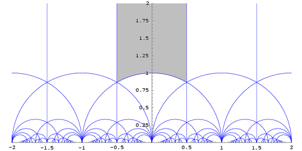
Figure 3: (Color online) Modular transformations generate by $\tau\to\tau+1$ and $\tau\to-1/\tau$ map $\tau$’s in one domain to $\tau$’s in another domain. $\tau$’s in one domain label distinct systems. $\tau$’s in different domains related by a modular transformation describe the same system (up to a coordinate transformation). Each domain has a topology of a sphere minus a point. (The figure comes from Wikipedia.)

Let us assume that the path $\tau(s)$ connects two $\tau$’s, $\tau(0)$ and $\tau(1)$, related by a modular transformation $M=\begin{pmatrix}a&b\\ c&d\end{pmatrix}$: $\tau(1)=\frac{b+d\tau(0)}{a+c\tau(0)}$ (see Fig. 3). We will denote $\tau(0)=\tau$ and $\tau(1)=\tau^{\prime}$. The parallel transportation of the basis $|\gamma;\tau\rangle$ for inverse-mass-matrix $g[\tau(0)]$ gives us a basis $|\gamma;\tau^{\prime}\rangle$ for inverse-mass-matrix $g[\tau(1)]$. Since $\tau=\tau(0)$ and $\tau^{\prime}=\tau(1)$ are related by a modular transformation, $g[\tau(0)]$ and $g[\tau(1)]$ actually describe the same system. The two basis $|\gamma;\tau\rangle$ and $|\gamma;\tau^{\prime}\rangle$ are actually two basis of same space of the degenerate ground states. Thus there is a unitary matrix that relate the two basis

$$|\gamma;\tau^{\prime}\rangle =\hat{U}(M)|\gamma;\tau\rangle$$ (75)

$$U_{\gamma\gamma^{\prime}}(M) =\langle\gamma;\tau|\gamma^{\prime};\tau^{\prime}\rangle=\langle\gamma;\tau|\hat{U}(M)|\gamma^{\prime};\tau\rangle.$$

Such a unitary matrix is the non-Abelian geometric phase for the path $\tau(s)$.

Let us consider a modular transformation generated by $M^{\prime}=\begin{pmatrix}a^{\prime}&b^{\prime}\\ c^{\prime}&d^{\prime}\end{pmatrix}$: $\tau^{\prime}\to\tau^{\prime\prime}=\frac{b^{\prime}+d^{\prime}\tau^{\prime}}{a^{\prime}+c^{\prime}\tau^{\prime}}$. We see that

$$\tau^{\prime\prime}=\frac{b^{\prime}+d^{\prime}\tau^{\prime}}{a^{\prime}+c^{\prime}\tau^{\prime}}=\frac{(ab^{\prime}+bd^{\prime})+(cb^{\prime}+dd^{\prime})\tau}{(aa^{\prime}+bc^{\prime})+(ca^{\prime}+dc^{\prime})\tau}$$ (76)

and the transformation $\tau\to\tau^{\prime\prime}$ is generated by $MM^{\prime}$. From $|\gamma;\tau^{\prime\prime}\rangle=\hat{U}(M^{\prime})|\gamma;\tau^{\prime}\rangle=\hat{U}(M^{\prime})\hat{U}(M)|\gamma;\tau\rangle$, we find that

$$\ \ \ U_{\gamma\gamma^{\prime\prime}}(MM^{\prime})=\langle\gamma;\tau|\gamma^{\prime\prime};\tau^{\prime\prime}\rangle$$ (77)

$$=\sum_{\gamma^{\prime}}\langle\gamma;\tau|\gamma^{\prime};\tau^{\prime}\rangle\langle\gamma^{\prime};\tau^{\prime}|\gamma^{\prime\prime};\tau^{\prime\prime}\rangle=U_{\gamma\gamma^{\prime}}(M)U_{\gamma^{\prime}\gamma^{\prime\prime}}(M^{\prime})$$

Except for its overall phase (which is path dependent), the unitary matrix $U$ is a function of the modular transformation $M$. From eqn. (77), we see that the unitary matrix $U$ form a projective representation of the modular transformation. The projective representation of the modular transformation contains a lot of information (may even all information) of the underlying topological order.

Let us examine $\langle\gamma^{\prime};\tau^{\prime}|\gamma;\tau\rangle$ in eqn. (75) more carefully. Let $\Phi_{\gamma}[\{\boldsymbol{X}_{i}^{I}\}|\tau]$ be ground state wave functions for inverse-mass-matrix $g[\tau]$, and $\Phi_{\gamma}[\{\boldsymbol{X}_{i}\}|\tau^{\prime}]$ be ground state wave functions for inverse-mass-matrix $g[\tau^{\prime}]$. Here $\boldsymbol{X}_{i}=(X^{1,I}_{i},X^{2,I}_{i})$ are the coordinates of the $i^{\text{th}}$ electron in the $I^{\text{th}}$ component. Since $\tau$ and $\tau^{\prime}$ are related by a modular transformation, $\Phi_{\gamma}[\{\boldsymbol{X}_{i}^{I}\}|\tau]$ and $\Phi_{\gamma}[\{\boldsymbol{X}_{i}^{I}\}|\tau^{\prime}]$ are ground state wave function of the same system. However, we cannot directly compare $\Phi_{\gamma}[\{\boldsymbol{X}_{i}^{I}\}|\tau]$ and $\Phi_{\gamma}[\{\boldsymbol{X}_{i}^{I}\}|\tau^{\prime}]$ and calculate the inner product between the two wave functions as

$$\int\prod_{i,I}\hskip 1.0pt\mathrm{d}^{2}\boldsymbol{X}_{i}^{I}\;\Big{[}\Phi_{\gamma}[\{\boldsymbol{X}_{i}^{I}\}|\tau(0)]\Big{]}^{*}\Phi_{\gamma^{\prime}}[\{\boldsymbol{X}_{i}^{I}\}|\tau^{\prime}].$$

The wave function $\Phi_{\gamma}[\{\boldsymbol{X}_{i}^{I}\}|\tau^{\prime}]$ for inverse-mass-matrix $g[\tau^{\prime}]$ can be viewed as the ground state wave function for inverse-mass-matrix $g[\tau]$ only after a coordinate transformation. Let us rename $\boldsymbol{X}$ to $\boldsymbol{X}^{\prime}$ and rewrite $\Phi_{\gamma}[\{\boldsymbol{X}_{i}^{I}\}|\tau^{\prime}]$ as $\Phi_{\gamma}(\{\boldsymbol{X}^{\prime,I}_{i}\}|\tau^{\prime})$. Since the coordinate transformation (72) change $\tau$ to $\tau^{\prime}$, we see that we should really compare $\Phi_{\gamma}(\{\boldsymbol{X}^{\prime,I}_{i}\}|\tau^{\prime})=\Phi_{\gamma}(\{M^{-1}\boldsymbol{X}_{i}^{I}\}|\tau^{\prime})$ with $\Phi_{\gamma}(\{\boldsymbol{X}_{i}^{I}\}|\tau)$. But even $\Phi_{\gamma}(\{\boldsymbol{X}_{i}^{I}\}|\tau)$ and $\Phi_{\gamma}(\{M^{-1}\boldsymbol{X}_{i}^{I}\}|\tau^{\prime})$ cannot be directly compared. This is because the coordinate transformation (71) changes the gauge potential (66) to another gauge equivalent form. We need to perform a $U(1)$ gauge transformation $U_{G}(M)$ to transform the changed gauge potential back to its original form eqn. (66). So only $\Phi_{\gamma}[\{\boldsymbol{X}_{i}^{I}\}|\tau]$ and $U_{G}\Phi_{\gamma}[\{M^{-1}\boldsymbol{X}_{i}^{I}\}|\tau^{\prime}]$ can be directly compared. Therefore, we have

$$\ \ \ U_{\gamma\gamma^{\prime}}(M)$$ (78)

$$=\int_{0}^{1}\prod_{i,I}\hskip 1.0pt\mathrm{d}^{2}\boldsymbol{X}_{i}^{I}\;\Phi^{*}_{\gamma}(\{\boldsymbol{X}_{i}^{I}\}|\tau)U_{G}(M)\Phi_{\gamma^{\prime}}(\{M^{-1}\boldsymbol{X}_{i}^{I}\}|\tau^{\prime})$$

which is eqn. (75) in wave function form. Note that $\tau^{\prime}=\frac{M_{12}+M_{22}\tau}{M_{11}+M_{21}\tau}$.

Let us calculate the gauge transformation $U_{G}(M)$. We note that $\Phi_{\gamma}(\{\boldsymbol{X}^{\prime,I}_{i}\}|\tau^{\prime})$ is the ground state of

$$H^{\prime}=-\sum_{k,I}\frac{1}{2}\sum_{i,j=1,2}\Big{(}\frac{\partial}{\partial X^{\prime i,I}_{k}}-\hskip 1.0pt\mathrm{i}\hskip 1.0ptA^{\prime}_{i}\Big{)}g^{\prime}_{ij}\Big{(}\frac{\partial}{\partial X^{\prime j,I}_{k}}-\hskip 1.0pt\mathrm{i}\hskip 1.0ptA^{\prime}_{j}\Big{)}$$

where $k=1,\cdots,N$ labels the different electrons. In terms of $X^{i}$ (see eqn. (71)), $H^{\prime}$ has a form

$$H^{\prime}=-\sum_{k,I}\frac{1}{2}\sum_{i,j=1,2}\Big{(}\frac{\partial}{\partial X^{i,I}_{k}}-\hskip 1.0pt\mathrm{i}\hskip 1.0pt\tilde{A}_{i}\Big{)}g_{ij}\Big{(}\frac{\partial}{\partial X^{j,I}_{k}}-\hskip 1.0pt\mathrm{i}\hskip 1.0pt\tilde{A}_{j}\Big{)}$$

where

$$\begin{pmatrix}\tilde{A}_{1}\\ \tilde{A}_{2}\\ \end{pmatrix}=\begin{pmatrix}d&-c\\ -b&a\\ \end{pmatrix}\begin{pmatrix}A^{\prime}_{1}\\ A^{\prime}_{2}\\ \end{pmatrix},\ \ \ \ \begin{pmatrix}A^{\prime}_{1}\\ A^{\prime}_{2}\\ \end{pmatrix}=\begin{pmatrix}a&c\\ b&d\\ \end{pmatrix}\begin{pmatrix}\tilde{A}_{1}\\ \tilde{A}_{2}\\ \end{pmatrix}.$$

Since $(A^{\prime}_{1},A^{\prime}_{2})=(-2\pi N_{\phi}X^{\prime 2},0)$, We find that

$$\ \ \ \ (\tilde{A}_{1},\tilde{A}_{2})=(-2\pi N_{\phi}X^{\prime 2}d,\ 2\pi N_{\phi}X^{\prime 2}b)$$

$$=(-2\pi N_{\phi}(-cX^{1}+aX^{2})d,\ 2\pi N_{\phi}(-cX^{1}+aX^{2})b)$$

$U_{G}(M)$ will change $H^{\prime}$ to $H$:

$$\ \ \ \ U_{G}(M)H^{\prime}U_{G}^{\dagger}(M)=H$$

$$=-\sum_{k,I}\frac{1}{2}\sum_{i,j=1,2}\Big{(}\frac{\partial}{\partial X^{i,I}_{k}}-\hskip 1.0pt\mathrm{i}\hskip 1.0ptA_{i}\Big{)}g_{ij}\Big{(}\frac{\partial}{\partial X^{j,I}_{k}}-\hskip 1.0pt\mathrm{i}\hskip 1.0ptA_{j}\Big{)}$$

with $(A_{1},A_{2})=(-2\pi N_{\phi}X^{2},0)$. We find that

$$U_{G}(M;\{\boldsymbol{X}_{i}\}) =\prod_{k,I}u_{G}(M;\boldsymbol{X}_{k}^{I}),$$

$$u_{G}(M;\boldsymbol{X}) =\hskip 1.0pt\mathrm{e}^{\hskip 1.0pt\mathrm{i}\hskip 1.0pt2\pi N_{\phi}[bcX^{1}X^{2}-\frac{cd}{2}(X^{1})^{2}-\frac{ab}{2}(X^{2})^{2}]}.$$ (79)

Note that at $\boldsymbol{X}_{i}=0$, the fixed point of coordinate transformation $\boldsymbol{X}^{\prime}_{i}=M^{-1}\boldsymbol{X}_{i}$, $u_{G}(M;\boldsymbol{X})|_{\boldsymbol{X}=0}=1$.

Eqn. (78) can also be rewritten as a transformation on the wave function $\Phi_{\gamma}(\{\boldsymbol{X}_{i}^{I}\}|\tau)$:

$$\hat{U}(M)\Phi_{\gamma}(\{\boldsymbol{X}_{i}^{I}\}|\tau) =U_{G}(M)\Phi_{\gamma}(\{\boldsymbol{X}^{\prime,I}_{i}\}|\tau^{\prime})$$

$$=U_{G}(M)\Phi_{\gamma}(\{M^{-1}\boldsymbol{X}_{i}^{I}\}|\tau^{\prime})$$

$$=\Phi_{\gamma^{\prime}}(\{\boldsymbol{X}_{i}^{I}\}|\tau)U_{\gamma^{\prime}\gamma}(M).$$ (80)

where $\tau^{\prime}=\frac{M_{12}+M_{22}\tau}{M_{11}+M_{21}\tau}$. Let

$$M_{T}=\begin{pmatrix}1&1\\ 0&1\end{pmatrix},\ \ \ \ \ M_{S}=\begin{pmatrix}0&-1\\ 1&0\end{pmatrix}.$$

Since $\Phi_{\gamma}(\{\boldsymbol{X}_{i}^{I}\}|\tau)$ has a form

$$\Phi_{\gamma}(\{\boldsymbol{X}_{i}^{I}\}|\tau)=f_{\gamma}(\{X^{1,I}_{i}+\tau X^{2,I}_{i}\}|\tau)e^{\hskip 1.0pt\mathrm{i}\hskip 1.0pt\pi\tau N_{\phi}\sum_{i}(X^{2,I}_{i})^{2}}$$

where $f_{\gamma}(\{z_{i}^{I}\}|\tau)$ is a holomorphic function, we can express the action of $\hat{U}(M_{T})$ and $\hat{U}(M_{S})$ on $\Phi_{\gamma}(\{\boldsymbol{X}_{i}^{I}\}|\tau)$ as

$$\hat{U}(M_{T})\Phi_{\gamma}(\{\boldsymbol{X}_{i}^{I}\}|\tau)=U_{G}(M_{T})\Phi_{\gamma}(\{X^{1,I}_{i}-X^{2,I}_{i},X^{2,I}_{i}\}|\tau+1)$$

$$=U_{G}(M_{T})f_{\gamma}(\{(X^{1,I}_{i}-X^{2,I}_{i})+(\tau+1)X^{2,I}_{i}\}|\tau+1)e^{\hskip 1.0pt\mathrm{i}\hskip 1.0pt\pi(\tau+1)N_{\phi}\sum_{i,I}(X^{2,I}_{i})^{2}}$$

$$=\hskip 1.0pt\mathrm{e}^{-\hskip 1.0pt\mathrm{i}\hskip 1.0pt\pi N_{\phi}\sum_{i,I}(X^{2,I}_{i})^{2}}f_{\gamma}(\{z_{i}^{I}\}|\tau+1)e^{\hskip 1.0pt\mathrm{i}\hskip 1.0pt\pi(\tau+1)N_{\phi}\sum_{i,I}(X^{2,I}_{i})^{2}}=f_{\gamma}(\{z_{i}^{I}\}|\tau+1)e^{\hskip 1.0pt\mathrm{i}\hskip 1.0pt\pi\tau N_{\phi}\sum_{i,I}(X^{2,I}_{i})^{2}},$$

and

$$\hat{U}(M_{S})\Phi_{\gamma}(\{\boldsymbol{X}_{i}^{I}\}|\tau)=U_{G}(M_{S})\Phi_{\gamma}(\{X_{i}^{2,I},-X_{i}^{1,I}\}|\frac{-1}{\tau})=U_{G}(M_{T})f_{\gamma}(\{X^{2,I}_{i}-(\frac{-1}{\tau})X^{1,I}_{i}\}|\frac{-1}{\tau})e^{\hskip 1.0pt\mathrm{i}\hskip 1.0pt\pi(\frac{-1}{\tau})N_{\phi}\sum_{i,I}(X^{1,I}_{i})^{2}}$$

$$=\hskip 1.0pt\mathrm{e}^{-2\hskip 1.0pt\mathrm{i}\hskip 1.0pt\pi N_{\phi}\sum_{i,I}X^{1,I}_{i}X^{2,I}_{i}}f_{\gamma}(\{z_{i}/\tau\}|\frac{-1}{\tau})e^{-\hskip 1.0pt\mathrm{i}\hskip 1.0pt\pi N_{\phi}\sum_{i,I}(X^{1,I}_{i})^{2}/\tau}=f_{\gamma}(\{z_{i}^{I}/\tau\}|\frac{-1}{\tau})\hskip 1.0pt\mathrm{e}^{-\hskip 1.0pt\mathrm{i}\hskip 1.0pt\pi N_{\phi}\sum_{i,I}(z_{i}^{I})^{2}/\tau}e^{\hskip 1.0pt\mathrm{i}\hskip 1.0pt\pi\tau N_{\phi}\sum_{i,I}(X^{2,I}_{i})^{2}},$$

where $z_{i}^{I}=X^{1,I}_{i}+\tau X^{2,I}_{i}$. We see that the action of operator $\hat{U}(M)$ can be expressed as the action of another operator $\hat{\tilde{U}}(M)$ on $f_{\gamma}(\{\boldsymbol{X}_{i}^{I}\}|\tau)$, where

$$\hat{\tilde{U}}(M)=e^{-\hskip 1.0pt\mathrm{i}\hskip 1.0pt\pi\tau N_{\phi}\sum_{i}(X^{2,I}_{i})^{2}}\hat{U}(M)e^{\hskip 1.0pt\mathrm{i}\hskip 1.0pt\pi\tau N_{\phi}\sum_{i}(X^{2,I}_{i})^{2}}.$$

We find

$$\hat{\tilde{U}}(M_{T})f_{\gamma}(\{z_{i}^{I}\}|\tau) =f_{\gamma}(\{z_{i}^{I}\}|\tau+1)$$

$$=f_{\gamma^{\prime}}(\{z_{i}^{I}\}|\tau)U_{\gamma^{\prime}\gamma}(M_{T}),$$

$$\hat{\tilde{U}}(M_{S})f_{\gamma}(\{z_{i}^{I}\}|\tau) =f_{\gamma}(\{z_{i}^{I}/\tau\}|\frac{-1}{\tau})\hskip 1.0pt\mathrm{e}^{-\hskip 1.0pt\mathrm{i}\hskip 1.0pt\pi N_{\phi}\sum_{i,I}(z_{i}^{I})^{2}/\tau}$$

$$=f_{\gamma^{\prime}}(\{z_{i}^{I}\}|\tau)U_{\gamma^{\prime}\gamma}(M_{S}).$$ (81)

We may use this result to calculate $U_{\gamma\gamma^{\prime}}(M)$.

In the above, we have assumed that $\Phi_{\gamma}(\tau)$ form an orthonormal basis $\langle\Phi_{\gamma}(\tau)|\Phi_{\gamma^{\prime}}(\tau)\rangle=\delta_{\gamma\gamma^{\prime}}$. In this case, $U_{\gamma\gamma^{\prime}}(M)$ is an unitary matrix. However, it is more convenient to choose “chiral normalization” such that $\langle\Phi_{\gamma}(\tau)|\Phi_{\gamma^{\prime}}(\tau)\rangle\propto\delta_{\gamma\gamma^{\prime}}$ and that $\Phi_{\gamma}(\tau)$ is a holomorphic function of $\tau$. We will choose such a “chiral normalization” in this paper.

To summarize, there are two kinds of deformation loops $\tau(s)$. If $\tau(0)=\tau(1)$, the deformation loop is contactable [ie we can deform the loop to a point, or in other words we can continuously deform the function $\tau(s)$ to a constant function $\tau(s)=\tau(0)=\tau(1)$]. For a contactable loop, the associated non-Abelian geometric phase is actually a $U(1)$ phase $U_{\gamma\gamma^{\prime}}=\hskip 1.0pt\mathrm{e}^{\hskip 1.0pt\mathrm{i}\hskip 1.0pt\varphi}\delta_{\gamma\gamma^{\prime}}$. where $\varphi$ is path dependent. If $\tau(0)$ and $\tau(1)$ are related by a modular transformation, the deformation loop is non-contactable. Then the associated non-Abelian geometric phase is non-trivial. If two non-contactable loops can be deformed into each other continuously, then the two loops only differ by a contactable loop. The associated non-Abelian geometric phases will only differ by a an overall $U(1)$ phase. Thus, up to an overall $U(1)$ phase, the non-Abelian geometric phases $U_{\gamma\gamma^{\prime}}$ of a topologically ordered state are determined by the modular transformation $\tau\to\tau^{\prime}=\frac{b+d\tau}{a+c\tau}$. We also show that we can use the parallel transportation to defined a system of basis $\Phi_{\gamma}(\{\boldsymbol{X}_{i}\}|\tau)$ for all inverse-mass-matrices labeled by $\tau$.

V.1 Calculation for Abelian states

For the Abelian FQH states, we have already introduced a system of basis for the degenerate ground states for each inverse-mass-matrix $g(\tau)$: $|\boldsymbol{\alpha};\tau\rangle=\Phi^{\boldsymbol{\alpha}}_{K}(\{\boldsymbol{X}^{I}_{i}\}|\tau)$ (see eqn. (50), eqn. (51), and eqn. (54)). It appears that such a system of basis happen to be a system of orthogonal basis that are related by the parallel transformation (up to an overall phase), ie the basis satisfy

$$\langle\boldsymbol{\beta};\tau|\frac{\hskip 1.0pt\mathrm{d}}{\hskip 1.0pt\mathrm{d}\tau}|\boldsymbol{\alpha};\tau\rangle\propto\delta_{\boldsymbol{\alpha}\boldsymbol{\beta}},\ \ \ \ \langle\boldsymbol{\beta};\tau|\frac{\hskip 1.0pt\mathrm{d}}{\hskip 1.0pt\mathrm{d}\tau^{*}}|\boldsymbol{\alpha};\tau\rangle\propto\delta_{\boldsymbol{\alpha}\boldsymbol{\beta}}.$$ (82)

One way to see this result is to note that the wave function $\Phi^{\boldsymbol{\alpha}}_{K}(\{\boldsymbol{X}^{I}_{i}\}|\tau)$ factorizes as a product of center-of-mass wave function and relative-motion wave function (see eqn. (54)). So up to the over all $U(1)$ phase, the non-Abelian geometric phases are determined by the center-of-mass wave function only, because the relative-motion wave function does not depend on $\boldsymbol{\alpha}$. If we only look at the center-of-mass wave functions $\Phi^{\boldsymbol{\alpha}}_{K,c}(\boldsymbol{Z}|\tau)$, one can show that they form a system of orthogonal basis (parametrized by $\tau$) that are related by the parallel transformation (up to an overall phase).

So if we choose the basis for the degenerate ground states as $|\boldsymbol{\alpha};\tau\rangle=\Phi^{\boldsymbol{\alpha}}_{K}(\{\boldsymbol{X}^{I}_{i}\}|\tau)$ (see eqn. (50), eqn. (51), and eqn. (54)), then we can use eqn. (V) to calculate the non-Abelian geometric phases associated with the two generators $T:\tau\to\tau+1$ and $S:\tau\to\-1/\tau$ of the modular transformations.

Let us consider the bosonic electrons. From eqn. (54) and eqn. (50), we see that

$$f^{(\boldsymbol{\alpha})}(\{z^{I}_{i}\}|\tau)=\eta^{-\kappa}(\tau)f^{(\boldsymbol{\alpha},0)}(\{Z^{I}\}|\tau)\times$$ (83)

$$\ \ \ \ \ \ \ \ \ \ \ \Big{\{}\prod_{I<J}\prod_{i,j}\eta^{-K_{IJ}}(\tau)\theta^{K_{IJ}}_{11}(z^{I}_{i}-z^{J}_{j}|\tau)\Big{\}}\times$$

$$\ \ \ \ \ \ \ \ \ \ \ \Big{\{}\prod_{I}\prod_{i<j}\eta^{-K_{II}}(\tau)\theta^{K_{II}}_{11}(z^{I}_{i}-z^{I}_{j}|\tau)\Big{\}}$$

Using eqn. (B), eqn. (108), and eqn. (53), we obtain

$$f^{(\boldsymbol{\alpha})}(\{z^{I}_{i}\}|\tau+1)=\hskip 1.0pt\mathrm{e}^{\frac{1}{6}\hskip 1.0pt\mathrm{i}\hskip 1.0pt\pi[\sum_{I<J}K_{IJ}N^{I}N^{J}+\sum_{I}\frac{K_{II}}{2}N_{I}(N_{I}-1)]}\times$$

$$\ \ \ \ \ \ \ \ \ \ \ \ \ \ \ \ \ \ \ \ \ \ \ \ \ \ \ \ \ \hskip 1.0pt\mathrm{e}^{\hskip 1.0pt\mathrm{i}\hskip 1.0pt\pi(\boldsymbol{\alpha}^{T}K\boldsymbol{\alpha}-\frac{1}{12}\kappa)}f^{(\boldsymbol{\alpha})}(\{z^{I}_{i}\}|\tau)$$

$$=\hskip 1.0pt\mathrm{e}^{\frac{1}{12}\hskip 1.0pt\mathrm{i}\hskip 1.0pt\pi(\boldsymbol{N}^{T}K\boldsymbol{N}-\boldsymbol{\kappa}^{T}\boldsymbol{N})}\hskip 1.0pt\mathrm{e}^{\hskip 1.0pt\mathrm{i}\hskip 1.0pt\pi(\boldsymbol{\alpha}^{T}K\boldsymbol{\alpha}-\frac{1}{12}\kappa)}f^{(\boldsymbol{\alpha})}(\{z^{I}_{i}\}|\tau)$$ (84)

where $\boldsymbol{N}$ is a column vector with component $N_{I}$ and $\boldsymbol{\kappa}$ is a column vector with component $K_{II}$ (see eqn. (IV.2)). Therefore, from the definition eqn. (V), we find that

$$\Phi^{\boldsymbol{\alpha}}_{K}(\{\tilde{X}^{1,I}_{i},\tilde{X}^{2,I}_{i}\};\tau+1)=\hskip 1.0pt\mathrm{e}^{\hskip 1.0pt\mathrm{i}\hskip 1.0pt\pi N_{\phi}\sum_{i,I}(X_{i}^{2,I})^{2}}\times$$ (85)

$$\ \ \ \hskip 1.0pt\mathrm{e}^{\frac{1}{12}\hskip 1.0pt\mathrm{i}\hskip 1.0pt\pi(\boldsymbol{N}^{T}K\boldsymbol{N}-\boldsymbol{\kappa}^{T}\boldsymbol{N})}\hskip 1.0pt\mathrm{e}^{\hskip 1.0pt\mathrm{i}\hskip 1.0pt\pi(\boldsymbol{\alpha}^{T}K\boldsymbol{\alpha}-\frac{1}{12}\kappa)}\Phi^{\boldsymbol{\alpha}}_{K}(\{X^{1,I}_{i},X^{2,I}_{i}\};\tau)$$

where

$$\tilde{X}^{1,I}_{i}+(\tau+1)\tilde{X}^{2,I}_{i}=X^{1,I}_{i}+\tau X^{2,I}_{i}$$ (86)

or

$$X^{1,I}_{i}=\tilde{X}^{1,I}_{i}+\tilde{X}^{2,I}_{i},\ \ \ \ X^{2,I}_{i}=\tilde{X}^{2,I}_{i}.$$ (87)

Using eqn. (122), eqn. (109), and eqn. (53), we obtain that

$$f^{(\boldsymbol{\alpha})}(\{z^{I}_{i}/\tau\}|-1/\tau)=(-)^{(\boldsymbol{N}^{T}K\boldsymbol{N}-\boldsymbol{\kappa}^{T}\boldsymbol{N})/2}\times$$

$$\ \ \ \hskip 1.0pt\mathrm{e}^{\hskip 1.0pt\mathrm{i}\hskip 1.0pt\frac{\pi}{\tau}[\sum_{I<J;i,j}K_{IJ}(z^{I}_{i}-z^{J}_{j})^{2}+\sum_{I;i<j}K_{II}(z^{I}_{i}-z^{I}_{j})^{2}]}\times$$ (88)

$$\ \ \ \hskip 1.0pt\mathrm{e}^{\hskip 1.0pt\mathrm{i}\hskip 1.0pt\pi\boldsymbol{Z}^{T}K\boldsymbol{Z}/\tau}\sum_{\boldsymbol{\beta}\in UC}\frac{\hskip 1.0pt\mathrm{e}^{-\hskip 1.0pt\mathrm{i}\hskip 1.0pt2\pi\boldsymbol{\beta}^{T}K\boldsymbol{\alpha}}}{\sqrt{\det(K)}}f^{(\boldsymbol{\beta})}(\{z^{I}_{i}\}|\tau)$$

Note that

$$\ \ \ \sum_{I<J;i,j}K_{IJ}(z^{I}_{i}-z^{J}_{j})^{2}+\sum_{I;i<j}K_{II}(z^{I}_{i}-z^{I}_{j})^{2}$$

$$=\frac{1}{2}\sum_{I,J;i,j}K_{IJ}(z^{I}_{i}-z^{J}_{j})^{2}=N_{\phi}\sum_{I,i}(z^{I}_{i})^{2}-\sum_{I,J;i,j}K_{IJ}z^{I}_{i}z^{J}_{j}$$

$$=N_{\phi}\sum_{I,i}(z^{I}_{i})^{2}-\boldsymbol{Z}^{T}K\boldsymbol{Z},$$ (89)

where we have used $N_{\phi}=K_{IJ}N_{J}$. Therefore, we have

$$\ \ \ f^{(\boldsymbol{\alpha})}(\{z^{I}_{i}/\tau\}|-1/\tau)\hskip 1.0pt\mathrm{e}^{-\hskip 1.0pt\mathrm{i}\hskip 1.0pt\frac{\pi}{\tau}N_{\phi}\sum_{I,i}(z^{I}_{i})^{2}}$$

$$=(-)^{(\boldsymbol{N}^{T}K\boldsymbol{N}-\boldsymbol{\kappa}^{T}\boldsymbol{N})/2}\sum_{\boldsymbol{\beta}\in UC}\frac{\hskip 1.0pt\mathrm{e}^{-\hskip 1.0pt\mathrm{i}\hskip 1.0pt2\pi\boldsymbol{\beta}^{T}K\boldsymbol{\alpha}}}{\sqrt{\det(K)}}f^{(\boldsymbol{\beta})}(\{z^{I}_{i}\}|\tau)$$

From the definition eqn. (V), we find that

$$\Phi^{\boldsymbol{\alpha}}_{K}(\{\tilde{X}^{1,I}_{i},\tilde{X}^{2,I}_{i}\};-1/\tau)=\hskip 1.0pt\mathrm{e}^{2\hskip 1.0pt\mathrm{i}\hskip 1.0pt\pi N_{\phi}\sum_{i,I}X_{i}^{1,I}X_{i}^{2,I}}\times$$ (90)

$$(-)^{(\boldsymbol{N}^{T}K\boldsymbol{N}-\boldsymbol{\kappa}^{T}\boldsymbol{N})/2}\sum_{\boldsymbol{\beta}\in UC}\frac{\hskip 1.0pt\mathrm{e}^{-\hskip 1.0pt\mathrm{i}\hskip 1.0pt2\pi\boldsymbol{\beta}^{T}K\boldsymbol{\alpha}}}{\sqrt{\det(K)}}\Phi^{\boldsymbol{\beta}}_{K}(\{X^{1,I}_{i},X^{2,I}_{i}\};\tau)$$

where

$$\tilde{X}^{1,I}_{i}-\frac{1}{\tau}\tilde{X}^{2,I}_{i}=(X^{1,I}_{i}+\tau X^{2,I}_{i})/\tau$$ (91)

or

$$X^{1,I}_{i}=-\tilde{X}^{2,I}_{i},\ \ \ \ X^{2,I}_{i}=\tilde{X}^{1,I}_{i}.$$ (92)

So for bosonic electrons, the non-Abelian geometric phases are described by the following generators of (projective) representation of modular group

$$U_{\boldsymbol{\alpha}\boldsymbol{\beta}}(M_{T}) =\hskip 1.0pt\mathrm{e}^{\frac{\hskip 1.0pt\mathrm{i}\hskip 1.0pt\pi}{12}(\boldsymbol{N}^{T}K\boldsymbol{N}-\boldsymbol{\kappa}^{T}\boldsymbol{N})}\hskip 1.0pt\mathrm{e}^{\hskip 1.0pt\mathrm{i}\hskip 1.0pt\pi(\boldsymbol{\alpha}^{T}K\boldsymbol{\alpha}-\frac{1}{12}\kappa)}\delta_{\boldsymbol{\alpha}\boldsymbol{\beta}}$$

$$U_{\boldsymbol{\alpha}\boldsymbol{\beta}}(M_{S}) =(-)^{(\boldsymbol{N}^{T}K\boldsymbol{N}-\boldsymbol{\kappa}^{T}\boldsymbol{N})/2}\frac{\hskip 1.0pt\mathrm{e}^{-\hskip 1.0pt\mathrm{i}\hskip 1.0pt2\pi\boldsymbol{\beta}^{T}K\boldsymbol{\alpha}}}{\sqrt{\det(K)}}$$ (93)

Now we consider the fermionic electrons. From eqn. (54) and eqn. (51), we see that

$$f^{(\boldsymbol{\alpha})}(\{z^{I}_{i}\}|\tau)=\eta^{-\kappa}(\tau)f^{(\boldsymbol{\alpha},K^{-1}\boldsymbol{\kappa}/2)}(\{Z^{I}\}|\tau)\times$$ (94)

$$\ \ \ \ \ \Big{\{}\prod_{I<J}\prod_{i,j}\eta^{-K_{IJ}}(\tau)\theta^{K_{IJ}}_{11}(z^{I}_{i}-z^{J}_{j}|\tau)\Big{\}}\times$$

$$\ \ \ \ \ \Big{\{}\prod_{I}\prod_{i<j}\eta^{-K_{II}}(\tau)\theta^{K_{II}}_{11}(z^{I}_{i}-z^{I}_{j}|\tau)\Big{\}}$$

Using eqn. (B) and eqn. (108), we obtain that

$$f^{(\boldsymbol{\alpha})}(\{z^{I}_{i}\}|\tau+1)=\hskip 1.0pt\mathrm{e}^{\frac{1}{12}\hskip 1.0pt\mathrm{i}\hskip 1.0pt\pi(\boldsymbol{N}^{T}K\boldsymbol{N}-\boldsymbol{\kappa}^{T}\boldsymbol{N}-\kappa)}\times$$

$$\ \ \ \ \hskip 1.0pt\mathrm{e}^{\hskip 1.0pt\mathrm{i}\hskip 1.0pt\pi(\boldsymbol{\alpha}+\frac{1}{2}K^{-1}\boldsymbol{\kappa})^{T}K(\boldsymbol{\alpha}+\frac{1}{2}K^{-1}\boldsymbol{\kappa})}f^{(\boldsymbol{\alpha})}(\{z^{I}_{i}\}|\tau).$$ (95)

Using eqn. (B) and eqn. (109), we obtain

$$\ \ \ f^{(\boldsymbol{\alpha})}(\{z^{I}_{i}/\tau\}|-1/\tau)\hskip 1.0pt\mathrm{e}^{-\hskip 1.0pt\mathrm{i}\hskip 1.0pt\frac{\pi}{\tau}N_{\phi}\sum_{I,i}(z^{I}_{i})^{2}}$$

$$=(-)^{(\boldsymbol{N}^{T}K\boldsymbol{N}-\boldsymbol{\kappa}^{T}\boldsymbol{N})/2}\hskip 1.0pt\mathrm{e}^{\frac{1}{2}\hskip 1.0pt\mathrm{i}\hskip 1.0pt\pi\boldsymbol{\kappa}^{T}K^{-1}\boldsymbol{\kappa}}\times$$

$$\ \ \ \ \ \sum_{\boldsymbol{\beta}\in UC}\frac{\hskip 1.0pt\mathrm{e}^{-\hskip 1.0pt\mathrm{i}\hskip 1.0pt2\pi(\boldsymbol{\beta}^{T}K\boldsymbol{\alpha}+\boldsymbol{\beta}^{T}\boldsymbol{\kappa})}}{\sqrt{\det(K)}}f^{(\boldsymbol{\beta})}(\{z^{I}_{i}\}|\tau)$$

So for fermionic electrons, the non-Abelian geometric phases are described by the following generators of (projective) representation of modular group

$$U_{\boldsymbol{\alpha}\boldsymbol{\beta}}(M_{T}) =\hskip 1.0pt\mathrm{e}^{\frac{1}{12}\hskip 1.0pt\mathrm{i}\hskip 1.0pt\pi(\boldsymbol{N}^{T}K\boldsymbol{N}-\boldsymbol{\kappa}^{T}\boldsymbol{N}-\kappa)}\times$$

$$\ \ \ \ \hskip 1.0pt\mathrm{e}^{\hskip 1.0pt\mathrm{i}\hskip 1.0pt\pi(\boldsymbol{\alpha}+\frac{1}{2}K^{-1}\boldsymbol{\kappa})^{T}K(\boldsymbol{\alpha}+\frac{1}{2}K^{-1}\boldsymbol{\kappa})}\delta_{\boldsymbol{\alpha}\boldsymbol{\beta}}$$

$$U_{\boldsymbol{\alpha}\boldsymbol{\beta}}(M_{S}) =(-)^{(\boldsymbol{N}^{T}K\boldsymbol{N}-\boldsymbol{\kappa}^{T}\boldsymbol{N})/2}\times$$

$$\ \ \ \ \hskip 1.0pt\mathrm{e}^{\frac{1}{2}\hskip 1.0pt\mathrm{i}\hskip 1.0pt\pi\boldsymbol{\kappa}^{T}K^{-1}\boldsymbol{\kappa}}\frac{\hskip 1.0pt\mathrm{e}^{-\hskip 1.0pt\mathrm{i}\hskip 1.0pt2\pi(\boldsymbol{\alpha}^{T}K\boldsymbol{\beta}+\boldsymbol{\beta}^{T}\boldsymbol{\kappa})}}{\sqrt{\det(K)}}$$ (96)

VI Summary

Let us summarize the results obtained in this paper. For an Abelian FQH state $(K,\boldsymbol{q})$ on a torus, the ground state degeneracy is given by $|\det(K)|$. The degenerate ground states $|\boldsymbol{\alpha}\rangle$ can be labeled by the $\kappa$ dimensional vectors $\boldsymbol{\alpha}$ in the $\kappa$ dimensional unit cube, where $\kappa$ is the dimension of $K$ and $\boldsymbol{\alpha}$ satisfy the quantization condition

$$K\boldsymbol{\alpha}=\text{integer vectors}.$$

$\boldsymbol{\alpha}$’s that differ by an integer vector correspond to the same state.

Assume that the torus is a square of size 1: $(X_{1},X_{2})\sim(X_{1}+1,X_{2})\sim(X_{1},X_{2}+1)$ with $N_{\phi}$ magnetic flux quanta. To simplify our result, we will assume $N_{\phi}=$ even (see eqn. (45)). The Hamiltonian commutes with $T^{(N)}_{1}$ and $T^{(N)}_{2}$, where $T^{(N)}_{1}$ generates translation $(X_{1},X_{2})\to(X_{1}+\frac{1}{N_{\phi}},X_{2})$ and $T^{(N)}_{2}$ generates translation $(X_{1},X_{2})\to(X_{1},X_{2}+\frac{1}{N_{\phi}})$. $T^{(N)}_{1}$ and $T^{(N)}_{2}$ satisfy the Heisenberg algebra

$$T^{(N)}_{1}T^{(N)}_{2}=\hskip 1.0pt\mathrm{e}^{\hskip 1.0pt\mathrm{i}\hskip 1.0pt2\pi\frac{N}{N_{\phi}}}T^{(N)}_{2}T^{(N)}_{1}$$

where $N$ is the total number of electrons. The degenerate ground states $|\boldsymbol{\alpha}\rangle$ form a representation of the Heisenberg algebra: for bosonic electrons,

$$T^{(N)}_{1}|\boldsymbol{\alpha}\rangle =\hskip 1.0pt\mathrm{e}^{\hskip 1.0pt\mathrm{i}\hskip 1.0pt2\pi\boldsymbol{q}^{T}\boldsymbol{\alpha}}|\boldsymbol{\alpha}\rangle,$$

$$T^{(N)}_{2}|\boldsymbol{\alpha}\rangle =|\boldsymbol{\alpha}+K^{-1}\boldsymbol{q}\rangle,$$ (97)

and for fermionic electrons,

$$T^{(N)}_{1}|\boldsymbol{\alpha}\rangle =(-)^{\boldsymbol{\kappa}^{T}\boldsymbol{q}}\hskip 1.0pt\mathrm{e}^{\hskip 1.0pt\mathrm{i}\hskip 1.0pt2\pi\boldsymbol{q}^{T}\boldsymbol{\alpha}}|\boldsymbol{\alpha}\rangle,$$

$$T^{(N)}_{2}|\boldsymbol{\alpha}\rangle =(-)^{\boldsymbol{\kappa}^{T}\boldsymbol{q}}|\boldsymbol{\alpha}+K^{-1}\boldsymbol{q}\rangle.$$ (98)

For generic inverse-mass-matrix $g$ in eqn. (67), the degenerate ground states have a $\tau$ dependence $|\boldsymbol{\alpha};\tau\rangle$. By deforming $\tau$ to $\tau^{\prime}=\frac{b+a\tau}{d+c\tau}$, we can obtain a non-Abelian geometric phase $U(\tau\to\tau^{\prime})$. $U(\tau\to\tau^{\prime})$’s form a projective representation of the modular group.

For two generators of the modular group $S=U(\tau\to-1/\tau)=U(M_{S})$ and $T=U(\tau\to\tau+1)=U(M_{T})$, we find that, for bosonic electrons (see eqn. (V.1))

$$T_{\boldsymbol{\alpha}\boldsymbol{\beta}} =\hskip 1.0pt\mathrm{e}^{\frac{\hskip 1.0pt\mathrm{i}\hskip 1.0pt\pi}{12}(\boldsymbol{N}^{T}K\boldsymbol{N}-\boldsymbol{\kappa}^{T}\boldsymbol{N})}\hskip 1.0pt\mathrm{e}^{\hskip 1.0pt\mathrm{i}\hskip 1.0pt\pi(\boldsymbol{\alpha}^{T}K\boldsymbol{\alpha}-\frac{1}{12}\kappa)}\delta_{\boldsymbol{\alpha}\boldsymbol{\beta}}$$

$$S_{\boldsymbol{\alpha}\boldsymbol{\beta}} =(-)^{(\boldsymbol{N}^{T}K\boldsymbol{N}-\boldsymbol{\kappa}^{T}\boldsymbol{N})/2}\sum_{\boldsymbol{\beta}\in UC}\frac{\hskip 1.0pt\mathrm{e}^{-\hskip 1.0pt\mathrm{i}\hskip 1.0pt2\pi\boldsymbol{\beta}^{T}K\boldsymbol{\alpha}}}{\sqrt{\det(K)}}$$ (99)

and for fermionic electrons (see eqn. (V.1))

$$T_{\boldsymbol{\alpha}\boldsymbol{\beta}} =\hskip 1.0pt\mathrm{e}^{\frac{1}{12}\hskip 1.0pt\mathrm{i}\hskip 1.0pt\pi(\boldsymbol{N}^{T}K\boldsymbol{N}-\boldsymbol{\kappa}^{T}\boldsymbol{N}-\kappa)}\times$$

$$\ \ \ \ \hskip 1.0pt\mathrm{e}^{\hskip 1.0pt\mathrm{i}\hskip 1.0pt\pi(\boldsymbol{\alpha}+\frac{1}{2}K^{-1}\boldsymbol{\kappa})^{T}K(\boldsymbol{\alpha}+\frac{1}{2}K^{-1}\boldsymbol{\kappa})}\delta_{\boldsymbol{\alpha}\boldsymbol{\beta}}$$

$$S_{\boldsymbol{\alpha}\boldsymbol{\beta}} =(-)^{(\boldsymbol{N}^{T}K\boldsymbol{N}-\boldsymbol{\kappa}^{T}\boldsymbol{N})/2}\times$$

$$\ \ \ \ \hskip 1.0pt\mathrm{e}^{\frac{1}{2}\hskip 1.0pt\mathrm{i}\hskip 1.0pt\pi\boldsymbol{\kappa}^{T}K^{-1}\boldsymbol{\kappa}}\frac{\hskip 1.0pt\mathrm{e}^{-\hskip 1.0pt\mathrm{i}\hskip 1.0pt2\pi(\boldsymbol{\alpha}^{T}K\boldsymbol{\beta}+\boldsymbol{\beta}^{T}\boldsymbol{\kappa})}}{\sqrt{\det(K)}}$$ (100)

where $\boldsymbol{\kappa}^{T}=(K^{11},K^{22},\cdots,K^{\kappa\kappa})$ is two times the spin vector of the Abelian FQH state.Wen (1995) We see that the $S$-matrix contains information about the mutual statistics $2\pi\boldsymbol{\alpha}^{T}K\boldsymbol{\beta}$ between the quasi-particles labeled by $\boldsymbol{\alpha}$ and $\boldsymbol{\beta}$, while the $T$-matrix contains information about the statistics $\pi\boldsymbol{\alpha}^{T}K\boldsymbol{\alpha}$ of the quasi-particle labeled by $\boldsymbol{\alpha}$.Wen (1990); Keski-Vakkuri and Wen (1993)

We have calculated the above unitary matrices $S,T$ carefully such that the over all $U(1)$ phase is meanful. We have achieve this by choosing the degenerate ground state wave functions on torus to be (1) holomorphic functions of $\tau$ and (2) modular forms of level zero (the $\tau\to-1/\tau$ modular transformation do not have the $\sqrt{-\hskip 1.0pt\mathrm{i}\hskip 1.0pt\tau}$ factor). (1) is achieved by choosing proper gauge for the background magnetic field, and (2) is achieved by including proper powers of Dedekind $\eta(\tau)$ function in the ground state wave functions (see eqn. (50) and eqn. (54)). So the amibguity of the ground state wave function is only a constant factor that is independent of $\tau$. Such a constant factor is a unitary matrix $W$ that is independent of $\tau$. So the ambiguity of $T,S$ is

$$T\to WTW^{\dagger},\ \ \ \ S\to WSW^{\dagger}.$$ (101)

We note that $M_{S}$ generates a 90^∘ rotation (see eqn. (72)). Also when $\tau=\hskip 1.0pt\mathrm{i}\hskip 1.0pt$, the torus has a 90^∘ symmetry. So $S=R_{90^{\circ}}$ is the generator of the 90^∘ rotation among the degenerate ground states when $\tau=\hskip 1.0pt\mathrm{i}\hskip 1.0pt$. We also note that $M_{S}M_{T}=\begin{pmatrix}0&-1\\ 1&1\end{pmatrix}$ and $(M_{S}M_{T})^{3}=\begin{pmatrix}-1&0\\ 0&-1\end{pmatrix}$ which is a 180^∘ rotation (see eqn. (72)). So $M_{S}M_{T}$ generates a 60^∘ rotation. When $\tau=\hskip 1.0pt\mathrm{e}^{\hskip 1.0pt\mathrm{i}\hskip 1.0pt\pi/3}$, the torus has a 60^∘ symmetry. So $U(M_{S}M_{T})=U(M_{S})U(M_{T})=ST=R_{60^{\circ}}$ is the generator of the 60^∘ rotation among the degenerate ground states when $\tau=\hskip 1.0pt\mathrm{e}^{\hskip 1.0pt\mathrm{i}\hskip 1.0pt\pi/3}$. We find that, for bosonic electrons

$$R_{60^{\circ}} =\hskip 1.0pt\mathrm{e}^{\frac{7}{12}\hskip 1.0pt\mathrm{i}\hskip 1.0pt\pi(\boldsymbol{N}^{T}K\boldsymbol{N}-\boldsymbol{\kappa}^{T}\boldsymbol{N})}\hskip 1.0pt\mathrm{e}^{-\frac{1}{12}\hskip 1.0pt\mathrm{i}\hskip 1.0pt\pi\kappa}\frac{\hskip 1.0pt\mathrm{e}^{\hskip 1.0pt\mathrm{i}\hskip 1.0pt\pi(\boldsymbol{\beta}-2\boldsymbol{\alpha})^{T}K\boldsymbol{\beta}}}{\sqrt{\det(K)}}$$ (102)

and for fermionic electrons

$$R_{60^{\circ}} =\hskip 1.0pt\mathrm{e}^{\frac{7}{12}\hskip 1.0pt\mathrm{i}\hskip 1.0pt\pi(\boldsymbol{N}^{T}K\boldsymbol{N}-\boldsymbol{\kappa}^{T}\boldsymbol{N})}\hskip 1.0pt\mathrm{e}^{-\frac{1}{12}\hskip 1.0pt\mathrm{i}\hskip 1.0pt\pi\kappa}\hskip 1.0pt\mathrm{e}^{\frac{1}{2}\hskip 1.0pt\mathrm{i}\hskip 1.0pt\pi\boldsymbol{\kappa}^{T}K^{-1}\boldsymbol{\kappa}}\times$$

$$\ \ \ \ \frac{\hskip 1.0pt\mathrm{e}^{-\hskip 1.0pt\mathrm{i}\hskip 1.0pt2\pi(\boldsymbol{\alpha}^{T}K\boldsymbol{\beta}+\boldsymbol{\beta}^{T}\boldsymbol{\kappa})}}{\sqrt{\det(K)}}\hskip 1.0pt\mathrm{e}^{\hskip 1.0pt\mathrm{i}\hskip 1.0pt\pi(\boldsymbol{\beta}+\frac{1}{2}K^{-1}\boldsymbol{\kappa})^{T}K(\boldsymbol{\beta}+\frac{1}{2}K^{-1}\boldsymbol{\kappa})}$$

$$=\hskip 1.0pt\mathrm{e}^{\frac{7}{12}\hskip 1.0pt\mathrm{i}\hskip 1.0pt\pi(\boldsymbol{N}^{T}K\boldsymbol{N}-\boldsymbol{\kappa}^{T}\boldsymbol{N})}\hskip 1.0pt\mathrm{e}^{-\frac{1}{12}\hskip 1.0pt\mathrm{i}\hskip 1.0pt\pi\kappa}\hskip 1.0pt\mathrm{e}^{\frac{3}{4}\hskip 1.0pt\mathrm{i}\hskip 1.0pt\pi\boldsymbol{\kappa}^{T}K^{-1}\boldsymbol{\kappa}}\times$$

$$\ \ \ \ \frac{\hskip 1.0pt\mathrm{e}^{\hskip 1.0pt\mathrm{i}\hskip 1.0pt\pi(\boldsymbol{\beta}-2\boldsymbol{\alpha}-K^{-1}\boldsymbol{\kappa})^{T}K\boldsymbol{\beta}}}{\sqrt{\det(K)}}$$ (103)

We have $R_{60^{\circ}}^{6}=R_{90^{\circ}}^{4}=1$.

In $S,T$, we have a term that depend on $\boldsymbol{N}^{T}K\boldsymbol{N}-\boldsymbol{\kappa}^{T}\boldsymbol{N}$. Such a term comes from the local relative motion (the $f_{r}$ part in eqn. (37)) and is a pure $U(1)$ phase. Other parts of $T,S$ come from the global center-of-mass motion (the $f_{c}$ part in eqn. (37)) and are robust against any local perturbations of the Hamiltonian. Since $R_{60^{\circ}}^{6}=R_{90^{\circ}}^{4}=1$ and the $\boldsymbol{N}^{T}K\boldsymbol{N}-\boldsymbol{\kappa}^{T}\boldsymbol{N}$ term is only a pure $U(1)$ phase, we see that such a $U(1)$ phase is quantized and is also robust against any local perturbations of the Hamiltonian. Therefore, $S$ and $T$ are robust against any local perturbations of the Hamiltonian.

We note that when $N_{I}=0$ mod 24, the $U(1)$ phase from $\boldsymbol{N}^{T}K\boldsymbol{N}-\boldsymbol{\kappa}^{T}\boldsymbol{N}$ is zero (mod $2\pi$). In the following, we will assume $N_{I}=0$ mod 24 and consider only the bosonic case. In this case, $S,T$ have simple forms where $T$ is diagional and $S$ contains a row and column of the same index which contain only positive elements and the element at the intersection of the row and the column is 1. (For more details see LABEL:ZGT1251,CV1223,ZMP1233,LW.) We can make such a row and column to be the first row and the first column. In this case, $T_{11}=T_{\boldsymbol{\alpha}=0,\boldsymbol{\alpha}=0}=\hskip 1.0pt\mathrm{e}^{-\hskip 1.0pt\mathrm{i}\hskip 1.0pt\pi\Delta c/12}$ where $\Delta c=\kappa$ is the chiral central charge. (The chiral central charge is $c-\bar{c}$ where $c$ is the central charge for the right moving edge excitations and $\bar{c}$ is the central charge for the left moving edge excitations.) We see that the non-Abelian geometric phases contain information of the chiral central charge mod 24.

We like to remark that if we move $\tau$ around a samll cotractible loop, the induced non-Abelian geometric phases are only a pure $U(1)$ phase. Such a pure $U(1)$ phase is related to the orbital spinWen and Zee (1992b) or the Hall viscosity.Avron et al. (1995); Tokatly and Vignale (2007); Read (2009)

Although $(K,\boldsymbol{q},\boldsymbol{s})$ are not directly measurable, the ground state degeneracy and $(T^{(N)}_{1},T^{(N)}_{2},S,T)$ are directly measurable (at least in numerical calculations). Those quantities give us a physical characterization of 2D topological orders, including the chiral central charge mod 24.

This research is supported by NSF Grant No. DMR-1005541, NSFC 11074140, and NSFC 11274192. Research at Perimeter Institute is supported by the Government of Canada through Industry Canada and by the Province of Ontario through the Ministry of Research.

Appendix A Theta functions

The theta function in eqn. (21) is defined as

$$\theta_{\alpha}(z\mid\tau)=\sum_{n\in\mathbb{Z}}\exp\{\hskip 1.0pt\mathrm{i}\hskip 1.0pt\pi\tau(n+\alpha)^{2}+\hskip 1.0pt\mathrm{i}\hskip 1.0pt2\pi(n+\alpha)z\}.$$

$\theta_{\alpha}(z\mid\tau)$ has one zero on the torus defined by $z\sim z+1$ and $z\sim z+\tau$. $\theta_{\alpha}(z|\tau)$ satisfies

$$\ \ \ \ \theta_{\alpha}(z+a+b\tau|\tau)=\sum_{n}\hskip 1.0pt\mathrm{e}^{\hskip 1.0pt\mathrm{i}\hskip 1.0pt\pi\tau(n+\alpha)^{2}+\hskip 1.0pt\mathrm{i}\hskip 1.0pt2\pi(n+\alpha)(z+a+b\tau)}$$

$$=\hskip 1.0pt\mathrm{e}^{-\hskip 1.0pt\mathrm{i}\hskip 1.0pt\pi\tau b^{2}+\hskip 1.0pt\mathrm{i}\hskip 1.0pt2\pi\alpha a}\sum_{n}\hskip 1.0pt\mathrm{e}^{\hskip 1.0pt\mathrm{i}\hskip 1.0pt\pi\tau(n+\alpha+b)^{2}+\hskip 1.0pt\mathrm{i}\hskip 1.0pt2\pi(n+\alpha)z}$$

$$=\hskip 1.0pt\mathrm{e}^{\hskip 1.0pt\mathrm{i}\hskip 1.0pt2\pi\alpha a}\theta_{\alpha}(z|\tau)\hskip 1.0pt\mathrm{e}^{-\hskip 1.0pt\mathrm{i}\hskip 1.0pt\tau\pi b^{2}-\hskip 1.0pt\mathrm{i}\hskip 1.0pt2\pi zb},\ \ \ \ \ a,b=\text{integers}.$$ (104)

In particular, we find

$$\theta_{l/m}(m(z+a+b\tau)|m\tau)=\theta_{l/m}(mz|m\tau)\hskip 1.0pt\mathrm{e}^{-\hskip 1.0pt\mathrm{i}\hskip 1.0ptm\tau\pi b^{2}-\hskip 1.0pt\mathrm{i}\hskip 1.0pt2\pi zbm},$$ (105)

and

$$\theta_{l/m}(m(z+\frac{1}{m})|m\tau) =\theta_{l/m}(mz|m\tau)\hskip 1.0pt\mathrm{e}^{\hskip 1.0pt\mathrm{i}\hskip 1.0pt2\pi l/m},$$

$$\theta_{l/m}(m(z+\frac{\tau}{m})|m\tau) =\theta_{(l+1)/m}(mz|m\tau)\hskip 1.0pt\mathrm{e}^{-\hskip 1.0pt\mathrm{i}\hskip 1.0pt\tau\pi/m-\hskip 1.0pt\mathrm{i}\hskip 1.0pt2\pi z}.$$ (106)

Let us introduce four variants of the theta function:

$$\theta_{00}(z|\tau) =\theta_{0}(z|\tau),$$

$$\theta_{10}(z|\tau) =\hskip 1.0pt\mathrm{e}^{\frac{1}{4}\pi\hskip 1.0pt\mathrm{i}\hskip 1.0pt\tau+\pi\hskip 1.0pt\mathrm{i}\hskip 1.0ptz}\theta_{0}(z+\frac{1}{2}\tau|\tau),$$

$$\theta_{01}(z|\tau) =\theta_{0}(z+\frac{1}{2}|\tau),$$

$$\theta_{11}(z|\tau) =\hskip 1.0pt\mathrm{e}^{\frac{1}{4}\pi\hskip 1.0pt\mathrm{i}\hskip 1.0pt\tau+\pi\hskip 1.0pt\mathrm{i}\hskip 1.0pt(z+\frac{1}{2})}\theta_{0}(z+\frac{1}{2}+\frac{1}{2}\tau|\tau).$$

$\theta_{00}$, $\theta_{01}$, and $\theta_{10}$ are even and $\theta_{11}$ is odd in $z$:

$$\theta_{00}(z|\tau) =\theta_{00}(-z|\tau), \theta_{01}(z|\tau) =\theta_{01}(-z|\tau),$$

$$\theta_{10}(z|\tau) =\theta_{10}(-z|\tau), \theta_{11}(z|\tau) =-\theta_{11}(-z|\tau).$$

From eqn. (A), we find that

$$\ \ \ \ \theta_{11}(z+a+b\tau|\tau)$$ (107)

$$=\theta_{11}(z|\tau)\hskip 1.0pt\mathrm{e}^{\hskip 1.0pt\mathrm{i}\hskip 1.0pt\pi(a+b\tau)}\hskip 1.0pt\mathrm{e}^{-\hskip 1.0pt\mathrm{i}\hskip 1.0pt\tau\pi b^{2}-\hskip 1.0pt\mathrm{i}\hskip 1.0pt2\pi(z+\frac{1}{2}+\frac{1}{2}\tau)b},$$

$$=(-)^{a+b}\theta_{11}(z|\tau)\hskip 1.0pt\mathrm{e}^{-\hskip 1.0pt\mathrm{i}\hskip 1.0pt\tau\pi b^{2}-\hskip 1.0pt\mathrm{i}\hskip 1.0pt2\pi zb},\ \ \ \ \ a,b=\text{integers}.$$

We also have

$$\theta_{11}(z|\tau+1) =\hskip 1.0pt\mathrm{e}^{\frac{1}{4}\hskip 1.0pt\mathrm{i}\hskip 1.0pt\pi}\theta_{11}(z|\tau)$$ (108)

$$\theta_{11}(\frac{z}{\tau}|-\frac{1}{\tau}) =-(-\hskip 1.0pt\mathrm{i}\hskip 1.0pt\tau)^{1/2}\hskip 1.0pt\mathrm{e}^{\frac{\pi}{\tau}\hskip 1.0pt\mathrm{i}\hskip 1.0ptz^{2}}\theta_{11}(z|\tau)$$ (109)

Appendix B Multi-dimension theta functions

The Riemann theta function is given by

$$\Theta(\boldsymbol{z}|\Omega)=\sum_{\boldsymbol{n}\in Z^{\kappa}}\hskip 1.0pt\mathrm{e}^{\hskip 1.0pt\mathrm{i}\hskip 1.0pt\pi\boldsymbol{n}^{T}\Omega\boldsymbol{n}+\hskip 1.0pt\mathrm{i}\hskip 1.0pt2\pi\boldsymbol{n}^{T}\boldsymbol{z}},$$ (110)

for any symmetric complex matrix $\Omega$ whose imaginary part is positive definite. It has the following properties:Mumford (1983)

$$\Theta(\boldsymbol{z}+\boldsymbol{a}+\Omega\boldsymbol{b}|\Omega)=\hskip 1.0pt\mathrm{e}^{-\hskip 1.0pt\mathrm{i}\hskip 1.0pt\pi\boldsymbol{b}^{T}\Omega\boldsymbol{b}-\hskip 1.0pt\mathrm{i}\hskip 1.0pt2\pi\boldsymbol{b}^{T}\boldsymbol{z}}\Theta(\boldsymbol{z}|\Omega),$$ (111)

for any integer vectors $\boldsymbol{a}$ and $\boldsymbol{b}$.

We also have

$$\Theta(\boldsymbol{z}|\Omega+J)=\Theta(\boldsymbol{z}+\frac{\text{diag}(J)}{2}|\Omega),$$ (112)

for any symmetric integer matrix $J$, and

$$\Theta(\Omega^{-1}\boldsymbol{z}|-\Omega^{-1})=\sqrt{\det(-\hskip 1.0pt\mathrm{i}\hskip 1.0pt\Omega)}\hskip 1.0pt\mathrm{e}^{\hskip 1.0pt\mathrm{i}\hskip 1.0pt\pi\boldsymbol{z}^{T}\Omega^{-1}\boldsymbol{z}}\Theta(\boldsymbol{z}|\Omega).$$ (113)

These two relation lead toMumford (1983)

$$\ \ \ \Theta([(C\Omega+D)^{T}]^{-1}\boldsymbol{z}|(A\Omega+B)(C\Omega+D)^{-1})$$

$$=\zeta_{\gamma}\sqrt{\text{det}(C\Omega+D)}\hskip 1.0pt\mathrm{e}^{\hskip 1.0pt\mathrm{i}\hskip 1.0pt\pi\boldsymbol{z}^{T}(C\Omega+D)^{-1}C\boldsymbol{z}}\Theta(\boldsymbol{z}|\Omega),$$ (114)

where

$$\gamma=\begin{pmatrix}A&B\\ C&D\end{pmatrix}\in Sp(2\kappa,\mathbb{Z}),$$

$$\text{diag}(A^{T}C),\text{diag}(B^{T}D)=\text{even vectors}.$$ (115)

$\zeta_{\gamma}$ is an $\gamma$ dependent phase satisfying $\zeta_{\gamma}^{8}=1$.

Let

$$F_{K}(\boldsymbol{Z}|\tau)=\Theta(K\boldsymbol{Z}|K\tau).$$

We find that

$$F_{K}(\boldsymbol{Z}+\boldsymbol{\alpha}+\boldsymbol{b}\tau|\tau) =\Theta(K(\boldsymbol{Z}+\boldsymbol{\alpha}+\boldsymbol{b}\tau)|K\tau)$$

$$=\hskip 1.0pt\mathrm{e}^{-\hskip 1.0pt\mathrm{i}\hskip 1.0pt\pi\tau\boldsymbol{b}^{T}K\boldsymbol{b}-\hskip 1.0pt\mathrm{i}\hskip 1.0pt2\pi\boldsymbol{b}^{T}K\boldsymbol{Z}}F_{K}(\boldsymbol{Z}|\tau),$$

for $$K\boldsymbol{\alpha},\boldsymbol{b}=\text{integer vectors},$$

$$F_{K}(\boldsymbol{Z}|\tau+1)=F_{K}(\boldsymbol{Z}+\frac{K^{-1}\boldsymbol{\kappa}}{2}|\tau),$$

and

$$\ \ \ \ F_{K}(\boldsymbol{Z}|-1/\tau)=\Theta(K\boldsymbol{Z}|-K/\tau)$$

$$=\sqrt{\det(-\hskip 1.0pt\mathrm{i}\hskip 1.0ptK^{-1}\tau)}\hskip 1.0pt\mathrm{e}^{\hskip 1.0pt\mathrm{i}\hskip 1.0pt\pi\tau\boldsymbol{Z}^{T}K\boldsymbol{Z}}\Theta(\tau\boldsymbol{Z}|K^{-1}\tau)$$

$$=\sqrt{\det(-\hskip 1.0pt\mathrm{i}\hskip 1.0ptK^{-1}\tau)}\hskip 1.0pt\mathrm{e}^{\hskip 1.0pt\mathrm{i}\hskip 1.0pt\pi\tau\boldsymbol{Z}^{T}K\boldsymbol{Z}}\sum_{\boldsymbol{n}\in Z^{\kappa}}\hskip 1.0pt\mathrm{e}^{\tau\hskip 1.0pt\mathrm{i}\hskip 1.0pt\pi\boldsymbol{n}^{T}K^{-1}\boldsymbol{n}+\hskip 1.0pt\mathrm{i}\hskip 1.0pt2\pi\tau\boldsymbol{n}^{T}\boldsymbol{Z}}$$

$$=\sqrt{\det(-\hskip 1.0pt\mathrm{i}\hskip 1.0ptK^{-1}\tau)}\hskip 1.0pt\mathrm{e}^{\hskip 1.0pt\mathrm{i}\hskip 1.0pt\pi\tau\boldsymbol{Z}^{T}K\boldsymbol{Z}}\times$$

$$\ \ \ \ \ \ \sum_{\boldsymbol{\alpha}\in UC}\sum_{\boldsymbol{n}\in Z^{\kappa}}\hskip 1.0pt\mathrm{e}^{\tau\hskip 1.0pt\mathrm{i}\hskip 1.0pt\pi(\boldsymbol{n}+\boldsymbol{\alpha})^{T}K(\boldsymbol{n}+\boldsymbol{\alpha})+\hskip 1.0pt\mathrm{i}\hskip 1.0pt2\pi(\boldsymbol{n}+\boldsymbol{\alpha})^{T}K\boldsymbol{Z}\tau}$$

$$=\sqrt{\det(-\hskip 1.0pt\mathrm{i}\hskip 1.0ptK^{-1}\tau)}\hskip 1.0pt\mathrm{e}^{\hskip 1.0pt\mathrm{i}\hskip 1.0pt\pi\tau\boldsymbol{Z}^{T}K\boldsymbol{Z}}\times$$

$$\ \ \ \ \ \ \sum_{\boldsymbol{\alpha}\in UC}\hskip 1.0pt\mathrm{e}^{\tau\hskip 1.0pt\mathrm{i}\hskip 1.0pt\pi\boldsymbol{\alpha}^{T}K\boldsymbol{\alpha}+\hskip 1.0pt\mathrm{i}\hskip 1.0pt2\pi\boldsymbol{\alpha}^{T}K\boldsymbol{Z}\tau}F_{K}(\tau(\boldsymbol{Z}+\boldsymbol{\alpha})|\tau)$$

$$=\sum_{\boldsymbol{\alpha}\in UC}\sqrt{\det(-\hskip 1.0pt\mathrm{i}\hskip 1.0ptK^{-1}\tau)}\hskip 1.0pt\mathrm{e}^{\tau\hskip 1.0pt\mathrm{i}\hskip 1.0pt\pi(\boldsymbol{Z}+\boldsymbol{\alpha})^{T}K(\boldsymbol{Z}+\boldsymbol{\alpha})}F_{K}(\tau(\boldsymbol{Z}+\boldsymbol{\alpha})|\tau)$$

Let us define $f^{(\boldsymbol{\alpha},\boldsymbol{\eta})}(\boldsymbol{Z}|\tau)$ as

$$\ \ \ \ f^{(\boldsymbol{\alpha},\boldsymbol{\eta})}(\boldsymbol{Z}|\tau)$$

$$=\sum_{\boldsymbol{n}\in Z^{\kappa}}\hskip 1.0pt\mathrm{e}^{\hskip 1.0pt\mathrm{i}\hskip 1.0pt\pi(\boldsymbol{n}+\boldsymbol{\alpha}+\boldsymbol{\eta})^{T}K\tau(\boldsymbol{n}+\boldsymbol{\alpha}+\boldsymbol{\eta})+\hskip 1.0pt\mathrm{i}\hskip 1.0pt2\pi(\boldsymbol{n}+\boldsymbol{\alpha}+\boldsymbol{\eta})^{T}K(\boldsymbol{Z}-\boldsymbol{\eta})},$$

$$=\hskip 1.0pt\mathrm{e}^{\hskip 1.0pt\mathrm{i}\hskip 1.0pt\pi(\boldsymbol{\alpha}+\boldsymbol{\eta})^{T}K\tau(\boldsymbol{\alpha}+\boldsymbol{\eta})+\hskip 1.0pt\mathrm{i}\hskip 1.0pt2\pi(\boldsymbol{\alpha}+\boldsymbol{\eta})^{T}K(\boldsymbol{Z}-\boldsymbol{\eta})}\times$$

$$\ \ \ \ \ \ \ \ \ \sum_{\boldsymbol{n}\in Z^{\kappa}}\hskip 1.0pt\mathrm{e}^{\hskip 1.0pt\mathrm{i}\hskip 1.0pt\pi\boldsymbol{n}^{T}K\tau\boldsymbol{n}+\hskip 1.0pt\mathrm{i}\hskip 1.0pt2\pi\boldsymbol{n}^{T}K[\boldsymbol{Z}+(\boldsymbol{\alpha}+\boldsymbol{\eta})\tau-\boldsymbol{\eta}]}$$

$$=\hskip 1.0pt\mathrm{e}^{\hskip 1.0pt\mathrm{i}\hskip 1.0pt\pi(\boldsymbol{\alpha}+\boldsymbol{\eta})^{T}K\tau(\boldsymbol{\alpha}+\boldsymbol{\eta})+\hskip 1.0pt\mathrm{i}\hskip 1.0pt2\pi(\boldsymbol{\alpha}+\boldsymbol{\eta})^{T}K(\boldsymbol{Z}-\eta)}\times$$

$$\ \ \ \ \ \ \ \ \ \Theta(K[\boldsymbol{Z}+(\boldsymbol{\alpha}+\boldsymbol{\eta})\tau-\boldsymbol{\eta}]|K\tau).$$

$$=\hskip 1.0pt\mathrm{e}^{\hskip 1.0pt\mathrm{i}\hskip 1.0pt\pi(\boldsymbol{\alpha}+\boldsymbol{\eta})^{T}K\tau(\boldsymbol{\alpha}+\boldsymbol{\eta})+\hskip 1.0pt\mathrm{i}\hskip 1.0pt2\pi(\boldsymbol{\alpha}+\boldsymbol{\eta})^{T}K(\boldsymbol{Z}-\eta)}\times$$

$$\ \ \ \ \ \ \ \ \ F_{K}(\boldsymbol{Z}+(\boldsymbol{\alpha}+\boldsymbol{\eta})\tau-\boldsymbol{\eta}|\tau).$$

It has the following properties: For any integer vectors $\boldsymbol{a}$ and $\boldsymbol{b}$, we have

$$\ \ \ \ f^{(\boldsymbol{\alpha},\boldsymbol{\eta})}(\boldsymbol{Z}+\boldsymbol{a}+\boldsymbol{b}\tau|\tau),$$

$$=\hskip 1.0pt\mathrm{e}^{\hskip 1.0pt\mathrm{i}\hskip 1.0pt2\pi\boldsymbol{\eta}^{T}K(\boldsymbol{a}+\boldsymbol{b})}\hskip 1.0pt\mathrm{e}^{-\hskip 1.0pt\mathrm{i}\hskip 1.0pt\pi\tau\boldsymbol{b}^{T}K\boldsymbol{b}-\hskip 1.0pt\mathrm{i}\hskip 1.0pt2\pi\boldsymbol{b}^{T}K\boldsymbol{Z}}f^{(\boldsymbol{\alpha},\boldsymbol{\eta})}(\boldsymbol{Z}|\tau),$$ (116)

$$\ \ \ f^{(\boldsymbol{\alpha},\boldsymbol{\eta})}(\boldsymbol{Z}+K^{-1}\boldsymbol{a}|\tau)$$

$$=\hskip 1.0pt\mathrm{e}^{\hskip 1.0pt\mathrm{i}\hskip 1.0pt2\pi(\boldsymbol{\alpha}+\boldsymbol{\eta})^{T}\boldsymbol{a}}f^{(\boldsymbol{\alpha},\boldsymbol{\eta})}(\boldsymbol{Z}|\tau),$$ (117)

$$\ \ \ f^{(\boldsymbol{\alpha},\boldsymbol{\eta})}(\boldsymbol{Z}+K^{-1}\boldsymbol{b}\tau|\tau)$$

$$=\hskip 1.0pt\mathrm{e}^{\hskip 1.0pt\mathrm{i}\hskip 1.0pt2\pi\boldsymbol{\eta}^{T}\boldsymbol{b}}\hskip 1.0pt\mathrm{e}^{-\hskip 1.0pt\mathrm{i}\hskip 1.0pt\pi\tau\boldsymbol{b}^{T}K^{-1}\boldsymbol{b}-\hskip 1.0pt\mathrm{i}\hskip 1.0pt2\pi\boldsymbol{b}^{T}\boldsymbol{Z}}f^{(\boldsymbol{\alpha}+K^{-1}\boldsymbol{b},\boldsymbol{\eta})}(\boldsymbol{Z}|\tau),$$

and

$$\ \ \ f^{(\boldsymbol{\alpha},\boldsymbol{\eta})}(\boldsymbol{Z}|\tau+1)$$

$$=\hskip 1.0pt\mathrm{e}^{\hskip 1.0pt\mathrm{i}\hskip 1.0pt\pi(\boldsymbol{\alpha}+\boldsymbol{\eta})^{T}K(\tau+1)(\boldsymbol{\alpha}+\boldsymbol{\eta})+\hskip 1.0pt\mathrm{i}\hskip 1.0pt2\pi(\boldsymbol{\alpha}+\boldsymbol{\eta})^{T}K(\boldsymbol{Z}-\eta)}\times$$

$$\ \ \ \ \ \ \ \ \ \ \ \ F_{K}(\boldsymbol{Z}+(\boldsymbol{\alpha}+\boldsymbol{\eta})(\tau+1)-\boldsymbol{\eta}|\tau+1)$$

$$=\hskip 1.0pt\mathrm{e}^{\hskip 1.0pt\mathrm{i}\hskip 1.0pt\pi(\boldsymbol{\alpha}+\boldsymbol{\eta})^{T}K(\tau+1)(\boldsymbol{\alpha}+\boldsymbol{\eta})+\hskip 1.0pt\mathrm{i}\hskip 1.0pt2\pi(\boldsymbol{\alpha}+\boldsymbol{\eta})^{T}K(\boldsymbol{Z}-\eta)}\times$$

$$\ \ \ \ \ \ \ \ \ \ \ \ F_{K}(\boldsymbol{Z}+(\boldsymbol{\alpha}+\boldsymbol{\eta})\tau+\boldsymbol{\alpha}+\frac{K^{-1}\boldsymbol{\kappa}}{2}|\tau)$$

$$=\hskip 1.0pt\mathrm{e}^{\hskip 1.0pt\mathrm{i}\hskip 1.0pt\pi(\boldsymbol{\alpha}+\boldsymbol{\eta})^{T}K(\tau+1)(\boldsymbol{\alpha}+\boldsymbol{\eta})+\hskip 1.0pt\mathrm{i}\hskip 1.0pt2\pi(\boldsymbol{\alpha}+\boldsymbol{\eta})^{T}K(\boldsymbol{Z}-\eta)}\times$$

$$\ \ \ \ \ \ \ \ \ \ \ \ F_{K}(\boldsymbol{Z}+(\boldsymbol{\alpha}+\boldsymbol{\eta})\tau+\frac{K^{-1}\boldsymbol{\kappa}}{2}|\tau).$$ (118)

where we have used $F_{K}(\boldsymbol{Z}|\tau)=F_{K}(\boldsymbol{Z}+\boldsymbol{\alpha}|\tau)$. Here $\boldsymbol{\kappa}=(K_{11},K_{22},...)$.

If $\boldsymbol{\eta}=\boldsymbol{0}$ and $\boldsymbol{\kappa}/2$ is an integer vector, we have

$$f^{(\boldsymbol{\alpha},\boldsymbol{0})}(\boldsymbol{Z}|\tau+1) =\hskip 1.0pt\mathrm{e}^{\hskip 1.0pt\mathrm{i}\hskip 1.0pt\pi\boldsymbol{\alpha}^{T}K(\tau+1)\boldsymbol{\alpha}+\hskip 1.0pt\mathrm{i}\hskip 1.0pt2\pi\boldsymbol{\alpha}^{T}K\boldsymbol{Z}}F_{K}(\boldsymbol{Z}+\boldsymbol{\alpha}\tau|\tau)$$

$$=\hskip 1.0pt\mathrm{e}^{\hskip 1.0pt\mathrm{i}\hskip 1.0pt\pi\boldsymbol{\alpha}^{T}K\boldsymbol{\alpha}}f^{(\boldsymbol{\alpha},\boldsymbol{0})}(\boldsymbol{Z}|\tau).$$ (119)

If $\boldsymbol{\eta}=K^{-1}\boldsymbol{\kappa}/2$, we have

$$\ \ \ f^{(\boldsymbol{\alpha},\boldsymbol{\eta})}(\boldsymbol{Z}|\tau+1)$$

$$=\hskip 1.0pt\mathrm{e}^{\hskip 1.0pt\mathrm{i}\hskip 1.0pt\pi(\boldsymbol{\alpha}+\boldsymbol{\eta})^{T}K(\tau+1)(\boldsymbol{\alpha}+\boldsymbol{\eta})+\hskip 1.0pt\mathrm{i}\hskip 1.0pt2\pi(\boldsymbol{\alpha}+\boldsymbol{\eta})^{T}K(\boldsymbol{Z}-\eta)}\times$$

$$\ \ \ \ \ \ \ \ F_{K}(\boldsymbol{Z}+(\boldsymbol{\alpha}+\boldsymbol{\eta})\tau-\boldsymbol{\eta}|\tau),$$

or

$$\ \ \ f^{(\boldsymbol{\alpha},K^{-1}\boldsymbol{\kappa}/2)}(\boldsymbol{Z}|\tau+1)$$

$$=\hskip 1.0pt\mathrm{e}^{\hskip 1.0pt\mathrm{i}\hskip 1.0pt\pi(K\boldsymbol{\alpha}+\frac{1}{2}\boldsymbol{\kappa})^{T}K^{-1}(K\boldsymbol{\alpha}+\frac{1}{2}\boldsymbol{\kappa})}f^{(\boldsymbol{\alpha},K^{-1}\boldsymbol{\kappa}/2)}(\boldsymbol{Z}|\tau).$$ (120)

We also have

$$\ \ \ \ f^{(\boldsymbol{\alpha},\boldsymbol{\eta})}(\boldsymbol{Z}|-1/\tau)$$

$$=\hskip 1.0pt\mathrm{e}^{-\tau^{-1}\hskip 1.0pt\mathrm{i}\hskip 1.0pt\pi(\boldsymbol{\alpha}+\boldsymbol{\eta})^{T}K(\boldsymbol{\alpha}+\boldsymbol{\eta})+\hskip 1.0pt\mathrm{i}\hskip 1.0pt2\pi(\boldsymbol{\alpha}+\boldsymbol{\eta})^{T}K(\boldsymbol{Z}-\eta)}\times$$

$$\ \ \ \ \ \ \ \ F_{K}(\boldsymbol{Z}-(\boldsymbol{\alpha}+\boldsymbol{\eta})\tau^{-1}-\boldsymbol{\eta}|-1/\tau)$$

$$=\hskip 1.0pt\mathrm{e}^{-\tau^{-1}\hskip 1.0pt\mathrm{i}\hskip 1.0pt\pi(\boldsymbol{\alpha}+\boldsymbol{\eta})^{T}K(\boldsymbol{\alpha}+\boldsymbol{\eta})+\hskip 1.0pt\mathrm{i}\hskip 1.0pt2\pi(\boldsymbol{\alpha}+\boldsymbol{\eta})^{T}K(\boldsymbol{Z}-\eta)}\times$$

$$\ \ \ \ \ \ \sum_{\boldsymbol{\beta}\in UC}\sqrt{\det(-\hskip 1.0pt\mathrm{i}\hskip 1.0ptK^{-1}\tau)}\times$$

$$\ \ \ \ \ \ \hskip 1.0pt\mathrm{e}^{\tau\hskip 1.0pt\mathrm{i}\hskip 1.0pt\pi(\boldsymbol{Z}-(\boldsymbol{\alpha}+\boldsymbol{\eta})\tau^{-1}-\boldsymbol{\eta}+\boldsymbol{\beta})^{T}K(\boldsymbol{Z}-(\boldsymbol{\alpha}+\boldsymbol{\eta})\tau^{-1}-\boldsymbol{\eta}+\boldsymbol{\beta})}\times$$

$$\ \ \ \ \ \ \ \ \ \ \ \ \ \ \ \ F_{K}(\tau(\boldsymbol{Z}-(\boldsymbol{\alpha}+\boldsymbol{\eta})\tau^{-1}-\boldsymbol{\eta}+\boldsymbol{\beta})|\tau)\times$$

$$=\sum_{\boldsymbol{\beta}\in UC}\sqrt{\det(-\hskip 1.0pt\mathrm{i}\hskip 1.0ptK^{-1}\tau)}\times$$

$$\ \ \ \ \ \ \hskip 1.0pt\mathrm{e}^{\tau\hskip 1.0pt\mathrm{i}\hskip 1.0pt\pi(\boldsymbol{Z}+\boldsymbol{\beta}-\boldsymbol{\eta})^{T}K(\boldsymbol{Z}+\boldsymbol{\beta}-\boldsymbol{\eta})-\hskip 1.0pt\mathrm{i}\hskip 1.0pt2\pi\boldsymbol{\beta}^{T}K(\boldsymbol{\alpha}+\boldsymbol{\eta})}\times$$

$$\ \ \ \ \ \ \ \ \ \ \ \ \ \ \ \ F_{K}(\tau\boldsymbol{Z}-(\boldsymbol{\alpha}+\boldsymbol{\eta})-\tau\boldsymbol{\eta}+\tau\boldsymbol{\beta}|\tau)$$

$$=\sum_{\boldsymbol{\beta}\in UC}\sqrt{\det(-\hskip 1.0pt\mathrm{i}\hskip 1.0ptK^{-1}\tau)}\times$$

$$\ \ \ \ \ \ \hskip 1.0pt\mathrm{e}^{\tau\hskip 1.0pt\mathrm{i}\hskip 1.0pt\pi(\boldsymbol{Z}+\boldsymbol{\beta}-\boldsymbol{\eta})^{T}K(\boldsymbol{Z}+\boldsymbol{\beta}-\boldsymbol{\eta})-\hskip 1.0pt\mathrm{i}\hskip 1.0pt2\pi\boldsymbol{\beta}^{T}K(\boldsymbol{\alpha}+\boldsymbol{\eta})}\times$$

$$\ \ \ \ \ \ \ \ \ \ \ \ \ \ \ \ F_{K}(\tau\boldsymbol{Z}+\tau(\boldsymbol{\beta}-\boldsymbol{\eta})-\boldsymbol{\eta}|\tau).$$ (121)

where we have used $F_{K}(\boldsymbol{Z}|\tau)=F_{K}(\boldsymbol{Z}+\boldsymbol{\alpha}|\tau)$.

When $\boldsymbol{\eta}=\boldsymbol{0}$, we find

$$\ \ \ \ f^{(\boldsymbol{\alpha},\boldsymbol{0})}(\boldsymbol{Z}|-1/\tau)$$

$$=\sum_{\boldsymbol{\beta}\in UC}\sqrt{\det(-\hskip 1.0pt\mathrm{i}\hskip 1.0ptK^{-1}\tau)}\hskip 1.0pt\mathrm{e}^{\tau\hskip 1.0pt\mathrm{i}\hskip 1.0pt\pi(\boldsymbol{Z}+\boldsymbol{\beta})^{T}K(\boldsymbol{Z}+\boldsymbol{\beta})-\hskip 1.0pt\mathrm{i}\hskip 1.0pt2\pi\boldsymbol{\beta}^{T}K\boldsymbol{\alpha}}\times$$

$$\ \ \ \ \ \ F_{K}(\tau\boldsymbol{Z}+\tau\boldsymbol{\beta}|\tau)$$

$$=\sqrt{\det(-\hskip 1.0pt\mathrm{i}\hskip 1.0ptK^{-1}\tau)}\hskip 1.0pt\mathrm{e}^{\tau\hskip 1.0pt\mathrm{i}\hskip 1.0pt\pi\boldsymbol{Z}^{T}K\boldsymbol{Z}}\sum_{\boldsymbol{\beta}\in UC}\hskip 1.0pt\mathrm{e}^{-\hskip 1.0pt\mathrm{i}\hskip 1.0pt2\pi\boldsymbol{\beta}^{T}K\boldsymbol{\alpha}}f^{(\boldsymbol{\beta},\boldsymbol{0})}(\tau\boldsymbol{Z}|\tau).$$

or

$$\ \ \ \ f^{(\boldsymbol{\alpha},\boldsymbol{0})}(\boldsymbol{Z}/\tau|-1/\tau)$$ (122)

$$=(-\hskip 1.0pt\mathrm{i}\hskip 1.0pt\tau)^{\kappa/2}\hskip 1.0pt\mathrm{e}^{\hskip 1.0pt\mathrm{i}\hskip 1.0pt\pi\boldsymbol{Z}^{T}K\boldsymbol{Z}/\tau}\sum_{\boldsymbol{\beta}\in UC}\frac{\hskip 1.0pt\mathrm{e}^{-\hskip 1.0pt\mathrm{i}\hskip 1.0pt2\pi\boldsymbol{\beta}^{T}K\boldsymbol{\alpha}}}{\sqrt{\det(K)}}f^{(\boldsymbol{\beta},\boldsymbol{0})}(\boldsymbol{Z}|\tau).$$

Note that

$$\sum_{\boldsymbol{\gamma}\in UC}\frac{\hskip 1.0pt\mathrm{e}^{-\hskip 1.0pt\mathrm{i}\hskip 1.0pt2\pi\boldsymbol{\alpha}^{T}K\boldsymbol{\gamma}}}{\sqrt{\det(K)}}\frac{\hskip 1.0pt\mathrm{e}^{+\hskip 1.0pt\mathrm{i}\hskip 1.0pt2\pi\boldsymbol{\beta}^{T}K\boldsymbol{\gamma}}}{\sqrt{\det(K)}}=\delta_{\boldsymbol{\alpha},\boldsymbol{\beta}}.$$

Eqn. (122) can also be rewritten as

$$f^{(\boldsymbol{\alpha},\boldsymbol{0})}(\boldsymbol{Z}|\tau) =(-\hskip 1.0pt\mathrm{i}\hskip 1.0pt\tau)^{-\kappa/2}\hskip 1.0pt\mathrm{e}^{-\hskip 1.0pt\mathrm{i}\hskip 1.0pt\pi\boldsymbol{Z}^{T}K\boldsymbol{Z}/\tau}\times$$ (123)

$$\ \ \ \ \ \ \ \sum_{\boldsymbol{\beta}\in UC}\frac{\hskip 1.0pt\mathrm{e}^{\hskip 1.0pt\mathrm{i}\hskip 1.0pt2\pi\boldsymbol{\beta}^{T}K\boldsymbol{\alpha}}}{\sqrt{\det(K)}}f^{(\boldsymbol{\beta},\boldsymbol{0})}(\boldsymbol{Z}/\tau|-1/\tau).$$

When $\boldsymbol{\eta}=K^{-1}\boldsymbol{\kappa}/2$, we note that $F_{K}(\tau\boldsymbol{Z}+\tau(\boldsymbol{\beta}-\boldsymbol{\eta})-\boldsymbol{\eta}|\tau)=F_{K}(\tau\boldsymbol{Z}+\tau(\boldsymbol{\beta}-\boldsymbol{\eta})+\boldsymbol{\eta}|\tau)$. Thus

$$\ \ \ \ f^{(\boldsymbol{\alpha},\boldsymbol{\eta})}(\boldsymbol{Z}|-1/\tau)$$

$$=\sum_{\boldsymbol{\beta}\in UC}\sqrt{\det(-\hskip 1.0pt\mathrm{i}\hskip 1.0ptK^{-1}\tau)}\times$$

$$\ \ \ \ \ \ \ \hskip 1.0pt\mathrm{e}^{\tau\hskip 1.0pt\mathrm{i}\hskip 1.0pt\pi(\boldsymbol{Z}+\boldsymbol{\beta}-\boldsymbol{\eta})^{T}K(\boldsymbol{Z}+\boldsymbol{\beta}-\boldsymbol{\eta})-\hskip 1.0pt\mathrm{i}\hskip 1.0pt2\pi\boldsymbol{\beta}^{T}K(\boldsymbol{\alpha}+\boldsymbol{\eta})}\times$$

$$\ \ \ \ \ \ \ \ \ \ \ \ \ \ \ \ F_{K}(\tau\boldsymbol{Z}+\tau(\boldsymbol{\beta}-\boldsymbol{\eta})+\boldsymbol{\eta}|\tau)$$

$$=\sqrt{\det(-\hskip 1.0pt\mathrm{i}\hskip 1.0ptK^{-1}\tau)}\hskip 1.0pt\mathrm{e}^{\tau\hskip 1.0pt\mathrm{i}\hskip 1.0pt\pi\boldsymbol{Z}^{T}K\boldsymbol{Z}}\times$$

$$\ \ \ \ \ \ \ \sum_{\boldsymbol{\beta}\in UC}\hskip 1.0pt\mathrm{e}^{-\hskip 1.0pt\mathrm{i}\hskip 1.0pt2\pi(\boldsymbol{\beta}^{T}K\boldsymbol{\alpha}+2\boldsymbol{\beta}^{T}K\boldsymbol{\eta}-\boldsymbol{\eta}^{T}K\boldsymbol{\eta})}f^{(\boldsymbol{\beta},\boldsymbol{\eta})}(\tau\boldsymbol{Z}|\tau),$$

or

$$\ \ \ f^{(\boldsymbol{\alpha},K^{-1}\boldsymbol{\kappa}/2)}(\boldsymbol{Z}/\tau|-1/\tau)$$

$$=(-\hskip 1.0pt\mathrm{i}\hskip 1.0pt\tau)^{\kappa/2}\hskip 1.0pt\mathrm{e}^{\hskip 1.0pt\mathrm{i}\hskip 1.0pt\pi\boldsymbol{Z}^{T}K\boldsymbol{Z}/\tau}\hskip 1.0pt\mathrm{e}^{\hskip 1.0pt\mathrm{i}\hskip 1.0pt\pi\boldsymbol{\kappa}^{T}K^{-1}\boldsymbol{\kappa}/2}\times$$

$$\sum_{\boldsymbol{\beta}\in UC}\frac{\hskip 1.0pt\mathrm{e}^{-\hskip 1.0pt\mathrm{i}\hskip 1.0pt2\pi(\boldsymbol{\beta}^{T}K\boldsymbol{\alpha}+\boldsymbol{\beta}^{T}\boldsymbol{\kappa})}}{\sqrt{\det(K)}}f^{(\boldsymbol{\beta},K^{-1}\boldsymbol{\kappa}/2)}(\boldsymbol{Z}|\tau),$$ (124)

which can also be rewritten as

$$\ \ \ f^{(\boldsymbol{\alpha},K^{-1}\boldsymbol{\kappa}/2)}(\boldsymbol{Z}|\tau)$$ (125)

$$=(-\hskip 1.0pt\mathrm{i}\hskip 1.0pt\tau)^{-\kappa/2}\hskip 1.0pt\mathrm{e}^{-\hskip 1.0pt\mathrm{i}\hskip 1.0pt\pi\boldsymbol{Z}^{T}K\boldsymbol{Z}/\tau}\hskip 1.0pt\mathrm{e}^{-\hskip 1.0pt\mathrm{i}\hskip 1.0pt\pi\boldsymbol{\kappa}^{T}K^{-1}\boldsymbol{\kappa}/2}\times$$

$$\sum_{\boldsymbol{\beta}\in UC}\frac{\hskip 1.0pt\mathrm{e}^{\hskip 1.0pt\mathrm{i}\hskip 1.0pt2\pi(\boldsymbol{\alpha}^{T}K\boldsymbol{\beta}+\boldsymbol{\alpha}^{T}\boldsymbol{\kappa})}}{\sqrt{\det(K)}}f^{(\boldsymbol{\beta},K^{-1}\boldsymbol{\kappa}/2)}(\boldsymbol{Z}/\tau|-1/\tau).$$

From eqn. (123), we find that

$$\ \ \ \ f^{(\boldsymbol{\alpha},\boldsymbol{0})}(\tau\boldsymbol{Z}|\tau)$$ (126)

$$=(-\hskip 1.0pt\mathrm{i}\hskip 1.0pt\tau)^{-\kappa/2}\hskip 1.0pt\mathrm{e}^{-\hskip 1.0pt\mathrm{i}\hskip 1.0pt\pi\tau\boldsymbol{Z}^{T}K\boldsymbol{Z}}\sum_{\boldsymbol{\beta}\in UC}\frac{\hskip 1.0pt\mathrm{e}^{\hskip 1.0pt\mathrm{i}\hskip 1.0pt2\pi\boldsymbol{\beta}^{T}K\boldsymbol{\alpha}}}{\sqrt{\det(K)}}f^{(\boldsymbol{\beta},\boldsymbol{0})}(\boldsymbol{Z}|-1/\tau)$$

$$=(-\hskip 1.0pt\mathrm{i}\hskip 1.0pt\tau)^{-\kappa/2}\hskip 1.0pt\mathrm{e}^{-\hskip 1.0pt\mathrm{i}\hskip 1.0pt\pi\tau\boldsymbol{Z}^{T}K\boldsymbol{Z}}\times$$

$$\ \ \ \ \ \ \ \sum_{\boldsymbol{\beta}\in UC}\frac{\hskip 1.0pt\mathrm{e}^{\hskip 1.0pt\mathrm{i}\hskip 1.0pt2\pi\boldsymbol{\beta}^{T}K\boldsymbol{\alpha}}}{\sqrt{\det(K)}}\hskip 1.0pt\mathrm{e}^{-\hskip 1.0pt\mathrm{i}\hskip 1.0pt\pi\boldsymbol{\beta}^{T}K\boldsymbol{\beta}}f^{(\boldsymbol{\beta},\boldsymbol{0})}(\boldsymbol{Z}|-\frac{1}{\tau}+1).$$

From eqn. (125), we find that

$$\ \ \ \ f^{(\boldsymbol{\alpha},K^{-1}\boldsymbol{\kappa}/2)}(\tau\boldsymbol{Z}|\tau)$$ (127)

$$=(-\hskip 1.0pt\mathrm{i}\hskip 1.0pt\tau)^{-\kappa/2}\hskip 1.0pt\mathrm{e}^{-\hskip 1.0pt\mathrm{i}\hskip 1.0pt\pi\tau\boldsymbol{Z}^{T}K\boldsymbol{Z}}\hskip 1.0pt\mathrm{e}^{-\hskip 1.0pt\mathrm{i}\hskip 1.0pt\pi\boldsymbol{\kappa}^{T}K^{-1}\boldsymbol{\kappa}/2}\times$$

$$\ \ \ \ \ \ \ \ \ \ \ \sum_{\boldsymbol{\beta}\in UC}\frac{\hskip 1.0pt\mathrm{e}^{\hskip 1.0pt\mathrm{i}\hskip 1.0pt2\pi(\boldsymbol{\alpha}^{T}K\boldsymbol{\beta}+\boldsymbol{\alpha}^{T}\boldsymbol{\kappa})}}{\sqrt{\det(K)}}f^{(\boldsymbol{\beta},K^{-1}\boldsymbol{\kappa}/2)}(\boldsymbol{Z}|-1/\tau)$$

$$=(-\hskip 1.0pt\mathrm{i}\hskip 1.0pt\tau)^{-\kappa/2}\hskip 1.0pt\mathrm{e}^{-\hskip 1.0pt\mathrm{i}\hskip 1.0pt\pi\tau\boldsymbol{Z}^{T}K\boldsymbol{Z}}\hskip 1.0pt\mathrm{e}^{-\hskip 1.0pt\mathrm{i}\hskip 1.0pt\pi\boldsymbol{\kappa}^{T}K^{-1}\boldsymbol{\kappa}/2}\times$$

$$\ \ \ \ \ \ \ \sum_{\boldsymbol{\beta}\in UC}\frac{\hskip 1.0pt\mathrm{e}^{\hskip 1.0pt\mathrm{i}\hskip 1.0pt2\pi(\boldsymbol{\alpha}^{T}K\boldsymbol{\beta}+\boldsymbol{\alpha}^{T}\boldsymbol{\kappa})}}{\sqrt{\det(K)}}\times$$

$$\ \ \ \hskip 1.0pt\mathrm{e}^{-\hskip 1.0pt\mathrm{i}\hskip 1.0pt\pi(K\boldsymbol{\beta}+\frac{1}{2}\boldsymbol{\kappa})^{T}K^{-1}(K\boldsymbol{\beta}+\frac{1}{2}\boldsymbol{\kappa})}f^{(\boldsymbol{\beta},K^{-1}\boldsymbol{\kappa}/2)}(\boldsymbol{Z}|-1/\tau+1).$$

Appendix C Algebra of modular transformations and translations

The translation $T_{\boldsymbol{d}}$ and modular transformation $U(M)$ all act within the space of degenerate ground states. There is an algebraic relation between those operators. From eqn. (V), we see that

$$\ \ \ \ U(M)T_{\boldsymbol{d}}\Phi_{\gamma}(\{\boldsymbol{X}_{i}\}|\tau)=U(M)\Phi_{\gamma}(\{\boldsymbol{X}_{i}+\boldsymbol{d}\}|\tau)$$

$$=U_{G}\Phi_{\gamma}(\{M^{-1}\boldsymbol{X}_{i}+\boldsymbol{d}\}|\tau^{\prime})$$

$$=U_{G}\Phi_{\gamma}(\{M^{-1}(\boldsymbol{X}_{i}+M\boldsymbol{d})\}|\tau^{\prime}).$$

Therefore

$$\hskip 1.0pt\mathrm{e}^{\hskip 1.0pt\mathrm{i}\hskip 1.0pt\theta}U(M)T_{\boldsymbol{d}}=T_{M\boldsymbol{d}}U(M).$$ (128)

Let us determine the possible phase factor $\hskip 1.0pt\mathrm{e}^{\hskip 1.0pt\mathrm{i}\hskip 1.0pt\theta}$ for some special cases. Consider the modular transformation $\tau\to\tau^{\prime}=\tau+1$ generated by

$$M_{T}=\begin{pmatrix}1&1\\ 0&1\end{pmatrix},\ \ \ \ \ M_{T}^{-1}=\begin{pmatrix}1&-1\\ 0&1\end{pmatrix}.$$

We first calculate

$$\ \ \ \ U(M_{T})T_{1}\Phi_{\gamma}(\{\boldsymbol{X}_{i}\}|\tau)=U(M_{T})\Phi_{\gamma}(\{\boldsymbol{X}_{i}+\boldsymbol{d}_{1}\}|\tau)$$

$$=\hskip 1.0pt\mathrm{e}^{-\hskip 1.0pt\mathrm{i}\hskip 1.0pt\pi N_{\phi}\sum_{i}(X_{i}^{2})^{2}}\Phi_{\gamma}(\{M_{T}^{-1}\boldsymbol{X}_{i}+\boldsymbol{d}_{1}\}|\tau^{\prime}).$$

where $\boldsymbol{d}_{1}=(\frac{1}{N_{\phi}},0)$. We note that

$$M_{T}\boldsymbol{d}_{1}=\begin{pmatrix}1&1\\ 0&1\end{pmatrix}\begin{pmatrix}\frac{1}{N_{\phi}}\\ 0\end{pmatrix}=\boldsymbol{d}_{1}.$$

Thus we next calculate

$$\ \ \ \ T_{1}U(M_{T})\Phi_{\gamma}(\{\boldsymbol{X}_{i}\}|\tau)$$

$$=T_{1}\hskip 1.0pt\mathrm{e}^{-\hskip 1.0pt\mathrm{i}\hskip 1.0pt\pi N_{\phi}\sum_{i}(X_{i}^{2})^{2}}\Phi_{\gamma}(\{M_{T}^{-1}\boldsymbol{X}_{i}\}|\tau^{\prime})$$

$$=\hskip 1.0pt\mathrm{e}^{-\hskip 1.0pt\mathrm{i}\hskip 1.0pt\pi N_{\phi}\sum_{i}(X_{i}^{2})^{2}}\Phi_{\gamma}(\{M_{T}^{-1}(\boldsymbol{X}_{i}+\boldsymbol{d}_{1})\}|\tau^{\prime})$$

$$=\hskip 1.0pt\mathrm{e}^{-\hskip 1.0pt\mathrm{i}\hskip 1.0pt\pi N_{\phi}\sum_{i}(X_{i}^{2})^{2}}\Phi_{\gamma}(\{M_{T}^{-1}\boldsymbol{X}_{i}+\boldsymbol{d}_{1}\}|\tau^{\prime}).$$

Therefore

$$U(M_{T})T_{1}=T_{1}U(M_{T}).$$

To obtain the algebra between $U(M_{T})$ and $T_{2}$, we first calculate

$$\ \ \ \ U(M_{T})T_{2}\Phi_{\gamma}(\{\boldsymbol{X}_{i}\}|\tau)$$

$$=U(M_{T})\hskip 1.0pt\mathrm{e}^{\hskip 1.0pt\mathrm{i}\hskip 1.0pt2\pi\sum_{i}X^{1}_{i}}\Phi_{\gamma}(\{\boldsymbol{X}_{i}+\boldsymbol{d}_{2}\}|\tau)$$

$$=\hskip 1.0pt\mathrm{e}^{-\hskip 1.0pt\mathrm{i}\hskip 1.0pt\pi N_{\phi}\sum_{i}(X_{i}^{2})^{2}}\hskip 1.0pt\mathrm{e}^{\hskip 1.0pt\mathrm{i}\hskip 1.0pt2\pi\sum_{i}(X^{1}_{i}-X^{2}_{i})}\Phi_{\gamma}(\{M_{T}^{-1}\boldsymbol{X}_{i}+\boldsymbol{d}_{2}\}|\tau^{\prime}),$$

where $\boldsymbol{d}_{2}=(0,\frac{1}{N_{\phi}})$. We note that

$$M_{T}\boldsymbol{d}_{2}=\begin{pmatrix}1&1\\ 0&1\end{pmatrix}\begin{pmatrix}0\\ \frac{1}{N_{\phi}}\\ \end{pmatrix}=\boldsymbol{d}_{1}+\boldsymbol{d}_{2}.$$

Thus we next calculate

$$\ \ \ \ T_{2}T_{1}U(M_{T})\Phi_{\gamma}(\{\boldsymbol{X}_{i}\}|\tau)$$

$$=T_{2}T_{1}\hskip 1.0pt\mathrm{e}^{-\hskip 1.0pt\mathrm{i}\hskip 1.0pt\pi N_{\phi}\sum_{i}(X_{i}^{2})^{2}}\Phi_{\gamma}(\{M_{T}^{-1}\boldsymbol{X}_{i}\}|\tau^{\prime})$$

$$=T_{2}\hskip 1.0pt\mathrm{e}^{-\hskip 1.0pt\mathrm{i}\hskip 1.0pt\pi N_{\phi}\sum_{i}(X_{i}^{2})^{2}}\Phi_{\gamma}(\{M_{T}^{-1}(\boldsymbol{X}_{i}+\boldsymbol{d}_{1})\}|\tau^{\prime})$$

$$=\hskip 1.0pt\mathrm{e}^{\hskip 1.0pt\mathrm{i}\hskip 1.0pt2\pi\sum_{i}X^{1}_{i}}\hskip 1.0pt\mathrm{e}^{-\hskip 1.0pt\mathrm{i}\hskip 1.0pt\pi N_{\phi}\sum_{i}(X_{i}^{2}+\frac{1}{N_{\phi}})^{2}}\times$$

$$\ \ \ \ \ \ \ \ \ \ \ \Phi_{\gamma}(\{M_{T}^{-1}(\boldsymbol{X}_{i}+\boldsymbol{d}_{1}+\boldsymbol{d}_{2})\}|\tau^{\prime})$$

$$=\hskip 1.0pt\mathrm{e}^{-\hskip 1.0pt\mathrm{i}\hskip 1.0pt\pi N/N_{\phi}}\hskip 1.0pt\mathrm{e}^{\hskip 1.0pt\mathrm{i}\hskip 1.0pt2\pi\sum_{i}(X^{1}-X^{2}_{i})_{i}}\hskip 1.0pt\mathrm{e}^{-\hskip 1.0pt\mathrm{i}\hskip 1.0pt\pi N_{\phi}\sum_{i}(X_{i}^{2})^{2}}\times$$

$$\ \ \ \ \ \ \ \ \ \ \ \Phi_{\gamma}(\{M_{T}^{-1}\boldsymbol{X}_{i}+\boldsymbol{d}_{2})\}|\tau^{\prime}),$$

We see that

$$U(M_{T})T_{2}=\hskip 1.0pt\mathrm{e}^{\hskip 1.0pt\mathrm{i}\hskip 1.0pt\pi\frac{n}{m}}T_{2}T_{1}U(M_{T}).$$

Next we consider the modular transformation $\tau\to\tau^{\prime}=-1/\tau$ generated by

$$M_{S}=\begin{pmatrix}0&-1\\ 1&0\end{pmatrix},\ \ \ \ \ M_{S}^{-1}=\begin{pmatrix}0&1\\ -1&0\end{pmatrix}.$$

From

$$U(M_{S})\Phi_{\gamma}(\{\boldsymbol{X}_{i}\}|\tau) =\hskip 1.0pt\mathrm{e}^{-\hskip 1.0pt\mathrm{i}\hskip 1.0pt2\pi N_{\phi}\sum_{i}X_{i}^{1}X_{i}^{2}}\Phi_{\gamma}(\{M_{S}^{-1}\boldsymbol{X}_{i}\}|\tau^{\prime}),$$

we find

$$\ \ \ \ U(M_{S})U(M_{S})\Phi_{\gamma}(\{\boldsymbol{X}_{i}\}|\tau)$$

$$=U(M_{S})\hskip 1.0pt\mathrm{e}^{-\hskip 1.0pt\mathrm{i}\hskip 1.0pt2\pi N_{\phi}\sum_{i}X_{i}^{1}X_{i}^{2}}\Phi_{\gamma}(\{M_{S}^{-1}\boldsymbol{X}_{i}\}|\tau^{\prime})$$

$$=\hskip 1.0pt\mathrm{e}^{-\hskip 1.0pt\mathrm{i}\hskip 1.0pt2\pi N_{\phi}\sum_{i}X_{i}^{1}X_{i}^{2}}\hskip 1.0pt\mathrm{e}^{-\hskip 1.0pt\mathrm{i}\hskip 1.0pt2\pi N_{\phi}\sum_{i}X_{i}^{2}(-X_{i}^{1})}\Phi_{\gamma}(\{-\boldsymbol{X}_{i}\}|\tau)$$

$$=\Phi_{\gamma}(\{-\boldsymbol{X}_{i}\}|\tau).$$

We see that $U(M_{S})U(M_{S})=U(-1)$ generates to transformation $\boldsymbol{X}\to-\boldsymbol{X}$. We can show that

$$U(-1)T_{1}U^{\dagger}(-1)=T^{\dagger}_{1},\ \ \ \ \ \ U(-1)T_{2}U^{\dagger}(-1)=T^{\dagger}_{2}.$$ (129)

Clearly $C^{2}=1$.

Let us first calculate

$$\ \ \ \ U(M_{S})T_{1}\Phi_{\gamma}(\{\boldsymbol{X}_{i}\}|\tau)$$

$$=U(M_{S})\Phi_{\gamma}(\{M_{S}^{-1}\boldsymbol{X}_{i}+\boldsymbol{d}_{1}\}|\tau)$$

$$=\hskip 1.0pt\mathrm{e}^{-\hskip 1.0pt\mathrm{i}\hskip 1.0pt2\pi N_{\phi}\sum_{i}X_{i}^{1}X_{i}^{2}}\Phi_{\gamma}(\{M_{S}^{-1}\boldsymbol{X}_{i}+\boldsymbol{d}_{1}\}|\tau^{\prime}).$$

Since $M_{S}\boldsymbol{d}_{1}=\boldsymbol{d}_{2}$, we next consider

$$\ \ \ \ T_{2}U(M_{S})\Phi_{\gamma}(\{\boldsymbol{X}_{i}\}|\tau)$$

$$=T_{2}\hskip 1.0pt\mathrm{e}^{-\hskip 1.0pt\mathrm{i}\hskip 1.0pt2\pi N_{\phi}\sum_{i}X_{i}^{1}X_{i}^{2}}\Phi_{\gamma}(\{M_{S}^{-1}\boldsymbol{X}_{i}\}|\tau^{\prime})$$

$$=\hskip 1.0pt\mathrm{e}^{\hskip 1.0pt\mathrm{i}\hskip 1.0pt2\pi\sum_{i}X^{1}_{i}}\hskip 1.0pt\mathrm{e}^{-\hskip 1.0pt\mathrm{i}\hskip 1.0pt2\pi N_{\phi}\sum_{i}X_{i}^{1}(X_{i}^{2}+\frac{1}{N_{\phi}})}\times$$

$$\ \ \ \ \ \ \ \ \ \ \ \ \Phi_{\gamma}(\{M_{S}^{-1}(\boldsymbol{X}_{i}+\boldsymbol{d}_{2})\}|\tau^{\prime})$$

$$=\hskip 1.0pt\mathrm{e}^{-\hskip 1.0pt\mathrm{i}\hskip 1.0pt2\pi N_{\phi}\sum_{i}X_{i}^{1}X_{i}^{2}}\Phi_{\gamma}(\{M_{S}^{-1}(\boldsymbol{X}_{i}+\boldsymbol{d}_{2})\}|\tau^{\prime}).$$

We see that

$$U(M_{S})T_{1} =T_{2}U(M_{S}),$$

$$U(M_{S})T_{2} =T^{\dagger}_{1}U(M_{S}),$$

where we have used eqn. (129). Let us introduce $T=\hskip 1.0pt\mathrm{e}^{\hskip 1.0pt\mathrm{i}\hskip 1.0pt\theta}U(M_{T})$ and $S=U(M_{S})$, where the value of $\theta$ is chosen to simplify $T$. We find that

$$TT_{1} =T_{1}T, TT_{2} =\hskip 1.0pt\mathrm{e}^{\hskip 1.0pt\mathrm{i}\hskip 1.0pt\pi\frac{n}{m}}T_{2}T_{1}T,$$

$$ST_{1} =T_{2}S, ST_{2} =T_{1}^{\dagger}S.$$ (130)

References

• Wen (1990) X.-G. Wen, Int. J. Mod. Phys. B 4, 239 (1990).
• Wen and Niu (1990) X.-G. Wen and Q. Niu, Phys. Rev. B 41, 9377 (1990).
• Landau (1937) L. D. Landau, Phys. Z. Sowjetunion 11, 26 (1937).
• Landau and Lifschitz (1958) L. D. Landau and E. M. Lifschitz, Statistical Physics - Course of Theoretical Physics Vol 5 (Pergamon, London, 1958).
• Tsui et al. (1982) D. C. Tsui, H. L. Stormer,  and A. C. Gossard, Phys. Rev. Lett. 48, 1559 (1982).
• Laughlin (1983) R. B. Laughlin, Phys. Rev. Lett. 50, 1395 (1983).
• Kitaev and Preskill (2006) A. Kitaev and J. Preskill, Phys. Rev. Lett. 96, 110404 (2006).
• Levin and Wen (2006) M. Levin and X.-G. Wen, Phys. Rev. Lett. 96, 110405 (2006), cond-mat/0510613 .
• Chen et al. (2010) X. Chen, Z.-C. Gu,  and X.-G. Wen, Phys. Rev. B 82, 155138 (2010), arXiv:1004.3835 .
• Keski-Vakkuri and Wen (1993) E. Keski-Vakkuri and X.-G. Wen, Int. J. Mod. Phys. B 7, 4227 (1993).
• Zhang et al. (2012) Y. Zhang, T. Grover, A. Turner, M. Oshikawa,  and A. Vishwanath, Phys. Rev. B 85, 235151 (2012)arXiv:1111.2342 .
• Cincio and Vidal (2012) L. Cincio and G. Vidal,   (2012), arXiv:1208.2623 .
• Zaletel et al. (2012) M. P. Zaletel, R. S. K. Mong,  and F. Pollmann,   (2012), arXiv:1211.3733 .
• Blok and Wen (1990a) B. Blok and X.-G. Wen, Phys. Rev. B 42, 8145 (1990a).
• Read (1990) N. Read, Phys. Rev. Lett. 65, 1502 (1990).
• Wen and Zee (1992a) X.-G. Wen and A. Zee, Phys. Rev. B 46, 2290 (1992a).
• Fröhlich and Studer (1993) J. Fröhlich and U. M. Studer, Rev. of Mod. Phys. 65, 733 (1993).
• Levin and Wen (2005) M. Levin and X.-G. Wen, Phys. Rev. B 71, 045110 (2005), cond-mat/0404617 .
• Gu et al. (2009) Z.-C. Gu, M. Levin, B. Swingle,  and X.-G. Wen, Phys. Rev. B 79, 085118 (2009), arXiv:0809.2821 .
• Buerschaper et al. (2009) O. Buerschaper, M. Aguado,  and G. Vidal, Phys. Rev. B 79, 085119 (2009), arXiv:0809.2393 .
• Wen and Zee (1992b) X.-G. Wen and A. Zee, Phys. Rev. Lett. 69, 953 (1992b), (E) Phys. Rev. Lett. 69, 3000 (1992) .
• von Klitzing et al. (1980) K. von Klitzing, G. Dorda,  and M. Pepper, Phys. Rev. Lett. 45, 494 (1980).
• Note (1) A crystal can be melted in two ways: (a) by thermal fluctuations as we raise temperatures which leads to an ordinary liquid; (b) by quantum fluctuations as we reduce the mass of the particles which leads to a quantum liquid.
• Wen and Wang (2008a) X.-G. Wen and Z. Wang, Phys. Rev. B 77, 235108 (2008a), arXiv:0801.3291 .
• Seidel and Lee (2006) A. Seidel and D.-H. Lee, Phys. Rev. Lett. 97, 056804 (2006).
• Bergholtz et al. (2006) E. J. Bergholtz, J. Kailasvuori, E. Wikberg, T. H. Hansson,  and A. Karlhede, Phys. Rev. B 74, 081308 (2006).
• Seidel and Yang (2008) A. Seidel and K. Yang,   (2008), arXiv:0801.2402 .
• Bernevig and Haldane (2008a) B. A. Bernevig and F. D. M. Haldane, Phys. Rev. Lett. 100, 246802 (2008a), arXiv:0707.3637 .
• Bernevig and Haldane (2008b) B. A. Bernevig and F. D. M. Haldane, Phys. Rev. B 77, 184502 (2008b), arXiv:0711.3062 .
• Bernevig and Haldane (2008c) B. A. Bernevig and F. D. M. Haldane,   (2008c), arXiv:0803.2882 .
• Moore and Read (1991) G. Moore and N. Read, Nucl. Phys. B 360, 362 (1991).
• Wen (1991) X.-G. Wen, Phys. Rev. Lett. 66, 802 (1991).
• Wen and Wang (2008b) X.-G. Wen and Z. Wang, Phys. Rev. B 78, 155109 (2008b), arXiv:0803.1016 .
• Barkeshli and Wen (2009) M. Barkeshli and X.-G. Wen, Phys. Rev. B 79, 195132 (2009), arXiv:0807.2789 .
• Barkeshli and Wen (2010) M. Barkeshli and X.-G. Wen, Phys. Rev. B 82, 245301 (2010), arXiv:0906.0337 .
• Lu et al. (2010) Y.-M. Lu, X.-G. Wen, Z. Wang,  and Z. Wang, Phys. Rev. B 81, 115124 (2010), arXiv:0910.3988 .
• Blok and Wen (1990b) B. Blok and X.-G. Wen, Phys. Rev. B 42, 8133 (1990b).
• Fröhlich and Kerler (1991) J. Fröhlich and T. Kerler, Nucl. Phys. B 354, 369 (1991).
• Wen (1995) X.-G. Wen, Advances in Physics 44, 405 (1995).
• Girvin and MacDonald (1987) S. M. Girvin and A. H. MacDonald, Phys. Rev. Lett. 58, 1252 (1987).
• Zhang et al. (1989) S. C. Zhang, T. H. Hansson,  and S. Kivelson, Phys. Rev. Lett. 62, 82 (1989).
• Read (1989) N. Read, Phys. Rev. Lett. 62, 86 (1989).
• Wen (2004) X.-G. Wen, Quantum Field Theory of Many-Body Systems – From the Origin of Sound to an Origin of Light and Electrons (Oxford Univ. Press, Oxford, 2004).
• Haldane (1995) F. D. M. Haldane, Phys. Rev. Lett. 74, 2090 (1995).
• chung Kao et al. (1999) H. chung Kao, C.-H. Chang,  and X.-G. Wen, Phys. Rev. Lett. 83, 5563 (1999), cond-mat/9903275 .
• Wilczek and Zee (1984) F. Wilczek and A. Zee, Phys. Rev. Lett. 52, 2111 (1984).
• (47) F.-Z. Liu and X.-G. Wen, to appear. .
• Avron et al. (1995) J. E. Avron, R. Seiler,  and P. G. Zograf, Phys. Rev. Lett. 75, 697 (1995)cond-mat/9502011 .
• Tokatly and Vignale (2007) I. V. Tokatly and G. Vignale, Phys. Rev. B 76, 161305 (2007).
• Read (2009) N. Read, Phys. Rev. B 79, 045308 (2009), arXiv:0805.2507 .
• Mumford (1983) D. Mumford, Tata Lectures on Theta (Birkhäuser, Boston, 1983).