Molecular neuron based on the Franck-Condon blockade

Abstract

Electronic realizations of neurons are of great interest as building blocks for neuromorphic computation. Electronic neurons should send signals into the input and output lines when subject to an input signal exceeding a given threshold, in such a way that they may affect all other parts of a neural network. Here, we propose a design for a neuron that is based on molecular-electronics components and thus promises a very high level of integration. We employ the Monte Carlo technique to simulate typical time evolutions of this system and thereby show that it indeed functions as a neuron.

,

1 Introduction

Neurons are the fundamental building blocks of information processing by the nervous system of every multicellular animal on Earth. They are cells of various degrees of sophistication serving the ultimate goal of processing and transferring information to adjacent neurons, and thus coordinating all of the animal’s activities.

Reproducing some, if not all, of the capabilities of a biological neural network using electronic components has always been a goal of research into artificial intelligence [1]. The benefits would range from massively parallel unconventional computing [2] to electronics that adapts to the type of signal that is fed into the network [3, 4], to name just a few. Traditional solid-state transistors can indeed mimic the main characteristics of a neuron (see, e.g., [5]). However, they suffer from integration limits and therefore are unlikely to reach the scalability of biological brains. In this respect, neurons based on molecular electronics appear to be a viable alternative. For instance, recent work has demonstrated an organic-nanoparticle transistor that operates as a spiking neuron [6]. However, the design [6] relies on a combination of a thin film of pentacene molecules and gold nanoparticles. To simplify its fabrication and increase its integration capabilities it would be desirable to instead design an all-molecular circuit that operates as a neuron. Such a neuron could serve as a building block for highly-integrated neural computers [7].

In the present work we propose a type of molecular neuron based on the mechanism of Franck-Condon blockade [8, 9, 10, 11, 12, 13, 14, 15, 16] and show that it reproduces all the main features of a spiking neuron. Our guiding principles are the following: (i) the design should be as simple as possible, and (ii) it should not require excessive fine tuning of parameters in order to function. To start with, we have to specify how we want the device to behave. Typical molecular-electronics components suggested in the literature pump electrons between source and drain electrodes, controlled by a gate voltage. Hence, the input signal for the artificial neuron will likely be a current. Furthermore, we require the neuron to fire sharp voltage spikes into its output line but also into its input line when the input current exceeds a certain threshold, so that it may affect all other parts of the network [4]. Below the threshold, the neuron should be quiescent.

We thus need a molecular device that generates sharp spikes. Our central idea is to use a molecular transistor in which the electrons are strongly coupled to a vibrational mode. This coupling can lead to Franck-Condon (FC) blockade [8, 9, 10, 11, 12, 13, 14, 15, 16]. The essential physics of this phenomenon is the following: The relevant vibrational mode is described by a normal coordinate $x$. The potential (deformation) energy $V_{\mathrm{def}}(x)$ is a different function of $x$ for different charge states. In particular, for strong electron-vibron coupling, the value $x=x_{\mathrm{min}}$ minimizing $V_{\mathrm{def}}(x)$ shows a large shift between charge states. The molecule is in some vibrational state at time $t$, described by a wave function $\psi(x,t)$. Let us assume that it is in the vibrational ground state. Now, when an electron tunnels in or out, the potential energy $V_{\mathrm{def}}(x)$ is suddenly switched to a quite different function, with shifted minimum. Hence, the molecule finds itself in a state far from the vibrational ground state for the new potential. More precisely, the overlap between the old and new ground states is very small. The overlap between other low-energy eigenstates with respect to the two potentials is also suppressed. These overlaps are called FC matrix elements [17, 8, 10, 12, 16]. Due to the small FC matrix elements, electronic tunneling transitions that are energetically possible can nevertheless be strongly suppressed, in particular for low bias voltages. Consequently, the current through a molecular device with strong electron-vibron coupling is suppressed at low bias. This effect is called Franck-Condon blockade.

The dynamics in the FC regime is also unusual: The electrons tunnel in avalanches separated by quiescent intervals [8, 9]. The reason is that while the probability for an electron to tunnel into the molecular orbital is very small, when it finally does so and then tunnels out again, the molecule likely returns to a higher vibrational level since the FC matrix element for such a process is larger than for a return into the ground state. But this makes it much more likely for another electron to tunnel. Thus we get an avalance, until the system finally drops back into the vibrational ground state. Our idea is to use these avalanches to generate spikes when the neuron is active.

The remainder of this paper is organized as follows: In section 2, we introduce the molecular circuit and qualitatively discuss its behavior. The model and simulation technique are discussed in section 3. In section 4 we present results for the time-dependent behavior of the neuron. We summarize the paper in section 5.

2 Molecular circuit

Figure 1: Molecular neuron circuit based on FC blockade. The three dotted rectangles enclose single-molecule devices, as explained in the text. The black circle marked “dot” denotes a quantum dot separated from ground by a tunneling barrier.

The circuit diagram is shown in figure 1. The active part of the circuit is a single-molecule transistor in the FC regime (dotted rectangle labeled “FC” in figure 1). Disregarding the transistor labeled “aux 2” for the time being, the input current $I_{\mathrm{in}}$ leads to a voltage drop across the resistor $R_{\mathrm{in}}$. This voltage is applied to the gate of the FC molecular transistor. Thereby, the input current is able to switch this transistor between OFF and ON states. The OFF state does not have any molecular transition energies between the electrochemical potentials of the source and drain electrodes so that sequential tunneling is thermally suppressed. On the other hand, in the ON state such transitions exist, but are suppressed by small FC matrix elements. In the ON state, there is thus a current from the source electrode kept at fixed voltage $V_{\mathrm{bias\>1}}$ to the drain electrode. As noted above, the current flows in avalanche-like bursts [8, 9].

Any avalanche dumps a relatively large number of carriers within a short time into a quantum dot attached to the drain (circle labeled “dot” in figure 1). This quantum dot may be realized by a small metallic cluster or a large organic molecule. The carriers leave the dot via another tunneling barrier (labeled “barrier” in figure 1). The charge on the dot is coupled to the gate of two auxiliary molecular transistors, labeled “aux 1” and “aux 2” in figure 1. They are not in the FC regime and will in the following be modeled by a single orbital with strong Coulomb repulsion but not coupled to vibrations. The first auxiliary device controls current flowing from a source electrode at fixed voltage $V_{\mathrm{bias\>2}}$ to a drain electrode connected to the output line. When the dot is charged due to the FC molecule being active, a current can flow. By choosing large tunneling rates to the source and drain contacts, the device can, in principle, act as an amplifier. The current flows through a resistor $R_{\mathrm{out}}$ to the ground, creating a voltage drop, which we use as the output signal (in the simulation, we will assume that the output line is current free). During an avalanche, the auxiliary device is active, a current flows, and there is a nonzero voltage drop. The result is a voltage appearing only in short time intervals, as required. We introduce a capacitor $C_{\mathrm{out}}$ to ground to dampen the sharp voltage spikes, which would otherwise be $\delta$-function-like. In a real setup, intrinsic capacitances would always lead to such a broadening.

The second auxiliary device (“aux 2” in figure 1) essentially works like the first one, except that it inserts a current into the input line, when the FC molecule is active. The current leads to a voltage drop across the input resistor $R_{\mathrm{in}}$. The voltage spikes are dampened by the gate capacitor of the FC molecule. We find that an additional capacitor is not required. The connection of both the gate of the FC molecule and the drain of the second auxiliary molecule to the same input line of course leads to feedback. If the feedback is too strong, a current avalanche through the FC molecule could be choked off immediately. However, we will show below that this undesirable behavior can be avoided by a suitable choice of circuit parameters.

3 Simulation method

In the field of transport through molecular devices, the choice of the theoretical approach depends on details of the system: If the hybridization between molecular orbitals and states in the electrodes is relatively weak so that it can be treated perturbatively, master-equation approaches [18, 19, 17, 8, 10, 11, 12, 20, 13] are appropriate. The strengths of interactions, such as the Coulomb repulsion between electrons in the molecule and the electron-vibron coupling, may be large in these approaches. On the other hand, if interactions are weak, methods based on non-equilibrium Green functions can be employed [21, 22]. These approaches are able to treat the hybridizations exactly and are thus not limited to small hybridizations. For our purposes, however, Green-function methods are not suitable since our neuron circuit relies on the strong electron-vibron interaction in the FC molecule.

3.1 Model

In this work, we assume the hybridizations to be weak and treat them in leading-order perturbation theory, i.e., in the sequential-tunneling approximation. We also assume that dephasing is rapid so that off-diagonal components in the reduced density matrices (coherences) of the molecular transistors can be ignored [21]. The sequential-tunneling rates are then well known [17, 8, 10, 12, 16].

(a)

(b)

(c)

Figure 2: Details of the circuit diagram of the molecular neuron, indicating quantities used in the text. (a) FC molecule, dot, and tunneling barrier. (b) Auxiliary molecule 1. (c) Auxiliary molecule 2.

We take all molecular transistors to contain a single relevant molecular orbital. The Hamiltonian of the FC molecule reads

$$H_{\mathrm{FC}} = \sum_{\sigma}(\epsilon_{\mathrm{FC}}-eV_{\mathrm{FC}})\,d^{\dagger}_{\sigma}d_{\sigma}+U_{\mathrm{FC}}\,d^{\dagger}_{\uparrow}d_{\uparrow}d^{\dagger}_{\downarrow}d_{\downarrow}$$ (1)

$${}+\hbar\omega_{v}\,\left(b^{\dagger}b+\frac{1}{2}\right)+\lambda\hbar\omega_{v}\,(b+b^{\dagger})\sum_{\sigma}d^{\dagger}_{\sigma}d_{\sigma},$$

where $d^{\dagger}_{\sigma}$ creates an electron of spin $\sigma$ in the molecular orbital and $b^{\dagger}$ is the creation operator of a harmonic vibrational mode. The energy $\epsilon_{\mathrm{FC}}$ of the molecular orbital is shifted by the electric potential $V_{\mathrm{FC}}$. The potential is coupled to the voltages $V_{\mathrm{bias\>1}}$, $V_{\mathrm{dot}}$, and $V_{\mathrm{in}}$ applied to the source, drain, and gate electrodes, respectively, through the capacitances of these contacts, as further discussed below. The voltages and capacitances are indicated in figure 2(a). $\hbar\omega_{v}$ in (1) is the energy quantum of the harmonic oscillator and the dimensionless constant $\lambda$ describes the strength of the electron-vibron coupling.

The eigenstates of the isolated molecule are written as $|nq\rangle$, where the electronic state is denoted by $n=0,{\uparrow},{\downarrow},{\uparrow\downarrow}$ for the empty, spin-up, spin-down, and doubly occupied state, respectively. The vibrational states are enumerated by the harmonic-oscillator quantum number $q=0,1,2,\ldots$ The eigenenergies read [16]

$$E^{\mathrm{FC}}_{nq} = (\epsilon_{\mathrm{FC}}-eV_{\mathrm{FC}}-\lambda^{2}\hbar\omega_{v})\,n_{d}$$ (2)

$${}+\left(\frac{U_{\mathrm{FC}}}{2}-\lambda^{2}\hbar\omega_{v}\right)\,n_{d}(n_{d}-1)+\hbar\omega_{v}\,\left(q+\frac{1}{2}\right),$$

where $n_{d}=0,1,2$ is the number of electrons in the state $|nq\rangle$.

The sequential-tunneling rates from state $|n^{\prime}q^{\prime}\rangle$ to state $|nq\rangle$ involving an electron tunneling out of the molecule into the source or the drain electrode are

$$R^{\mathrm{out},s}_{n^{\prime}q^{\prime}\to nq}=\Gamma_{\mathrm{FC}}\,f(E_{nq}-E_{n^{\prime}q^{\prime}}-eV_{\mathrm{bias\>1}})\sum_{\sigma}|D^{\sigma}_{nn^{\prime}}|^{2}\,|F_{qq^{\prime}}|^{2}$$ (3)

and

$$R^{\mathrm{out},d}_{n^{\prime}q^{\prime}\to nq}=\Gamma_{\mathrm{FC}}\,f(E_{nq}-E_{n^{\prime}q^{\prime}}-eV_{\mathrm{dot}})\sum_{\sigma}|D^{\sigma}_{nn^{\prime}}|^{2}\,|F_{qq^{\prime}}|^{2},$$ (4)

respectively, where $\Gamma_{\mathrm{FC}}$ is a bare tunneling rate determined by the hybridization and the density of states in the electrodes, $f(x)$ is the Fermi function, $D^{\sigma}_{nn^{\prime}}\equiv\langle n|d_{\sigma}|n^{\prime}\rangle$ are matrix elements of the electronic annihilation operator, and

$$|F_{qq^{\prime}}|^{2}=\frac{q_{<}!}{q_{>}!}\>\lambda^{2(q_{>}-q_{<})}\,e^{-\lambda^{2}}\,\big{[}L^{q_{>}-q_{<}}_{q_{<}}(\lambda^{2})\big{]}^{2}$$ (5)

are FC matrix elements squared [17, 8, 10, 12, 16]. Here, $q_{<}\equiv\min(q,q^{\prime})$, $q_{>}\equiv\max(q,q^{\prime})$, and $L^{i}_{j}(x)$ are generalized Laguerre polynomials. In the interest of a simple model, we assume the bare tunneling rate $\Gamma_{\mathrm{FC}}$ to be the same for source and drain. This assumption is not crucial for a functioning neuron. The corresponding rates for an electron tunneling into the molecule read

$$R^{\mathrm{in},s}_{n^{\prime}q^{\prime}\to nq}=\Gamma_{\mathrm{FC}}\,f(E_{nq}-E_{n^{\prime}q^{\prime}}+eV_{\mathrm{bias\>1}})\sum_{\sigma}|D^{\sigma}_{n^{\prime}n}|^{2}\,|F_{q^{\prime}q}|^{2}$$ (6)

and

$$R^{\mathrm{in},d}_{n^{\prime}q^{\prime}\to nq}=\Gamma_{\mathrm{FC}}\,f(E_{nq}-E_{n^{\prime}q^{\prime}}+eV_{\mathrm{dot}})\sum_{\sigma}|D^{\sigma}_{n^{\prime}n}|^{2}\,|F_{q^{\prime}q}|^{2}.$$ (7)

For the tunneling barrier between the dot and ground we take the rates

$$R_{\rightarrow}=\frac{\gamma_{\mathrm{barrier}}\,eV_{\mathrm{dot}}}{\exp(eV_{\mathrm{dot}}/k_{B}T)-1}$$ (8)

for an electron tunneling from the dot to ground, and

$$R_{\leftarrow}=\frac{\gamma_{\mathrm{barrier}}\,eV_{\mathrm{dot}}}{1-\exp(-eV_{\mathrm{dot}}/k_{B}T)}$$ (9)

for the reverse process. Here, $\gamma_{\mathrm{barrier}}$ is a bare tunneling rate. Note that this ansatz satisfies detailed balance and leads to ohmic behavior since the current is $I_{\mathrm{barrier}}=-eR_{\rightarrow}+eR_{\leftarrow}=e^{2}\gamma_{\mathrm{barrier}}V_{\mathrm{dot}}$.

The Hamiltonians for the two auxiliary molecules describe a single orbital with strong Coulomb repulsion but no coupling to a vibrational mode,

$$H_{\mathrm{aux}\>\nu}=\sum_{\sigma}(\epsilon_{\mathrm{aux}\>\nu}-eV_{\mathrm{aux}\>\nu})\,d^{\dagger}_{\sigma}d_{\sigma}+U_{\mathrm{aux}\>\nu}\,d^{\dagger}_{\uparrow}d_{\uparrow}d^{\dagger}_{\downarrow}d_{\downarrow},$$ (10)

$\nu=1,2$, with eigenenergies $E^{\mathrm{aux}\>\nu}_{n}=(\epsilon_{\mathrm{aux}\>\nu}-eV_{\mathrm{aux}\>\nu})\,n_{d}+(U_{\mathrm{aux}\>\nu}/2)\,n_{d}(n_{d}-1)$. The sequential-tunneling rates are of the same form as in (3), (4), (6), and (7), with the FC matrix elements replaced by unity and the relevant parameters shown in figures 2(b) and 2(c).

Finally, the on-site potentials at the positions of the three molecules and of the dot are obtained by solving the equations

$$V_{\mathrm{FC}} = \frac{C_{\mathrm{FC},s}V_{\mathrm{bias\>1}}+C_{\mathrm{\mathrm{FC},d}}V_{\mathrm{dot}}+C_{\mathrm{\mathrm{FC},g}}V_{\mathrm{in}}}{C_{\mathrm{FC},s}+C_{\mathrm{\mathrm{FC},d}}+C_{\mathrm{\mathrm{FC},g}}},$$ (11)

$$V_{\mathrm{aux}\>1} = \frac{C_{\mathrm{aux}\>1,s}V_{\mathrm{bias\>2}}+C_{\mathrm{aux}\>1,d}V_{\mathrm{out}}+C_{\mathrm{aux}\>1,g}V_{\mathrm{dot}}}{C_{\mathrm{aux}\>1,s}+C_{\mathrm{aux}\>1,d}+C_{\mathrm{\mathrm{aux}\>1,g}}},$$ (12)

$$V_{\mathrm{aux}\>2} = \frac{C_{\mathrm{aux}\>2,s}V_{\mathrm{bias\>2}}+C_{\mathrm{aux}\>2,d}V_{\mathrm{in}}+C_{\mathrm{aux}\>2,g}V_{\mathrm{dot}}}{C_{\mathrm{aux}\>2,s}+C_{\mathrm{aux}\>2,d}+C_{\mathrm{\mathrm{aux}\>2,g}}},$$ (13)

$$V_{\mathrm{dot}} = \frac{Q_{\mathrm{dot}}+C_{\mathrm{FC},d}V_{\mathrm{FC}}+C_{\mathrm{aux}\>1,g}V_{\mathrm{aux}\>1}+C_{\mathrm{aux}\>2,g}V_{\mathrm{aux}\>2}}{C_{\mathrm{FC},d}+C_{\mathrm{aux}\>1,g}+C_{\mathrm{aux}\>2,g}+C_{\mathrm{barrier}}},$$ (14)

where $Q_{\mathrm{dot}}\equiv-eN_{\mathrm{dot}}$ is the charge on the dot. Note that we do not include the charges on the molecules explicitly in these equations because we have already done so in the Hamiltonians $H_{\mathrm{FC}}$, $H_{\mathrm{aux}\>1}$, and $H_{\mathrm{aux}\>2}$.

3.2 Monte Carlo simulations

We are interested in the time-dependent behavior of the circuit. While the master equation can be used to study dynamics [8, 9, 10, 23, 24, 16, 25, 26], it describes the dynamics of ensembles. We can gain more insight by considering typical time evolutions of a single system. For a molecular transistor in the FC regime, this has been done in [8, 9, 10]. We obtain the time evolution by performing Monte Carlo simulations for the full circuit, using the transition rates given above.

We employ real-time Monte Carlo simulations, which do not involve discretization of time. The state of the circuit is characterized by the state $|nq\rangle$ of the FC molecule, the states $|n\rangle_{1}$, $|n\rangle_{2}$ of the two auxiliary molecular transistors, and the occupation number $N_{\mathrm{dot}}$ of the dot. The harmonic-oscillator ladder is truncated at $q_{\mathrm{max}}=30$, which does not affect the results since this value is never reached. At every step, we first calculate the transition rates from this state to all other possible states. The transition that actually happens is then selected pseudo-randomly with a probability given by its branching fraction, i.e., its rate divided by the sum of all rates (the total transition rate). The waiting time is drawn pseudo-randomly from an exponential distribution with mean given by the inverse of the total transition rate.

To avoid inessential complications, we assume a constant incoming current $I_{\mathrm{in}}$, which should be valid as long as this current is large compared to the additional current through the second auxiliary molecule. We also assume that the output line is current free, $I_{\mathrm{out}}=0$. Despite these simplifications, this is still a complicated model due to the time dependence introduced by the RC elements. For the output line we have Kirchhoff’s current law

$$-e\dot{N}_{\mathrm{out}}=\frac{V_{\mathrm{out}}}{R_{\mathrm{out}}}+C_{\mathrm{out}}\dot{V}_{\mathrm{out}},$$ (15)

where $N_{\mathrm{out}}(t)$ is the total number of electrons inserted from the first auxiliary molecule into its drain electrode since an arbitrary reference time. $N_{\mathrm{out}}(t)$ decreases if electrons flow into the device. If the time of the tunneling process is small compared to the other time scales of the circuit, the time derivative $\dot{N}_{\mathrm{out}}$ can be treated as a series of $\delta$ functions. The solution of (15) is

$$V_{\mathrm{out}}(t)=V_{\mathrm{out}}(0)\,e^{-t/\tau_{\mathrm{out}}}-\frac{e}{C_{\mathrm{out}}}\,e^{-t/\tau_{\mathrm{out}}}\int_{0}^{t}dt^{\prime}\,e^{t^{\prime}/\tau_{\mathrm{out}}}\,\dot{N}_{\mathrm{out}}(t^{\prime}),$$ (16)

where $\tau_{\mathrm{out}}\equiv R_{\mathrm{out}}C_{\mathrm{out}}$ is the characteristic time of the $RC$ element. For the input line, the current law reads

$$I_{\mathrm{in}}-e\dot{N}_{\mathrm{in}}=\frac{V_{\mathrm{in}}}{R_{\mathrm{in}}}+C_{\mathrm{FC},g}\,(\dot{V}_{\mathrm{in}}-\dot{V}_{\mathrm{FC}}).$$ (17)

Here, the onsite potential of the FC molecule, $V_{\mathrm{FC}}$, depends on time not only through the gate potential $V_{\mathrm{in}}$ but also through the potential on the dot, $V_{\mathrm{dot}}$. The effect of the fluctuating dot potential on $V_{\mathrm{in}}$ via the FC molecule is smaller than the contribution from the current $-e\dot{N}_{\mathrm{in}}$ and we neglect it for simplicity. We can then write

$$\dot{V}_{\mathrm{FC}}\approx\frac{\partial V_{\mathrm{FC}}}{\partial V_{\mathrm{in}}}\,\dot{V}_{\mathrm{in}},$$ (18)

where the partial derivative can be obtained in terms of the capacitances from the solution of (11)–(14). We thus find

$$I_{\mathrm{in}}-e\dot{N}_{\mathrm{in}}\approx\frac{V_{\mathrm{in}}}{R_{\mathrm{in}}}+C_{\mathrm{FC},g}\,\left(1-\frac{\partial V_{\mathrm{FC}}}{\partial V_{\mathrm{in}}}\right)\,\dot{V}_{\mathrm{in}}\equiv\frac{V_{\mathrm{in}}}{R_{\mathrm{in}}}+C_{\mathrm{in}}\,\dot{V}_{\mathrm{in}},$$ (19)

where we have defined an effective input capacitance $C_{\mathrm{in}}$. The solution is then

$$\qquad V_{\mathrm{in}}(t)=R_{\mathrm{in}}I_{\mathrm{in}}+[V_{\mathrm{in}}(0)-R_{\mathrm{in}}I_{\mathrm{in}}]\,e^{-t/\tau_{\mathrm{in}}}-\frac{e}{C_{\mathrm{in}}}\,e^{-t/\tau_{\mathrm{in}}}\int_{0}^{t}dt^{\prime}\,e^{t^{\prime}/\tau_{\mathrm{in}}}\,\dot{N}_{\mathrm{in}}(t^{\prime}),$$ (20)

with $\tau_{\mathrm{in}}\equiv R_{\mathrm{in}}C_{\mathrm{in}}$.

The time dependences of $V_{\mathrm{in}}$ and $V_{\mathrm{out}}$ imply that the transition rates change continuously in time and not only discretely at the time of tunneling transitions. It would be difficult to implement these time-dependent rates in the continuous-time approach. However, this is not necessary since the characteristic times $\tau_{\mathrm{in}}$ and $\tau_{\mathrm{out}}$ are long compared to the waiting time between tunneling events. Electrons are rapidly tunneling back and forth between the quantum dot and ground, with a characteristic time of $1/\gamma_{\mathrm{barrier}}$. Since $\tau_{\mathrm{in}},\tau_{\mathrm{out}}\gg 1/\gamma_{\mathrm{barrier}}$ for our parameters, we can ignore the change of the rates during the Monte Carlo steps.

Consequently, for a Monte Carlo step of duration $\Delta t$, the output voltage is updated according to

$$V_{\mathrm{out}}(t+\Delta t)=V_{\mathrm{out}}(t)\,e^{-\Delta t/\tau_{\mathrm{out}}}-\frac{e}{C_{\mathrm{out}}}\,\Delta N_{\mathrm{out}},$$ (21)

where $\Delta N_{\mathrm{out}}\in\{-1,0,1\}$ is the number of electrons inserted into the drain in this step. Similarly, the input voltage is updated according to

$$V_{\mathrm{in}}(t+\Delta t)=R_{\mathrm{in}}I_{\mathrm{in}}+[V_{\mathrm{in}}(t)-R_{\mathrm{in}}I_{\mathrm{in}}]\,e^{-\Delta t/\tau_{\mathrm{in}}}-\frac{e}{C_{\mathrm{in}}}\,\Delta N_{\mathrm{in}}.$$ (22)

All the other voltages are then recalculated using (11)–(14) and the algorithm loops back to the calculations of the transition rates out of the new state. The Monte Carlo step is repeated until the simulated time $t$ exceeds an equilibration time $t_{\mathrm{init}}$ in order to get rid of any dependence on the initial state. Then, the simulated time is reset to zero and the state of the system and the various voltages are recorded at each Monte Carlo step until the simulated time exceeds $t_{\mathrm{sim}}$.

4 Results and discussion

A functional device is obtained for the following parameters: The energies in the molecular Hamiltonians are expressed in terms of a basic energy unit $\epsilon_{0}$ as

$$\epsilon_{\mathrm{FC}}=12.9\,\epsilon_{0},\quad U_{\mathrm{FC}}=500\,\epsilon_{0},\quad\hbar\omega_{v}=\epsilon_{0},\quad\lambda=4,$$ (23)

$$\epsilon_{\mathrm{aux}\>1}=-3.6\,\epsilon_{0},\quad\epsilon_{\mathrm{aux}\>2}=-5.5\,\epsilon_{0},\quad U_{\mathrm{aux}\>1}=U_{\mathrm{aux}\>2}=500\,\epsilon_{0},$$ (24)

where the values for the Coulomb repulsions prevent double occupancy and are thus effectively infinite. The temperature is taken to be $k_{B}T=0.05\,\epsilon_{0}$. The parameters for the FC molecule are thus essentially the same as used for the Monte Carlo simulations in [8, 9]. In particular, the electron-vibron coupling $\lambda=4$ is strong and the molecule should show FC blockade. The other parameters of the circuit are

$$V_{\mathrm{bias\>1}} = -V_{\mathrm{bias\>2}}=-3\,\epsilon_{0}/e,$$ (25)

$$C_{\mathrm{FC},s} = C_{\mathrm{FC},d}=C_{\mathrm{FC},g}=C_{0},$$ (26)

$$C_{\mathrm{aux}\>1,s} = C_{\mathrm{aux}\>1,d}=C_{\mathrm{aux}\>2,s}=C_{\mathrm{aux}\>2,d}=0.03\,C_{0},$$ (27)

$$C_{\mathrm{aux}\>1,g} = C_{\mathrm{aux}\>2,g}=0.1\,C_{0},$$ (28)

$$C_{\mathrm{barrier}} = C_{0},$$ (29)

$$C_{\mathrm{out}} = 0.6\,C_{0},$$ (30)

$$R_{\mathrm{in}} = R_{\mathrm{out}}=16667\,R_{0},$$ (31)

$$\Gamma_{\mathrm{FC}} = \Gamma_{0},$$ (32)

$$\Gamma_{\mathrm{aux}\>1} = \Gamma_{\mathrm{aux}\>2}=2\,\Gamma_{0},$$ (33)

$$\gamma_{\mathrm{barrier}} = 0.01\,\Gamma_{0}.$$ (34)

Note that the contacts of each molecule to its source and drain electrodes are symmetric. This symmetry is not essential for the operation of the electronic neuron. For the given capacitances, the effective input capacitance, defined in (19), is $C_{\mathrm{in}}=0.599\,C_{0}$, which is why we have chosen $C_{\mathrm{out}}=0.6\,C_{0}$.

We measure time in units of the inverse rate, $\Gamma_{0}^{-1}$. To have a consistent unit system, we require $R_{0}C_{0}=\Gamma_{0}^{-1}$. If we choose a time scale of $\Gamma_{0}^{-1}=10^{-10}\,\mathrm{s}$, which leads to feasible tunneling times [27, 28], and a unit capacitance of $10^{-19}\,\mathrm{F}$, which appears to be realistic [29, 30, 31, 32], we obtain $R_{0}=\Gamma_{0}^{-1}/C_{0}=1\,\mathrm{G}\Omega$. This resistance is much larger than the quantum resistance $R_{K}=h/e^{2}=2.58\times 10^{4}\,\Omega$ of an open channel. Moreover, the input and output resistances in our circuit are much larger than $R_{0}$, which may be problematic. However, larger capacitances or faster tunneling would allow us to use smaller resistances. Our unit of energy is the energy quantum of the vibrational mode, $\epsilon_{0}=\hbar\omega_{v}$. $\epsilon_{0}=30\,\mathrm{meV}$ is a reasonable order of magnitude [27]. Since we will see that typical voltage signals are on the order of a few times $\epsilon_{0}/e$, this leads to voltages on the order of $0.1\,\mathrm{V}$. As noted above, in the simulations we assume a constant input current $I_{\mathrm{in}}$, given in units of $e\Gamma_{0}^{-1}$, and a vanishing output current $I_{\mathrm{out}}=0$. The largest input current we use is $|I_{\mathrm{in}}|=6\times 10^{-4}\,e\Gamma_{0}^{-1}$, which small in natural units. We first equilibrate the system for a time $t_{\mathrm{init}}=5\times 10^{6}\,\Gamma_{0}^{-1}$, and then record observables for $t_{\mathrm{sim}}=10^{7}\,\Gamma_{0}^{-1}$, unless noted otherwise.

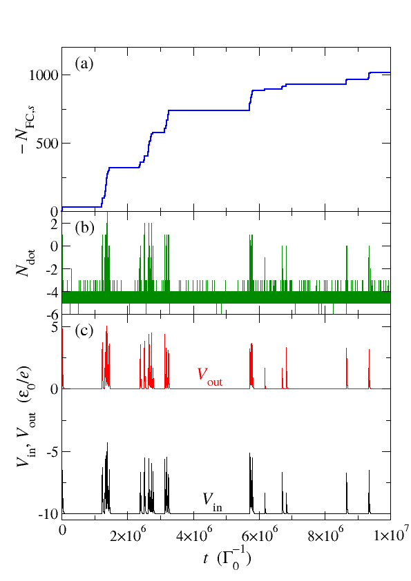
Figure 3: Simulation of the molecular neuron in the ON state for the input current $I_{\mathrm{in}}=-6\times 10^{-4}\,e\Gamma_{0}^{-1}$. The other parameters are given in the text. (a) Change in the number of electrons in the source electrode of the FC molecule, $N_{\mathrm{FC},s}$. (b) Number $N_{\mathrm{dot}}$ of electrons in the quantum dot. (c) Voltages $V_{\mathrm{in}}$ and $V_{\mathrm{out}}$ measured at the input and output contacts of the neuron, respectively.

Results for the ON state are given in figure 3. Here, the input current is $I_{\mathrm{in}}=-6\times 10^{-4}\,e\Gamma_{0}^{-1}$. Figure 3(a) shows the change in the number of electrons in the source electrode of the FC molecule, $N_{\mathrm{FC},s}$. Clearly, the electrons flow in avalanches, typical for the FC regime. Comparison with figure 3 of [8] shows that the auxiliary molecular transistors do not appreciably change this behavior. In particular, feedback from the current through the second auxiliary molecule does not choke off the avalanche-like transport.

In figure 3(b) we plot the number $N_{\mathrm{dot}}$ of electrons in the quantum dot, relative to the neutral state. Negative electron numbers simply mean that the dot is positively charged. The rapid fluctuations are due to electrons tunneling through the barrier between the dot and ground. The electron number preferentially assumes the values $-4$ and $-5$ since these values tune the onsite potential $V_{\mathrm{dot}}$ close to zero, which is the value it would assume in equilibrium with only the ground contact. The avalanches transmitted through the FC molecule are clearly visible. Note that the dot charge stays relatively small so that a large organic molecule or small metallic cluster should be able to accomodate it.

Figure 3(c) shows the input and output voltages, $V_{\mathrm{in}}$ and $V_{\mathrm{out}}$, respectively. $V_{\mathrm{in}}$ contains a constant term resulting from the constant input current. Sharp spikes are evident in both voltages, showing that the active neuron indeed fires voltage spikes into both the input and the output line.

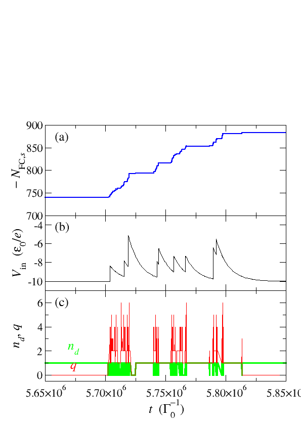
Figure 4: Details of the simulation presented in figure 3 for a shorter time interval. (a) Change in the number of electrons in the source electrode of the FC molecule, $N_{\mathrm{FC},s}$. (b) Voltage $V_{\mathrm{in}}$ measured at the input contact of the neuron. This voltage acts as the gate voltage of the FC molecular transistor. (c) Occupation number $n_{d}$ and harmonic-oscillator quantum number $q$ of the FC molecule.

The spiky voltage $V_{\mathrm{in}}$ is the gate voltage seen by the FC molecular transistor. As we will see below, $V_{\mathrm{in}}$ reaches values that would, if applied continuously, switch off the FC molecule. Nevertheless, the transport through the FC molecule is hardly affected by these spikes, as figure 3 shows. To understand this, we focus on a single series of spikes, taken from the same data as in figure 3. Figures 4(a) and 4(b) show $N_{\mathrm{FC},s}$ and $V_{\mathrm{in}}$, respectively, for a shorter time interval. In figure 4(c) we plot the occupation number $n_{d}$ and the harmonic-oscillator quantum number $q$ of the FC molecule. Evidently, $q\geq 1$ during most of the episode. Thus the FC molecular transistor stores energy in the vibrational mode during the avalanches, which allows it to stay active even though the gate voltage is strongly reduced in magnitude. We see that the memristive properties of the FC molecule are important: The current flowing through it does not only depend on the instantaneous gate and bias voltages but also on its history, here realized by the vibrational quantum number $q$ [33].

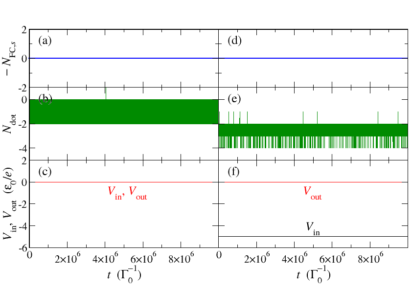
Figure 5: (a)–(c) Simulation of the molecular neuron in the OFF state for vanishing input current, $I_{\mathrm{in}}=0$. The other parameters are the same as for figure 3. (a) Change in the number of electrons in the source electrode of the FC molecule, $N_{\mathrm{FC},s}$. (b) Number $N_{\mathrm{dot}}$ of electrons in the quantum dot. (c) Voltages $V_{\mathrm{in}}$ and $V_{\mathrm{out}}$ measured at the input and output contacts of the neuron, respectively. (d)–(f) The same quantities obtained for the input current $I_{\mathrm{in}}=-3\times 10^{-4}\,e\Gamma_{0}^{-1}$. The other parameters are the same as for figure 3. The neuron is still inactive.

Results for the OFF state are shown in figures 5(a)–(c) for $I_{\mathrm{in}}=0$. The same quantities as for the ON state in figure 3 are plotted. The FC molecule is not transmitting. The quantum dot only shows the fluctuating occupation number due to tunneling through the barrier, which is not sufficient to switch on the auxiliary molecular transistors. We also require the molecular neuron to show threshold behavior—it should not fire spikes for input currents below a certain threshold. Figures 5(d)–(f) show that the device can indeed take a finite input current without becoming active. Here, we have used $I_{\mathrm{in}}=-3\,e\Gamma_{0}^{-1}$, half the value for the active state in figure 3.

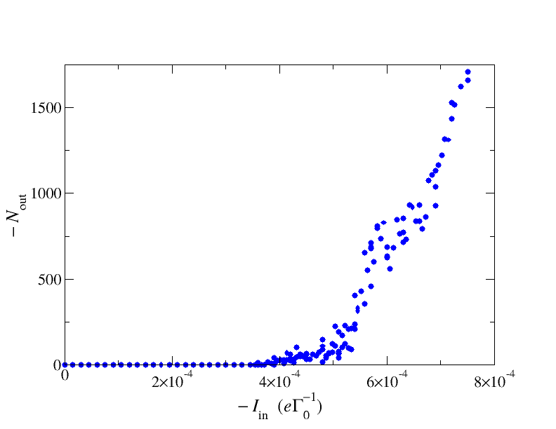
Figure 6: Number $N_{\mathrm{out}}$ of electrons inserted into the drain electrode of the second auxiliary molecule during a simulation time of $t_{\mathrm{sim}}=5\times 10^{7}\,\Gamma_{0}^{-1}$, as a function of the input current $I_{\mathrm{in}}$.

For neural functionality, it is desirable that the switching between OFF and ON states takes place over a narrow range of input currents. To study this onset, we plot in figure 6 the total number $N_{\mathrm{out}}$ of electrons inserted into the drain electrode of the second auxiliary molecule, as a function of the input current $I_{\mathrm{in}}$. A longer simulation time of $t_{\mathrm{sim}}=5\times 10^{7}\,\Gamma_{0}^{-1}$ has been used. There is considerable noise, in particular for intermediate currents, since the FC molecule transmits electrons in avalanches. Between avalanches, the FC molecule returns to the vibrational ground state, $q=0$, and thus does not retain any memory of the previous avalanche. Figure 6 essentially shows the shot noise of independent avalanches. Analysis of the time series (not shown) indicates that the main effect of tuning $I_{\mathrm{in}}$ is to change the delay times between avalanches, not so much their duration. In any case, it is clear that the neuron is inactive over a wide range of input currents.

5 Summary and conclusions

We have proposed a design for a molecular-electronics realization of a neuron. The critical component of this artificial neuron is a molecular transistor with strong electron-vibration coupling, which is tuned to the FC-blockade regime when the neuron is active. In this regime, electrons flow in avalanches. The charge dumped by an avalanche into a small quantum dot or large molecule is used to activate two auxiliary molecular transistors, which lead to voltage pulses traveling along the output line and, importantly, also back up the input line. Employing Monte Carlo simulations for the dynamics of the circuit within the sequential-tunneling approximation, we have demonstrated that the device shows the desired neural behavior. Such a system can be fabricated with experimental capabilities available now or in the near future. It can be used for purposes other than the one discussed here. For instance, with an appropriate choice of system parameters it can operate as an amplifier. Most importantly, it can be used for dynamic storage and transfer of information in complex and highly integrated artificial networks that mimic the behavior of biological neural systems.

References

References

- [1] Russell S J and Norvig P 2009 Artificial Intelligence: A Modern Approach, 3rd edition (Prentice Hall)
- [2] Pershin Y V and Di Ventra M 2011 Phys. Rev. E 84 046703
- [3] Ha S D and Ramanathan S 2011 J. Appl. Phys. 10 071101
- [4] Pershin Y V and Di Ventra M 2010 Neural Networks 23 881
- [5] Le Masson G, Renaud-Le Masson S, Debay D and Bal T 2002 Nature 417 854
- [6] Alibart F, Pleutin S, Guerin D, Novembre C, Lenfant S, Lmimouni K, Gamrat C and Vuillaume D 2010 Adv. Funct. Mat. 20 330
- [7] Di Ventra M and Pershin Y V 2012 Memcomputing: a computing paradigm to store and process information on the same physical platform Preprint arXiv:1211.4487
- [8] Koch J and von Oppen F 2005 Phys. Rev. Lett.94 206804
- [9] Koch J, Raikh M E and von Oppen F 2005 Phys. Rev. Lett.95 056801
- [10] Koch J, von Oppen F and Andreev A V 2006 Phys. Rev. B 74 205438
- [11] Donarini A, Grifoni N and Richter K 2006 Phys. Rev. Lett.97 166801
- [12] Leijnse M and Wegewijs M R 2008 Phys. Rev. B 78 235424
- [13] Hübener H and Brandes T 2009 Phys. Rev. B 80 155437
- [14] Leturcq R, Stampfer C, Inderbitzin K, Durrer L, Hierold C, Mariani E, Schultz M G, von Oppen F and Ensslin K 2009 Nature Phys. 5 317
- [15] Cavaliere F, Mariani E, Leturcq R, Stampfer S and Sassetti M 2010 Phys. Rev. B 81 201303(R)
- [16] Donabidowicz-Kolkowska A and Timm C 2012 New J. Phys.14 103050
- [17] Mitra A, Aleiner I and Millis A J 2004 Phys. Rev. B 69 245302
- [18] Schoeller H and Schön G 1994 Phys. Rev. B 50 18436; König J, Schoeller H and Schön G 1995 Europhys. Lett. 31 31
- [19] Braig S and Flensberg K 2003 Phys. Rev. B 68 205324
- [20] Timm C 2008 Phys. Rev. B 77 195416
- [21] Di Ventra M 2008 Electrical transport in nanoscale systems (Cambridge University Press)
- [22] Stokbro K, Taylor J, Brandbyge M and Guo H 2005 Introducting Molecular Electronics, Lecture Notes in Physics vol 680, edited by Cuniberti G, Fagas G and Richter K (Berlin: Springer Verlag) p 117
- [23] Timm C and Elste F 2006 Phys. Rev. B 73 235304; Elste F and Timm C 2006 Phys. Rev. B 73 235305
- [24] Timm C and Di Ventra M 2012 Phys. Rev. B 86 104427
- [25] Donarini A, Yar A and Grifoni M 2012 Eur. Phys. J. B 85 316
- [26] Schaller G, Krause T, Brandes T and Esposito M 2012 Preprint arXiv:1206.3960
- [27] Park H, Park J, Lim A K L, Anderson E H, Alivisatos A P and McEuen P L 2000 Nature 407 57
- [28] Heersche H B, de Groot Z, Folk J A, van der Zant H S J, Romeike C, Wegewijs M R, Zobbi L, Barreca D, Tondello E and Cornia A 2006 Phys. Rev. Lett.96 206801
- [29] Reed M A, Zhou C, Muller C J, Burgin T P and Tour J M 1997 Science 278 252
- [30] Nakaoka N and Watanabe K 2003 Eur. Phys. J. D 24 397
- [31] Bergfield J P and Stafford C A 2009 Phys. Rev. B 79 245125
- [32] Wu S and Yu J-J 2010 Appl. Phys. Lett. 97 202902
- [33] Pershin Y V and Di Ventra M 2011 Adv. Phys. 60 145