Atomic Quantum Simulation of the Lattice Gauge-Higgs Model: Higgs Couplings and Emergence of Exact Local Gauge Symmetry

Abstract

Recently, the possibility of quantum simulation of dynamical gauge fields was pointed out by using a system of cold atoms trapped on each link in an optical lattice. However, to implement exact local gauge invariance, fine-tuning the interaction parameters among atoms is necessary. In the present Letter, we study the effect of violation of the U(1) local gauge invariance by relaxing the fine-tuning of the parameters and showing that a wide variety of cold atoms is still to be a faithful quantum simulator for a U(1) gauge-Higgs model containing a Higgs field sitting on sites. The clarification of the dynamics of this gauge-Higgs model sheds some light upon various unsolved problems including the inflation process of the early Universe. We study the phase structure of this model by Monte Carlo simulation, and also discuss the atomic characteristics of the Higgs phase in each simulator.

In the past decade, the possibility of using ultracold atoms in an optical lattice (OL) as a simulator for various models in quantum physics seems to have become increasingly more realistic book ; Bloch . In particular, one interesting possibility is to simulate lattice gauge theories (LGTs) by placing several kinds of cold atoms on the links of an OL according to certain rules Buchler ; Tewari ; Weimer ; 1 ; 2 ; 3 ; 4 ; 5 ; 6 ; Wiese . Several proposals for pure U(1) LGTs pure were given in Refs.Buchler ; Tewari ; Weimer ; 1 ; 2 ; 3 and later extended to quantum electrodynamics with dynamical fermionic matter 4 ; 5 and non-Abelian gauge models 6 .

Shortly after their introduction by Wilson wilson , LGTs have been studied quite extensively, mainly in high-energy physics, by using both analytical methods and Monte Carlo (MC) simulations, and their various properties have now been clarified. However, the above-mentioned approach using cold atoms in an OL provides us with another interesting method for studying LGTs. As an example of expected results, the authors of Ref.1 refer to clarification of dynamics of electric strings in the confinement phase. The atomic quantum simulations allow one to address problems which cannot be solved by conventional MC methods because of sign problem. One characteristic point of this cold-atom approach is that the equivalence to the gauge system is established only under some specific conditions. For example, in Refs.1 ; 2 ; 3 ; 4 ; 5 ; 6 , one needs to fine-tune a set of interaction parameters; in other words, the local gauge symmetry is explicitly lost when these parameters deviate from their optimal values.

The above-mentioned point naturally poses us serious and important questions on the stability of gauge symmetry, and potential subtlety of experimental results of cold atoms as simulators of LGTs, because the above conditions are generally not satisfied exactly or easily violated in actual cold-atom systems. In this Letter, we address this problem semi-quantitatively and exhibit the allowed range of violation of the above conditions, such as the regime of interaction parameters, within which the results can be regarded as having LGT properties. In addition, we find that the cold atoms in question may be used as a quantum simulator of a wide class of U(1) gauge-Higgs model, i.e., a Ginzburg-Landau-type model in the London limit coupled with the gauge field, the dynamics of which should offer us important insights on several fields including inflational cosmology inflation .

Let us start with the path-integral representation of the partition function $Z$ of the compact U(1) pure LGT, the reference system of the present study:

$$Z = \int[dU]\exp(A),\ \int[dU]\equiv\prod_{x,\mu}\int_{0}^{2\pi}\frac{d\theta_{x\mu}}{2\pi},$$

$$A = \frac{c_{2}}{2}\sum_{x}\sum_{\mu<\nu}\bar{U}_{x\nu}\bar{U}_{x+\nu,\mu}U_{x+\mu,\nu}U_{x\mu}+{\rm c.c.}$$

$$= c_{2}\sum_{x}\sum_{\mu<\nu}\cos\theta_{x\mu\nu},\ \theta_{x\mu\nu}\equiv\nabla_{\mu}\theta_{x\nu}-\nabla_{\nu}\theta_{x\mu},$$

$$U_{x\mu} \equiv \exp(i\theta_{x\mu}),\ \nabla_{\mu}f_{x}\equiv f_{x+\mu}-f_{x},$$ (1)

where $x=(x_{1},x_{2},x_{3},x_{4})$ is the site index of the 3+1=4D lattice ($x_{4}$ is the imaginary time in the path-integral approach) and $\mu$ and $\nu$ $(=1,2,3,4)$ are the direction indices that we also use as the unit vectors in the $\mu$ and $\nu$-th directions. The angle variable $\theta_{x\mu}\in[0,2\pi)$ and its exponential $U_{x\mu}$ are the gauge variables defined on the link $(x,x+\mu)$ continuum . The bar in $\bar{U}_{x\mu}$ implies complex conjugate, and $c_{2}(\equiv 1/e^{2})$ is the inverse self-gauge-coupling constant. The product of four $U_{x\mu}$ is invariant under the local ($x$-dependent) U(1) gauge transformation,

$$U_{x\mu}\to U^{\prime}_{x\mu}\equiv V_{x+\mu}U_{x\mu}\bar{V}_{x},\ V_{x}\equiv\exp(i\Lambda_{x}),$$ (2)

and so are the field strength $\theta_{x\mu\nu}$ and the action $A$. It is known 4du1 that the system has a weak first-order phase transition at $c_{2}=c_{2c}\simeq 1.0$. For $c_{2}<c_{2c}$ ($>c_{2c}$) the system is in the confinement (Coulomb) phase in which the fluctuations of $\theta_{x\mu}$ are strong (weak). In the Coulomb phase, $\theta_{x\mu}$ describes almost-free massless particles, which correspond to photons in electromagnetism continuum .

To obtain the quantum Hamiltonian $\hat{H}$ for $Z$, let us focus on the space-time plaquette term $\cos\theta_{xi4}$ in $Z$ with the spatial direction index $i(=1,2,3)$ and rewrite it as

$$\exp\left(c_{2}\cos\theta_{xi4}\right)\simeq\sum_{m_{xi}\in{\bf Z}}\exp\left[-\frac{c_{2}}{2}(\theta_{xi4}-2\pi m_{xi})^{2}\right]$$ (3)

$$\propto \sum_{E_{xi}\in{\bf Z}}\exp\left[-iE_{xi}(\nabla_{i}\theta_{x4}-\nabla_{4}\theta_{xi})-\frac{1}{2c_{2}}E_{xi}^{2}\right],$$

where we used the Villain (periodic Gaussian) approximation in the first line and Poisson’s summation formula in the second line. The term $iE_{xi}\nabla_{4}\theta_{xi}\simeq id\tau E_{xi}\dot{\theta}_{xi}$ ($\tau$ is the imaginary time and $\dot{f}\equiv df/d\tau$) shows that the integer-valued field $E_{xi}$ on the spatial link $(x,x+i)$ is the conjugate momentum of $\theta_{xi}$. Thus, the corresponding operators at spatial site $r=(x_{1},x_{2},x_{3})$ satisfy the canonical commutation relation $[\hat{E}_{ri},\hat{\theta}_{r^{\prime}i^{\prime}}]=-i\delta_{rr^{\prime}}\delta_{ii^{\prime}}$. The operator $\hat{E}_{ri}$ represents the electric field in electromagnetism but has integer eigenvalues owing to the compactness (periodicity) of $A$ under $\theta_{x\mu}\to\theta_{x\mu}+2\pi$. The integration over $\theta_{x4}$ can be performed as

$$G \equiv \int\prod_{x}d\theta_{x4}\exp(-i\sum_{x,i}E_{xi}\nabla_{i}\theta_{x4})=\prod_{x}\delta_{Q_{x},0},$$

$$Q_{x} \equiv \sum_{i}\nabla_{i}E_{xi},$$ (4)

where we used $\sum_{x,i}E_{xi}\nabla_{i}\theta_{x4}=-\sum_{x,i}\nabla_{i}E_{xi}\cdot\theta_{x4}$, which holds for a lattice with periodic boundary conditions.

One may check that the quantum Hamiltonian $\hat{H}$ which gives $Z$ at the inverse temperature $\beta$ is just the one given by Kogut and Susskind ks ,

$$\hat{H} = \frac{1}{2c_{2}\Delta\tau}\sum_{r,i}\hat{E}_{ri}^{2}-\frac{c_{2}}{\Delta\tau}\sum_{r,i<j}\cos\hat{\theta}_{rij}$$ (5)

with $\Delta\tau(\equiv\beta/N)$ being the short-time interval in the $\tau$ direction. The $\cos\hat{\theta}_{rij}$ term corresponds to the magnetic energy $(\vec{\nabla}\times\vec{A})^{2}$ in the continuum continuum . In fact, by inserting the complete sets $\hat{1}_{E}=\prod_{r,i}\sum_{E_{ri}}|\{E_{ri}\}\rangle\langle\{E_{ri}\}|$ and $\hat{1}_{\theta}=\prod_{r,i}\int d\theta_{ri}|$$\{\theta_{ri}\}\rangle\langle\{\theta_{ri}\}|$ in between the short-time Boltzmann factors $\exp(-\Delta\tau\hat{H})$, one may derive the relations $Z={\rm Tr}\ \hat{G}\exp(-\beta\hat{H}),\ \hat{G}\equiv\prod_{r}\delta_{\hat{Q}_{r},0}$, and $\hat{Q}_{r}\equiv\sum_{i}\nabla_{i}\hat{E}_{ri}$ constraint . Here, $\hat{Q}_{r}$ is the generator of the time-independent gauge transformation and $\hat{H}$ respects this symmetry as $[\hat{H},\hat{Q}_{r}]=0$. The Gauss’s law $\hat{Q}_{r}=0$ is to be imposed as a constraint for physical states.

Let us discuss the cold-atom studies Buchler ; Tewari ; Weimer ; 1 ; 2 ; 3 ; 4 ; 5 ; 6 ; Wiese , specifically focusing on the quantum simulator using Bose-Einstein condensation (BEC) in an OL 1 . We write the boson operator on the link as $\hat{\psi}_{ri}=\sqrt{\mathstrut\hat{\rho}_{ri}}\exp[(-)^{r}i\hat{\theta}_{ri}],$ $(-)^{r}=(-)^{x_{1}+x_{2}+x_{3}}$, where we use the same letter $\theta_{ri}$ as $\theta_{x\mu}$ in Eq.(1) because the former is to be identified as the latter. We start with the following atomic Hamiltonian 1 ,

$$\hat{H}_{\rm a}\!=\!\sum_{r,a,b}\!\left[g_{ab}\hat{\rho}_{ra}\hat{\rho}_{rb}\!+\frac{V_{0}}{2}\hat{\rho}_{ra}^{2}\!+g^{\prime}_{ab}(\hat{\psi}^{\dagger}_{ra}\hat{\psi}_{rb}+\mbox{H.c.})\right],$$ (6)

where $a,b=1\sim 6$ counts the links emanating from each site. The $g_{ab}$-term describes the densty-density interaction, the $V_{0}(>0)$-term is the on-link repulsion, and the $g^{\prime}_{ab}$-term is the hopping term induced by external electromagnetic fields. We assume that the average $\langle\hat{\rho}_{ri}\rangle=\rho_{0}$ is homogeneous and large, $\rho_{0}\gg 1$, and set $\hat{\rho}_{ri}=\rho_{0}+(-)^{r}\hat{\eta}_{ri}$, where $\hat{\eta}_{ri}$ is the density fluctuation. Then, by choosing $g_{ab}$ and $g^{\prime}_{ab}$ suitably 1 ; 2 ; 3 ; 4 ; 5 ; 6 as $g_{ab}=g\ (>0)$ for any $a$ and $b$, $g^{\prime}_{ab}\simeq 0$ for parallel link pairs, and $g^{\prime}_{ab}=g^{\prime}$ for perpendicular pairs, $\hat{H}_{\rm a}$ is rewritten effectively as

$$\hat{H}_{\rm a} \!= \!\frac{1}{2\gamma^{2}}\sum_{r}\Big{(}\sum_{i}\nabla_{i}\hat{\eta}_{ri}\Big{)}^{2}\!+\!V_{0}\sum_{r,i}\hat{\eta}_{ri}^{2}\!+\hat{H}_{\rm L}(\{\hat{\theta}_{ri}\}),$$

$$\hat{H}_{\rm L} = 2g^{\prime}\rho_{0}\sum_{r,i<j}\left(\cos(\hat{\theta}_{ri}-\hat{\theta}_{rj})+\cdots\right),\$$ (7)

The term with $\gamma^{2}\ (\equiv g^{-1})$ comes from the $g_{ab}$-term and represents the strength of the correlation of fluctuations $\hat{\eta}_{ra}$ around each site (partial conservation of atomic number). We note that setting $g_{ab}$ independent of $a,b$ and controlling its magnitude $g=\gamma^{-2}$ may be achieved by designing the OL suitably or by using interspecies Feshbach resonances 1 ; 2 ; 3 ; 4 ; 5 ; 6 . Some theoretical ideas for the latter are also proposed zpu . $\hat{H}_{\rm L}$ describes the phase correlation between the L-shaped nearest-neighbor (NN) links [the omitted terms in the sum are explicitly written in $A_{\rm L}$ of Eq. (10) below]. We use the coherent state $|\{\psi_{ri}\}\rangle$ and $\hat{1}$$=\prod_{r,i}$$\int d\rho_{ri}$$d\theta_{ri}$ $|\{\psi_{ri}\}\rangle$$\langle\{\psi_{ri}\}|$ to obtain the path-integral for $Z_{\rm a}$$={\rm Tr}$$\ \exp(-\beta\hat{H}_{\rm a})$ as

$$Z_{\rm a} = \!\!\int\prod_{x,i}[d\eta_{xi}d\theta_{xi}]\exp\Big{[}\sum_{x,i}\!\Big{(}\!-i\eta_{xi}\nabla_{4}\theta_{xi}\!-\Delta\tau V_{0}\eta_{xi}^{2}\Big{)}$$ (8)

$$-\frac{\Delta\tau}{2\gamma^{2}}\sum_{x}\Big{(}\sum_{i}\nabla_{i}\eta_{xi}\Big{)}^{2}\!-\!\Delta\tau\sum_{x_{4}}H_{\rm L}(\{\theta_{xi}\})\Big{]}.$$

The first term in the exponent in R.H.S. comes from $\sum_{x_{4}}\bar{\psi}_{xi}\nabla_{4}\psi_{xi}\simeq i\sum_{x_{4}}\eta_{xi}\nabla_{4}{\theta}_{xi}$ and shows that $-\hat{\eta}_{ri}$ is the conjugate momentum of $\hat{\theta}_{ri}$, whereby $\hat{E}_{ri}=-\hat{\eta}_{ri}$.

The Gaussian factor $\tilde{G}\equiv\prod_{x}\exp[(-\Delta\tau/2\gamma^{2})Q_{x}^{2}]$ in Eq. (8) with $Q_{x}\equiv-\sum_{i}\nabla_{i}\eta_{xi}$ shows that the Gauss’s law $Q_{x}=0$ of Eq. (4) is achieved by $\tilde{G}\propto\prod_{x}\delta(Q_{x})$ only at $\gamma\to 0$, and it is now shifted for $\gamma>0$ to a Gaussian distribution with $Q_{x}^{2}\lesssim\gamma^{2}/\Delta\tau$. Thus, $\gamma$ is a parameter used to measure the violation of Gauss’s law. Note that $\tilde{G}$ may be written as

$$\tilde{G}\simeq\!\int_{0}^{2\pi}\!\prod_{x}\!\frac{d\theta_{x4}}{2\pi}\exp\!\left(\!\frac{\gamma^{2}}{\Delta\tau}\cos\theta_{x4}-i\theta_{x4}\sum_{i}\!\nabla_{i}\eta_{xi}\!\right).$$ (9)

By integrating Eq. (8) with Eq. (9) over $\eta_{xi}\in(-\infty,\infty)$, one obtains a term $-(4\Delta\tau V_{0})^{-1}(\nabla_{4}{\theta}_{xi}-\nabla_{i}\theta_{x4})^{2}$, which is a part of Gaussian Maxwell term. However, this result should be improved to respect the periodicity under $\theta_{xi}\to\theta_{xi}+2\pi$, because $\theta_{xi}$ is the phase of the condensate. This Gaussian term is to be replaced, e.g., by a periodic Gaussian form or by the corresponding cosine form $\cos\theta_{xi4}$ as in Eq. (3) (which may be achieved by summing over the integer $\eta_{xi}$). After the summation over $\eta_{xi}$, $Z_{\rm a}$ may be expressed by the following general form;

$$Z_{\rm a} = \int[dU]\exp(A_{\rm a}),\ A_{\rm a}=A_{\rm I}+A_{\rm P}+A_{\rm L},$$

$$A_{\rm I} = \sum_{x,\mu}c_{1\mu}\cos\theta_{x\mu},\ A_{\rm P}=\sum_{x,\mu<\nu}c_{2\mu\nu}\cos\theta_{x\mu\nu},$$

$$A_{\rm L} = \sum_{x,\mu<\nu}c_{3\mu\nu}\Big{[}\cos(\theta_{x\mu}-\theta_{x\nu})+\cos(\theta_{x\mu}+\theta_{x+\mu,\nu})$$ (10)

$$+ \cos(\theta_{x+\mu,\nu}-\theta_{x+\nu,\mu})+\cos(\theta_{x\nu}+\theta_{x+\nu,\mu})\Big{]}.$$

The anisotropic parameters in $A_{\rm a}$ are given as follows; $c_{14}=\gamma^{2}/\Delta\tau,c_{1i}=0$ and $c_{2i4}\simeq(2\Delta\tau V_{0})^{-1}$. $\hat{H}_{\rm L}$ with general values of $g^{\prime}$ directly gives rise to the $A_{\rm L}$ term with $c_{3i4}=0$ and $c_{3ij}=2g^{\prime}\rho_{0}\Delta\tau$, while $c_{2ij}=0$ parallel . We note that, for $g^{\prime}$ much smaller than $\gamma^{-2}$ and/or $V_{0}$, one may treat $\hat{H}_{\rm L}$ as a perturbation. In Refs. 1 ; 2 ; 5 , the case $\gamma\simeq 0$ is considered to enforce the Gauss’s law, and the second-order perturbation theory is invoked to obtain an anisotropic version of the Kogut-Susskind Hamiltonian (5) as an effective Hamiltonian for the gauge-invariant subspace. This implies $c_{2ij}\simeq\gamma^{2}\rho_{0}^{2}{g^{\prime}}^{2}\Delta\tau$ and $c_{3\mu\nu}=0$ in Eq. (10). We refer to this case later as the $\gamma\simeq 0$ case.

Concerning to $c_{1i}$, we note that nonvanishing $c_{1i}$ terms may be incorporated into the cold-atom system by an idea discussed in Ref. c1 ; one may couple to $\hat{\psi}_{ri}$ the atomic field $\hat{a}_{ri}$ in another hyperfine state held in a different trapping potential via the interaction $\hat{H}_{a\psi}=\kappa\sum_{ri}\hat{a}^{\dagger}_{ri}\hat{\psi}_{ri}$+H.c. If $\hat{a}_{ri}$ condenses uniformly at sufficiently high temperatures, $\hat{a}_{ri}$ works as a BEC reservoir and $\hat{H}_{a\psi}$ supplies the $c_{1i}$ term effectively with $c_{1i}=2\kappa|\langle a_{ri}\rangle|\sqrt{\mathstrut{\rho_{0}}}\Delta\tau$. A similar idea is also discussed in Ref. Buchler to generate the $c_{2ij}$ (spatial plaquette) term.

The $A_{\rm I}$ and $A_{\rm L}$ terms in Eq. (10) apparently break U(1) gauge invariance. However, the model $Z_{\rm a}$ of Eq. (10) with general set of parameters is equivalent to another LGT with exact U(1) gauge invariance, i.e., the U(1) gauge-Higgs model containing a Higgs field $\phi_{x}$. $\phi_{x}$ is a complex field defined on site $x$ and takes the form $\phi_{x}=\exp(i\varphi_{x})$, that is its radial excitation is frozen (so-called London limit). The partition function of the U(1) gauge-Higgs model $Z_{\rm GH}(=Z_{\rm a})$ is defined by

$$Z_{\rm GH} = \int[d\phi][dU]\exp A_{\rm GH}(\{U_{x\mu}\},\{\phi_{x}\}),$$

$$A_{\rm GH} = A^{\prime}_{\rm I}+A_{\rm P}+A^{\prime}_{\rm L},\ \int[d\phi]\equiv\prod_{x}\int_{0}^{2\pi}\frac{d\varphi_{x}}{2\pi},$$

$$A^{\prime}_{\rm I} = \sum_{x,\mu}c_{1\mu}\cos(\varphi_{x}+\theta_{x\mu}-\varphi_{x+\mu}),$$

$$A^{\prime}_{\rm L} = \sum_{x,\mu<\nu}c_{3\mu\nu}\Big{[}\cos(\varphi_{x+\nu}+\theta_{x\mu}-\theta_{x\nu}-\varphi_{x+\mu})$$ (11)

$$+\cos(\varphi_{x}+\theta_{x\mu}+\theta_{x+\mu,\nu}-\varphi_{x+\mu+\nu})$$

$$+\cos(\varphi_{x+\mu}+\theta_{x+\mu,\nu}-\theta_{x+\nu,\mu}-\varphi_{x+\nu})$$

$$+\cos(\varphi_{x}+\theta_{x\nu}+\theta_{x+\nu,\mu}-\varphi_{x+\nu+\mu})\Big{]}.$$

$A_{\rm GH}$ in Eq. (11) is gauge invariant under a simultaneous transformation of Eq. (2) and

$$\phi_{x}\equiv e^{i\varphi_{x}}\to\phi^{\prime}_{x}=V_{x}\phi_{x}\hskip 5.69054pt(\varphi_{x} \to \varphi^{\prime}_{x}=\varphi_{x}+\Lambda_{x}).$$ (12)

In fact, $Z_{\rm a}$ is nothing but the gauge-fixed version of $Z_{\rm GH}$ with the so-called unitary gauge $\varphi_{x}=0$. In short, the Higgs field $\phi_{x}$ represents a fictitious charged matter field to describe the violation of chargeless Gauss’s law in ultra-cold atoms, where the general Gauss’s law with a charged field is intact. This relation between a gauge-invariant Higgs model and its gauge-fixed version in the unitary gauge holds for a general action $\tilde{A}(\{U_{x\mu}\})$ as

$$\int[dU]e^{\tilde{A}(\{U_{x\mu}\})}=\int[dU][d\phi]e^{\tilde{A}(\{\bar{\phi}_{x+\mu}U_{x\mu}\phi_{x}\})}.$$ (13)

Eq. (13) is already known in high-energy physics where the standard U(1) gauge-Higgs model is the symmetric one, $c_{1\mu}=c_{1},c_{2\mu\nu}=c_{2},c_{3\mu\nu}=0,$ and used to discuss, e.g., the so-called complementarity relation between excitations in the confinement and Higgs phases complementarity . However, its relevance to the quantum atomic simulator is quite important, because the relation $Z_{\rm a}=Z_{\rm GH}$ leads to a very interesting interpretation that the cold-atom systems proposed in Ref.1 and the other related models 2 ; 3 ; 4 ; 789 with a general set of values of parameters can be used as a simulator of a wider range of field theory, i.e., U(1) LGT including the Higgs couplings. For example, atomic simulations of the standard U(1) gauge-Higgs model above certainly open a new way to understand various phenomena including the inflation process of the early universe inflation and vortex dynamics of bosonized $t$-$J$ model btj .

Let us study the global phase structure of the gauge-Higgs model $Z_{\rm GH}$. We consider the following Models of $Z_{\rm GH}$ for definiteness:

(19)

Model ItPtLs (t denotes time and s denotes space) corresponds to the choice explained below Eq. (10). Model PL with $c_{3}=0$ corresponds to the $\gamma\simeq 0$ case, i.e., the pure gauge theory (5) anisotropy ; smallc2 . Figure 1 shows the phase diagrams of the four Models in Eq.(19) in the $c_{2}$-$c_{1,3}$ plane obtained by standard MC simulations supplement . There are generally three phases—Higgs, Coulomb, and confinement— in the order of increasing size of fluctuations of the gauge field $\theta_{x\mu}$. These three phases can be characterized by the potential energy $V(r)$ stored between two static charges with opposite signs and separated by a distance $r$, as $V(r)\propto 1/r\ ({\rm Coulomb}),\ \exp(-mr)/r\ ({\rm Higgs}),\ r\ ({\rm confinement})$. One may distinguish each phase in the cold atom experiments by measuring atomic density (See Fig.2).

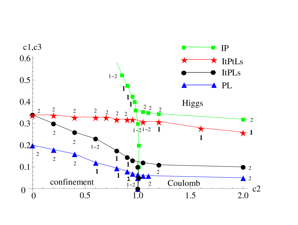
Figure 1: (Color online) Phase diagrams of the four models (19) in the $c_{2}-c_{1,3}$ plane determined by $U=\langle A\rangle$ and $C=\langle A^{2}\rangle-\langle A\rangle^{2}$ calculated by MC simulations for a lattice size of $16^{4}$ supplement . The vertical axis is $c_{1}$ for Model IP, $c_{3}$ for Model PL, and $c_{1}=c_{3}$ for Models ItPtLs and ItPLs. The confinement-Coulomb transition is missing in Model ItPtLs. The number (1, 2) at each critical point indicates its order of transition.The confinement-Higgs line of Model IP terminates at $c_{2}\sim 0.8$.

Figure 1 also shows that the confinement and Coulomb phases of the pure gauge theory along the $c_{2}$ axis survive only up to the phase boundary $c_{1(3)}=c_{1(3)c}(c_{2})$ (except for $c_{2}\lesssim 0.8$ in Model IP); beyond this value of $c_{1(3)}$ the system enters into a new phase, the Higgs phase, in which both $\theta_{x\mu}$ and $\varphi_{x}$ are stable. The expectation that the cold atoms may simulate the pure gauge theory 1 ; 2 ; 5 is assured qualitatively and globally as long as both systems are in the same phase. This occurs for the

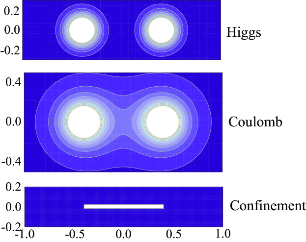
Figure 2: (Color online) Contour plot of the deviation of typical atomic density $\Delta\rho_{r}\equiv(\sum_{i}\eta^{2}_{ri}/3)^{1/2}$ in the $x_{1}-x_{2}$ plane at $x_{3}=0$ with external sources of atoms $\Delta\rho_{\rm ext}=\pm\rho_{1}$ placed on the links emanating from $r=r_{\pm}=(\pm 0.4,0,0)$. The white regions have $\Delta\rho_{r}$ greater than a certain value and the darker regions have lower $\Delta\rho_{r}$ The atomic density on the link $(r,r+i)$ is given by $\rho_{ri}=\rho_{0}+\eta_{ri}$ (here we discard the factor $(-)^{r}$ in front of $\eta_{ri}$ for simplicity), and the deviation $\eta_{xi}$ is calculated by using the electric field $E_{ri}(=-\eta_{ri})$ with a pair of external sources $q=\pm 1$ at $r=r_{\pm}$. In the Higgs phase, $\Delta\rho_{r}$ decreases rapidly away from the sources. In the confinement phase, the deviation propagates from one source to the other along a one-dimensional string (electric flux).

atomic parameters satisfying $c_{1(3)}<c_{1(3)c}(c_{2})$.

The confinement-Coulomb transition exists only for Models having $c_{2i4}\neq 0$ and $c_{2ij}\neq 0$; Model ItPtLs ($c_{2ij}=0$) has no Coulomb phase. This is consistent with the results of pure U(1) gauge theory that the confinement-Coulomb transition exists for 4D system 4du1 but not in the 3D system 2d . For sufficiently large $c_{2i4}$ and $c_{2ij}$, $\theta_{x\mu}$ is almost frozen $\theta_{x\mu}\simeq 0$ up to gauge transformation and the system reduces to the XY model with the XY spin $\phi_{x}=\exp(i\varphi_{x})$. Then, the $c_{1\mu}$ term becomes the NN spin-interaction, $c_{1\mu}\bar{\phi}_{x+\mu}\phi_{x}$, and the $c_{3\mu\nu}$ term becomes the next-NN one, $c_{3\mu\nu}\bar{\phi}_{x+\mu+\nu}\phi_{x}$. These (extended) XY models exhibit a second-order transition both for 3D and 4D couplings, which corresponds to the Higgs-Coulomb transition in Fig. 1. For small $c_{2\mu\nu}$, the confinement-Higgs transition is missing in Model IP ($0\leq c_{2}\lesssim 0.8$), reflecting that $\theta_{x\mu}$ are decoupled at $c_{2}=0$ complementarity . In contrast, in the other three Models, the $c_{3}$ term survives, couples another set of XY spins $\exp(i\theta_{x\mu})$ on NN links, and gives rise to second-order transitions of the XY-model type at $c_{2}\simeq 0$.

It is quite instructive to clarify the physical meaning of the Higgs phase of the gauge system realized in atomic quantum simulators. In the simulator using bosons 1 , the Higgs phase of the effective gauge system is nothing but the BEC state as the phase of the bosons (i.e., the gauge boson) is stabilized coherently. Therefore, the Higgs-confinement transition corresponds to the BEC transition. On the other hand, in Refs. 4 ; 6 , the gauge field is expressed as $\hat{U}_{ri}\simeq(\hat{z}^{\sigma_{r}}_{r+i})^{\dagger}\hat{z}^{\sigma_{r}}_{r}$ ($\sigma_{r}$= 1 for even $r$ and 2 for odd $r$) by using the Schwinger boson $\hat{z}^{\sigma}_{r}$, and the Higgs phase corresponds to the state in which the quantum state at each link $(r,r+i)$ is given by a coherent superposition of the particle-number states such as $|0\rangle_{r}|1\rangle_{r+i}+|1\rangle_{r}|0\rangle_{r+i}$. In the double-well potential, this state is realized naturally, after which the Higgs phase of the gauge system appears easily.

This way of introducing U(1) variables 4 ; 6 reminds us of an approach starting with an antiferromagnet with $s=1/2$ quantum spin at each site and obtaining the CP¹+U(1) LGT sawamura , which has a Schwinger-boson (CP¹) variable at each site describing spins and an auxiliary but dynamical U(1) gauge variables on each link. Although the CP¹+U(1) model and the present U(1) Higgs model are different from each other, their global phase structures are significantly similar (See Fig. 1 of Ref. sawamura ).

In summary, Eq. (11) is the target LGT of cold-atom systems that are basically those studied in Refs. 1 ; 2 but with more general values of interaction parameters and a possible atomic reservoir Buchler ; c1 . Figure 1 predicts its global phase structures. From the discussion given in Refs. 1 ; 2 ; Buchler ; c1 and the relation (13), it may be rather universal that many cold-atom systems with multiplet (“quantum spins”) placed on OL links have their U(1) Higgs LGT counterparts. Such an equivalence between cold atoms and the U(1) gauge-Higgs model may be refereed to as “quantum spin-gauge Higgs correspondence”.

Atomic Quantum Simulation of Lattice Gauge-Higgs Model: Higgs Couplings and emergence of exact gauge symmetry –Supplemental Material–

In this supplemental material, we explain some details to obtain the phase diagram Fig. 1, in particular, how to locate the transition points and determine the order of those transitions. For this purpose, we measure the internal energy $U=\langle A\rangle$ and the specific heat $C=\langle A^{2}\rangle-\langle A\rangle^{2}$ by MC simulations mc . We use the standard Metropolis algorithm metropolis with the periodic boundary condition for the lattice of size $V=L^{4}$ with $L$ up to 24. The typical number of sweeps is $30000+3000*10\sim 100000+10000*10$, where the first number is for thermalization and the second number is for measurement. The errors of $U$ and $C$ are estimated by the standard deviation over 10 samples. Acceptance ratios in updating variables are controlled to be $0.6\sim 0.8$. We check that the hot start ($\theta_{x\mu},\varphi_{x\mu}$ are chosen randomly between $[0,2\pi]$) and the cold start ($\theta_{x\mu}=\varphi_{x\mu}=0$) give the same results within error margin. The results of $U$ and $C$ are checked also by (i) comparison with the high-temperature expansion up to $O(c_{i}^{2})$, which is valid for small $c_{i}$, and (ii) comparison at large $c_{2}$ with independent simulations with setting $U_{x\mu}=1$ which should give similar transition point. In addition, for Model IP in Eq. (14), we make (iii) comparison with the analytic result at $c_{2}=0$ (see Ref. [23] in the text) and (iv) comparison with the result by Jansen et al. jersak in which they study the phase structure of a similar model (Model IP with the radial component of Higgs field $\phi_{x}$ being included).

Figure 3: (Color online) $U/V$ and $C/V$ vs. $c_{1}$ for $c_{2}=2.5$ ($L=16$). $c_{1}$. They indicate a second-order transition at $0.314\lesssim c_{1}\lesssim 0.322$.

Let us pick up some typical transition points for the Model IP in Eq. (14). Every curve of $U$ and $C$ shown below is obtained by first increasing the parameter $c_{1}$ or $c_{2}$ in a fixed interval with an increment $\Delta c_{1(2)}$ and then decreasing it. Such a go-and-back run is useful to detect a hysteresis effect. According to their definitions in thermodynamics, a first-order transition has (i) a gap or a hysteresis loop in $U$ and (ii) a sharp peak in $C$ which usually develops in proportional to the system size $V$, while a second-order transition has (i) a continuous $U$ and (ii) a gap in $C$. In many cases of second-order transitions, $C$ shows a peak which connects lower and higher-valued regions of $C$ and the peak hight develops as the system size is increased 2order .

In Fig. 3 we show $U$ and $C$ vs. $c_{1}$ for $c_{2}=2.5$. The curve $U$ itself as a function of $c_{1}$ is almost continuous except for a small hysteresis loop at $c_{1}\sim 0.315$, but its derivative with respect to $c_{1}$ seems to have a change (almost a gap) at $c_{1}\sim 0.315$. Correspondingly, the curve $C$ globally changes its value from the lower one around $\sim 2.2$ to the higher one around $\sim 4.0$ in the short interval $0.313\lesssim c_{1}\lesssim 0.319$.

These two behaviors accord with the definition of a second-order transition and therefore we conclude that a second-order transition takes place at $0.313\lesssim c_{1}\lesssim 0.319$. Absence of no sharp peak indicates that the associated critical exponent $\sigma$ is small 2order . We judge the hysteresis loop in $U$ is too small as an evidence for a first-order transition.

Figure 4: (Color online) $U/V$ and $C/V$ vs. $c_{1}$ for $c_{2}=0.9$ ($L=16$). A first-order transition takes place at $0.468\lesssim c_{1}\lesssim 0.478$.

Figure 5: (Color online) $U/V$ vs. $c_{1}$ for $c_{2}=0.85$(top) and $c_{2}=0.80$(bottom) ($L=16$). For $c_{2}=0.85$, a weak first-order or a second-order transition takes place at $c_{1}\simeq 0.524$. $U/V$ for $c_{2}=0.80$ shows no jumps nor hysteresis.

In Fig. 4, we show $U$ and $C$ as a function of $c_{1}$ for $c_{2}=0.9$. The clear hysteresis loop indicates the existence of a first-order transition at $0.468\lesssim c_{1}\lesssim 0.478$. The size of corresponding peaks in $C$ seems not large enough as a first-order transition, but such a phenomenon often takes place and is attributed to the finiteness of $\Delta c_{1}$.

In Fig. 5, we show $U$ as a function of $c_{1}$ for $c_{2}=0.85$ (top) and $c_{2}=0.80$ (bottom). For $c_{2}=0.85$, $U$ exhibits a step-function-like behavior at $c_{1}\simeq 0.524$, although no hysteresis loop appears with the present increment $\Delta c_{1}=0.002$. We judge that a weak first-order or a second-order transition takes place there. On the other hand, for $c_{2}=0.8$, $U$ looks smooth showing no gap and hysteresis loop. Therefore we judge that no first-order transition takes place. Concerning to the possibility of a second-order transition, we check whether the peak of $C$ at $c_{1}\simeq 0.58$ develops as the system size $L$ is increased 2order . Our preliminary analysis using $L=20,24$ shows that the size-dependence is rather weak, although the errors in $C$ are too large to draw a definitive conclusion. For a lower value $c_{2}=0.75$, $U$ and $C$ is smoother, and in particular, $C$ spreads wider than $c_{2}=0.80$. From these observation, we conclude that the line of transition should terminate at $0.75\lesssim c_{2}\lesssim 0.85$.

Figure 6: (Color online) $U/V$ and $C/V$ vs. $c_{2}$ for $c_{1}=0.3$($L=16$). There is a weak first-order or a second-order transition at $c_{2}\simeq 1.01$.

In Fig. 6 we show $U$ and $C$ vs. $c_{2}$ for $c_{1}=0.3$. $U$ has two branches that meet at $c_{2}\sim 1.01$ with different slopes and a small hysteresis loop. We conclude that there is a weak first-order or a second-order transition at $c_{2}\simeq 1.01$.

It is certainly true that more number of sweeps and smaller increments, $\Delta c_{i}$, certainly give rise to smaller errors in $U$ and $C$ and more precise determination of the location and the order of the transition points. However, the allowed size of errors in the location of the transition points drawn in Fig. 1 in the text is about $\Delta c_{i}\simeq 0.02$, i.e., almost same as the size of the marks drawn there, and therefore the accuracy of the present MC study is almost sufficient for the purpose to draw Fig. 1 in the text. On the other hand, definitive determination of the order of phase transition for some points requires more detailed study by the MC simulations. We hope to report on this subject in a future publication.

References

(1)
M. Lewenstein, A. Sanpera, and V. Ahufinger, Ultracold Atoms in Optical Lattices:
Simulating Quantum Many-body Systems (Oxford University Press, 2012).
(2)
I. Bloch, J. Dalibard, and S. Nascimbene,
Nat. Phys. 8, 267 (2012).
(3)
H. P. Büchler, M. Hermele, S. D. Huber, M. P. A. Fisher, and P. Zoller,
Phys. Rev. Lett. 95, 040402 (2005).
(4)
S. Tewari, V. W. Scarola, T. Senthil, and S. Das Sarma,
Phys. Rev. Lett. 97, 200401 (2006).
(5)
H. Weimer, M. Muller, I. Lesanovsky, P. Zoller, and H. P. Büchler,
Nat. Phys. 6, 382 (2010).
(6)
E. Zohar and B. Reznik,
Phys. Rev. Lett. 107, 275301 (2011).
(7)
E. Zohar, J. I. Cirac, and B. Reznik,
Phys. Rev. Lett. 109, 125302 (2012).
(8)
L. Tagliacozzo, A. Celi, A. Zamora, and M. Lewenstein,
Ann. Phys. 330, 160 (2013).
(9)
D. Banerjee, M. Dalmonte, M. Müller, E. Rico, P. Stebler, U.-J. Wiese,
and P. Zoller, Phys. Rev. Lett. 109, 175302 (2012).
(10)
E. Zohar, J. I. Cirac, and B. Reznik,
Phys. Rev. Lett. 110, 055302 (2013).
(11)
E. Zohar, J. I. Cirac, and B. Reznik, Phys. Rev. Lett. 110, 125304 (2013);
D. Banerjee, M.Bögli, M. Dalmonte, E. Rico, P. Stebler, U.-J. Wiese,
and P. Zoller, Phys. Rev. Lett. 110, 125303 (2013);
L. Tagliacozzo, A. Celi, P. Orland, and M. Lewenstein, arXiv:1211.2704.
(12)
U. -J. Wiese, arXiv:1305.1602 (2013).
(13)
The word “pure” implies that the system
contains only gauge fields and no other
fields such as quarks, etc.
We use it for the system with below
in Eq. (10).
(14)
K. Wilson, Phys. Rev. D 10, 2445 (1974);
J. B. Kogut, Rev. Mod. Phys. 51, 659 (1979).
(15)
A. H. Guth, Phys. Rev. D 23, 347 (1981);
E. Kolb and M. Turner, “The Early Universe”, Westview Press, (1994);
A. D. Linde, Lect. Notes Phys. 738, 1 (2008).
(16)
is related to the vector potential in the continuum
space-time as where is the lattice
spacing. In the formal continuum limit ,
the action is reduced to
with
as it should be. The partition function can be defined without a gauge fixing
due to the compactness in contrast with .
(17)
See, e.g., E. Sa’nchez-Velasco, Phys. Rev. E 54, 5819 (1996),
and references cited therein.
(18)
J. Kogut and L. Susskind, Phys. Rev. D 11, 395 (1975).
(19)
To respect in ,
one needs to insert at least only once
at any in the path-integral due to .
In other words, one may insert it at every
as done in Eq.(4) due to the equalities,
.
(20)
P. Zhang, P. Naidon, and M. Ueda. Phys. Rev. Lett. 103, 133202 (2009).
(21)
Inclusion of the parallel hopping terms to of Eq. (6)
such as
(both and ) is straightforward
and brings the corresponding Higgs couplings in Eqs. (10) and (11).
(22)
A. Recati, P. O. Fedichev, W. Zwerger, J. von Delft, and P. Zoller,
Phys. Rev. Lett. 94, 040404 (2005).
(23)
E. Fradkin and S. H. Shenker,
Phys. Rev. D 19, 3682 (1979).
(24)
Strictly speaking, Refs. 2 ; 3 ; 4 deal with the subspace
(the so-called U(1) gauge magnet) instead of .
For a large , which corresponds to (),
the two models may have similar behaviors,
because Eq. (5) with
restricts to effectively.
Quantitative comparison of these two models in a general setting
is an interesting problem.
(25)
See, e.g., K. Aoki, K. Sakakibara, I. Ichinose and T. Matsui,
Phys. Rev. B 80, 144510 (2009).
(26)
The anisotropic pure gauge theory is expected to have
the similar global phase structure as the symmetric one
as long as all are nonvanishing.
See the review by J. B. Kogut in Ref. wilson .
(27)
We note in the case of Refs. 1 ; 2 cannot become
arbitrarily large due to its perturbative origin.
(28)
Some technical details of the MC simulations for Model IP in Eq. (19)
are described in the supplemental material.
(29)
The 3D version of the pure U(1) gauge theory (1)
is always in the confinement phase (no Coulomb phase) [A. M. Polyakov, Phys. Lett. B 59, 82 (1975)].
For cold atoms in the 2D OL 1 ; 2 , the target LGT
is the 2+1=3D U(1) LGT with NN and/or next-NN Higgs couplings.
The 3D Model IP lives only in the confinement phase, while
the 3D couplings of in the other 3D Models
may generate confinement-Higgs transitions.
(30)
K. Sawamura, T. Hiramatsu, K. Ozaki, I. Ichinose, and T. Matsui,
Phys. Rev. B 77, 224404 (2008).

References

(1)
For more details on the present method to determine a phase structure by
MC simulations, see, e.g., Refs. [25,30] cited in the text.
(2)
N. Metropolis, A. W. Rosenbluth, M. N. Rosenbluth, A. M. Teller,
E. Teller, J. Chem. Phys. 21, 1087 (1953).
(3)
K. Jansen, J. Jersák, C. B. Lang, T. Neuhaus, G. Vones,
Nucl. Phys. B 265, 129 (1986).
(4)
According to the finite-size scaling hypothesis
[See, e.g., L. P. Kadanoff, Physics 2, 263 (1966)],
near the second-order transition point behaves for large as
for large ,
where and
is the critical point for .
is the scaling function, and are
the critical exponents.