Proposals which speed-up function-space MCMC

Abstract

Inverse problems lend themselves naturally to a Bayesian formulation, in which the quantity of interest is a posterior distribution of state and/or parameters given some uncertain observations. For the common case in which the forward operator is smoothing, then the inverse problem is ill-posed. Well-posedness is imposed via regularisation in the form of a prior, which is often Gaussian. Under quite general conditions, it can be shown that the posterior is absolutely continuous with respect to the prior and it may be well-defined on function space in terms of its density with respect to the prior. In this case, by constructing a proposal for which the prior is invariant, one can define Metropolis-Hastings schemes for MCMC which are well-defined on function space ([1, 2]), and hence do not degenerate as the dimension of the underlying quantity of interest increases to infinity, e.g. under mesh refinement when approximating PDE in finite-dimensions. However, in practice, despite the attractive theoretical properties of the currently available schemes, they may still suffer from long correlation times, particularly if the data is very informative about some of the unknown parameters. In fact, in this case it may be the directions of the posterior which coincide with the (already known) prior which decorrelate the slowest. The information incorporated into the posterior through the data is often contained within some finite-dimensional subspace, in an appropriate basis, perhaps even one defined by eigenfunctions of the prior. We aim to exploit this fact and improve the mixing time of function-space MCMC by careful rescaling of the proposal. To this end, we introduce two new basic methods of increasing complexity, involving (i) characteristic function truncation of high frequencies and (ii) Hessian information to interpolate between low and high frequencies. The second, more sophisticated version, bears some similarities with recent methods which exploit local curvature information, for example RMHMC [3], and stochastic Newton [4]. These ideas are illustrated with numerical experiments on the Bayesian inversion of the heat equation and Navier-Stokes equation, given noisy observations.

1 Introduction

Sampling distributions over high-dimensional state-spaces is a notoriously difficult problem, and a lot of effort has been devoted to developing methods to do this effectively [5, 6, 7, 2]. If a given target distribution is known pointwise, then Markov chain Monte Carlo is a general method which prescribes a Markov chain having this target distribution as its invariant distribution. Examples include Metropolis-Hastings schemes, developed first by [8] and later generalized for arbitrary proposals by [9]. It is well known that Metropolis-Hastings schemes developed for finite-dimensional systems degenerate in the limit of inference on infinite-dimensional spaces and a lot of work has been devoted to examining the actual rate with which they degenerate [6]. Indeed this analysis has led to improved performance of chains in finite dimensions through arguments about optimal scaling of the acceptance probability. Recently, it has been shown in a series of works by [5, 2, 1] that it is possible to overcome this limitation by defining the Metropolis-Hastings scheme in function space, thus confronting the issue of high dimensions head on. This is particularly useful, for example, in the case where the system is a finite-dimensional approximation of a PDE. In such a case, the convergence properties of the function-space scheme are independent of mesh refinement which increases the dimension of the finite-dimensional approximating system. However, it may (and often does in practice) happen that, even though the scheme is defined on function-space and is hence independent of mesh refinement, the integrated autocorrelation may be quite large for certain degrees of freedom, in particular those which have small effect on the likelihood. Hence, there is clearly a paradox in that the degrees of freedom which are not informed by the data, and hence are governed by the prior, are the rate limiting factor in the convergence of MCMC. But, at the same time, more is known a priori about such degrees of freedom. We aim to maintain the positive aspect of being defined in function space while removing the deficit of mixing poorly in directions which are better known a priori. This will be accomplished by appropriate rescaling based on curvature which leverages a priori known information. Inspired by the works [5, 2, 1] we will focus on sampling distributions $\mu$ over some Hilbert space $H$ which have density with respect to a Gaussian reference measure $\mu_{0}$ of the following form

$$\mu(du)=Z\exp[-\Phi(u)]\mu_{0}(du),$$ (1.1)

where $\Phi:H\rightarrow\mathbb{R}$, and $Z=1/\int_{H}\exp[-\Phi(u)]\mu_{0}(du)$. For simplicity, we let

$$\Phi(u)=\frac{1}{2\gamma^{2}}|G(u)-y|^{2},$$ (1.2)

and we will further assume that $G(u)$ is a compact operator. This function arises as the negative log likelihood of $u\sim\mu_{0}$ given a realization of an observation $y=G(u)+\eta$, where $\eta\sim\mathcal{N}(0,\gamma^{2}I)$ independent of $u$. The posterior distribution on $u$, conditioned on the particular observation $y$, is given by (1.1). Furthermore, we will assume that $\mu_{0}=N(m,C)$ for some trace-class operator $C$.

The rest of this paper will be organized as follows. In Section 2, we will provide a review of necessary concepts, including the recently developed function-space MCMC method pCN [2] which will serve as a starting point for this work. In Section 3 we illustrate the remaining decorrelation issues pertaining to proposal chains of the pCN form. In Section 4 we introduce a class of constant operator rescaled proposals which address the issues highlighted in Section 3 and yet still fit into the function-space sampler framework, hence taking full advantage of its benefits. In Section 5, we investigate the performance of these algorithms computationally against standard pCN for the inverse heat equation and inversion of Navier-Stokes equation. Finally, we provide conclusions and possible future directions in Section 6.

2 Background

In this section we give some background on Markov chain Monte Carlo (MCMC) methods, and in particular the Metropolis-Hastings (MH) variants. We then introduce the preconditioned Crank-Nicolson (pCN) proposal that yields an MH algorithm which is well-defined on function spaces for a wide range of posterior distributions of the form (1.1), for example those arising from the Bayesian interpretation of the solution to an inverse problem with Gaussian prior and observational noise. Finally, we will describe the way that correlations enter into approximations based on the resulting set of samples and define the effective sample size, which will be relevant in the derivation of the new methods which follow.

2.1 MCMC

MCMC methods aim to sample from a target distribution $\mu$ over $H$ by designing a Markov transition kernel $\mathcal{P}$ such that $\mu$ is invariant under the action of $\mathcal{P}$

$$\int_{H}\mu(du)\mathcal{P}(u,dv)=\mu(dv),$$ (2.1)

with shorthand ($\mu\mathcal{P}=\mu$), where the integral on the lefthand side is with respect to $du$. The condition known as detailed balance between a transition kernel $\mathcal{P}$ and a probability distribution $\mu$ says that

$$\mu(du)\mathcal{P}(u,dv)=\mu(dv)\mathcal{P}(v,du),\quad\forall~{}u,v\in H.$$ (2.2)

Integrating with respect to $u$, one can see that detailed balance implies $\mu\mathcal{P}=\mu$. Metropolis-Hastings methods prescribe an accept-reject move based on proposals from an arbitrary transition kernel $\mathcal{Q}$ in order to define a kernel $\mathcal{P}$ such that detailed balance with an arbitrary probability distribution is guaranteed. In order to make sense of MH in infinite dimensions, first define the measures [10]

$$\begin{array}[]{lll}\nu(du,dv)&=&\mathcal{Q}(u,dv)\mu(du)\\ \nu^{T}(du,dv)&=&\mathcal{Q}(v,du)\mu(dv).\end{array}$$ (2.5)

Provided $\nu^{T}\ll\nu$, where $\ll$ is denoting absolutely continuity when comparing measures, one can define the MH kernel as follows. Given current state $u_{n}$, a proposal is drawn $u^{*}\sim\mathcal{Q}(u_{n},\cdot)$, and then accepted with probability

$$\alpha(u_{n},u^{*})={\rm min}\left\{1,\frac{d\nu^{T}}{d\nu}(u_{n},u^{*})\right\}.$$ (2.6)

The resulting chain has transition kernel $\mathcal{P}$ given by

$$\mathcal{P}(u,dv)=\alpha(u,v)\mathcal{Q}(u,dv)+\delta_{u}(dv)\int_{X}(1-\alpha(u,w))\mathcal{Q}(u,dw).$$ (2.7)

So, we have that

$$\mu(du)\mathcal{P}(u,dv)={\rm min}\left\{\mathcal{Q}(u,dv)\mu(du),\mathcal{Q}(v,du)\mu(dv)\right\}+$$

$${\rm max}\left\{0,\delta_{u}(dv)\left[\mu(du)-\int_{X}\mathcal{Q}(w,du)\mu(dw)\right]\right\}$$ (2.8)

which one can see satisfies the necessary symmetry condition (2.2) . Under an additional assumption of geometric ergodicity, one has that $|\mathcal{P}^{n}(u_{0},\cdot)-\mu|_{\rm TV}\rightarrow 0$ for any $u_{0}\in H$ [11]. Therefore, after a sufficiently long equilibration period, or burn-in, one has a prescription for generating samples approximately distributed according to $\mu$, from which integrals with respect to $\mu$ can be approximated. These samples are correlated, however, and this will be revisited below.

Since there is great freedom in choice of proposal kernel $\mathcal{Q}$, one can imagine that there is great discrepancy in the performance of the algorithms resulting from different choices. It is popular to choose symmetric kernels, such as the classical random walk algorithm, in which the difference between the current and proposed states is taken to be a centered Gaussian distribution, e.g.

$$\mathcal{Q}(u_{n},\cdot)=\mathcal{N}(u_{n},\beta^{2}C),$$

where $C$ is the covariance of the prior $\mu_{0}$. For this proposal, the absolute continuity condition $\nu^{T}\ll\nu$ is violated, so the MH algorithm is defined only in finite dimensions [1] and degenerates under mesh refinement. However, a small modification to the classical random walk proposal

$$\mathcal{Q}(u_{n},\cdot)=\mathcal{N}(\sqrt{1-\beta^{2}}(u_{n}-m)+m,\beta^{2}C)$$ (2.9)

yields an algorithm which satisfies $\nu^{T}\ll\nu$ since $\mathcal{Q}$ and $\mu_{0}$ are in detailed balance. This algorithm is therefore defined on function space, and it is referred to as pCN in [2]. The key point here is that the posterior has a density with respect to the infinite-dimensional prior Gaussian measure $\mu_{0}$ and so designing a proposal such as the one above which is reversible with respect to this measure leads to the necessary condition $\nu^{T}\ll\nu$. The condition that $\nu^{T}\ll\nu$ for algorithms on function space ensures that the methods are well-behaved with respect to mesh refinement; only such methods are considered in this paper (see [2] for more details on that point). The choice of proposal $\mathcal{Q}$ which satisfies detailed balance with the prior $\mu_{0}$ is natural and elegant because it leads to acceptance probability $\alpha(u,v)$ which depends only on the ratio of the likelihood evaluated at its arguments

$$\alpha(u,v)={\rm min}\left\{1,e^{\Phi(u)-\Phi(v)}\right\}.$$ (2.10)

2.2 Correlations

Let $R:H\rightarrow\mathbb{R}$, and suppose we would like to estimate the integral $\mathbb{E}(R)=\int_{H}R(u)\mu(du)$ by $N$ samples $R_{n}=f(u_{n})$, where $u_{n}\sim\mu$. Denoting this estimate by $\bar{R}$, we have

$$\bar{R}=\frac{1}{N}\sum_{n=1}^{N}R_{n}.$$

Then $\mathbb{E}(\bar{R})=\mathbb{E}(R)$, so the estimator is without bias. Furthermore, we denote the variance of $R$ by

$$\mathbb{V}(R)=\mathbb{E}[(R-\mathbb{E}(R))(R-\mathbb{E}(R))].$$

So, we also have that

$$\mathbb{V}(\bar{R})=\mathbb{E}[(\bar{R}-\mathbb{E}(R))(\bar{R}-\mathbb{E}(R))].$$

We restrict attention to the case $\mathbb{E}(R)=0$, for ease of exposition only. Assume also that the samples are correlated in such a way that

$$\rho_{n}=\mathbb{E}(R_{m}R_{m+n})/\mathbb{E}(R_{m}R_{m})~{}~{}\forall m,n.$$

For example, such samples arise from a sample path of a homogeneous Markov chain, such as in MCMC. Then

$$\begin{array}[]{lll}\mathbb{V}(\bar{R})&=&\mathbb{E}[\bar{R}\bar{R}]\\ &=&(1/N^{2})\left(\sum_{n=1}^{N}R_{n}R_{n}+\sum_{n,m=1,n\neq m}^{N}R_{n}R_{m}\right)\\ &\approx&(1/N)\mathbb{V}(R)(1+2\sum_{n=1}^{N}\rho_{n})\\ &=&\frac{(1+2\theta)}{N}\mathbb{V}(R),\end{array}$$ (2.15)

where we assumed $\rho_{n}\approx 0$ for all $n>N^{*}$ with $N^{*}\ll N$, and we denoted $\theta=\sum_{n=1}^{N}\rho_{n}$. If the $R_{n}$ are independent then $\theta=0$ and we recover constant prefactor $1$ to $\mathbb{V}(R)/N$. Otherwise, the constant prefactor reduces the effective number of samples with respect to the case of independent samples. It is therefore informative to define the effective sample size by $N_{eff}=N/(1+2\theta)$. Phrased another way, one needs $1+2\theta$ samples in order to get another approximately independent sample. Hence, $\rho_{n}$ and $\theta$ are referred to as the autocorrelation function and the integrated autocorrelation, respectively. The general case is dealt with similarly, working elementwise. In this case, the effective sample size is given by the minimum over effective sample sizes of individual degrees of freedom, strictly speaking.

From the above discussion, it is clear that the performance of an MH algorithm in approximating integrals with respect to a distribution is limited by the correlation between the samples it generates. The rest of the paper will concern this point about correlations.

3 Proposal Chains for MCMC

In this section, we explore some drawbacks of the function-space sampling algorithm defined in the previous section. We will first motivate the need for modification with a simple one dimensional example. Then, we describe how this same idea lifts into higher dimensions.

3.1 Principle in 1d

Figure 1: Illustration of slow decorrelation in proposal chain $X$, and fast decorrelation in the informed chain $Z$. Left plot shows autocorrelations, as compared also to the analytical autocorrelation of $X$. Right plot shows an interval of the evolution over which $X$ has barely decorrelated, but $Z$ has clearly decorrelated within a small sub-interval.

As an example, consider the following Markov chain

$$X_{n+1}=(1-\beta^{2})^{1/2}X_{n}+\beta W_{n}$$

where $X_{0},W_{n}\sim\mathcal{N}(0,\sigma^{2})$ i.i.d. for all $n$ and $\beta<1$. So, $\mathbb{E}X_{n}=0$ for all $n$, and

$$X_{n}=(1-\beta^{2})^{n/2}X_{0}+\beta\sum_{k=0}^{n-1}(1-\beta^{2})^{(n-1-k)/2}W_{k}.$$

Therefore, $\rho_{n}=\mathbb{E}(X_{0}X_{n})/\mathbb{E}(X_{0}X_{0})=(1-\beta^{2})^{n/2}\approx\exp(-n\beta^{2}/2)$, and $\theta=\sum_{n=1}^{N}\rho_{n}\approx 2/\beta^{2}.$ Notice also that this is independent of $\sigma$.

Now, we run an experiment. Let $\phi(z)=(1/2\gamma^{2})(z-1)^{2}$, with $\gamma=0.01$ and $\sigma=1$. Consider the following Metropolis-Hastings chain $Z$ with proposal given by $X$:

$$\begin{array}[]{c}Z^{*}=(1-\beta^{2})^{1/2}Z_{n}+\beta W_{n}\\ Z_{n+1}\sim\alpha\delta(Z^{*}-~{}\cdot)+(1-\alpha)\delta(Z_{n}-~{}\cdot),\quad\alpha=1\wedge\exp(\phi(Z_{n})-\phi(Z^{*})).\end{array}$$ (3.1)

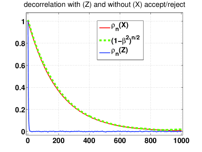
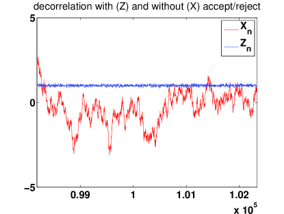
The above chain samples the posterior distribution with observation $y=z+\mathcal{N}(0,\gamma^{2})=1$ and prior $Z\sim\mathcal{N}(0,1)$. We will denote the chains by $X=\{X_{n}\}$ and $Z=\{Z_{n}\}$ Figure 1 illustrates the decorrelation time and evolution of the proposal chain, $X$, and the informed chain $Z$ for a given choice of $\beta$ which yields reasonable acceptance probability. The speedup is astonishing, and indeed counterintuitive: one only accepts or rejects moves from the proposal chain, so intuition may suggest that the informed chain would have larger autocorrelation. But actually, if the distribution is dominated by the likelihood, then the integrated autocorrelation is determined by the accept/reject, and is indeed smaller than that of the proposal. On the other hand, if the distribution is dominated by the prior, then the integrated autocorrelation is dictated by the proposal chain and is then increased by the acceptance probability. If the state-space were two dimensional, with an observation only in the first dimension, then for a given choice of scalar $\beta$ the chain will mix like $Z$ in the observed component and like $X$ in the unobserved component. The same idea extends to higher dimensions, motivating the use of direction-dependent proposal step-sizes.

Figure 2: Expected acceptance probability (top) and lag 1 autocorrelation (bottom) over $\beta$ with $\gamma=0.01$ (left) and over $\gamma$ with $\beta=0.05$ fixed (right), for proposals which are reversible with respect to the prior (blue) and the posterior (red dashed). Also shown at the bottom is the lag 1 autocorrelation of the proposal chain, $\sqrt{1-\beta^{2}}$, in black dash-dotted.

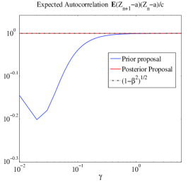
We now digress momentarily to explain this counterintuitive phenomenon in more detail for the simple analytically solvable example above. This is crucial to understanding the methods which will be developed in subsequent sections. In the above example, the posterior distribution is given by $\mathcal{N}(a,c)$, where $a=1/(\gamma^{2}+1)$ and $c=\gamma^{2}/(1+\gamma^{2})$. Assuming that $Z_{n}\sim\mathcal{N}(a,c)$, we know from Eqs. 3.1 that the correlation between subsequent steps is given by the following analytically known, yet horrendous, integral

$$\begin{array}[]{lll}\frac{1}{c}\mathbb{E}[(Z_{n+1}-a)(Z_{n}-a)]&=&\frac{1}{2\pi c\sqrt{c}}\int_{\mathbb{R}^{2}}[z^{*}-a)(z-a)\alpha(z,z^{*})+\\ &&(z-a)^{2}(1-\alpha(z,z^{*}))]e^{-[\frac{(z-a)^{2}}{2c}+\frac{1}{2}w^{2}]}dzdw,\end{array}$$ (3.2)

where $z^{*}=\sqrt{1-\beta^{2}}z+\beta w$. It is instructive to also consider in Eq. (3.1) the alternative proposal which keeps the posterior invariant:

$$Z^{*}=(1-\beta^{2})^{1/2}(Z_{n}-a)+a+\sqrt{c}\beta W_{n},$$ (3.3)

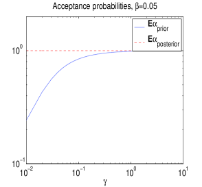
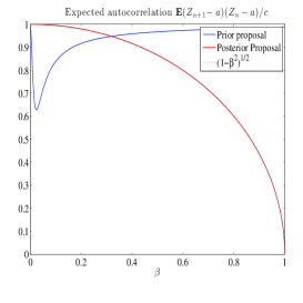
in which case $z^{*}=\sqrt{1-\beta^{2}}(z-a)+a+\sqrt{c}\beta w$ in Eq. (3.2) and the acceptance (2.10) is modified accordingly. Indeed, it turns out that $\frac{1}{c}\mathbb{E}[(Z_{n+1}-a)(Z_{n}-a)]\leq\sqrt{1-\beta^{2}}$, with equality in the limit of $\mathbb{E}\alpha\rightarrow 1$. See also [6]. We compute this integral using a Riemann sum and plot the corresponding values of $\alpha$ and $\frac{1}{c}\mathbb{E}[(Z_{n+1}-a)(Z_{n}-a)]$ for varying $\beta$ with $\gamma$ fixed, and varying $\gamma$ with $\beta$ fixed in Fig. 2. In the top left panel, we see that for proposal (3.1) with $\gamma=0.01$ the acceptance decreases from 1 to 0 as $\beta$ ranges from 0 to 1. In the bottom left panel below this we can see that the minimum lag 1 autocorrelation corresponds to the acceptance probability $\mathbb{E}\alpha\approx 0.5$; c.f. the well-known optimal scaling results of [6]. For the proposal (3.3), the acceptance is 1 for all $\beta$. It is clear from the bottom left plot that in this example we should use (3.3) with $\beta=1$ and do independence sampling on the known posterior. This obvious result in this idealistic example is instructive, however. It is not possible to do independence sampling on the posterior for non-Gaussian posteriors (or we would be done) and even independence sampling on the Gaussian approximation to the posterior may lead to unacceptably small acceptance probability. Indeed we can see that the prior proposal can perform as well as or better than the posterior proposal for appropriate $\beta<0.75$, a step-size that is probably much too large in a Gaussian proposal whenever the target is non-Gaussian. This makes it clear that the crucial thing is to choose the appropriate scale of the proposal steps, rather than naively trying to match the target with the proposal (although this principle does hold for the case presented above in which the proposal keeps the target posterior invariant, and in general this does lead to reasonably effective proposals). From the top right panel, we can see that the acceptance probability for the posterior proposal is again 1 for all $\gamma$ for a fixed $\beta=0.05$, while the autocorrelation (bottom right) also remains approximately $\sqrt{1-\beta^{2}}$ (which is quite large in this case). However, as this choice of $\beta$ is tuned to the prior proposal for $\gamma=0.01$, we see that the acceptance probability for prior proposal increases from $0.25$ to almost 1 as $\gamma$ ranges from $0.01$ to 5. The corresponding lag 1 autocorrelation ranges from $0.63$ to approximately $\sqrt{1-\beta^{2}}$ as $\gamma$ increases and the posterior approaches the prior.

3.2 Higher dimensions

Recall that in one dimension if the distribution is determined by the likelihood then the integrated autocorrelation is close to 1, and if the distribution is determined by the prior then the integrated autocorrelation is dictated by the proposal chain. Suppose that some of the space is dominated by the prior, and some is dominated by the likelihood. If the observations have small variance, then the step-size $\beta$ in the chain will have to be small in order to accommodate a reasonable acceptance probability. But, the part of the space which is dominated by the prior will have $O(1/\beta^{2})$ autocorrelation, as dictated by the proposal chain.

Now consider the Bayesian inverse problem on a Hilbert space $H$. Let $\{\varphi_{j}\}_{j=1}^{\infty}$ denote an orthonormal basis for the space $H$. Let $P$ project onto a finite basis $\{\varphi_{j}\}_{j=1}^{J}$ and $Q=I-P$. Suppose we wish to sample from the posterior distribution $\mu$ with prior distribution $\mu_{0}$, where $d(\mu(Q\cdot),\mu_{0}(Q\cdot))\ll\epsilon$ for some $\epsilon\ll 1$ and some distance function $d(\cdot,\cdot)$ between probability measures (for example Hellinger metric or Kullback-Leibler distance). Thus $P$ projects onto the “important part” of the space, in the sense that the observations only inform the projection of the posterior distribution on this part of the space. Suppose we use Metropolis-Hastings to sample from posterior $\mu$ with prior $\mu_{0}=\mathcal{N}(0,C)$. Let $u_{0},W_{n}\sim\mathcal{N}(0,C)$, so that the pCN chain

$$u_{n+1}=(1-\beta^{2})^{1/2}u_{n}+\beta W_{n}$$ (3.4)

leaves the prior invariant. Without loss of generality, we represent this chain in the basis in which $C$ is diagonal, so the proposal for each degree of freedom is an independent version of the above and clearly has decorrelation time $1+2\theta\approx 4/\beta^{2}$. The distribution $\mu\approx\mu_{0}$ on $QH$, so when we impose accept/reject using the above chain as proposal, we are sampling from $\mu(Q\cdot)$ with decorrelation time $(1+2\theta)/\mathbb{E}\alpha$ where $\mathbb{E}\alpha$ is the expected acceptance probability. But, we may as well sample independently from the known distribution $\mu_{0}(Q\cdot)$ in this part of the space.

Following the reasoning above, one can consider modifying the above proposal chain to sample from the pCN chain (3.4) on $PH$ and sample independently from the prior on $QH$. This corresponds to setting the chain above to

$$u_{n+1}=(1-\beta^{2})^{1/2}Pu_{n}+(\beta P+Q)W_{n}.$$ (3.5)

Our first and simplest variant of weighted proposal follows directly from this. In the next section we will consider a more elaborate extension of this proposal using curvature information.

4 Operator weighted proposal

Inspired by the discussion in the preceding section, we let $B_{n}$ be an operator weighting different directions differently, and define the proposal chain to be

$$u_{n+1}=\sqrt{B_{n}}u_{n}+\sqrt{I-B_{n}}W_{n}.$$ (4.1)

with $u_{0},W_{n}\sim\mathcal{N}(0,I)$. Notice that this proposal preserves the prior in the sense that $u_{n}\sim\mathcal{N}(0,I)~{}~{}\forall n$. This form of proposal for $B_{n}=B$ constant in $n$ can be derived as a generalization of the pCN proposal from [2], for some general pre-conditioner $\mathcal{K}$ in their notation.

Recall the form of distribution we consider, given by (1.1) and (1.2), with prior of the form $u\sim\mathcal{N}(m,C)$. For simplicity of exposition, we will consider standard normal $\mathcal{N}(0,I)$ priors, without any loss of generality. In the general case, a change of variables $u\rightarrow C^{1/2}u+m$ is imposed to normalize the prior, such that a chain of the form (4.1) keeps the prior invariant. The samples of the resulting MH chain are then transformed back as $u\rightarrow C^{-1/2}(u-m)$ for inference.

For the moment, we revert to the case in which $H=\mathbb{R}^{N}$ in order to motivate the form of the proposals. In this case we have $\mu\ll\lambda$, where $\lambda$ is Lebesgue measure, and after transformation

$$-{\rm log}\left[\frac{d\mu}{d\lambda}(u)\right]=\Phi(u)+\frac{1}{2}|u|^{2}+K(y),$$ (4.2)

with $K(y)=\int_{H}\exp\{-[\Phi(u)+\frac{1}{2}|u|^{2}]\}d\lambda$. At a given point $w$ the local curvature is given by the Hessian of this functional, which can be approximated by the positive definite operator

$$\frac{1}{\gamma^{2}}DG(w)^{*}DG(w)+I,$$ (4.3)

where $DG(w)$ denotes the derivative of $G$ with respect to $u$ evaluated at $w$ . If $\{\lambda_{k},\phi_{k}\}$ are eigenpairs associated with this operator, then:

• if $\lambda_{k}\gg 1$, then the distribution is dominated by the data likelihood in the direction $\phi_{k}$;

• if $\lambda_{k}\approx 1$, then the distribution is dominated by the prior in the direction $\phi_{k}$.

The direction of the largest curvature at a given point will determine the smallest scale of the probability distribution at that point. If $\lambda_{1}$ is the largest eigenvalue of (4.3), then the smallest local scale of the density will be $\sqrt{1/\lambda_{1}}$. This scale will directly determine the step-size necessary to obtain a reasonable acceptance probability within the MH algorithm. But, such a small step-size is only necessary in the direction $\phi_{1}$. So, rather than prescribing this as the step-size in the remaining directions, we would like to rescale them according to the operator given in (4.3).

There is no log-density with respect to Lebesgue measure in function space, but the above operator (4.3) is still well-defined and indeed its minimizer gives the point of maximum probability over small sets [15]. This functional will be the basis for choosing $B_{n}$ in (4.1). Based on the above intuition, one can devise a whole hierarchy of effective such operators. In the simplest instance, one can allow for $B_{n}$ constant, either during the duration of the algorithm, after a transient adaptive phase, or even for some lag-time where it is only updated every so often. In this manuscript we consider only constant $B$, and we consider three simple levels of complexity. The rigorous theory underlying the algorithms will be deferred to future work, although we note that the case of constant $B$ is easier to handle theoretically, since one does not need to consider the conditions for ergodicity of adaptive MCMC [12].

The first level of complexity consists of letting

$$B=(1-\beta^{2})I.$$ (4.4)

The resulting method corresponds to the original pCN proposal, and we denote this method by O.

The second level of complexity consists of letting

$$B_{k,j}=(1-\beta^{2}){\bf 1}_{k<k_{c}}\delta_{k,j},$$ (4.5)

where $B=\{B_{k,j}\}_{k,j=1^{\infty}}$, $\delta_{k,j}$ is the Kronecker delta function, and $k_{c}\in(0,k_{\rm max}]$ and $\beta\in(0,1]$ are chosen during a transient adaptive phase, either together or one at a time, yielding (3.5). The simple idea is that the curvature is constant and prescribed by the prior for sufficiently high frequencies, and this has already been motivated by the discussion in the previous section. The method resulting from this proposal will be denoted by C.

The third level of complexity consists of utilizing a relaxed version of the Hessian for an arbitrary given point close to a mode of the distribution. Let

$$B = (1-\beta^{2})(DG(w)^{*}DG(w)+\zeta\gamma^{2}I)^{-1}DG(w)^{*}DG(w),$$ (4.6)

where $\beta$ is the scalar tuning parameter as in the above cases, $\zeta\in(0,1]$ is another tuning parameter, and $w$ is any point. The method resulting from this proposal will be denoted by H. We consider a low rank approximation of the resulting operator, since it is assumed to be compact. Notice that for this choice of $B$, the covariance of the search direction is given by

$$I-B = (DG(w)^{*}DG(w)/(\zeta\gamma^{2})+I)^{-1}+$$ (4.7)

$$\beta^{2}(DG(w)^{*}DG(w)+\zeta\gamma^{2}I)^{-1}DG(w)^{*}DG(w).$$

For linear $G$ we let $\zeta=1$, and the right-hand side of the above approaches the covariance of the posterior distribution as $\beta\rightarrow 0$, giving exactly the correct rescaling for the search direction while still keeping the prior invariant. The linear case is rather special, since we could just do independence sampling of the posterior, but it provides a good benchmark. In practice, adaptation of $\beta$ in this case leads to small, but non-zero, $\beta$. For nonlinear $G$ we choose $\zeta<1$, and the scaling of the search direction is commensurate with the local curvature except with increased weight on the log-likelihood component, given by the first term of (4.7). The second term is a perturbation which is larger for the (changing) directions dictated by the Hessian of the log-likelihood and approaches zero for directions which are dictated by the prior, in which the curvature is constant. Provided $\zeta$ is chosen small enough, and the curvature does not change too much, the step-size of a given move will not exceed the scale of the distribution. Furthermore, the step-size will interpolate appropriately between the direction of the smallest scale and the directions which are determined by the prior, corresponding to scale 1. We note that a whole array of different proposals are possible by choosing different $B_{n}$, and there may be better options since an exhaustive search has not been carried out. Investigation into various other proposals which incorporate the appropriate (re)scaling in different ways, however, suggests that their performance is similar [16].

Both methods C and H can be considered as splitting methods in which part of the space is targeted using the acceptance probability and independence sampling is done on the complement. C splits the spectral space into a finite inner radius in which pCN is done, and its infinite-dimensional complement where independence sampling is done. H more delicately splits the space into the finite dominant eigenspace of the Hessian of the likelihood $DG^{*}(w)DG(w)$ and its complement, and then furthermore considers an appropriate rescaling of the dominant eigenspace. Notice that the complement space absorbs the infinite-dimensionality. Such proposals which separate the space allow any general form of proposal on the finite-dimensional target subspace and maintain the property that $\nu^{T}\ll\nu$ as long as the proposal is reversible with respect to the prior on the infinite-dimensional complement subspace. For example, a simple pCN proposal with another choice of $\beta$ can be used on this subspace. This idea appears in the forthcoming works [16, 17].

Note that one could instead incorporate this curvature information by devising a chain which keeps a Gaussian approximation to the posterior invariant, similarly to (3.3). For example, one can use the following proposal which preserves $\mathcal{N}(\xi,\Xi)$:

$$u_{n+1}=\Xi^{1/2}\sqrt{1-B_{n}}\Xi^{-1/2}(u_{n}-\xi)+\xi+(\Xi B_{n})^{1/2}W_{n},$$ (4.8)

with $u_{0}\sim\mathcal{N}(\xi,\Xi)$ and $W_{n}\sim\mathcal{N}(0,I)$. The curvature information can be incorporated for example by letting

$$\xi={\rm argmin}_{u}\left[\Phi(u)+\frac{1}{2}|u|^{2}\right],$$

or some close by point, and $\Xi=(\frac{1}{\gamma^{2}}DG(\xi)^{*}DG(\xi)+I)^{-1}$. In this case, it would be sensible to revert to the case of scalar $B_{n}$ since the relevant scaling is already intrinsic in the form of the Gaussian. Empirical statistics can also be incorporated in this way. If $DG(\xi)^{*}DG(\xi)$ is genuinely low-rank then equivalence $\nu^{T}\ll\nu$ is immediate. If not, one must look more closely. However, in this case if one imposes a low-rank approximation, then equivalence is again immediate based on the discussion above. The results in Sec. 3.1, and in particular those presented in Fig. 2 illustrate that this strategy should not be considered as preferable to using a proposal of the form (4.1) for appropriate choice of $B_{n}$. These variations do however warrant further investigation. We limit the current study to the case of proposals of the form (4.1) because (i) these methods are defined on function space, following immediately from the reversibility with respect to the prior and the framework of [10], (ii) the acceptance probability takes the simple and elegant form of (2.10) which is easy to implement, and (iii) as described in Sec. 3, it is not clear that a more elaborate kernel such as the one following from the proposal (4.8) would yield better results.

5 Numerical Results

In this section, we will investigate the performance of the MH methods introduced in the previous section on two prototypical examples. First, we briefly explore the inverse heat equation on the circle as an illustrative example. Next, we look in more depth at the more complicated problem of the inverse Navier-Stokes equation on the 2D torus.

5.1 Heat Equation

Consider the one dimensional heat equation

$$\frac{\partial v}{\partial t}-\frac{\partial^{2}v}{\partial x^{2}} = 0$$

$$v(t,0)=v(t,\pi) = 0.$$

We are interested in the inverse problem of recovering $u=v(0,x)$ from noisy observations of $v(1,x)$:

$$y = v(1,x)+\eta$$

$$= Gu+\eta,$$

where $G=\exp\{-A\}$, $A=(-\frac{d^{2}}{dx^{2}})$, $D(A)=H^{2}(\Omega)\cap H^{1}_{0}(\Omega)$ with $\Omega=(0,\pi)$, and $\eta\sim N(0,\gamma^{2}I).$ We let $C=10^{4}A^{-1}$, and $\gamma=1$.

The problem may be solved explicitly in the Fourier sine basis, and the coefficients of the mean $m_{k}$ and variance $V_{k}$ of the posterior distribution can be represented in terms of the coefficients of the data $y_{k}$ and the prior $C_{k,k}=10^{4}k^{-2}$:

$$m_{k} = (e^{-2k^{2}}+10^{4}k^{2})^{-1}e^{-k^{2}}y_{k},$$

$$V_{k} = (e^{-2k^{2}}+10^{4}k^{2})^{-1}.$$ (5.1)

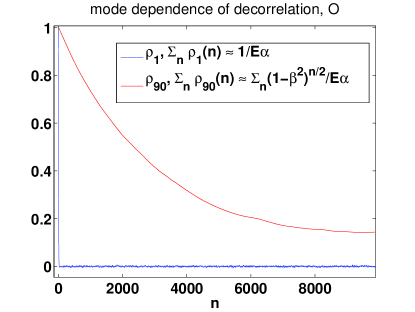
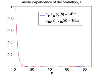
The posterior distribution is strongly concentrated on the $u_{1}$ mode, in the sense that $m_{1}\gg m_{j}$ and $V_{1}\gg V_{j}$ for all $j>1$, and the discrepancy between $\Gamma$ and $C$ will necessitate a very small scalar $\beta$. For the case of scalar weighting O, all modes will decorrelate slowly except for $u_{1}$. See Fig. 3 for a comparison between scalar weighting O and curvature-based weighting H. In this case, we will omit the intermediate proposal which simply proposes independent samples outside a certain radius in the spectral domain.

Figure 3: Illustration of the autocorrelation of modes $u_{1}$ and $u_{90}$, in the case of O (left), and H (right).

5.2 Navier-Stokes Equation

In this section, we consider the inverse problem of determining the initial condition of Navier-Stokes equation on the two dimensional torus given noisy observations. This problem is relevant to data assimilation applications in oceanography and meteorology.

Consider the 2D Navier-Stokes equation on the torus $\mathbb{T}^{2}:=[-1,1)\times[-1,1)$ with periodic boundary conditions:

$$\begin{array}[]{cccc}\partial_{t}v-\nu\Delta v+v\cdot\nabla v+\nabla p&=&f&{\rm for~{}all~{}}(x,t)\in\mathbb{T}^{2}\times(0,\infty),\\ \nabla\cdot v&=&0&{\rm for~{}all~{}}(x,t)\in\mathbb{T}^{2}\times(0,\infty),\\ v&=&u&{\rm for~{}all~{}}(x,t)\in\mathbb{T}^{2}\times\{0\}.\end{array}$$

Here $v\colon\mathbb{T}^{2}\times(0,\infty)\to\mathbb{R}^{2}$ is a time-dependent vector field representing the velocity, $p\colon\mathbb{T}^{2}\times(0,\infty)\to\mathbb{R}$ is a time-dependent scalar field representing the pressure, $f\colon\mathbb{T}^{2}\to\mathbb{R}^{2}$ is a vector field representing the forcing (which we assume to be time independent for simplicity), and $\nu$ is the viscosity. We are interested in the inverse problem of determining the initial velocity field $u$ from pointwise measurements of the velocity field at later times. This is a model for the situation in weather forecasting where observations of the atmosphere are used to improve the initial condition used for forecasting. For simplicity we assume that the initial velocity field is divergence free and integrates to zero over $\mathbb{T}^{2}$, noting that this property will be preserved in time.

Define

$${\mathcal{H}}:=\left\{{\rm{\,trigonometric\,polynomials\,}}u\colon\mathbb{T}^{2}\to{\mathbb{R}}^{2}\,\Bigl{|}\,\nabla\cdot u=0,\,\int_{\mathbb{T}^{2}}u(x)\,\mathrm{d}x=0\right\}$$

and $H$ as the closure of ${\mathcal{H}}$ with respect to the $(L^{2}(\mathbb{T}^{2}))^{2}$ norm. We define $P\colon(L^{2}(\mathbb{T}^{2}))^{2}\to H$ to be the Leray-Helmholtz orthogonal projector (see [13]). Given $k=(k_{1},k_{2})^{\mathrm{T}}$, define $k^{\perp}:=(k_{2},-k_{1})^{\mathrm{T}}$. Then an orthonormal basis for $H$ is given by $\psi_{k}\colon\mathbb{R}^{2}\to\mathbb{R}^{2}$, where

$$\psi_{k}(x):=\frac{k^{\perp}}{|k|}\exp\Bigl{(}\pi ik\cdot x\Bigr{)}$$

for $k\in\mathbb{Z}^{2}\setminus\{0\}$. Thus for $u\in H$ we may write

$$u=\sum_{k\in\mathbb{Z}^{2}\setminus\{0\}}u_{k}(t)\psi_{k}(x)$$

where, since $u$ is a real-valued function, we have the reality constraint $u_{-k}=-\bar{u}_{k}$. Using the Fourier decomposition of $u$, we define the fractional Sobolev spaces

$$H^{s}:=\Bigl{\{}u\in H\Bigm{|}\sum_{k\in\mathbb{Z}^{2}\setminus\{0\}}(\pi^{2}|k|^{2})^{s}|u_{k}|^{2}<\infty\Bigr{\}}$$ (5.3)

with the norm $\|u\|_{s}:=\bigl{(}\sum_{k}(\pi^{2}|k|^{2})^{s}|u_{k}|^{2}\bigr{)}^{1/2}$, where $s\in\mathbb{R}$. If $A=-P\Delta$, the Stokes’ operator, then $H^{s}=D(A^{s/2})$. We assume that $f\in H^{s}$ for some $s>0$.

Let $t_{n}=nh$, for $n=0,\dots,N$, and let $v_{n}\in\mathbb{R}^{M}$ be the set of pointwise values of the velocity field given by $\{v(x_{m},t_{n})\}_{m=1}^{M/2}$. Note that each $v_{n}$ depends on $u$ and define $G_{n}\colon H\to\mathbb{R}^{M}$ by $G_{n}(u)=v_{n}$. We let $\{{\eta}_{n}\}_{n=1}^{N}$ be a set of random variables in $\mathbb{R}^{M}$ which perturbs the points $\{v_{n}\}_{n=1}^{N}$ to generate the observations $\{y_{n}\}_{n=1}^{N}$ in $\mathbb{R}^{M}$ given by

$$y_{n}:=v_{n}+\gamma{\eta}_{n},\quad n\in\{1,\ldots,N\}.$$ (5.4)

We let $y=\{y_{n}\}_{n=1}^{N}$ denote the accumulated data up to time $T=Nh$, with similar notation for $\eta$, and define $G\colon H\to\mathbb{R}^{MN}$ by $G(u)=\bigl{(}G_{1}(u),\dots,G_{N}(u)\bigr{)}$. We now solve the inverse problem of finding $u$ from $y=G(u)+\eta$. We assume that the prior distribution on $u$ is a Gaussian $\mu_{0}=N(0,C_{0})$, with the property that $\mu_{0}(H)=1$ and that the observational noise $\{\eta_{n}\}_{n=1}^{N}$ is i.i.d. in $\mathbb{R}^{M}$, independent of $u$, with $\eta_{1}$ distributed according to a Gaussian measure $N(0,\gamma^{2}I)$.

We let $C_{0}=\pi^{4}A^{-2}$ noting that if $u\sim\mu_{0}$, then $u\in H^{s}$ almost surely for all $s<1$; in particular $u\in H$. Thus $\mu_{0}(H)=1$ as required. The forcing in $f$ is taken to be $f=\nabla^{\perp}\Psi$, where $\Psi=(2/\pi)(\cos(\pi k_{c}\cdot x)+\sin(\pi k_{s}\cdot x)$ and $\nabla^{\perp}=J\nabla$ with $J$ the canonical skew-symmetric matrix, $k_{c}=(5,5)$ and $k_{s}=(-5,5)$. Furthermore, we let the viscosity $\nu=0.1$, and the interval between observations $h=\delta t=0.05$, where $\delta t$ is the timestep of the numerical scheme, and $N=10$ so that the total time interval is $T=Nh=0.5$. In this regime, the nonlinearity is mild and the attractor is a fixed point, similar to the linear case. Nonetheless, the dynamics are sufficiently nonlinear that the optimal proposal used in the previous section does not work. We take $M=32^{2}$ evaluated at the gridpoints, such that the observations include all numerically resolved, and hence observable, wavenumbers in the system. The observational noise standard deviation is taken to be $\gamma=3.2$.

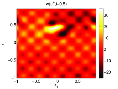
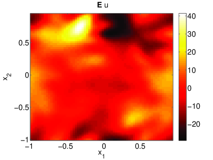
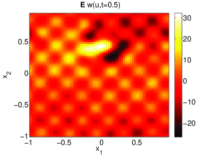
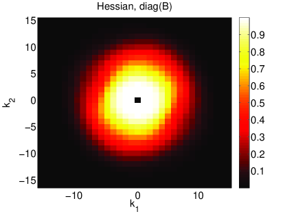
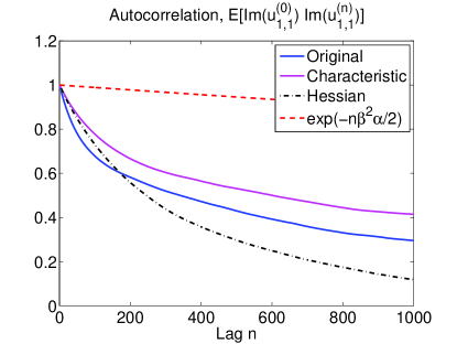
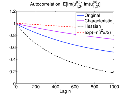
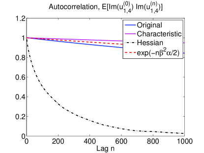
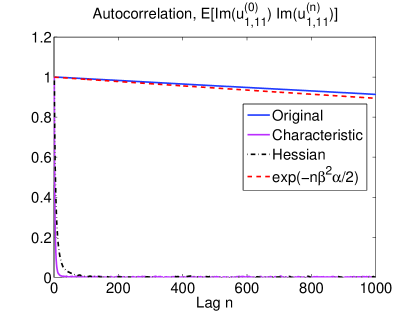
The truth and the mean vorticity initial conditions and solutions at the end of the observation window are given in Fig. 4. The truth (top panels) clearly resembles a draw from a distribution with mean given by the bottom panels. Fig. 5 shows the diagonal of the rescaling operator $B$ (i.e. for $\beta=0$) for C, given by (4.4) and H, given by (4.5). For O the operator is given by the identity, i.e. all one along the diagonal. Some autocorrelation functions (approximated with one chain of $10^{6}$ each) are shown in Fig. 6. Also given for comparison is the exponential fit to the (acceptance lagged) autocorrelation function for the proposal chain for O, i.e. $\exp(-n\beta^{2}\mathbb{E}\alpha/2)$. This differs for each, because $\beta$ and $\mathbb{E}\alpha$ differ. In particular, for O $\beta=0.024$ and $\mathbb{E}\alpha\approx 0.41$ (approximated by the sample mean), for C $\beta=0.015$ and $\mathbb{E}\alpha\approx 0.32$, and for H $\beta=0.015$ and $\mathbb{E}\alpha\approx 0.25$. Presumably this accounts for the slight discrepancy in the autocorrelation of mode $u_{1,1}$, given in the top left panel. For the mode $u_{1,2}$ (top right), the difference becomes more pronounced between H and the other two. In the bottom left it is clear that the mode $u_{1,4}$ decorrelates very quickly for H, while it decorrelates approximately like the proposal chain for both other methods. The mode $u_{1,11}$ (bottom right) is independently sampled for C, so has decorrelation time $1/\mathbb{E}\alpha$. It decorrelates almost as fast for H, and is decorrelating with the proposal chain for O.

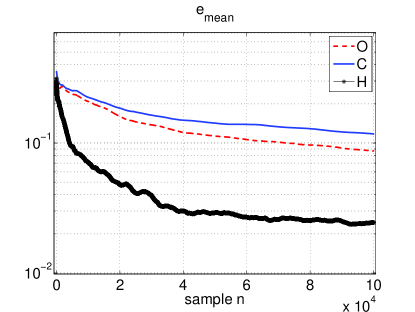
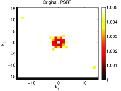
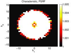
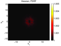
Figure 7 shows the relative error in the mean (left) and variance (right) with respect to the converged values as a function of sample number for small sample sizes. The accumulated benefit of H is very apparent here, yielding almost an order of magnitude improvement. For each of the proposals, we run $16$ chains of length $10^{6}$, both for the benchmark mean and variance used in Fig. 7, and to compare the so-called potential scale reduction factor (PSRF) convergence diagnostic [14]. In Fig. 8 we plot the PSRF for each method on the same color scale from $[1,1.005]$. Although it cannot be seen for O(left) and C(middle) since the values of most modes are saturated on this scale, every mode for every method is clearly converged according to the PSRF, which should be smaller than 1.1 and eventually converges to 1. We can see for O that the low frequencies, where the mean and uncertainty are concentrated, converge faster (as indicated in 6), and other modes converge more or less uniformly slowly. C clearly outperforms O in the high frequencies outside the truncation radius (where the mean and uncertainty are negligible) and is comparable for the smallest frequencies, but may even be worse than O for the intermediate frequencies. This may be explained by the different $\beta$ and $\mathbb{E}\alpha$. Again, H quite clearly outperforms both of the other two methods. Note that these results are for particular parameter choices, and methods of choosing the parameters $\beta$, $k_{c}$, $\zeta$, and may be sensitive to their choice.

Figure 4: Truth (top) and expected value of the posterior (bottom). Initial condition is given to the left and solution at final time is given to the right.

Figure 5: The diagonal of the rescaling operator $B$ for C, given by (4.5) and H, given by (4.6).

Figure 6: The autocorrelation for each method O, C, and H, for a variety of frequencies. Also given for comparison is the exponential fit to the (acceptance lagged) autocorrelation function for the proposal chain for O, i.e. $\exp(-n\beta^{2}\mathbb{E}\alpha/2)$. This differs for each, because $\beta$ and $\mathbb{E}\alpha$ differ.

Figure 7: The relative error in the mean (left) and variance (right) with respect to the converged values as a function of sample number for small sample sizes.

Figure 8: The PSRF plots for O (left), C (middle) and H (right). The images are saturated on the same scale so that H is visible.

6 Conclusions

This manuscript introduces and investigates a new class of proposals for function-space MCMC, giving rise to a new class of algorithms. These proposals involve an operator which appropriately rescales the proposal step-sizes in different directions in order to decrease autocorrelation and hence improve convergence rate. For the curvature-inspired rescaling H introduced here, there are two design parameters which need to be hand-chosen. But, it seems to be effective to choose $\zeta$ sufficiently small and then allow $\beta$ to be chosen during a transient adaptive phase, as in the other methods. It should be possible to achieve the same result with one design parameter. Furthermore, there exists a whole range of more sophisticated models between those investigated here and the more sophisticated but expensive RMHMC [3] and stochastic Newton [4]. This gives rise to exciting opportunities for future investigation. It will be of great interest to establish rigorous theoretical results, such as geometric ergodicity, for these methods.

Acknowledgements The author would like to thank EPSRC and ONR for financial support. I also thank The Mathematics Institute and Centre for Scientific Computing at Warwick University, as well as The Institute for Computational and Experimental Research in Mathematics and The Center for Computation and Visualization at Brown University for supplying valuable computation time. I would like to extend thanks to Tiangang Cui, Youssef Marzouk, and Gareth Roberts for interesting discussions related to these results, and also to the referee for a careful read and insightful suggestions for improvement. Finally, I thank Andrew Stuart for interesting discussions related to these results and for valuable input in the revision of this manuscript.

References

- [1] A. Stuart, Inverse problems: a Bayesian approach, Acta Numer. 19 (2010) 451–559.
- [2] S. Cotter, G. Roberts, A. Stuart, D. White, MCMC methods for functions: modifying old algorithms to make them faster, Arxiv preprint arXiv:1202.0709.
- [3] M. Girolami, B. Calderhead, Riemann manifold Langevin and Hamiltonian Monte Carlo methods, Journal of the Royal Statistical Society: Series B (Statistical Methodology) 73 (2) (2011) 123–214.
- [4] J. Martin, L. Wilcox, C. Burstedde, O. Ghattas, A stochastic newton mcmc method for large-scale statistical inverse problems with application to seismic inversion, SIAM Journal on Scientific Computing 34 (3) (2012) 1460–1487.
- [5] A. Beskos, G. O. Roberts, A. M. Stuart, J. Voss, MCMC methods for diffusion bridges, Stochastic Dynamics 8 (3) (2008) 319–350. doi:10.1142/S0219493708002378.
- [6] G. Roberts, A. Gelman, W. Gilks, Weak convergence and optimal scaling of random walk Metropolis algorithms, Ann. Appl. Prob. 7 (1997) 110–120.
- [7] G. Roberts, R. Tweedie, Exponential convergence of Langevin distributions and their discrete approximations, Bernoulli 2 (4) (1996) 341–363.
- [8] N. Metropolis, R. Rosenbluth, M. Teller, E. Teller, Equations of state calculations by fast computing machines, J. Chem. Phys. 21 (1953) 1087–1092.
- [9] W. Hastings, Monte carlo sampling methods using markov chains and their applications, Biometrika 57 (1970) 97–109.
- [10] L. Tierney, A note on Metropolis-Hastings kernels for general state spaces, Ann. Appl. Probab. 8 (1) (1998) 1–9.
- [11] M. Hairer, A. Stuart, S. Vollmer, Spectral gaps for a Metropolis-Hastings algorithm in infinite dimensions, Arxiv preprint arXiv:1112.1392.
- [12] G. Roberts, J. Rosenthal, Coupling and ergodicity of adaptive markov chain monte carlo algorithms, Journal of applied probability 44 (2) (2007) 458–475.
- [13] J. C. Robinson, Infinite-Dimensional Dynamical Systems, Cambridge Texts in Applied Mathematics, Cambridge University Press, Cambridge, 2001.
- [14] S. Brooks, A. Gelman, General methods for monitoring convergence of iterative simulations, Journal of Computational and Graphical Statistics 7 (4) (1998) 434–455.
- [15] M. Dashti, K.J.H. Law, A.M. Stuart and J. Voss, MAP estimators and posterior consistency in Bayesian nonparametric inverse problems. Accepted for publication in Inverse Problems (2013). http://arxiv.org/abs/1303.4795 .
- [16] T. Cui, K.J.H. Law, and Y. Marzouk, Likelihood-informed sampling of Bayesian nonparametric inverse problems. In preparation (2013).
- [17] A. Beskos, A. Jasra, N. Kantas, (Submitted, 2013). http://arxiv.org/abs/1307.6127 .